


Forest Structure Mapping of Boreal Coniferous Forests Using Multi-Source Remote Sensing Data

Abstract

1. Introduction
2. Study Area and Data
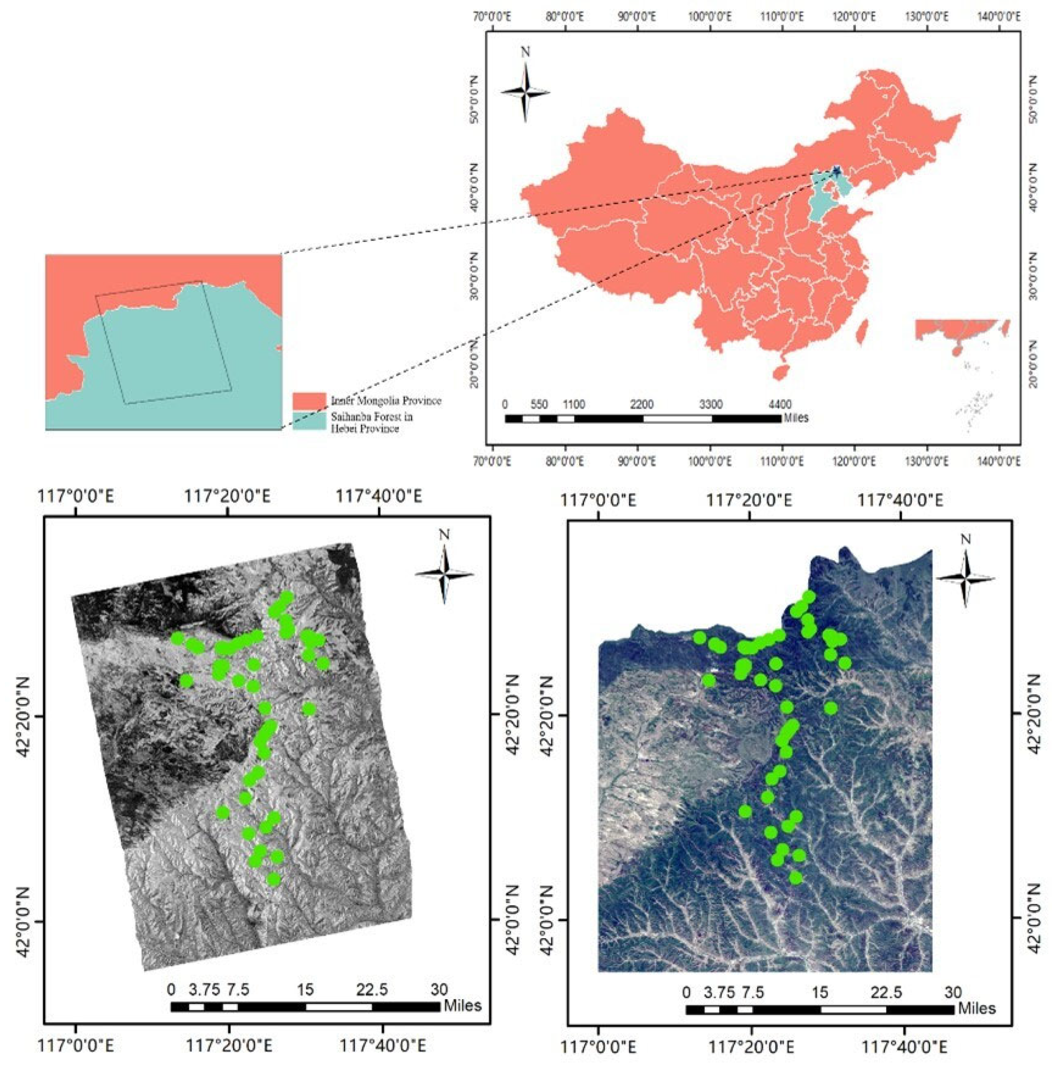
2.1. Study Area and Sample Data
2.2. Remote Sensing Data
2.2.1. Optical Data
2.2.2. SAR Data
3. Extraction of Variables
3.1. Extracting Information Based on Optical Data
3.1.1. Band
3.1.2. Texture
3.1.3. Biophysical Parameter (BP)
3.1.4. Horizontal Structure Index (HSI)
3.2. Extracting Information Based on SAR Data
3.2.1. Backscattering Coefficient (BC)
3.2.2. Polarization Decomposition Variable (PDV)
3.2.3. Polarization Decomposition Parameter (PDP)
3.2.4. SAR Index (SI)
3.2.5. Vertical Structure Index (H-VSI)
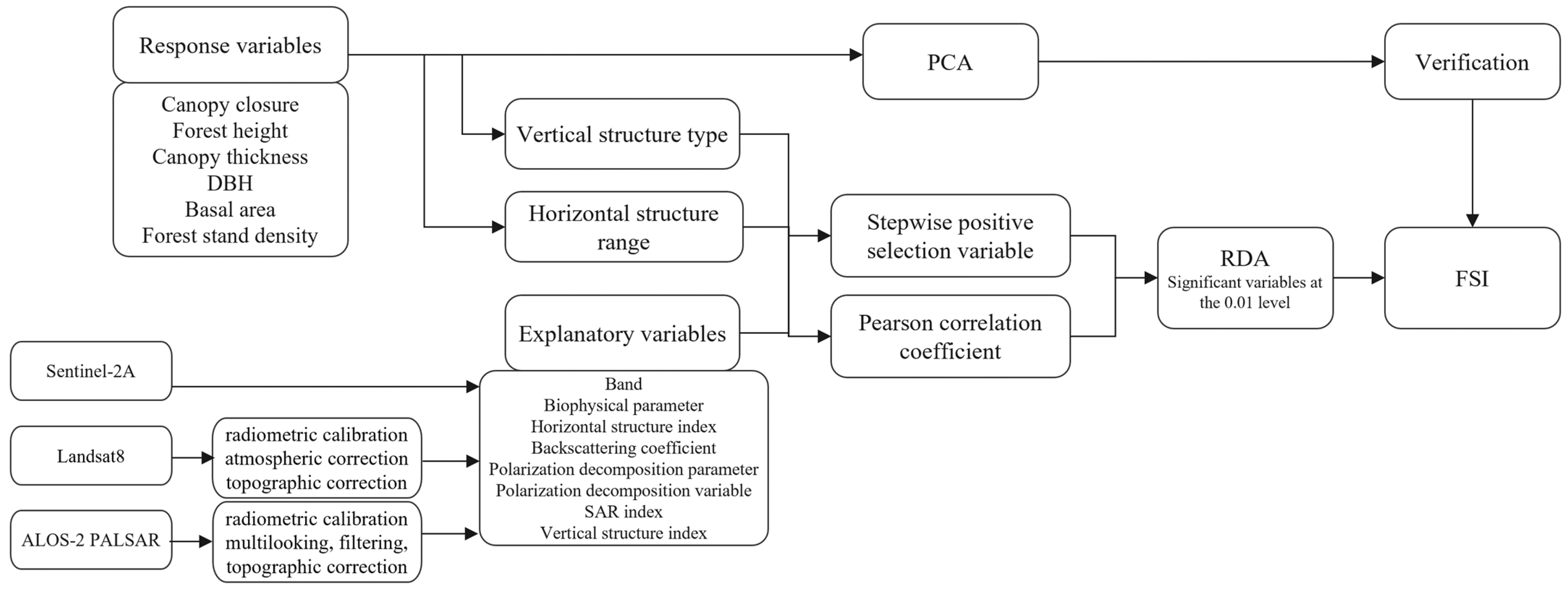
4. Proposed Method of the Research
4.1. Research Methods
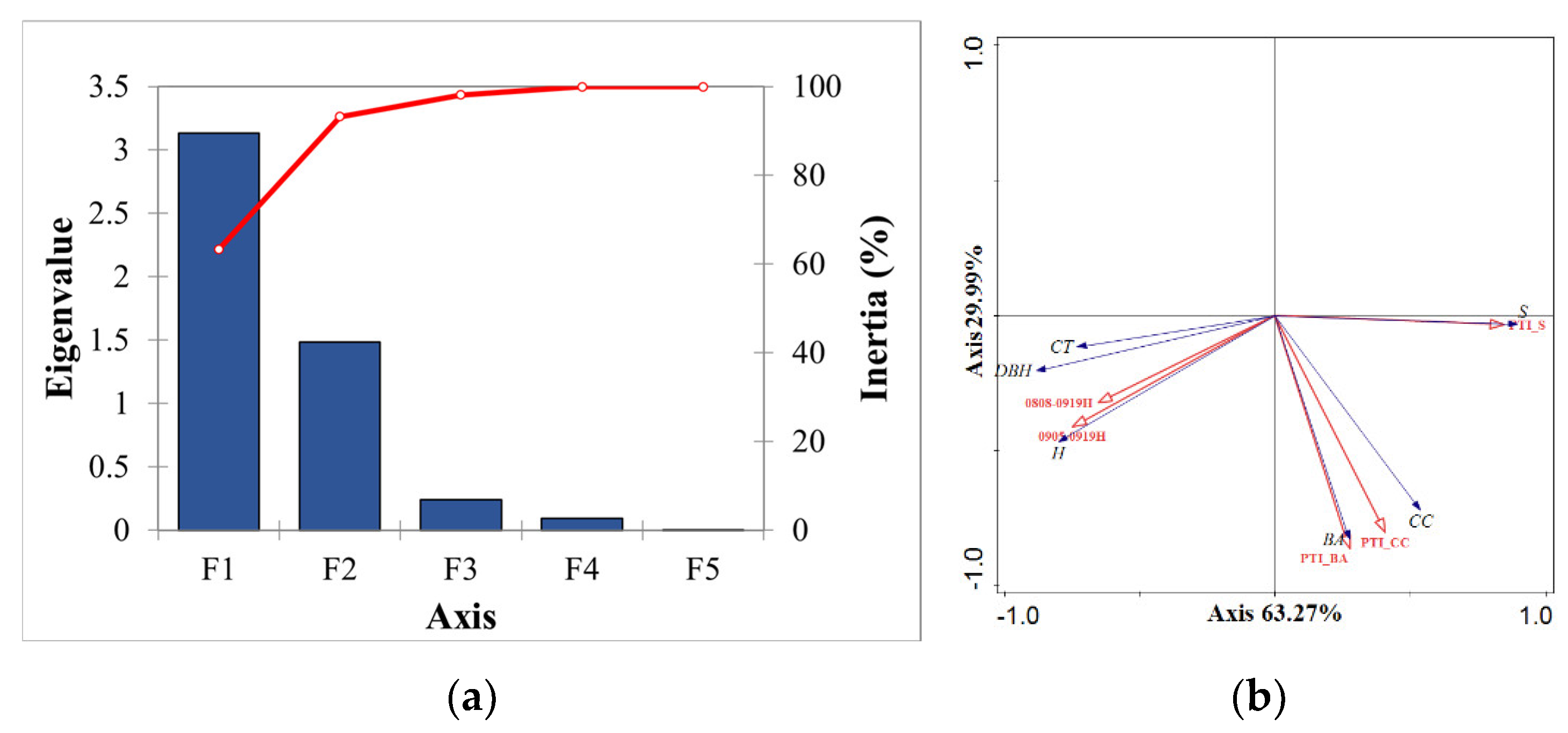
4.2. Redundancy Analysis (RDA)
5. Results
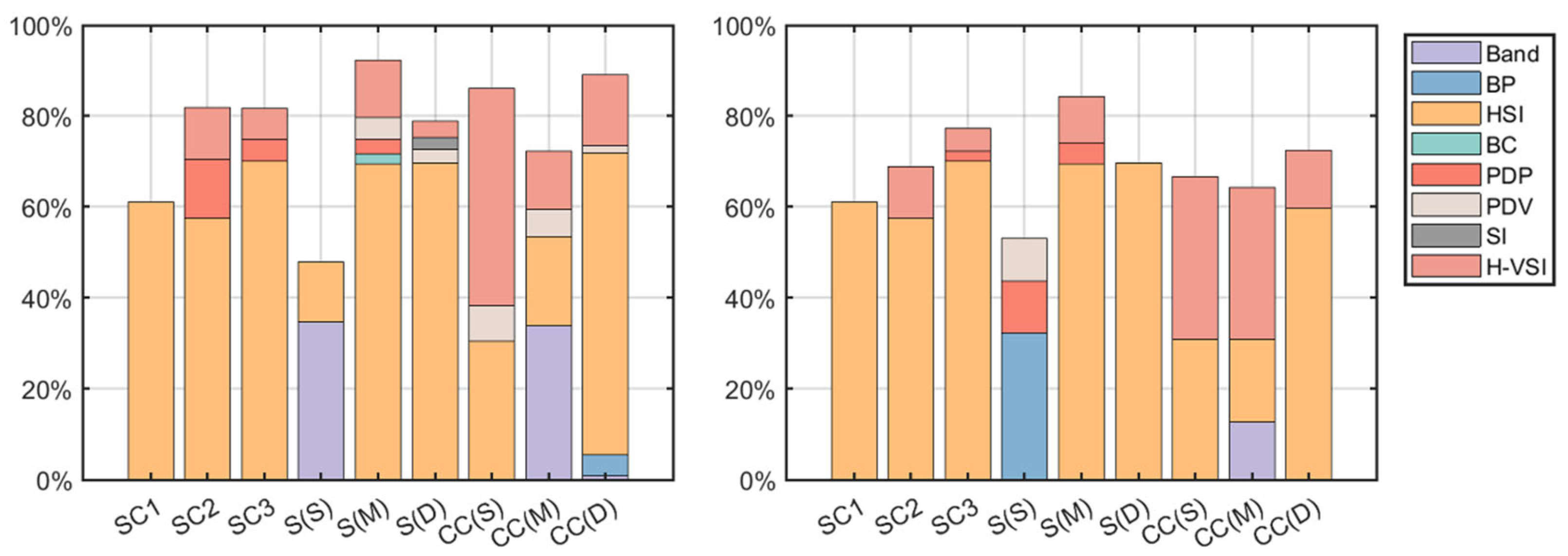
5.1. Selection Variables
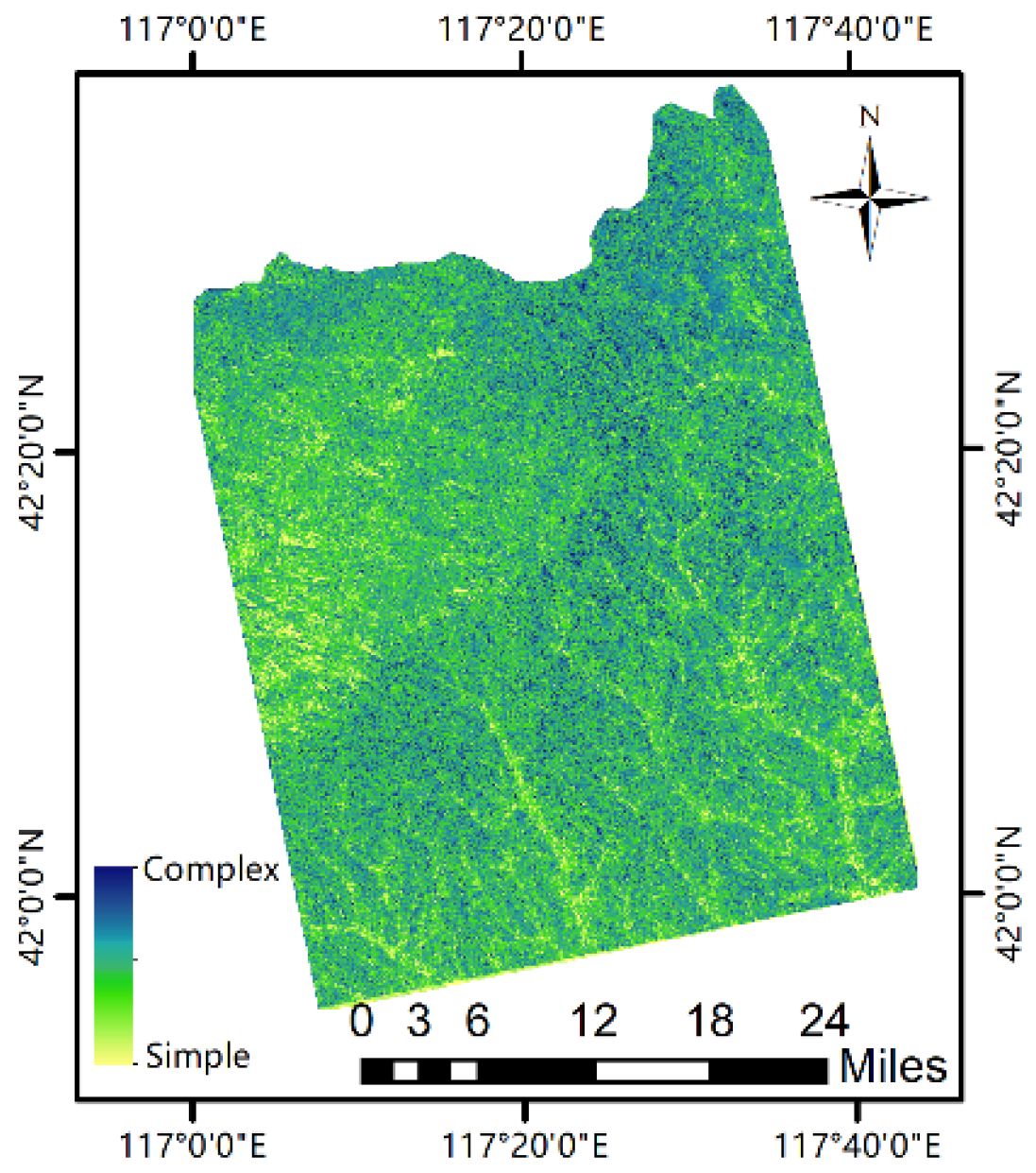
5.2. Establishment of the FSI Index
5.3. Validation of the FSI
6. Discussion
6.1. Stepwise Forward Selection of Variables
6.2. Pearson Correlation Coefficient Selection Variables
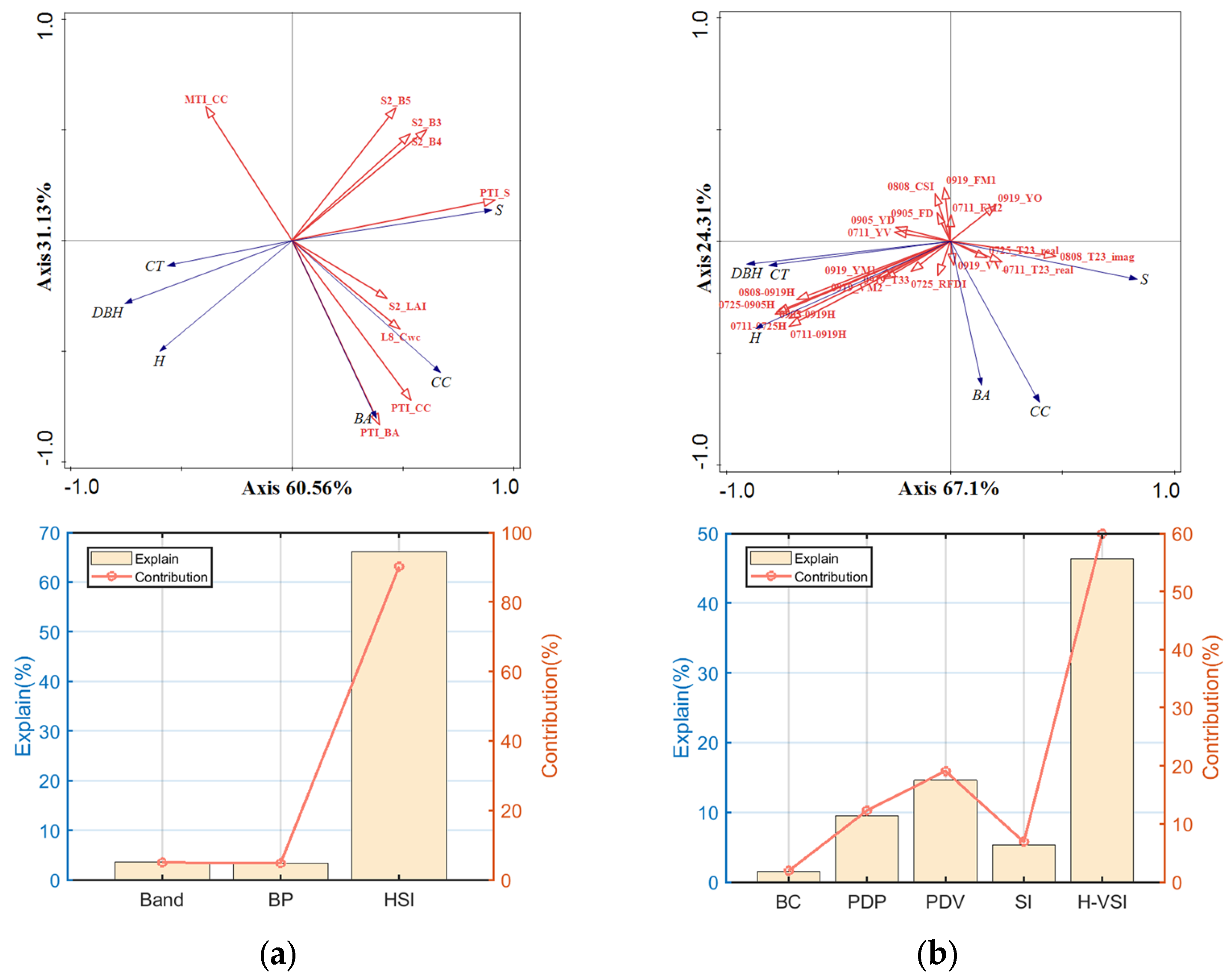
6.3. RDA for All Sample Plots
7. Conclusions
Supplementary Materials
Author Contributions
Funding
Data Availability Statement
Conflicts of Interest
Abbreviations
| Full Name | Abbreviation |
| ALOS-2 PALSAR | ALOS-2 |
| Basal area | BA |
| Backscattering coefficient | BC |
| Biomass index | BMI |
| Biophysical parameter | BP |
| Chlorophyll content in the leaf | Cab |
| Canopy closure | CC |
| Canonical correlation analysis | CCA |
| Canopy structure index | CSI |
| Mean canopy thickness | CT |
| corresponding texture index | CTI |
| Canopy water content | Cwc |
| Diameter at breast height | DBH |
| Freeman-Durden three-component decomposition | F |
| Forest structure index | FSI |
| Fractional Vegetation Cover | FVC |
| Mean forest height | H |
| Horizontal structure index | HSI |
| Vertical structure index | H-VSI |
| Landsat8 | L8 |
| Leaf Area Index | LAI |
| mean texture index | MTI |
| near-infrared | NIR |
| Principal component analysis | PCA |
| Polarization decomposition parameter | PDP |
| Polarization decomposition variable | PDV |
| Principal component texture index | PTI |
| Redundancy analysis | RDA |
| Radar forest degradation index | RFDI |
| Ratio texture index | RTI |
| Ratio vegetation index | RVI |
| Forest stand density | S |
| Sentinel-2A | S2A |
| Synthetic aperture radar | SAR |
| Structural complexity index | SCI |
| SAR Index | SI |
| Sehort-wave infrared | SWIR |
| Van Zyl decomposition | V |
| PTI_CC | V1 |
| PTI_S | V2 |
| PTI_BA | V3 |
| 0808-0919H | V4 |
| 0905-0919H | V5 |
| Volume scattering index | VSI |
| Yamaguchi three-component decomposition | Y |
References
- Chen, W.; Zheng, Q.; Xiang, H.; Chen, X.; Sakai, T. Forest Canopy Height Estimation Using Polarimetric Interferometric Synthetic Aperture Radar (PolInSAR) Technology Based on Full-Polarized ALOS/PALSAR Data. Remote Sens. 2021, 13, 174. [Google Scholar] [CrossRef]
- Franklin, J.F.; Spies, T.A.; Pelt, R.V.; Carey, A.B.; Thornburgh, D.A.; Berg, D.R.; Lindenmayer, D.B.; Harmon, M.E.; Keeton, W.S.; Shaw, D.C.; et al. Disturbances and structural development of natural forest ecosystems with silvicultural implications, using Douglas-fir forests as an example. For. Ecol. Manag. 2002, 155, 399–423. [Google Scholar] [CrossRef]
- Cazcarra-Bes, V.; Tello-Alonso, M.; Fischer, R.; Heym, M.; Papathanassiou, K. Monitoring of Forest Structure Dynamics by Means of L-Band SAR Tomography. Remote Sens. 2017, 9, 1229. [Google Scholar] [CrossRef]
- Keren, S.; Svoboda, M.; Janda, P.; Nagel, T. Relationships between Structural Indices and Conventional Stand Attributes in an Old-Growth Forest in Southeast Europe. Forests 2020, 11, 4. [Google Scholar] [CrossRef]
- Zenner, E.K.; Hibbs, D.E. A new method for modeling the heterogeneity of forest structure. For. Ecol. Manag. 2000, 129, 75–87. [Google Scholar] [CrossRef]
- Estes, L.D.; Reillo, P.R.; Mwangi, A.G.; Okin, G.S.; Shugart, H.H. Remote sensing of structural complexity indices for habitat and species distribution modeling. Remote Sens. Environ. 2010, 114, 792–804. [Google Scholar] [CrossRef]
- Sharma, R.C. Vegetation Structure Index (VSI): Retrieving Vegetation Structural Information from Multi-Angular Satellite Remote Sensing. J. Imaging 2021, 7, 84. [Google Scholar] [CrossRef]
- Banerjee, B.P.; Spangenberg, G.; Kant, S. Fusion of Spectral and Structural Information from Aerial Images for Improved Biomass Estimation. Remote Sens. 2020, 12, 3164. [Google Scholar] [CrossRef]
- Propastin, P. Modifying geographically weighted regression for estimating aboveground biomass in tropical rainforests by multispectral remote sensing data. Int. J. Appl. Earth Obs. Geoinf. 2012, 18, 82–90. [Google Scholar] [CrossRef]
- Wan, X.; Li, Z.; Chen, E.; Zhao, L.; Zhang, W.; Xu, K. Forest Aboveground Biomass Estimation Using Multi-Features Extracted by Fitting Vertical Backscattered Power Profile of Tomographic SAR. Remote Sens. 2021, 13, 186. [Google Scholar] [CrossRef]
- Tello, M.; Cazcarra-Bes, V.; Pardini, M.; Papathanassiou, K. Structural classification of forest by means of L-band tomographic SAR. In Proceedings of the 2015 IEEE International Geoscience and Remote Sensing Symposium (IGARSS), Milan, Italy, 26–31 July 2015; pp. 5288–5291. [Google Scholar]
- Cazcarra-Bes, T.; Papathanassiou, P. Assessment of forest structure estimation by means of SAR tomography: Potential and limitations. In Proceedings of the 2016 IEEE International Geoscience and Remote Sensing Symposium (IGARSS), Beijing, China, 10–15 July 2016. [Google Scholar]
- Pasher, J.; King, D.J. Development of a forest structural complexity index based on multispectral airborne remote sensing and topographic data. This article is one of a selection of papers from Extending Forest Inventory and Monitoring over Space and Time. Can. J. For. Res. 2011, 41, 44–58. [Google Scholar] [CrossRef]
- Lee, S.K.; Fatoyinbo, T.; Qi, W.; Hancock, S.; Armston, J.; Dubayah, R. Gedi and Tandem-X Fusion for 3D Forest Structure Parameter Retrieval. In Proceedings of the IGARSS 2018—2018 IEEE International Geoscience and Remote Sensing Symposium, Valencia, Spain, 22–27 July 2018; pp. 380–382. [Google Scholar]
- McElhinny, C.; Gibbons, P.; Brack, C.; Bauhus, J. Forest and woodland stand structural complexity: Its definition and measurement. For. Ecol. Manag. 2005, 218, 1–24. [Google Scholar] [CrossRef]
- Sharma, R.C.; Hara, K. Self-Supervised Learning of Satellite-Derived Vegetation Indices for Clustering and Visualization of Vegetation Types. J. Imaging 2021, 7, 30. [Google Scholar] [CrossRef] [PubMed]
- McElhinny, C.; Gibbons, P.; Brack, C. An objective and quantitative methodology for constructing an index of stand structural complexity. For. Ecol. Manag. 2006, 235, 54–71. [Google Scholar] [CrossRef]
- Wunderle, A.L.; Franklin, S.E.; Guo, X.G. Regenerating boreal forest structure estimation using SPOT-5 pan-sharpened imagery. Int. J. Remote Sens. 2007, 28, 4351–4364. [Google Scholar] [CrossRef]
- Olthof, I.; King, D. Development of a Forest Health Index Using Multispectral Airborne Digital Camera Imagery. Can. J. Remote Sens. 2000, 26, 166–176. [Google Scholar] [CrossRef]
- Cosmopoulos, P.; King, D.J. Temporal analysis of forest structural condition at an acid mine site using multispectral digital camera imagery. Int. J. Remote Sens. 2010, 25, 2259–2275. [Google Scholar] [CrossRef]
- Pasher, J.; King, D.J. Multivariate forest structure modelling and mapping using high resolution airborne imagery and topographic information. Remote Sens. Environ. 2010, 114, 1718–1732. [Google Scholar] [CrossRef]
- Torontow, V.; King, D. Forest complexity modelling and mapping with remote sensing and topographic data: A comparison of three methods. Can. J. Remote Sens. 2014, 37, 387–402. [Google Scholar] [CrossRef]
- Fischer, R.; Knapp, N.; Bohn, F.; Shugart, H.H.; Huth, A. The Relevance of Forest Structure for Biomass and Productivity in Temperate Forests: New Perspectives for Remote Sensing. Surv. Geophys. 2019, 40, 709–734. [Google Scholar] [CrossRef]
- Puliti, S.; Breidenbach, J.; Schumacher, J.; Hauglin, M.; Klingenberg, T.F.; Astrup, R. Above-ground biomass change estimation using national forest inventory data with Sentinel-2 and Landsat. Remote Sens. Environ. 2021, 265, 112644. [Google Scholar] [CrossRef]
- Chen, A.; Zebker, H. Reducing Ionospheric Effects in InSAR Data Using Accurate Coregistration. IEEE Trans. Geosci. Remote Sens. 2014, 52, 60–70. [Google Scholar] [CrossRef]
- Li, C.; Li, Y.; Li, M. Improving Forest Aboveground Biomass (AGB) Estimation by Incorporating Crown Density and Using Landsat 8 OLI Images of a Subtropical Forest in Western Hunan in Central China. Forests 2019, 10, 104. [Google Scholar] [CrossRef]
- Eckert, S. Improved Forest Biomass and Carbon Estimations Using Texture Measures from WorldView-2 Satellite Data. Remote Sens. 2012, 4, 810–829. [Google Scholar] [CrossRef]
- Li, C.; Zhou, L.; Xu, W. Estimating Aboveground Biomass Using Sentinel-2 MSI Data and Ensemble Algorithms for Grassland in the Shengjin Lake Wetland, China. Remote Sens. 2021, 13, 1595. [Google Scholar] [CrossRef]
- Zheng, H.; Cheng, T.; Zhou, M.; Li, D.; Yao, X.; Tian, Y.; Cao, W.; Zhu, Y. Improved estimation of rice aboveground biomass combining textural and spectral analysis of UAV imagery. Precis. Agric. 2019, 20, 611–629. [Google Scholar] [CrossRef]
- Solórzano, J.V.; Meave, J.A.; Gallardo-Cruz, J.A.; González, E.J.; Hernández-Stefanoni, J.L. Predicting old-growth tropical forest attributes from very high resolution (VHR)-derived surface metrics. Int. J. Remote Sens. 2017, 38, 492–513. [Google Scholar] [CrossRef]
- Gini, R.; Sona, G.; Ronchetti, G.; Passoni, D.; Pinto, L. Improving Tree Species Classification Using UAS Multispectral Images and Texture Measures. ISPRS Int. J. Geo-Inf. 2018, 7, 315. [Google Scholar] [CrossRef]
- Sharma, R.C. An Ultra-Resolution Features Extraction Suite for Community-Level Vegetation Differentiation and Mapping at a Sub-Meter Resolution. Remote Sens. 2022, 14, 3145. [Google Scholar] [CrossRef]
- Haralick, R.M.; Shanmugam, K.; Dinstein, I. Textural Features for Image Classification. IEEE Trans. Syst. Man Cybern. 1973, 6, 610–621. [Google Scholar] [CrossRef]
- Chen, L.; Wang, Y.; Ren, C.; Zhang, B.; Wang, Z. Optimal Combination of Predictors and Algorithms for Forest Above-Ground Biomass Mapping from Sentinel and SRTM Data. Remote Sens. 2019, 11, 414. [Google Scholar] [CrossRef]
- Weiss, M.; Baret, F.; Jay, S. S2ToolBox Level 2 Products LAI, FAPAR, FCOVER. [Research Report] EMMAH-CAPTE, INRAe Avignon. ⟨hal-03584016⟩. 2020. Available online: https://step.esa.int/docs/extra/ATBD_S2ToolBox_V2.0.pdf (accessed on 7 April 2024).
- Sa, R.; Fan, W. Estimation of Forest Parameters in Boreal Artificial Coniferous Forests Using Landsat 8 and Sentinel-2A. Remote Sens. 2023, 15, 3605. [Google Scholar] [CrossRef]
- Gitelson, A.A. Wide Dynamic Range Vegetation Index for remote quantification of biophysical characteristics of vegetation. J. Plant Physiol. 2004, 161, 165–173. [Google Scholar] [CrossRef] [PubMed]
- Nguy-Robertson, A.; Gitelson, A.; Peng, Y.; Viña, A.; Arkebauer, T.; Rundquist, D. Green Leaf Area Index Estimation in Maize and Soybean: Combining Vegetation Indices to Achieve Maximal Sensitivity. Agron. J. 2012, 104, 1336–1347. [Google Scholar] [CrossRef]
- Viña, A.; Gitelson, A. New developments in the remote estimation of the fraction of absorbed photosynthtically active radiation in crops. Geophys. Res. Lett. 2005, 32, L17403. [Google Scholar] [CrossRef]
- Chrysafis, I.; Mallinis, G.; Tsakiri, M.; Patias, P. Evaluation of single-date and multi-seasonal spatial and spectral information of Sentinel-2 imagery to assess growing stock volume of a Mediterranean forest. Int. J. Appl. Earth Obs. Geoinf. 2019, 77, 1–14. [Google Scholar] [CrossRef]
- Pourshamsi, M.; Xia, J.; Yokoya, N.; Garcia, M.; Lavalle, M.; Pottier, E.; Balzter, H. Tropical forest canopy height estimation from combined polarimetric SAR and LiDAR using machine-learning. ISPRS J. Photogramm. Remote Sens. 2021, 172, 79–94. [Google Scholar] [CrossRef]
- Alappat, V.O.; Joshi, A.K.; Krishnamurthy, Y.V.N. Tropical Dry Deciduous Forest Stand Variable Estimation Using SAR Data. J. Indian Soc. Remote Sens. 2011, 39, 583–589. [Google Scholar] [CrossRef]
- Khati, U.; Lavalle, M.; Singh, G. Spaceborne tomography of multi-species Indian tropical forests. Remote Sens. Environ. 2019, 229, 193–212. [Google Scholar] [CrossRef]
- Luckman, A.; Baker, J.; Kuplich, T.M.; da Costa Freitas Yanasse, C.; Frery, A.C. A study of the relationship between radar backscatter and regenerating tropical forest biomass for spaceborne SAR instruments. Remote Sens. Environ. 1997, 60, 1–13. [Google Scholar] [CrossRef]
- Cat, T.; Tani, H.; Wang, X.; Nguyen, T.; Bui, H. Combination of SAR Polarimetric Parameters for Estimating Tropical Forest Aboveground Biomass. Pol. J. Environ. Stud. 2020, 29, 3353–3365. [Google Scholar] [CrossRef]
- Wang, M.; Zhang, W.; Ji, Y.; Marino, A.; Xu, K.; Zhao, L.; Shi, J.; Zhao, H. Aboveground Biomass Retrieval in Tropical and Boreal Forests Using L-Band Airborne Polarimetric Observations. Forests 2023, 14, 887. [Google Scholar] [CrossRef]
- Xu, L.; Li, S.; Deng, Y.; Wang, R. Adaptive model-based scattering decomposition of Polarimetric SAR Interferometry. J. Electron. 2013, 30, 463–468. [Google Scholar] [CrossRef]
- Latrache, H.; Ouarzeddine, M.; Souissi, B. Improved model-based polarimetric decomposition using the polinsar similarity parameter. ISPRS-Int. Arch. Photogramm. Remote Sens. Spat. Inf. Sci. 2016, 41, 847–850. [Google Scholar] [CrossRef]
- Xie, Q.; Wang, J.; Liao, C.; Shang, J.; Lopez-Sanchez, J.; Fu, H.; Liu, X. On the Use of Neumann Decomposition for Crop Classification Using Multi-Temporal RADARSAT-2 Polarimetric SAR Data. Remote Sens. 2019, 11, 776. [Google Scholar] [CrossRef]
- Cui, Y.; Yamaguchi, Y.; Yang, J.; Park, S.-E.; Kobayashi, H.; Singh, G. Three-Component Power Decomposition for Polarimetric SAR Data Based on Adaptive Volume Scatter Modeling. Remote Sens. 2012, 4, 1559–1572. [Google Scholar] [CrossRef]
- Varghese, A.O.; Suryavanshi, A.; Joshi, A.K. Analysis of different polarimetric target decomposition methods in forest density classification using C band SAR data. Int. J. Remote Sens. 2016, 37, 694–709. [Google Scholar] [CrossRef]
- Golshani, P.; Maghsoudi, Y.; Sohrabi, H. Relating ALOS-2 PALSAR-2 Parameters to Biomass and Structure of Temperate Broadleaf Hyrcanian Forests. J. Indian Soc. Remote Sens. 2019, 47, 749–761. [Google Scholar] [CrossRef]
- Huynen, J. Phenomenological Theory of Radar Targets. Ph.D. Thesis, Delft University of Technology, Delft, The Netherlands, 1970. [Google Scholar]
- Zhu, Y.; Liu, K.; Myint, S.W.; Du, Z.; Li, Y.; Cao, J.; Liu, L.; Wu, Z. Integration of GF2 Optical, GF3 SAR, and UAV Data for Estimating Aboveground Biomass of China’s Largest Artificially Planted Mangroves. Remote Sens. 2020, 12, 2039. [Google Scholar] [CrossRef]
- Pope, K.O.; Rey-Benayas, J.M.; Paris, J.F. Radar remote sensing of forest and wetland ecosystems in the Central American tropics. Remote Sens. Environ. 1994, 48, 205–219. [Google Scholar] [CrossRef]
- Mitchard, E.; Saatchi, S.; White, L.; Abernethy, K.; Jeffery, K.; Lewis, S.; Collins, M.; Lefsky, M.A.; Leal, M.; Woodhouse, I.; et al. Mapping tropical forest biomass with radar and spaceborne LiDAR: Overcoming problems of high biomass and persistent cloud. Biogeosciences Discuss. 2011, 8, 179–191. [Google Scholar] [CrossRef]
- Sa, R.; Nei, Y.; Fan, W. Combining Multi-Dimensional SAR Parameters to Improve RVoG Model for Coniferous Forest Height Inversion Using ALOS-2 Data. Remote Sens. 2023, 15, 1272. [Google Scholar] [CrossRef]
- Mao, Y.; Michel, O.; Yu, Y.; Fan, W.; Sui, A.; Liu, Z.; Wu, G. Retrieval of Boreal Forest Heights Using an Improved Random Volume over Ground (RVoG) Model Based on Repeat-Pass Spaceborne Polarimetric SAR Interferometry: The Case Study of Saihanba, China. Remote Sens. 2021, 13, 4306. [Google Scholar] [CrossRef]
- Choi, C.; Pardini, M.; Heym, M.; Papathanassiou, K. Improving Forest Height-to-Biomass Allometry with Structure Information: A TanDEM-X Study. IEEE J. Sel. Top. Appl. Earth Obs. Remote Sens. 2021, 14, 10415–10427. [Google Scholar] [CrossRef]
- Fu, W.; Guo, H.; Song, P.; Tian, B.; Li, X.; Sun, Z. Combination of PolInSAR and LiDAR techniques for forest height estimation. IEEE Geosci. Remote Sens. Lett. 2017, 14, 1218–1222. [Google Scholar] [CrossRef]
- Aghabalaei, A.; Ebadi, H.; Maghsoudi, Y. Forest height estimation based on the RVoG inversion model and the PolInSAR decomposition technique. Int. J. Remote Sens. 2019, 41, 2684–2703. [Google Scholar] [CrossRef]
- Neumann, M.; Ferro-Famil, L.; Reigber, A. Estimation of Forest Structure, Ground, and Canopy Layer Characteristics From Multibaseline Polarimetric Interferometric SAR Data. IEEE Trans. Geosci. Remote Sens. 2010, 48, 1086–1104. [Google Scholar] [CrossRef]
- Deng, S.; Katoh, M.; Guan, Q.; Yin, N.; Li, M. Estimating Forest Aboveground Biomass by Combining ALOS PALSAR and WorldView-2 Data: A Case Study at Purple Mountain National Park, Nanjing, China. Remote Sens. 2014, 6, 7878–7910. [Google Scholar] [CrossRef]
- Pasher, J. Forest Structural Complexity in a Temperate Hardwood Forest: A Geomatics Approach to Modelling and Mapping Indicators of Habitat and Biodiversity. Ph.D. Thesis, Carleton University, Ottawa, ON, Canada, 2009. [Google Scholar]
- de la Cueva, A.V. Structural attributes of three forest types in central Spain and Landsat ETM+ information evaluated with redundancy analysis. Int. J. Remote Sens. 2008, 29, 5657–5676. [Google Scholar] [CrossRef]
- Sampson, P.H.; Treitz, P.M.; Mohammed, G.H. Remote Sensing of Forest Condition in Tolerant Hardwoods: An Examination of Spatial Scale, Structure and Function. Can. J. Remote Sens. 2014, 27, 232–246. [Google Scholar] [CrossRef]
- Dragozi, E.; Gitas, I.; Bajocco, S.; Stavrakoudis, D. Exploring the Relationship between Burn Severity Field Data and Very High Resolution GeoEye Images: The Case of the 2011 Evros Wildfire in Greece. Remote Sens. 2016, 8, 566. [Google Scholar] [CrossRef]
- Zhang, C.; Huang, C.; Li, H.; Liu, Q.; Li, J.; Bridhikitti, A.; Liu, G. Effect of Textural Features in Remote Sensed Data on Rubber Plantation Extraction at Different Levels of Spatial Resolution. Forests 2020, 11, 399. [Google Scholar] [CrossRef]
- Zhang, S.; Chen, H.; Fu, Y.; Niu, H.; Yang, Y.; Zhang, B. Fractional Vegetation Cover Estimation of Different Vegetation Types in the Qaidam Basin. Sustainability 2019, 11, 864. [Google Scholar] [CrossRef]
- Yongfeng, J. Estimation of Tree Biomass in Hubei Province by Coupling Optical Image Data and Topographic Factors. Master’s Thesis, Huazhong Agricultural University, Wuhan, China, 2021. [Google Scholar]
- Wang, Y.; Zhang, X.; Guo, Z. Estimation of tree height and aboveground biomass of coniferous forests in North China using stereo ZY-3, multispectral Sentinel-2, and DEM data. Ecol. Indic. 2021, 126, 107645. [Google Scholar] [CrossRef]


| Parameter | Max | Min | Mean | STD |
|---|---|---|---|---|
| CC (%) | 1 | 0.15 | 0.7 | 0.196 |
| H (m) | 27.8 | 5.81 | 17.3 | 4.88 |
| CT (m) | 17.9 | 4.6 | 9.5 | 2.8 |
| DBH (cm) | 33.1 | 7.2 | 22.74 | 7.3 |
| BA (m2/ha) | 48 | 1.2 | 24.7 | 9.7 |
| S (stems/ha) | 5100 | 133 | 960 | 1083 |
| Parameter | |
|---|---|
| Data Level | HBQR1.1 |
| Imaging Date | 0711, 0725, 0808, 0905, 0919 |
| Polarization Channel | Full polarization (HH, HV, VH, VV) |
| Master Image | Slave Image | Temporal Baseline (Days) | Vertical Wavenumber (rad/m) | Incidence Angle at the Scene Center (°) |
|---|---|---|---|---|
| 0711 | 0725 | 14 | 0.013–0.018 | 27.8054 |
| 0725 | 0808 | 14 | 0.010–0.015 | 27.8029 |
| 0905 | 0919 | 14 | 0.015–0.020 | 27.7991 |
| 0725 | 0905 | 42 | 0.010–0.016 | 27.8029 |
| 0808 | 0919 | 42 | 0.016–0.020 | 27.8012 |
| 0711 | 0919 | 70 | 0.019–0.027 | 27.8054 |
| Horizontal Structure | Dense | Medium | Sparse |
|---|---|---|---|
| S | |||
| CC |
| Variables | All (Times) | Significant (Times) /Percentage of Significant Times (%) | Variables | All (Times) /Percentage of Introduced Models (%) | Significant (Times) /Percentage of Significant Times (%) |
|---|---|---|---|---|---|
| Band | 35 | 3/9% | PTI_BA | 15/83% | 13/87% |
| BP | 21 | 2/10% | PTI_CC | 12/67% | 11/92% |
| HSI | 53 | 33/62% | 0808-0919H | 10/56% | 8/80% |
| BC | 16 | 0/0% | 0905-0919H | 8/44% | 4/50% |
| PDP | 35 | 10/29% | FM1 | 8/44% | 2/25% |
| PDV | 34 | 6/18% | PTI_S | 7/39% | 6/86% |
| SI | 14 | 1/7% | 0725-0905H | 6/33% | 0/0% |
| H-VSI | 37 | 17/46% | 0711-0725H | 3/17% | 1/33% |
| Ranking Axis | RDA1 | RDA2 | RDA3 | RDA4 |
|---|---|---|---|---|
| Eigenvalues | 3.131 | 1.483 | 0.240 | 0.092 |
| Explained variation (cumulative)/% | 52.18 | 76.9 | 80.9 | 82.44 |
| Pseudo-canonical correlation | 0.9585 | 0.9583 | 0.6868 | 0.6611 |
| Explained fitted variation (cumulative)/% | 63.27 | 93.26 | 98.11 | 99.97 |
| Variables | Explain | Contribution | Pseudo-F | Significance | RDA1 | RDA2 |
|---|---|---|---|---|---|---|
| V2 | 38.3 | 46.4 | 39.1 | 0.002 | 0.812 | −0.033 |
| V3 | 20.5 | 24.9 | 30.9 | 0.002 | 0.265 | −0.830 |
| V4 | 14.2 | 17.3 | 32.2 | 0.002 | −0.628 | −0.311 |
| V1 | 5.4 | 6.5 | 15 | 0.002 | 0.392 | −0.772 |
| V5 | 4 | 4.9 | 13.5 | 0.002 | −0.717 | −0.396 |
| KMO and Bartlett Test | ||
|---|---|---|
| KMO Measure of Sampling Adequacy | 0.699 | |
| Bartlett’s Test of Sphericity | Approx. Chi-Square | 317.366 |
| df | 15 | |
| Sig. | 0.000 | |
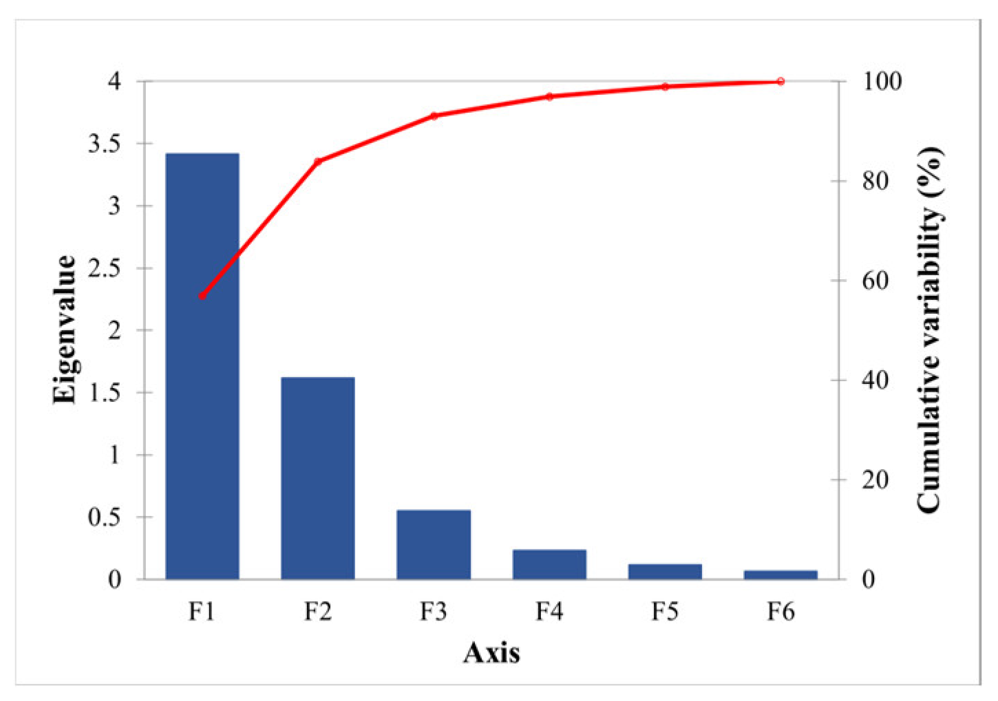
| Principal Component | PC1 | PC2 | PC3 |
|---|---|---|---|
| Eigenvalue | 3.414 | 1.617 | 0.552 |
| Variability (%) | 56.896 | 26.954 | 9.199 |
| Cumulative (%) | 56.896 | 83.849 | 93.049 |
| Eigenvalue | PC1 | PC2 | Loading Coefficients | PC1 | PC2 |
|---|---|---|---|---|---|
| CC | 0.281 | −0.602 | CC | 0.518 | −0.765 |
| H | −0.464 | −0.364 | H | −0.857 | −0.463 |
| CT | −0.444 | −0.127 | CT | −0.820 | −0.162 |
| DBH | −0.510 | −0.147 | DBH | −0.942 | −0.187 |
| BA | 0.140 | −0.679 | BA | 0.258 | −0.864 |
| S | 0.479 | −0.076 | S | 0.886 | −0.097 |
| Variables | All (Times) | Significant (Times) /Percentage of Significant Times (%) | Variables | All (Times) | Significant (Times) /Percentage of Significant Times (%) |
|---|---|---|---|---|---|
| Band | 13 | 3/23% | PTI | 19 | 16/84% |
| BP | 10 | 1/10% | H | 18 | 11/61% |
| HSI | 34 | 17/50% | D | 12 | 3/25% |
| BC | 13 | 1/8% | S2_Band | 11 | 3/27% |
| PDP | 26 | 7/27% | M1 | 9 | 2/22% |
| PDV | 30 | 6/20% | MTI | 7 | 1/14% |
| SI | 9 | 1/11% | M2 | 6 | 1/17% |
| H-VSI | 18 | 11/61% | CSI | 6 | 1/17% |
| VV | 5 | 1/20% | |||
| Cwc | 2 | 1/50% | |||
| T23_real | 2 | 2/100% |
| Variables | All (Times) | Significant (Times) /Percentage of Significant Times (%) | Variables | All (Times) | Significant (Times) /Percentage of Significant Times (%) |
|---|---|---|---|---|---|
| Band | 22 | 1/5% | H | 19 | 6/32% |
| BP | 11 | 1/9% | PTI | 16 | 14/88% |
| HSI | 20 | 16/80% | S2_Band | 16 | 1/6% |
| BC | 3 | 0/0% | T23_real | 5 | 2/40% |
| PDP | 9 | 3/33% | Cwc | 6 | 1/17% |
| PDV | 6 | 1/17% | M1 | 4 | 1/25% |
| SI | 8 | 0/0% | CTI | 2 | 1/50% |
| H-VSI | 19 | 6/32% | MTI | 2 | 1/50% |
Disclaimer/Publisher’s Note: The statements, opinions and data contained in all publications are solely those of the individual author(s) and contributor(s) and not of MDPI and/or the editor(s). MDPI and/or the editor(s) disclaim responsibility for any injury to people or property resulting from any ideas, methods, instructions or products referred to in the content. |
© 2024 by the authors. Licensee MDPI, Basel, Switzerland. This article is an open access article distributed under the terms and conditions of the Creative Commons Attribution (CC BY) license (https://creativecommons.org/licenses/by/4.0/).
Share and Cite
Sa, R.; Fan, W. Forest Structure Mapping of Boreal Coniferous Forests Using Multi-Source Remote Sensing Data. Remote Sens. 2024, 16, 1844. https://doi.org/10.3390/rs16111844
Sa R, Fan W. Forest Structure Mapping of Boreal Coniferous Forests Using Multi-Source Remote Sensing Data. Remote Sensing. 2024; 16(11):1844. https://doi.org/10.3390/rs16111844
Chicago/Turabian StyleSa, Rula, and Wenyi Fan. 2024. "Forest Structure Mapping of Boreal Coniferous Forests Using Multi-Source Remote Sensing Data" Remote Sensing 16, no. 11: 1844. https://doi.org/10.3390/rs16111844
APA StyleSa, R., & Fan, W. (2024). Forest Structure Mapping of Boreal Coniferous Forests Using Multi-Source Remote Sensing Data. Remote Sensing, 16(11), 1844. https://doi.org/10.3390/rs16111844