Abstract
In recent years, with the continuous development and popularization of unmanned aerial vehicle (UAVs) technology, the surge in the number of UAVs has led to an increasingly serious problem of illegal flights. Traditional acoustic-based UAV localization techniques have limited ability to extract short-time and long-time signal features, and have poor localization performance in low signal-to-noise ratio environments. For this reason, in this paper, we propose a deep learning-based UAV localization technique in low signal-to-noise ratio environments. Specifically, on the one hand, we propose a multiple signal classification (MUSIC) pseudo-spectral normalized mean processing technique to improve the direction of arrival (DOA) performance of a traditional broadband MUSIC algorithm. On the other hand, we design a DOA estimation algorithm for UAV sound sources based on a time delay estimation neural network, which solves the problem of limited DOA resolution and the poor performance of traditional time delay estimation algorithms under low signal-to-noise ratio conditions. We verify the feasibility of the proposed method through simulation experiments and experiments in real scenarios. The experimental results show that our proposed method can locate the approximate flight path of a UAV within 20 m in a real scenario with a signal-to-noise ratio of −8 dB.
1. Introduction
In recent years, thanks to the progress and development of science and technology, the use of unmanned aerial vehicles (UAVs) has expanded to many non-military fields, such as aerial photography, logistics, agricultural seeding, environmental monitoring, social security, and infrastructure maintenance [1,2]. This has also made the safety of UAVs a prominent social issue. The phenomena it leads to include, but are not limited to, drone theft, smuggling, and interference with aviation order [3,4]. In order to monitor UAVs in real time, anti-drone techniques have been introduced to counter drone attacks. Currently, the traditional method of localizing drones mainly utilizes RF radio technology [5,6,7], however, in some low signal-to-noise ratio (SNR) scenarios, the communication signal between the drone and the remote control can be interfered by the noise in the environment, resulting in a decrease in the localization accuracy or misjudgement of the UAVs as, for example, flying objects such as birds. Therefore, we urgently need a robust method for UAVs to perform localization work.
In terms of research related to UAV monitoring, one of the means of RF radio [5,6,7], radar [8,9], and image processing [10] is currently the main object of research, or a fusion between these research means [11,12]. RF radios are low-cost, can detect long distances, and the related technology is mature [13]. However, since the principle of RF radio detection is to extract features from the communication signals between the drone and the remote control, this method is influenced by the drone manufacturer, and the drone can be deliberately “silent” and not communicate with the remote control, which makes it difficult to locate the RF radio method. Radar, as a common means of airborne target monitoring, has obvious advantages. However, the “low, small, and slow” characteristics of UAVs have weakened these advantages to a certain extent; for example, radar can easily confuse UAVs with the same “low, small, and slow” birds [14]. Imagery means of localization are a related technology that is mature [15], covering a large variety of UAVs, and they have excellent localization and tracking performance; the disadvantage is that the effect is not good in the case of low visibility and obstacles.
Acoustic means of localizing UAVs using microphone arrays have unique advantages over traditional methods. They are independent of visibility and radio interference, low cost, easy to deploy quickly, and it is difficult for UAVs to “hide” the noise generated by the rotor blades. In particular, using acoustic means to localize UAVs has the unique advantage of working properly in harsh environments such as foggy days and dense electronic equipment, which has made them a mainstream method that has attracted the attention of many researchers in recent years. On the other hand, as the field of artificial intelligence continues to be hot in recent years, deep learning technology with its powerful feature extraction capability has also been applied by many scholars in the field of UAV acoustic source localization, and has gained performance improvements compared with the traditional acoustic source localization methods [16].
However, in the field of sound source localization for UAV noise, existing studies have not considered as much the problem of degradation of localization accuracy under a low signal-to-noise ratio. In the whole field of sound source localization, although existing studies have shown that deep learning techniques can guarantee good localization performance under low SNR conditions, most of these studies have focused on indoor speech localization for the human voice. In addition, the fast localization techniques based on arrival time differences are often used in UAV sound source localization, but their accuracy is still limited by the hardware sampling rate. Therefore, how to solve the above two difficult problems by technical means is research we need to carry out urgently.
Subject to the above analysis, we propose a UAV sound source localization technique in a low signal-to-noise ratio environment. Specifically, firstly, we design the microphone array layout after modeling and analyzing the sound field model for UAV sound source localization; then, we improve the traditional broadband MUSIC algorithm; secondly, we propose a DOA estimation algorithm for UAV sound source based on time delay estimation neural network; and lastly, we validate the validity of the proposed method in this paper through simulation and practical experiments. The contributions of this paper are as follows:
- Aiming at the poor performance of the traditional wideband MUSIC algorithm in estimating the DOA of UAV sound sources at low signal-to-noise ratios, we propose the MUSIC pseudo-spectral normalized mean processing technique to improve the DOA performance of the wideband MUSIC algorithm.
- Aiming at the problem that the DOA resolution of traditional time delay estimation algorithms is limited with poor performance under low signal-to-noise ratio conditions, we design a DOA estimation algorithm for UAV sound sources based on a time delay estimation neural network.
- In the experimental part, we compare the DOA algorithm performance with the localization simulation results through a large number of simulation experiments and actual experiments, respectively, as a way to verify the feasibility and robustness of the proposed method in this paper.
The rest of this paper is organized as follows. In Section 2, we introduce the related works to UAV localization. In Section 3, we introduce the microphone array signal processing technique, which consists of a microphone array signal model as well as a traditional DOA algorithm. In Section 4, we propose a DOA algorithm based on normalized mean pseudo-spectral MUSIC and a DOA algorithm for UAV sound sources based on a time delay estimation neural network, and provide a detailed theoretical derivation and feasibility illustration of the proposed methods. In Section 5, we verify the feasibility of the proposed methods in this paper through simulations and practical experiments. Finally, Section 6 summarizes the whole paper.
2. Related Works
Currently, most hardware implementations of sound source localization use microphone arrays [17]. The microphones are arranged according to a specific way, and the arrangement is usually known, so the signals received by multiple microphones can be processed based on the known information about the arrangement to obtain information about the position of the sound source in space.
The principles of microphone array signal processing are similar to those of array signal processing used by radar and sonar, but there are some differences. Radar and sonar usually target one or more narrowband signals, while the audio received by microphones is usually a non-smooth broadband signal. Microphone array source localization techniques can be classified into three categories based on their principles [18]: beam shaping based on maximum output power, super-resolution estimation, and localization techniques based on time-difference-of-arrival (TDOA) estimation.The generalized mutual correlation phase transform method proposed by Knapp and Carter is still the most commonly used method for TDOA estimation [19]. DiBiase et al. improved the performance of the generalized correlation method for TDOA estimation in indoor reverberant environments by increasing the number of microphones [20]. However, since the accuracy of TDOA estimation is directly related to the sampling rate, the final localization performance is also limited by the sampling rate determinism. The super-resolution estimation class of localization techniques breaks through the sample rate limitation. Dmochowski et al. extended the classical method MUSIC for narrowband source localization to broadband signals, making it usable for sound source localization [21]. However, such methods are computationally intensive and are not favorable for deployment on small-sized hardware [17]. In summary, sound source localization techniques via microphone arrays also have their limitations.
In recent years, the potential of data-driven deep learning techniques to address various limitations in sound source localization has attracted the interest of researchers. Chakrabarty and Habets showed that the use of convolutional neural networks can lead to a twofold improvement in overall localization accuracy over the use of conventional methods under low signal-to-noise ratio conditions [22]. Perotin et al. proposed the use of convolutional recurrent neural networks instead of the traditional independent component analysis-based approach to improve the localization accuracy by 25% [23]. Advanne et al. used convolutional recurrent neural networks instead of eigenvalue decomposition in the traditional super-resolution estimation to bypass the complex computation and experimentally demonstrated that the average error of the proposed scheme under reverberant conditions was improved compared to the traditional MUSIC reduced by half [24]. VeraDiaz designed an end-to-end convolutional neural network for sound source localization, the input of the network is the original audio signal and the output is the 3D spatial Cartesian coordinates, and the experimental results show that the localization of indoor speech using the proposed network is better than the traditional methods [25]. Salvati et al. used a convolutional neural network to improve the performance of traditional TDOA for indoor speech localization [26]. DiazGuerra et al. applied a 3D convolutional layer on a controlled response power map for calculating azimuth and pitch angles and designed the entire localization system to operate in a fully causal mode to be able to use it in real time [27].
Sound source localization for UAV noise is a relatively new field and some studies have been carried out in recent years. The team at Wright State University (USA) earlier proposed the use of microphone arrays for sound source localization of UAVs in both traditional time-of-arrival difference estimation and beam fouling [28]. Purdue University and Wright State University also used the same classification problem modeling approach in the literature [29], and implemented a real-time runnable UAV acoustic localization system on a Raspberry Pi using a model combining time-frequency diagrams and support vector machines. A team from Zhejiang University in China designed a microphone array-based UAV localization system, which uses a Bayesian filter-optimized TDOA estimation algorithm to ensure good UAV localization performance [30].
In the above research on sound source localization for UAV noise, not many scholars have paid attention to the effect of the bias of localization results in low signal-to-noise ratio environments. After the introduction of deep learning technology, although the accuracy is improved, the prediction accuracy of its network is still affected by the quality of the dataset. Based on the above analysis, this paper proposes a deep learning-based sound source localization technique for UAVs under low signal-to-noise ratio conditions, which ensures the accuracy of the localization results while possessing the robustness of the localization model.
3. Microphone Array Signal Processing Technology
In this section, we model the microphone array signal and introduce the traditional DOA algorithm.
3.1. Microphone Array Signal Model
In general, the scenario monitored by the UAV meets the far-field single-source condition, which is illustrated in Figure 1: counting the first microphone from right to left as a reference, the signal received by the second microphone at time point k is:
where a is the acoustic air propagation attenuation coefficient, t is the length of time it takes for the signal to travel from the acoustic source to the reference microphone, is the time delay between the second microphone and the reference microphone, and is the external noise at the second microphone. Since the source and the two microphones are in the same plane, the normal of the far-field acoustic signal wavefront is at an angle of to the line connecting the two microphones. Taking the received signal on the right as the reference signal, the received by the left microphone is delayed by (c is the speed of sound in the air) with respect to the , so that the time delay between the two microphones is:
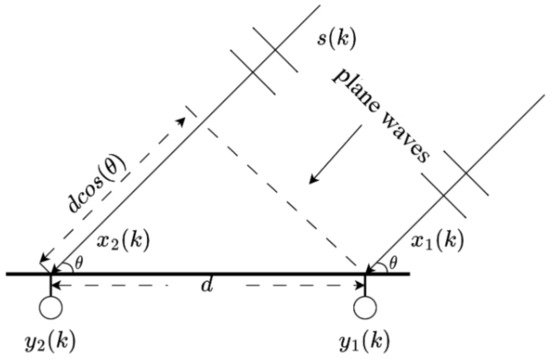
Figure 1.
Schematic of direction of arrival estimation for a single source in the far field with two microphones in the same plane.
It should be noted here that due to the limitation of the microphone spacing d, the delay takes values in the range of , . Equation (1) can be generalized when there are not only two but N microphones forming a uniform line array:
where , and represent the delay between the nth microphone and the first microphone (reference microphone). Therefore, we only need to determine the time delay value for the direction of the arrival angle .
3.2. Conventional DOA Algorithm for Microphone Arrays
As with conventional array signal processing, the DOA used in microphone array signal processing is broadly categorized into three types: intercorrelation-based delay estimation, beam fouling, and super-resolution estimation.
3.2.1. Intercorrelation-Based Delay Estimation
Under far-field conditions, the angle can be found by substituting into Equation (2) as long as the time delay is estimated. Correlation is the most intuitive way to estimate the time delay of two discrete signals. Also consider the simple model shown in Figure 1. We define the correlation between the two signals and as:
Typically, since there is no correlation between the source signal and the noise received by the microphone, there is no correlation between the noise and received by the respective microphones. And, when p = , obtains the maximum value. Thus, the time delay between the two microphones can be obtained as:
where . However, in real-world environments, the signal-to-noise ratio of sound source localization scenarios is usually less than ideal, which makes direct mutual correlation less effective. Generalized inter-correlation [19] is a method to improve the performance of inter-correlation at low signal-to-noise ratios by sharpening its spikes. Since the autocorrelation of the signals is Fourier transformed into pairs with the spectrum, and the mutual correlation of the two signals with the reciprocal spectrum also holds when replaced, it is obtained:
where denotes the Inverse Discrete Fourier Transform (IDFT), is the weighting function, and denotes the inter-frequency spectrum. The generalized mutual correlation method can choose the weight function according to different needs [31]. The multiplication of the weighting function with the mutual spectrum is called the generalized mutual spectrum. From the above equation, it can be seen that the key to delay estimation lies in the phase information in the inter-frequency spectrum, and the amplitude information in the spectrum is independent of the delay. Therefore, we can perform normalization of the spectral magnitude such that the weight function:
We can obtain the phase transform method. At this point, the generalized reciprocal spectrum , whose value depends only on the time delay . Then, substitute into Equation (7) to obtain:
It can be seen in Equation (9) that the spikes of the correlation are theoretically infinite. Of course, in real scenarios, due to the presence of noise, spikes cannot be infinite, and beyond that the spikes cannot be 0, but this has served to sharpen the spikes, which is the GCC-PHAT method. It can estimate the delay in a very short time and has some noise immunity. The disadvantage of this method lies mainly in the indoor source localization scenario, which is due to the reverberant nature of the indoor sound field.
3.2.2. Beam Fouling
In real-world environments, the angle of incidence of signals of different frequencies on the same microphone array varies, even if they are emitted from the same location. Delayed summation works well for narrowband signals with a single frequency, however, it is greatly affected by sources belonging to broadband signals. Thus, for broadband signals, we propose a filter-summing method, which is an improved beam fouling method based on delay summation. The key lies in the subband decomposition of the full-frequency domain, and then the design of the respective delay-summing beams in different subbands, which is equivalent to turning the original spatial filter into a space-time filter, thus realizing the frequency-invariant spatial response characteristics of the array. The mathematical expression of the filter summing beam assignment in the frequency domain is:
where is the weight function and the independent variable t is the representation of the time domain to be taken into account in the filter-summing process. For microphone arrays for any point in space, we combine the filter-summing beam assignment with generalized inter-correlation to propose the Steerable Response Power method (SRP). First, the generalized mutual correlation of all Mic-Pairs of the signal at this point is picked up, and then the spatial spectrum is traversed over the angles to be localized, and the maximum point of the computed value is the orientation of the source. SRP can be derived using the output power of the filter-summing beam farming:
Equation (11) represents the controllable response power over a particular angle space at a particular moment in time, and when the respective filter weights of the filter summation beam assignment are determined as in Equation (11), the SRP is only related to the direction of arrival . Substituting Equation (10) into Equation (11):
Note that since the moments are already specific, this side does not consider omitting the independent variable t in the original equation. p and q in Equation (12) represent the two microphone signals, respectively, and is actually the interrelationship between the two signals of the two p and q . The time delay represented by this mutual correlation spike corresponds to a certain azimuthal angle in space , so the SRP is the sum of the generalized mutual correlations of all microphone pairs:
When the weight function , this is the phase transform of the SRP, called SRP-PHAT.
3.2.3. Super-Resolution Estimation
Super-resolution estimation was initially proposed in the theory of conventional array signals such as radar, and has since been extended to the field of broadband signals processed by microphone arrays. We introduce the MUSIC based on Subspace Decomposition method [32]. First, the concept of arrival vector needs to be introduced first.
In a uniform line array with a total of M array elements, assuming that the source signal received by the reference array element is , then the source signal received by the Nth array element is , which has a power spectral density of:
Thus, the frequency domain form of the M array element uniform line array received signal model is:
where the elements in are the arrival vectors, which are also called orientation vectors. The time domain expression of Equation (15) can be written as:
where is the source signal and is the noise. A is known as the streaming matrix, which consists of arrival vectors. The arrival vector contains the relative phase shift of the plane wave radiated from a particular source at the location of the array, and each array element has a corresponding arrival vector. The key to the subspace decomposition is the covariance matrix of the array, which is obtained from the array received signal, that is, in Equation (16). When is uncorrelated with , it is possible to decompose :
We perform an eigenvalue decomposition of and let the rank of be D, then it has D positive real eigenroots and zero eigenroots (M is the number of array elements). The positive real eigenroots are related to the signal, and their corresponding eigenvectors constitute the signal subspace ; the zero eigenvalues are not related to the signal and their corresponding eigenvectors constitute the null subspace . Since the feature roots in the null subspace are orthogonal to the feature roots in the signal subspace, and the arrival vectors belong to the signal subspace, the feature roots in the null subspace are also orthogonal to the arrival vectors, i.e., .
When noise is considered, the null subspace becomes a noise subspace. The MUSIC algorithm is based on the noise subspace to construct a power function with the direction of arrival as the independent variable, called the pseudo-spectrum, whose mathematical expression is:
When the arrival vector is perfectly orthogonal to the noise subspace, the spikes in the pseudo-spectrum will tend to infinity. However, in the real environment due to the noise must exist (microphone itself has noise), the arrival vector can not be completely orthogonal to the noise subspace, so the maximum value in the pseudo-spectrum is finite, and its corresponding independent variable is the result of the arrival direction estimation. Finally, the DOA can be found by utilizing the following equation:
4. Our Methods
On land, the layout of the microphone array has a significant impact on the accuracy and reliability of sound source localization. At the same time, noise in urban environments adversely affects the transmission and acquisition of acoustic signals, making the signal-to-noise ratio very low, which decreases the accuracy of localizing the target sound source. In this chapter, the microphone array layout is designed after analyzing the sound field model for UAV sound source localization. Then, the traditional wideband MUSIC algorithm is improved to address the problem of deterioration of the DOA estimation of the UAV sound sources under low SNR conditions. Finally, the DOA estimation algorithm for UAV sound sources based on the time delay estimation neural network is proposed to address the problem of limited DOA resolution and poor performance under the low signal-to-noise ratio of the traditional time delay estimation algorithm.
4.1. Problems Description and Analysis
4.1.1. Sound Field Modeling
Currently, the mainstream use of microphone arrays to localize the sound source can be divided into two steps: 1. Direction of Arrival Estimation (DOA) and 2. using the triangular geometric relationship of the angle estimated by DOA to localize, while the first step is mainly for the far-field signal. Like conventional array signals, microphone array signals are divided into far-field and near-field models. The difference between the two is that under far-field conditions, the amplitudes of signals from different microphones picking up the same source are considered to be the same, differing only in phase, i.e., the sound wave propagates in the form of a plane wave; under near-field conditions, the amplitudes of signals from different microphones picking up the same source have their own attenuation. When the shape of the microphone array is a uniform line array, define as the distance from the sound source to the midpoint of the array, L as the total length of the array, and as the wavelength of the propagating sound wave. When these parameters satisfy Equation (20) [33], the sound source localization scenario meets the far-field condition.
It is assumed that a uniform line array of microphones with a total length of 1 m is deployed on the ground, i.e., L = 1. The frequency interval taken for sound source localization of UAVs in the literature [34] is from 309 Hz to 3400 Hz. In order to keep the wavelength as short as possible, we take the highest frequency of 3400 Hz, which corresponds to a wavelength of 0.1 m in the air. According to the above equation, when the distance of the two-element microphone line array is greater than 5 m, it meets the far-field condition. The UAV must be a certain distance away from the microphone array to have the value of detection, so this paper subsequently applies the microphone far-field reception model to the UAV sound source localization scenario.
In the microphone array far-field reception model, the DOA of each array element is theoretically the same. In other words, the DOA direction of each microphone is located in a straight line parallel to each other, and the parallel lines have no intersection point, it is impossible to determine the specific coordinates. It is then necessary to estimate another DOA with another array B (call the first array A), and this DOA is not the same as the DOA of array A. Then, we can get two non-parallel straight lines, and their intersection point is the position of the sound source. It should be noted that such a localization algorithm requires that the spatial coordinates of arrays A and B are known. In a real scenario, the arrays are usually arranged by human beings, and the natural spatial coordinate information is known.
4.1.2. Microphone Array Construction
Essentially, this section utilizes two independent uniform line arrays as equivalent subarrays to form a large equivalent sparse line array. This is shown in Figure 2.
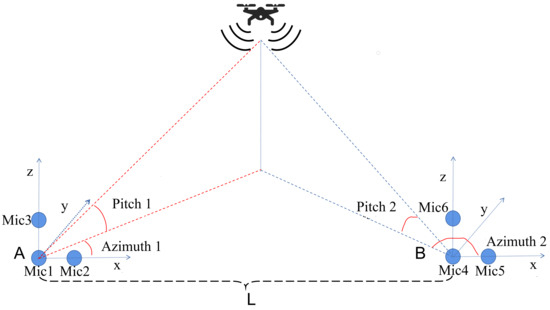
Figure 2.
Schematic of the microphone array for localizing the sound source of the UAV.
Figure 2 shows two arrays of six microphones. Unlike the previous discussion of DOA, which is limited to the 2D plane, in the actual scenario, 3D spatial localization is required, so Mic1, Mic3, Mic4, and Mic6 in the figure constitute two line arrays perpendicular to the x–y plane (ground), and their estimated DOA is used as the elevation. Mic1, Mic2, Mic4, and Mic5 are responsible for estimating two different azimuth angles to localize the projection of the UAV sound source on the ground.
4.2. Doa Algorithm Based on Normalized Mean Pseudo-Spectrum MUSIC
UAV sound sources are broadband signals that contain multiple frequency components and the signal subspaces are different for different frequency signals. The performance of the MUSIC algorithm described in the previous section is greatly degraded in such cases. If the MUSIC algorithm is to be extended to the field of broadband signals, the traditional approach is to divide the broadband into several sub-narrowbands, then perform narrowband MUSIC-DOA in each sub-narrowband, and finally fuse the DOA results of all sub-narrowbands, which is known as the full-frequency fusion MUSIC algorithm. The disadvantage of this algorithm is that it does not take into account that the signal-to-noise ratio is different in different sub-narrow bands. Because, for example, the energy of the drone sound source is concentrated in several of the sub-narrow bands, and the energy in the other sub-narrow bands is negligible, which leads to a large deviation between the DOA estimation results of each sub-narrow band, and it is difficult to make the fused DOA accurate [35].
To address this, following the idea of the generalized correlation-phase transform, this section builds on the pseudo-spectrum shown in Equation (18). By normalizing the spectral amplitude at each frequency point, the contributions to the DOA from the energy from the source and from the noise energy in each sub-narrow band are not affected by the respective power spectral amplitudes, thus enhancing the robustness of the final DOA fusion result.
According to Equation (15), it is known that the arrival vector is related to the angular frequency w and the time delay , so the arrival vector in Equation (18) can be rewritten as to to obtain:
As we discussed in the previous section, the relative time delay between the two microphones . In the actual localization scenario, on the other hand, we acquire discrete digital signals, which means that the interval is not a continuous line, but rather a series of discrete dots, and the spacing between the dots depends on the microphone’s sampling rate . We can write this using Equation (2):
It should be noted that essentially represents a sampling point at a moment in time, so it does not have a unit of time like , which has to be multiplied by the sampling rate in order to represent the duration. On the basis of Equation (21) and the fact that is a series of integer values, it is possible to construct the vector , called the omnidirectional power vector.
Next, the pseudo-spectrum calculation as shown in Equation (21) is first performed within each sub-narrowband, and then the pseudo-spectrum is normalized by the vector with the largest mode in the omni-directional power vector, and finally the normalized sub-narrowband pseudo-spectrums are combined into the total broadband pseudo-spectrum. The specific processing flow in practice is as follows:
- Input an audio matrix, where M is the number of microphones and T is the length of a single channel of audio.
- For each column vector of the audio matrix in the first step is calculated;
- For each column corresponding to , the eigenvalues are used to decompose the noise subspace ;
- Using the noise subspace from step 3 and Equation (21), compute ;
- For , the omnidirectional power vector is computed first, then ;
- Repeat step 5 for ;
- The results obtained in steps 5 and 6 are concatenated into vectors to obtain the total pseudo-spectrum;
- The frequency axis of the total pseudo-spectrum is converted to an angular axis using for spectral peak search.
Figure 3 and Figure 4 shows the improvement of the normalized mean for the MUSIC spatial power spectrum spikes. In this simulation, the receiving array is a binary microphone line array with a spacing of 0.5 m between the array elements, and the source is 10 m away from the array. The source signal is an audio sample of a drone noise from the [18] dataset, with an incoming wave direction of 80°, additive noise, and a signal-to-noise ratio of 0 dB. In Figure 3, the sharpest peak is in the 80° direction, however, there is also a sharper peak in the 140° direction and three more distinct peaks in other directions. Next, the signal-to-noise ratio is further reduced and the other parameters are kept constant and the simulation is performed again.
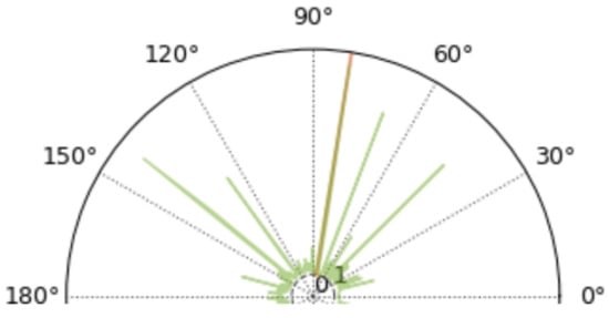
Figure 3.
MUSIC spatial power spectrogram.
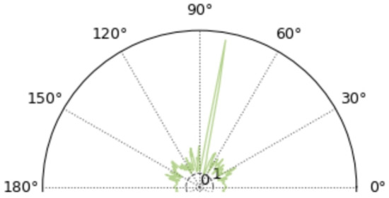
Figure 4.
Normalized mean MUSIC spatial power spectrogram.
The simulation presented in Figure 5 and Figure 6 shows a decrease in signal-to-noise ratio from 0 dB to −5 dB compared to Figure 3 and Figure 4. It can be found that in the MUSIC spatial power spectrum shown in Figure 5, although there are still sharp peaks in the 80° direction, the DOA estimation becomes more than 150° due to the fact that there are peaks around 155° that are slightly sharper than those in the 80° direction. In contrast, the normalized-mean-processed MUSIC spatial power pseudo-spectrum illustrated in Figure 5 and Figure 6 still has only one sharp spectral peak. Compared with Figure 4, the overall power in Figure 5 and Figure 6 becomes larger in all other directions, but there is no obvious spectral peak. It can be shown that the algorithm of normalized averaging on top of the MUSIC pseudo-spectrum improves the robustness of the DOA in the case of low signal-to-noise.
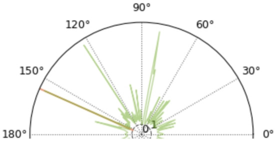
Figure 5.
MUSIC spatial power spectrogram.
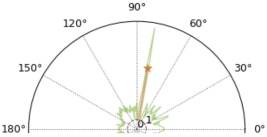
Figure 6.
Normalized mean MUSIC spatial power spectrogram.
4.3. DOA Algorithm for UAV Sound Source Based on Time Delay Estimation Neural Network
In the previous section, the algorithm based on MUSIC super-resolution estimation has achieved good results, however, it is computationally intensive considering that it requires the calculation of autocorrelation as well as omnidirectional power vectors frequency by frequency, and there is also a matrix-specific value decomposition step. In addition, the accuracy of the MUSIC algorithm localization is theoretically related to the number of snapshots, the larger the number of snapshots, the more accurate, but this also means that the signal duration is larger, resulting in the inability of fast localization.
In sound source localization, an algorithm that directly estimates the delay using GCC-PHAT is very popular. This algorithm is computationally small and fast in judgment. However, in real scenarios, this algorithm is also subject to certain constraints. The resolution of its DOA is affected by the sampling rate, and at the same time, the delay estimation in low signal-to-noise ratio environments is prone to errors. To address the above problems, this section proposes a DOA algorithm for delay estimation based on convolutional neural networks.
4.3.1. Modeling the Delay Estimation Problem
As discussed in Section 2, the PHAT weighting function determines the effect of amplitude on whitening in the spectrum. This effect, if appropriate, can reduce the noise energy in certain spectral components where the signal-to-noise ratio is low. We use a parameter to denote different degrees of PHAT weighting functions in GCC-PHAT, which can be written from Equations (7) and (8):
where . Since we are actually dealing with discrete digital signals, Equation (23) is rewritten for ease of presentation:
where k is the index of each sampling point. The matrix is constructed according to Equation (24):
where are the different parameter values, B is the total number of parameters, and . Our next task is to design a nonlinear function , which is a parameter that will be automatically updated through learning in the neural network. The effect of this nonlinear function is to establish a mapping between the matrix shown in Equation (25) and the time delay , which is the correct value of the time delay that corresponds to the direction of the incoming wave from the source, and so there is:
The above equation is the model we are going to implement using deep learning, with being the input and being the output.
4.3.2. Delay Estimation Network Construction
The entire structure of our proposed network consists of convolutional layers except for the final fully connected layer. Unlike the use of deep neural networks for drone noise recognition, here the output layer of the network is regressed without classification. The Root Mean Square Error (RMSE) is used as the loss function in the training process and its mathematical expression is:
where is the network prediction, is the ideal prediction, and N is the number of predictions. Figure 7 illustrates the convolutional neural network architecture employed for the construction of Equation (26). In order to enhance the nonlinearity of the model as well as to reduce overfitting during training, two dropout layers with a dropout probability of 0.2 were added to the three fully connected layers. The horizontal and vertical step size of each convolutional layer in the network is 1, and padding is specified as the same mode.
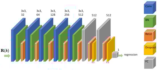
Figure 7.
Our convolutional neural network architecture.
4.3.3. Network Training
The sound source was the drone noise audio from [18], and the collected drone noise data was cut into samples of 1s duration, totaling 300 entries. Pyroomacoustics [36] was utilized to create the received data from the sound source shooting into the microphone array at different angular orientations. The specific scenario is set up as follows: two microphones form an array with a spacing of 0.5 m; the sound source is kept 10 m away from the midpoint of the array, and they are in the same plane; and the signal-to-noise ratio of the signal received by the microphones is randomly valued between −10~10 dB. The specific process is:
- The UAV noise has a total of 1332 audios, which are divided into training and test sets at a ratio of about 0.7, 0.3;
- The were set to 0:0.1:1 for a total of 11, traversing angles 0°–180°, and 932 training set audios were used at each angle to generate the corresponding (of size 11 × 49) and used as labels. There are a total of 168,692 and ;
- Repeating step 2 on the test set yields a total of 72,400 and ;
- Completed.
We use MATLAB R2022b to get the network model after training. The training parameters for performing deep learning are shown in Table 1. The environment configuration for performing deep learning is shown in Table 2. In addition, the training batch size is 128 per training. The graph of the loss iteration function for neural network training is shown in Figure 8. The complexity analysis of performing neural network training is shown in Table 3 This model replaces the one-step (∧ denotes the estimation rather than the real delay) obtained by finding the spectral spikes in the GCC-PHAT algorithm. Directly from the input model, we obtain , and with , we can perform DOA estimation. We refer to the method proposed in this paper as the GCC-PCNN-PHAT algorithm.

Table 1.
Training parameters for performing deep learning.
Table 2.
Environment configuration for performing deep learning.
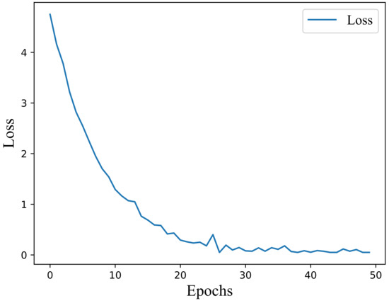
Figure 8.
Loss diagram for neural network training.
Table 3.
Complexity analysis of neural networks.
5. Analysis of Experimental Results
We proposed a technique for localization of UAV sound sources under low signal-to-noise ratio conditions in the previous section, and in this section, we verify the feasibility of the proposed method in this paper through simulation experiments and real-world experiments.
5.1. Simulation Experiment Analysis
5.1.1. DOA Algorithm Performance Comparison
DOA is the first step in localization. In this section, the DOA simulation is performed first using the test set audio generated in Chapter III to analyze the performance of each DOA algorithm in different scenarios. In order to avoid the influence of different audio samples of the sound source on DOA, except for the ordinary GCC-PHAT algorithm and the GCC-PCNN-PHAT algorithm proposed in this paper, the sound sources of the other algorithms used in the simulation for DOA are the audio of the test set.
- Simulation of each DOA estimation algorithm for microphone arrays shooting in different directions
This simulation is based on a configuration that uses audio lengths ranging from about 14,000–16,000 samples. The UAV source is 10 m away from the midpoint of the array, and the array consists of two microphones spaced 0.5 m apart. The FFT points are 1024, and the noise is additive Gaussian white noise with a signal-to-noise ratio of 10 dB. The evaluation metrics are planned to be the Root Mean Square Error (RMSE), since there is always a certain amount of error in the estimation versus the true value.
The three DOA estimation algorithms are compared in Figure 9. The GCC-PHAT algorithm refers to the use of generalized correlation to directly estimate the delay and thus obtain the DOA; the GCC-PCNN-PHAT algorithm is the algorithm proposed in this paper; the MUSIC algorithm is the narrowband MUSIC-DOA for all frequency points (including all FFT points) and then fuses all the results to obtain the final DOA. The RMSE is used for the evaluation metrics and here the observation is the angle degrees. The corresponding RMSE on each angle in Figure 9 is obtained after four hundred (400 test set UAV audio files) DOA estimations.
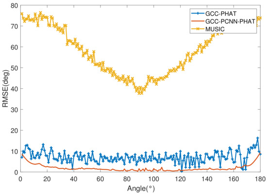
Figure 9.
RMSE for each DOA estimation algorithm for sound sources at different orientations.
The general trend of the four curves in the figure is consistent with “higher on both sides, lower in the middle”, which means that no matter which algorithm is used, the closer the source is to the 90° direction that is perpendicular to the center of the array, the lower the RMSE of the DOA estimate of the array, and the source is easily and correctly oriented. Our proposed GCC-PCNN-PHAT algorithm based on convolutional neural network performs well in terms of the RMSE of DOA estimation, and the overall RMSE is lower than that of GCC-PHAT. It breaks through the resolution limitation with the acoustic signal sampling rate already fixed, and the RMSE is lower than 1 in the 88° direction. This simulation shows that in the scenario of DOA estimation for UAV sound sources, the algorithm of estimating the time delay and then finding the DOA using GCC-PHAT is slightly better than the MUSIC-NAS algorithm, whereas the GCC-PCNN-PHAT with neural network enhancement has a much better performance on the basis of GCC-PHAT.
- Simulation of each DOA estimation algorithm with different signal-to-noise ratios
This simulation is based on the configurations −10, −6, −2, 2, 6 and 10 dB SNR. According to the results in Figure 9, we choose a fixed angle of 88° near the 90° direction as the angle at which the source is injected into the array, and the rest of the configurations are consistent with those in Section 5.1.1. Figure 10 demonstrates the RMSE comparison of each DOA estimation algorithm for different SNRs.
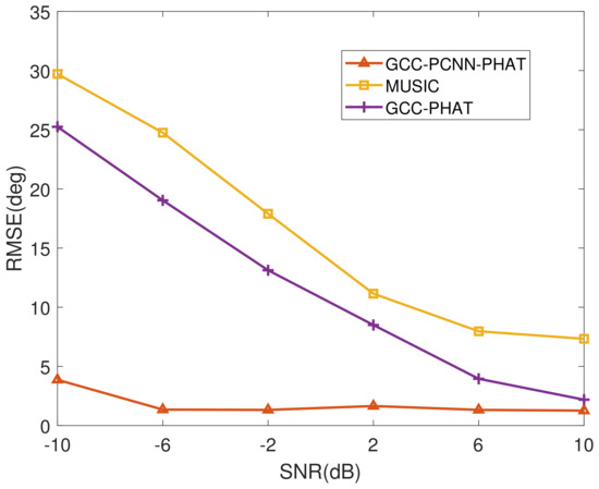
Figure 10.
RMSE of various DOA estimation algorithms with different SNR.
From Figure 10, it can be found that the RMSE of both GCC-PHAT and MUSIC-NAS algorithms increase as the SNR decreases, while the GCC-PCNN-PHAT algorithm has excellent noise immunity. This is mainly due to the fact that its model is trained with microphone signals whose SNR is randomly valued between -10 and 10 dB, so it can flexibly adjust its selection of microphone signal features under different SNRs through the nonlinear mapping of the neural network, and thus stabilize the DOA estimation at a relatively accurate level.
- Effect of audio length on noise immunity of DOA estimation algorithm
The audio length is directly related to the amount of computation required. According to Equation (22), a minimum of 49 points is theoretically sufficient to estimate the delay and thus the DOA when the array microphone spacing and sampling rate are fixed at 0.5 m and 16 kHz. Next, a simulation is performed to verify that the simulation is based on a configuration that is identical to the one in the previous section except for the change in audio length. The specific way to change the audio length is to intercept the first L samples, L = 5000, 500, 50, on each sample of length 16,000 or so. Figure 11 shows the RMSE performance of DOA estimation for different lengths of audio with different SNRs.
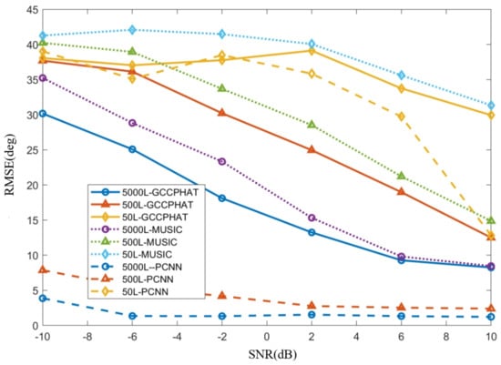
Figure 11.
RMSE for DOA estimation for different lengths of audio at different SNR.
We label the proposed algorithms as PCNN because of the length of the figure, 5000 L means the audio length is 5000 in the figure example, and so on. From Figure 11, all three algorithms are consistent with the performance of “the shorter the audio length, the worse the noise immunity”. We know that when the number of FFT points is fixed and larger than the signal length, the longer the signal length corresponds to the higher spectral resolution. As can be seen from the comparison in Figure 12 and Figure 13, when the length of the audio is shortened to 500 dots, there are also a very large number of spikes in directions other than the correct DOA, all of which are noise.
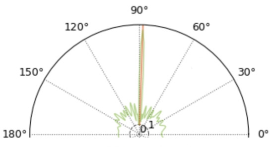
Figure 12.
Spatial spectrum of a microphone array with an audio length of 16,000.
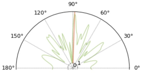
Figure 13.
Spatial spectrum of a microphone array with an audio length of 500.
The PCNN algorithm, while outperforming the other two algorithms in terms of metrics at a length of 50, also loses the ability to reliably DOA estimate. The analysis here suggests that the reliability of PCNN is very much dependent on the feature matrix shown in Equation (25). And, is also generated on the basis of the cross-correlation computation, so essentially the reason for the failure of PCNN at low signal-to-noise ratios is the same as that of the GCC-PHAT algorithm, which belongs to incorrect cross-correlation results.
5.1.2. Localization Simulation
After the simulation analysis in the previous subsection, it is generally found that the GCC-PHAT delay estimation algorithm and our proposed PCNN delay estimation algorithm perform better in terms of DOA, so these two algorithms are used for the first step of DOA in the simulation in this subsection. The localization system is shown in Figure 2, and the spacing L between the two subarrays is set to 5 m.
We first artificially set up a 3D curve as the simulated UAV trajectory and take 90 points uniformly on this curve, each point as the coordinates of the sound source at different moments, and Mic1 in Figure 2 as the origin of the coordinate system. The drone audio is used as the sound source, which is about 20 m away from the origin at its farthest point. The street sound is mixed into the signal received by the simulated microphone as noise, and the signal-to-noise ratio is set to 0 dB. Then, the localization simulation is carried out using the GCC-PHAT algorithm and algorithms, respectively. The simulation results are shown in Figure 14.
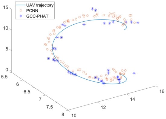
Figure 14.
Simulation results of microphone array localization of UAV sound source at 0 dB SNR.
As can be seen in Figure 14, the trajectories formed by both algorithms have some errors with the simulated real trajectories, within 0.5 m. The localization algorithm using the GCC-PHAT delay estimation DOA is obviously limited by the sampling rate accuracy: when the z-coordinate of the sound source is low, different points on the trajectory of a section of the sound source are more likely to be localized to the same point, which creates the same effect as the “clustering” in the figure. When the z-coordinate of the sound source is high, it is more scattered. The PCNN algorithm based on the deep convolutional neural network has a more uniform distribution of coordinates, and the points are more like a continuous curve than the points localized by the GCC-PHAT algorithm. Figure 15 quantitatively analyzes the errors of the two algorithms. It can be seen that the GCC-PHAT algorithm has large ups and downs in all three directions, while the PCNN algorithm has a smoother error curve. In the y-direction, the PCNN algorithm is significantly better than the GCC-PHAT algorithm in terms of localization accuracy. In the x-direction, the mean error of the PCNN algorithm is slightly smaller than that of the GCC-PHAT algorithm. In the z-direction, the PCNN algorithm’s mean error is similar to that of the GCC-PHAT algorithm, but it is more stable than the GCC-PHAT algorithm.

Figure 15.
Quantitative analysis of localization error at 0 dB SNR.
Based on the parameter settings of the previous simulation, we adjusted the SNR to −10 dB and kept the rest of the parameters unchanged, and the simulation results are shown in Figure 16. We found that when the height of the source exceeded 5 m, the GCC-PHAT algorithm could not estimate the pitch angle of the source properly under the SNR conditions, which led to an error in the second localization step (the pitch angle was estimated to be 0°). On the other hand, the PCNN algorithm proposed in this paper can form a coherent trajectory after the height of the sound source exceeds 5 m, and the form of the trajectory matches the simulated real trajectory, although the estimation error is larger than that in Figure 14, which is from 0.5 m to 1 m.
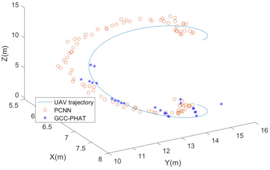
Figure 16.
Simulation results of microphone array localization of UAV sound source at −10 dB SNR.
For the purpose of error comparison, here both algorithms keep the results of the first 50 simulation points. From Figure 17, the PCNN algorithm has a significantly smaller error in the x-direction than the GCC-PHAT algorithm, while the mean error in the y-direction is not significantly smaller than the GCC-PHAT algorithm as in Figure 15, but it is still slightly smaller. In the z-direction, the mean errors of the two algorithms are still similar, but the PCNN algorithm error curve is still more stable than the GCC-PHAT algorithm. In conclusion, compared with the GCC-PHAT algorithm, the PCNN algorithm can make the microphone array maintain better accuracy in UAV sound source localization with a lower signal-to-noise ratio.
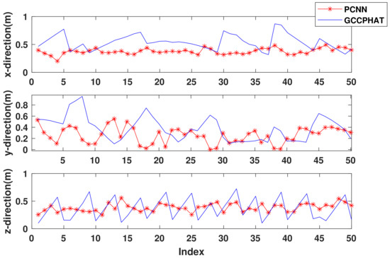
Figure 17.
Quantitative analysis of localization error at −10 dB SNR.
In order to be able to quantitatively analyze the effectiveness of the algorithms proposed in this paper, we performed t-tests as well as the calculation of the variance and the mean of the three-axis localization errors for Figure 15 and Figure 17. The results are shown in Table 4. As can be seen from the table, the error of our proposed PCNN algorithm is smaller than that of the GCC-PTAH method in both the standard deviation and the mean parts, either with a SNR of 0 dB or −10 dB. In order to assess the statistics of the difference between the means of the variables from the two samples, we introduce the t-test. Generally, we consider that a p-val less than 0.05 or less indicates a significant difference between the two sample variables. As can be seen from the table, the p-val in the x-axis direction and y-axis direction are much less than 0.05 in the environments with SNR of 0 dB and −10 dB, indicating the stability of our proposed PCNN algorithm. The variability in the z-axis is not large, and we analyze that the possible reason is related to the spatial arrangement of the microphone arrays in terms of distribution location, which will be the focus of our research in a subsequent work.
Table 4.
Quantitative analysis of the standard deviation, average value, and t-test of the three-axis error at signal-to-noise ratios of 0 dB and −10 dB.
5.2. Practical Experimental Analysis
In this section, we build a physical UAV identification and localization system to physically verify the techniques proposed in Section 3. The building process of the physical system is firstly introduced, including the selection of hardware and the way of combining each module. Then, the field environment of the experiment is introduced. Finally, the verification experiment of UAV localization is carried out.
5.2.1. Experimental Environment and System Construction
According to the characteristic that UAV sound source localization belongs to free-field measurement, the MP-40 electret microphone from Beijing Acoustic Science Measurement Company was firstly selected. After selecting the microphone, an appropriate signal conditioner was selected based on a set of parameters of this microphone. The microphone array is physically shown in Figure 18, and its bracket is self-made using aluminum alloy material according to the layout in Figure 2, with adjustable spacing between each microphone. The target UAV was selected as DJI Mini2.
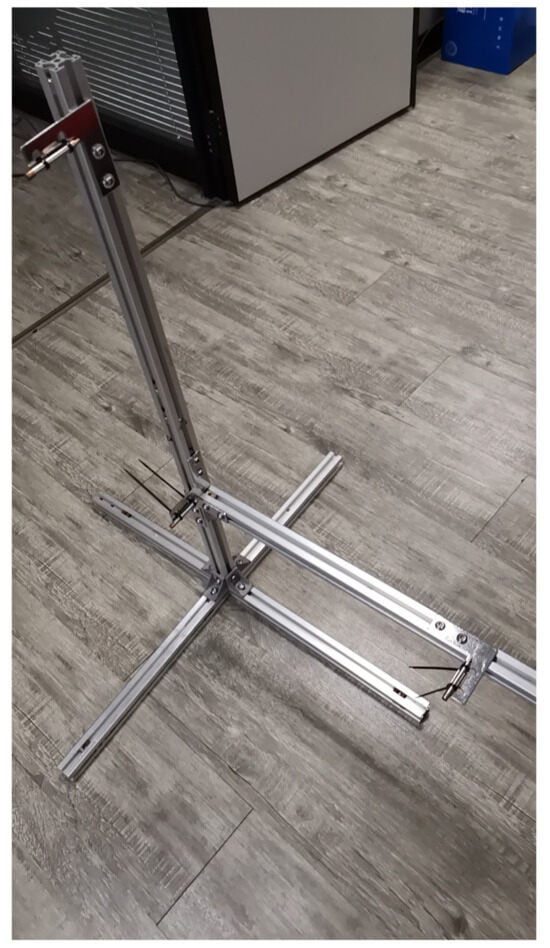
Figure 18.
Microphone array physical.
The experimental environment is shown in Figure 19, in which the devices have been connected and debugged. The experimental location is the terrace between Building A and Building B of the Innovation Building of Xiamen Software Park Phase I, adjacent to the road. The time of the experiment was around 17:20 on Friday, when the traffic was dense at the end of the day and the construction was in progress on the opposite side of the road, so the experimental environment was typical of urban noise.
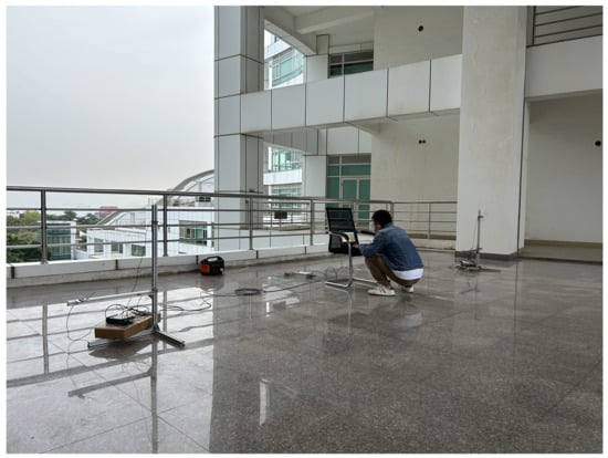
Figure 19.
Field validation environment.
5.2.2. Localization Experiments and Analysis
Since there is still a relative lack of technical means to accurately obtain the three-dimensional spatial coordinates of the UAV, the validation purpose of the experiments in this subsection is to ensure that the trajectory of the UAV determined by the microphone array is roughly in line with its real trajectory. In addition, the GPS positioning system that comes with the UAV is unable to set an obvious trajectory in a small area, so the real trajectory of the experiment is recorded by means of cell phone video. In order to facilitate the trajectory verification, the trajectory should not be designed to be very complicated. In this experiment, the trajectory is set as follows: firstly, the UAV hovers at a position in the middle of the two subarrays, which is close to the straight line where the two subarrays are located; then, it keeps the X coordinate value unchanged, flies away from the array (the Y coordinate value becomes bigger), then rises (the Z coordinate value becomes bigger), then flies back for a short time (the Y coordinate value becomes smaller but does not return to the starting position), and then lands.
Figure 20 demonstrates the exact process of capturing drone noise in the experiment. In addition to the drone noise, we also captured the ambient noise when no drone was flying. Assuming that the ambient noise at the experimental location is smooth, the actual signal-to-noise ratio when capturing the drone acoustic signal can be calculated using the captured pure ambient noise signal, which is calculated to be about 2.3 dB. The final drone acoustic signal is captured for about 50 s. In MATLAB, the signal is segmented by one frame per second, and each frame is localized once. The localization result is shown in Figure 21.
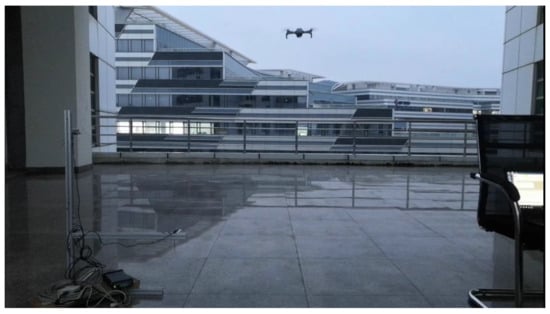
Figure 20.
Experimental procedure.
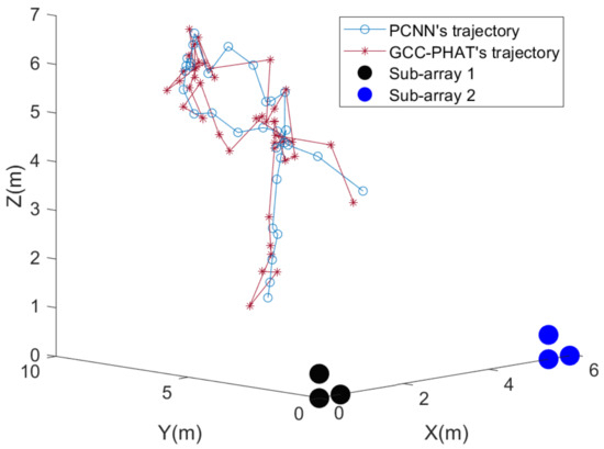
Figure 21.
Results of physical microphone array localization of UAV at 2.3 dB SNR.
As can be seen from Figure 21, at a signal-to-noise ratio of about 2.3 dB, both methods can roughly localize the trajectory of the UAV and roughly match the planned one. The fluctuation of the localization coordinates of the PCNN algorithm is smaller than that of the GCC-PHAT algorithm when the sound source is farther away from the microphone array. Since the X coordinate value of the UAV set trajectory is unchanged, Figure 22 can show the difference between the two methods in more detail in the Y-Z plane. It can be seen that the overall fluctuations of the folds formed by the coordinates estimated by the PCNN algorithm are smaller compared to the GCC-PHAT algorithm.
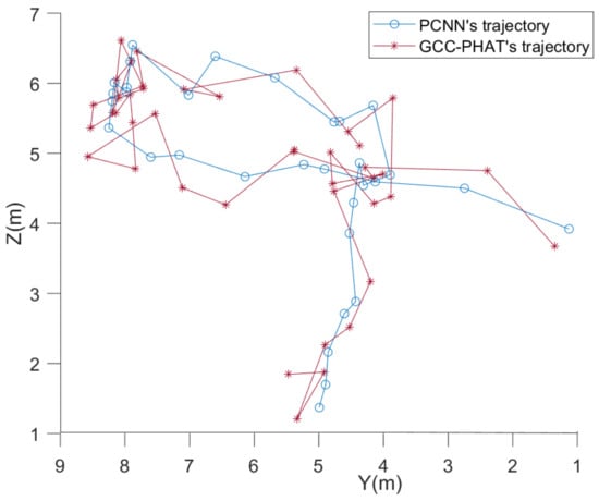
Figure 22.
Two-dimensional display of the results of physical microphone array localization of UAVs at 2.3 dB signal-to-noise ratio.
Since the signal-to-noise ratio of the field environment is difficult to control artificially, we utilize the acquired UAV acoustic signal and the pure environmental noise signal. The pure noise signal is amplified in MATLAB and mixed into the UAV noise signal to achieve a signal-to-noise ratio of −8 dB. The same 50 s UAV acoustic signal is localized again, and the results are shown in Figure 23.
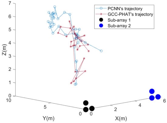
Figure 23.
Results of physical microphone array localization of UAV at −8 dB SNR.
From Figure 23, when the SNR drops to −8 dB, the straight line distance between the UAV and the microphone array is more than 15 m, and the GCC-PHAT method can no longer be used to locate the UAV. At this low SNR, the PCNN method can still locate the coordinates of the UAV well within 20 m. From Figure 24, which shows the trajectory of the UAV in the Y-Z plane, it is clear that the PCNN algorithm is able to estimate the coordinates of the points with the Y coordinate value greater than 6 at this low S/N. The GCC-PHAT algorithm is not able to locate the UAV with the GCC-PHAT algorithm at this time. In contrast, the GCC-PHAT algorithm estimates points with Y-coordinate values as high as 6, and the Y-coordinate values fluctuate significantly more than the PCNN algorithm during the descent of the UAV.
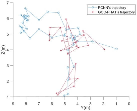
Figure 24.
Two-dimensional display of the results of physical microphone array localization of UAVs at −8 dB signal-to-noise ratio.
6. Conclusions
In this paper, we carry out research on UAV localization techniques based on acoustic means, focusing on UAV localization in low signal-to-noise ratio environments. We propose a DOA algorithm based on normalized mean pseudo-spectral MUSIC and a DOA estimation algorithm based on a time delay estimation neural network to improve the accuracy of UAV sound source localization under low signal-to-noise ratio conditions. In our experiments, we build a microphone array physical system by ourselves and rely on this system to verify the UAV localization technique proposed in this paper. In our future work, we will consider adding generative adversarial networks to our task as a way to simulate different frequencies and amplitudes of UAV noise and solve the problem of fewer samples in UAV localization.
Author Contributions
S.W. developed the method and wrote the manuscript; Y.Z., K.Y. and H.C.designed and carried out the data analysis, X.Z. and H.S. reviewed and edited themanuscript. All authors have read and agreed to the published version of the manuscript.
Funding
This work was supported by the National Natural Science Foundation of China under Grant 62271426 and Natural Resources Science and Technology Innovation Project of Fujian Province (KY-080000-04-2022-025).
Data Availability Statement
The data presented in this study are available on request from theauthor. The data are not publicly available due to privacy restrictions.
Conflicts of Interest
Author Xuebo Zhang was employed by the Whale Wave Technology Inc. The remaining authors declare that the research was conducted in the absence of any commercial or financial relationships that could be construed as a potential conflict of interest.
References
- Hilal, A.A.; Mismar, T. Drone Positioning System Based on Sound Signals Detection for Tracking and Photography. In Proceedings of the 2020 11th IEEE Annual Information Technology, Electronics and Mobile Communication Conference (IEMCON), Vancouver, BC, Canada, 4–7 November 2020; pp. 8–11. [Google Scholar]
- Yamada, T.; Itoyama, K.; Nishida, K.; Nakadai, K. Outdoor evaluation of sound source localization for drone groups using microphone arrays. In Proceedings of the 2022 IEEE/RSJ International Conference on Intelligent Robots and Systems (IROS), Kyoto, Japan, 23–27 October 2022; pp. 9296–9301. [Google Scholar]
- Zhang, H.; Li, T.; Li, Y.; Li, J.; Dobre, O.A.; Wen, Z. RF-Based Drone Classification Under Complex Electromagnetic Environments Using Deep Learning. IEEE Sens. J. 2023, 23, 6099–6108. [Google Scholar] [CrossRef]
- Coluccia, A.; Fascista, A.; Schumann, A.; Sommer, L.; Dimou, A.; Zarpalas, D.; Akyon, F.C.; Eryuksel, O.; Ozfuttu, K.A.; Altinuc, S.O.; et al. Drone-vs-Bird Detection Challenge at IEEE AVSS2021. In Proceedings of the 2021 17th IEEE International Conference on Advanced Video and Signal Based Surveillance (AVSS), Washington, DC, USA, 16–19 November 2021; pp. 1–8. [Google Scholar]
- Chiper, F.-L.; Martian, A.; Vladeanu, C.; Marghescu, I.; Craciunescu, R.; Fratu, O. Drone Detection and Defense Systems: Survey and a Software-Defined Radio-Based Solution. Sensors 2022, 22, 1453. [Google Scholar] [CrossRef] [PubMed]
- Ezuma, M.; Erden, F.; Anjinappa, C.K.; Ozdemir, O.; Guvenc, I. Micro-UAV Detection and Classification from RF Fingerprints Using Machine Learning Techniques. In Proceedings of the 2019 IEEE Aerospace Conference, Big Sky, MT, USA, 2–9 March 2019; pp. 1–13. [Google Scholar]
- Medaiyese, O.O.; Syed, A.; Lauf, A.P. Machine Learning Framework for RF-Based Drone Detection and Identification System. In Proceedings of the 2021 2nd International Conference On Smart Cities, Automation & Intelligent Computing Systems (ICON-SONICS), Tangerang, Indonesia, 12–13 October 2021; pp. 58–64. [Google Scholar]
- Semkin, V.; Yin, M.; Hu, Y.; Mezzavilla, M.; Rangan, S. Drone Detection and Classification Based on Radar Cross Section Signatures. In Proceedings of the 2020 International Symposium on Antennas and Propagation (ISAP), Osaka, Japan, 25–28 January 2021; pp. 223–224. [Google Scholar]
- Ezuma, M.; Anjinappa, C.K.; Funderburk, M.; Guvenc, I. Radar Cross Section Based Statistical Recognition of UAVs at Microwave Frequencies. IEEE Trans. Aerosp. Electron. Syst. 2022, 58, 27–46. [Google Scholar] [CrossRef]
- Nalamati, M.; Kapoor, A.; Saqib, M.; Sharma, N.; Blumenstein, M. Drone Detection in Long-Range Surveillance Videos. In Proceedings of the 2019 16th IEEE International Conference on Advanced Video and Signal Based Surveillance (AVSS), Taipei, Taiwan, 18–21 September 2019; pp. 1–6. [Google Scholar]
- Shi, X.; Yang, C.; Xie, W.; Liang, C.; Shi, Z.; Chen, J. Anti-Drone System with Multiple Surveillance Technologies: Architecture, Implementation, and Challenges. IEEE Commun. Mag. 2018, 56, 68–74. [Google Scholar] [CrossRef]
- Svanström, F.; Englund, C.; Alonso-Fernandez, F. Real-Time Drone Detection and Tracking With Visible, Thermal and Acoustic Sensors. In Proceedings of the 2020 25th International Conference on Pattern Recognition (ICPR), Milan, Italy, 10–15 January 2021; pp. 7265–7272. [Google Scholar]
- Ganti, S.R.; Kim, Y. Implementation of detection and tracking mechanism for small UAS. In Proceedings of the 2016 International Conference on Unmanned Aircraft Systems (ICUAS), Arlington, VA, USA, 7–10 June 2016; pp. 1254–1260. [Google Scholar]
- Behera, D.K.; Raj, A.B. Drone Detection and Classification using Deep Learning. In Proceedings of the 2020 4th International Conference on Intelligent Computing and Control Systems (ICICCS), Madurai, India, 13–15 May 2020; pp. 1012–1016. [Google Scholar]
- Guvenc, I.; Koohifar, F.; Singh, S.; Sichitiu, M.L.; Matolak, D. Detection, Tracking, and Interdiction for Amateur Drones. IEEE Commun. Mag. 2018, 56, 75–81. [Google Scholar] [CrossRef]
- Aydın, İ.; Kızılay, E. Development of a new light-weight convolutional neural network for acoustic-based amateur drone detection. Appl. Acoust. 2022, 193, 108773. [Google Scholar] [CrossRef]
- Chung, M.A.; Chou, H.C.; Lin, C.W. Sound localization based on acoustic source using multiple microphone array in an indoor environment. Electronics 2022, 11, 890. [Google Scholar] [CrossRef]
- Al-Emadi, S.; Al-Ali, A.; Mohammad, A.; Al-Ali, A. Audio Based Drone Detection and Identification using Deep Learning. In Proceedings of the 2019 15th International Wireless Communications & Mobile Computing Conference (IWCMC), Tangier, Morocco, 24–28 June 2019; pp. 459–464. [Google Scholar]
- Knapp, C.; Carter, G. The generalized correlation method for estimation of time delay. IEEE Trans. Acoust. Speech Signal Process. 1976, 24, 320–327. [Google Scholar] [CrossRef]
- DiBiase, J.H.; Silverman, H.F.; Brandstein, M. Robust Localization in Reverberant Rooms; Springer: Berlin/Heidelberg, Germany, 2001. [Google Scholar]
- Dmochowski, J.P.; Benesty, J.; Affes, S. Broadband Music: Opportunities and Challenges for Multiple Source Localization. In Proceedings of the 2007 IEEE Workshop on Applications of Signal Processing to Audio and Acoustics, New Paltz, NY, USA, 21–24 October 2007; pp. 18–21. [Google Scholar]
- Chakrabarty, S.; Habets, E.A.P. Broadband doa estimation using convolutional neural networks trained with noise signals. In Proceedings of the 2017 IEEE Workshop on Applications of Signal Processing to Audio and Acoustics (WASPAA), New Paltz, NY, USA, 15–18 October 2017; pp. 136–140. [Google Scholar]
- Perotin, L.; Serizel, R.; Vincent, E.; Guérin, A. CRNN-based Joint Azimuth and Elevation Localization with the Ambisonics Intensity Vector. In Proceedings of the 2018 16th International Workshop on Acoustic Signal Enhancement (IWAENC), Tokyo, Japan, 17–20 September 2018; pp. 241–245. [Google Scholar]
- Adavanne, S.; Politis, A.; Virtanen, T. Direction of Arrival Estimation for Multiple Sound Sources Using Convolutional Recurrent Neural Network. In Proceedings of the 2018 26th European Signal Processing Conference (EUSIPCO), Rome, Italy, 3–7 September 2018; pp. 1462–1466. [Google Scholar]
- Vera-Diaz, J.M.; Pizarro, D.; Macias-Guarasa, J. Towards end-to-end acoustic localization using deep learning: From audio signals to source position coordinates. Sensors 2018, 18, 3418. [Google Scholar] [CrossRef] [PubMed]
- Salvati, D.; Drioli, C.; Foresti, G.L. Time delay estimation for speaker localization using cnn-based parametrized gcc-phat features. In Proceedings of the Conference of the International Speech Communication Association, Brno, Czechia, 30 August–3 September 2021. [Google Scholar]
- Diaz-Guerra, D.; Miguel, A.; Beltran, J.R. Robust sound source tracking using srp-phat and 3d convolutional neural networks. IEEE/ACM Trans. Audio Speech Lang. Process. 2020, 29, 300–311. [Google Scholar] [CrossRef]
- Case, E.E.; Zelnio, A.M.; Rigling, B.D. Low-cost acoustic array for small uav detection and tracking. In Proceedings of the 2008 IEEE National Aerospace and Electronics Conference, Dayton, OH, USA, 16–18 July 2008; pp. 110–113. [Google Scholar]
- Yang, B.; Matson, E.T.; Smith, A.H.; Dietz, J.E.; Gallagher, J.C. Uav detection system with multiple acoustic nodes using machine learning models. In Proceedings of the 2019 Third IEEE International Conference on Robotic Computing (IRC), Naples, Italy, 25–27 February 2019. [Google Scholar]
- Shi, Z.; Chang, X.; Yang, C.; Wu, Z.; Wu, J. An acoustic-based surveillance system for amateur drones detection and localization. IEEE Trans. Veh. Technol. 2020, 69, 2731–2739. [Google Scholar] [CrossRef]
- Carter, G.C. Coherence and time delay estimation. Proc. IEEE 1987, 75, 236–255. [Google Scholar] [CrossRef]
- Schmidt, R. Multiple emitter location and signal parameter estimation. IEEE Trans. Antennas Propag. 1986, 34, 276–280. [Google Scholar] [CrossRef]
- Tao, T.; Zheng, H.; Yang, J.; Guo, Z.; Zhang, Y.; Ao, J.; Chen, Y.; Lin, W.; Tan, X. Sound Localization and Speech Enhancement Algorithm Based on Dual-Microphone. Sensors 2022, 22, 715. [Google Scholar] [CrossRef] [PubMed]
- Yousaf, J.; Zia, H.; Alhalabi, M.; Yaghi, M.; Basmaji, T.; Shehhi, E.A.; Gad, A.; Alkhedher, M.; Ghazal, M. Drone and controller detection and localization: Trends and challenges. Appl. Sci. 2022, 12, 12612. [Google Scholar] [CrossRef]
- Salvati, D.; Drioli, C.; Foresti, G.L. Incoherent Frequency Fusion for Broadband Steered Response Power Algorithms in Noisy Environments. IEEE Signal Process. Lett. 2014, 21, 581–585. [Google Scholar] [CrossRef]
- Scheibler, R.; Bezzam, E.; Dokmanić, I. Pyroomacoustics: A Python Package for Audio Room Simulation and Array Processing Algorithms. In Proceedings of the 2018 IEEE International Conference on Acoustics, Speech and Signal Processing (ICASSP), Calgary, AB, Canada, 15–20 April 2018; pp. 351–355. [Google Scholar]
Disclaimer/Publisher’s Note: The statements, opinions and data contained in all publications are solely those of the individual author(s) and contributor(s) and not of MDPI and/or the editor(s). MDPI and/or the editor(s) disclaim responsibility for any injury to people or property resulting from any ideas, methods, instructions or products referred to in the content. |
© 2024 by the authors. Licensee MDPI, Basel, Switzerland. This article is an open access article distributed under the terms and conditions of the Creative Commons Attribution (CC BY) license (https://creativecommons.org/licenses/by/4.0/).