Abstract
Forest structural parameters are crucial for assessing ecological functions and forest quality. To improve the accuracy of estimating these parameters, various approaches based on remote sensing platforms have been employed. Although remote sensing yields high prediction accuracy in uniform, even-aged, simply structured forests, it struggles in complex structures, where accurately predicting forest structural parameters remains a significant challenge. Recent advancements in unmanned aerial vehicle (UAV) photogrammetry have opened new avenues for the accurate estimation of forest structural parameters. However, many studies have relied on a limited set of remote sensing metrics, despite the fact that selecting appropriate metrics as powerful explanatory variables and applying diverse models are essential for achieving high estimation accuracy. In this study, high-resolution RGB imagery from DJI Matrice 300 real-time kinematics was utilized to estimate forest structural parameters in a mixed conifer–broadleaf forest at the University of Tokyo Hokkaido Forest (Hokkaido, Japan). Structural and textual metrics were extracted from canopy height models, and spectral metrics were extracted from orthomosaics. Using random forest and multiple linear regression models, we achieved relatively high estimation accuracy for dominant tree height, mean tree diameter at breast height, basal area, mean stand volume, stem density, and broadleaf ratio. Including a large number of explanatory variables proved advantageous in this complex forest, as its structure is influenced by numerous factors. Our results will aid foresters in predicting forest structural parameters using UAV photogrammetry, thereby contributing to sustainable forest management.
1. Introduction
Forest structure encompasses the vertical, horizontal, and unified patterns of trees, branches, understory, and canopy gaps, along with nonliving elements such as soils and hydrology [1,2,3]. It profoundly influences ecosystem functions such as wood production, erosion control, and biodiversity [4,5,6]. Recognizing its significance, foresters integrate forest structure considerations into decision-making processes. Forest structural parameters enable specific quantitative assessments of different aspects of the forest structure. Quantitative assessments of forest structure are important for forest management at various scales [7]. Remote sensing technology offers an alternative, providing multi-dimensional information at regional and landscape levels [8]. It facilitates the accurate assessment of structural parameters such as tree height (H) and diameter at breast height (DBH), which are crucial for estimating basal area (BA), volume (V), and carbon stock (CST) [9].
Assessments of forest structural parameters [10,11] involve various terminologies, such as stand parameters [12,13], forest structural attributes [11,14,15,16,17], forest biophysical properties [18,19,20], and tree attributes [7,21]. Previous studies have explored diverse forest structural parameters, including stand top height, mean H, max H, Lorey’s mean height (HL), stand mean DBH, number of trees, stem density (Sden), BA, stand V, and aboveground biomass (AGB), canopy cover (CC), crown area (CA), crown width, crown length, and crown volume [7,11,12,14,18,19,20,22,23,24]. In our study, we considered Hd, DBH, BA, V, CST, Sden, and the broadleaf ratio (BLr) as forest structural parameters. Field estimation of forest structural parameters is time-consuming, labor intensive, and expensive [14,25]. Although satellite images are commonly used for estimating forest structural parameters due to their widespread availability, they often suffer from low resolution and cloud occlusion issues. Manned airborne light detection and ranging (LiDAR) technology provides highly accurate information, but its high cost limits its usage [25]. Unmanned aerial vehicles (UAVs) offer flexible, reliable, and repeatable measurements through different sensors mounted on the UAV platform, including RGB, multispectral, hyperspectral, and LiDAR sensors [14]. In our study, we utilized UAV-mounted RGB sensors.
In remote sensing studies, variables used to predict forest structural parameters are height-related metrics (maximum, minimum, mean, percentile height, standard deviation, covariance, kurtosis, and skewness) and canopy attributes (canopy gap, canopy density, CC, canopy area, crown diameter, crown height, canopy V, and canopy profile metrics) [22,26,27,28,29,30]. Previous studies have estimated forest structural parameters using area-based approaches (plot, stand, or landscape level) [18,19,31], an individual-based approach [7,10,13,15,20,21], or both [14,17]. In this study, forest structural parameters were estimated using an area-based approach suitable for explaining forest complexity and spatial distribution patterns [32,33].
In remote sensing, feature selection and model construction are crucial. Previously, structural, textural, and spectral metrics were derived from canopy height models (CHMs), digital surface models (DSMs), orthomosaics, and satellite images [34,35,36,37,38,39]. The models used in previous studies included simple linear regression, partial least squares regression, generalized linear mixed model (GLMM), multiple linear regression (MLR), classification and regression tree (CART) analysis, and machine learning models such as random forest (RF), support vector machine (SVM), as well as deep learning models. Model accuracy varies depending on factors such as the study area, stand type, and environmental conditions. RF models often yield the highest estimation accuracy for forest structural predictions [29,34]. Thus, in this study, RF was used together with MLR to estimate forest structural parameters, as these models select more variables, leading to more accurate predictions.
Estimation accuracy of forest structural parameters and classification accuracy of land use significantly improved with high-resolution images [29,31,37,38,40,41]. Remote sensing structural metrics provided comparatively higher estimation accuracy [34,42]. Previous studies achieved higher estimation accuracy in complex mixed conifer–broadleaf forest for Hd (R2 = 0.82, RMSE = 1.78), DBH (R2 = 0.64, RMSE = 3.92), BA (R2 = 0.74, RMSE = 5.42), V (R2 = 0.84 and RMSE = 39.8), and CST (R2 = 0.82, RMSE = 14.3) [34] using RGB imagery with structural metrics including a few spectral metrics, while accuracy was low for Sden (R2 = 0.37, RMSE = 78) [27]. Ozdemir and Karnieli [26] obtained comparable accuracies for Sden (R2 = 0.38, RMSE = 109.56), BA (R2 = 0.54, RMSE = 1.79), and V (R2 = 0.42, RMSE = 27.18) using textural metrics. In complex mixed conifer–broadleaf forests, prediction accuracy of forest structural parameters improved when spectral and textural metrics were included alongside structural metrics [26,39]. Relatively higher estimation accuracy was obtained using airborne LiDAR point clouds for Hd (R2 = 0.87, RMSE = 1.5), DBH (R2 = 0.61, RMSE = 3.75), BA (R2 = 0.81, RMSE = 4.58), V (R2 = 0.80, RMSE = 55.04), and CST (R2 = 0.78, RMSE = 22.68) [22,29,31].
Forest structural parameter prediction is reliable and accurate for even-aged, simply structured forests and mono plantations. However, structurally complex, mixed forests often present uncertainties. Thus, for these forests, extracting suitable remote sensing metrics, selecting reliable models, and utilizing high-resolution images are crucial for estimation accuracy. However, while forest structural parameter prediction typically relies on remote sensing structural variables, textural and spectral variables have rarely been used [26,43]. Variable selection plays a pivotal role in predicting forest structure, encompassing horizontal, vertical, and three-dimensional aspects. Failure to incorporate spectral and textual variables results in less accurate estimations, especially for complex forests. UAV ‘Structure from Motion’ (SfM) digital aerial photogrammetry with RGB sensors often yields prediction accuracy comparable to LiDAR-based estimations, even with remaining uncertainties [29].
This study provides the significance of remote sensing technology in assessing forest structural parameters, emphasizing the importance of accurate predictions for effective forest management. Various methodologies and models are explored, focusing on the integration of structural, textural, and spectral metrics for improved estimation accuracy. For this, UAV-derived RGB imagery was employed to estimate plot-level forest structural parameters, including Hd, DBH, BA, V, CST, Sden, and BLr, using structural, textural, and spectral metrics. This study aimed to select suitable UAV metrics for accurate prediction of forest structural parameters and evaluate the accuracy of the different regression models.
2. Materials and Methods
2.1. Study Site
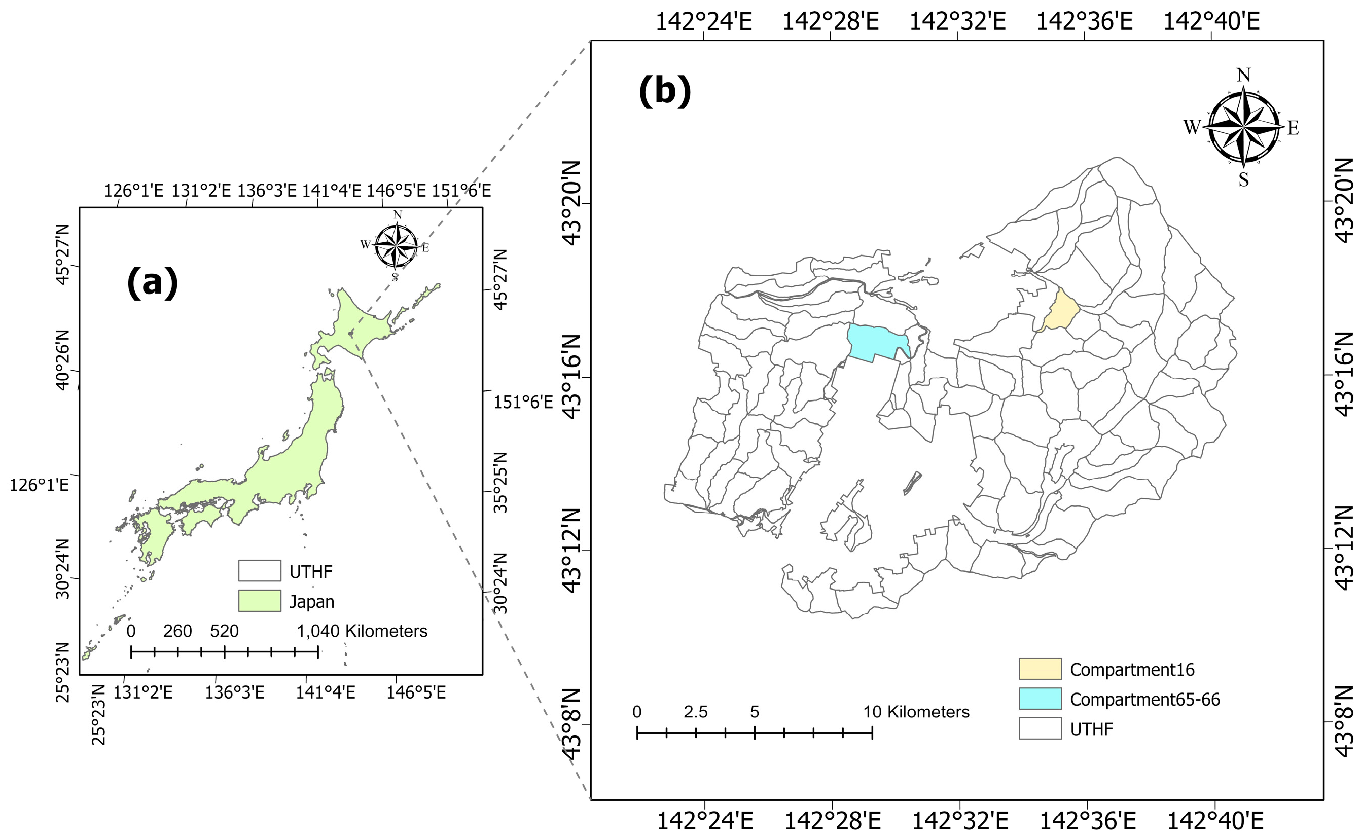
This study was conducted at the University of Tokyo Hokkaido Forest (UTHF) (43°10–20′N, 142°18–40′E, 190–1459 m asl) in Furano City, central Hokkaido Island, northern Japan (Figure 1). The UTHF is a hemiboreal, unevenly aged, complex, mixed conifer–broadleaf forest located in the transition zone between cool temperate deciduous forests and hemiboreal coniferous forests. Covering a total area of 22,717 ha, the forest features dominant conifer species such as Abies sachalinensis (Todo fir), Picea jezoensis (Jezo spruce), and P. glehnii (red spruce), alongside predominant broadleaf species such as Betula maximowicziana (birch), Quercus crispula (oak), Acer pictum var. mono (maple), Fraxinus mandshurica (Manchurian ash), Kalopanax septemlobus (castor aralia), Taxus cuspidata, and Tilia japonica (linden). Additionally, two dwarf bamboo species, Sasa senanensis and S. kurilensis, have spread over the forest floor. The arboretum experienced mean annual temperature of 6.4 °C and annual precipitation of 1297 mm (230 m asl) during 2001–2008. Snow typically covers the forest floor from late November to early April, reaching approximately 1 m in depth [34,44,45,46]. For this study, forest compartments 16 (com16) and 65-66 (com65-66) were selected as the study area (Figure 1).

Figure 1.
Map represents the study area: (a) The UTHF in Japan; (b) comp16 and comp65-66 in the UTHF.
2.2. Collection of Field Data
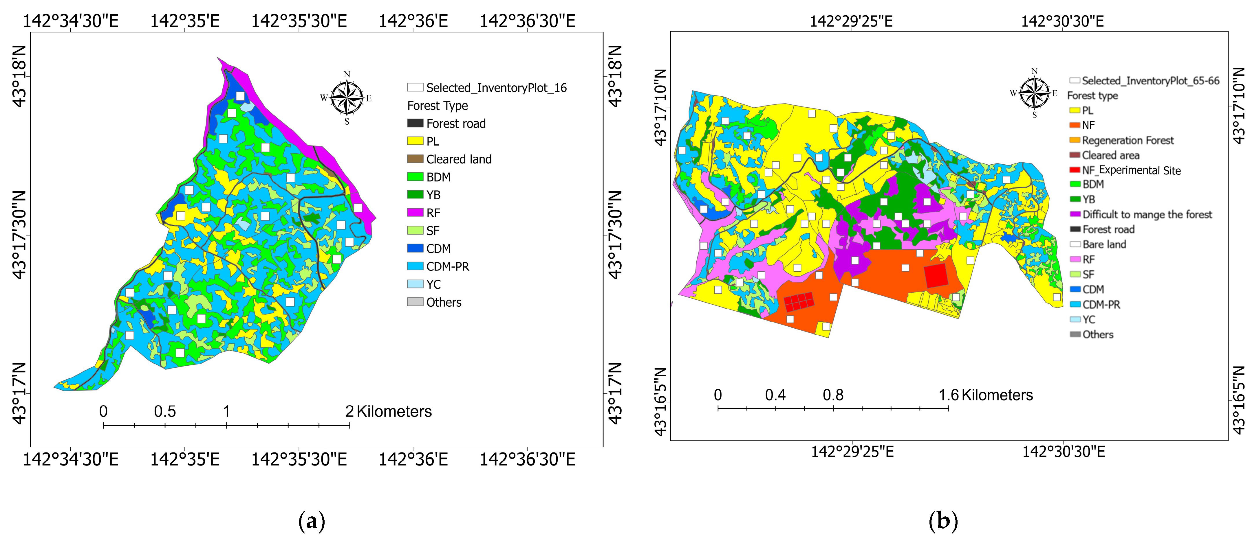
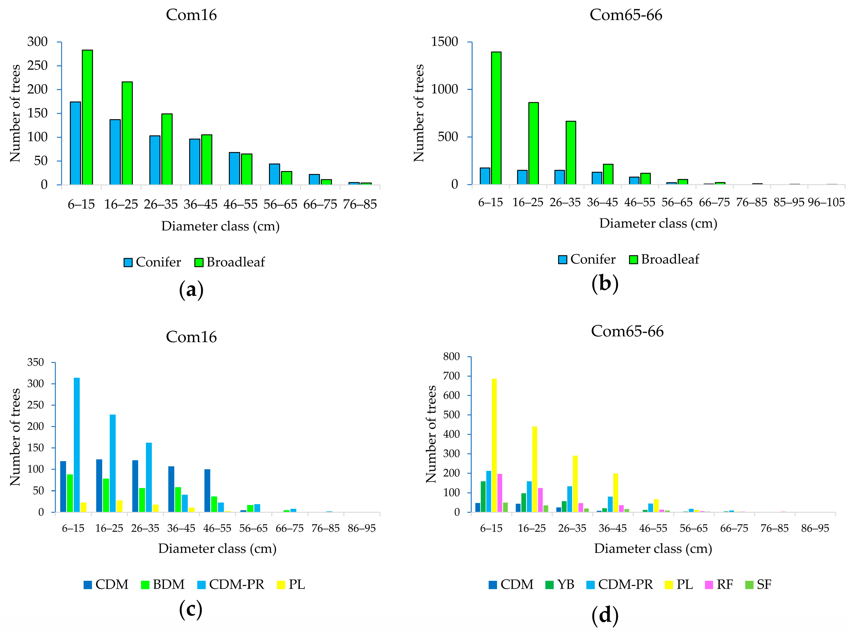
Field data were collected from 50 m × 50 m inventory plots in com16 (158 ha) and com65-66 (301 ha) (Figure 2). Rectangular plots were excluded during plot selection to maintain analysis consistency across the study area, resulting in the initial selection of 18 plots in comp16 and 51 plots in com65-66. Plot numbers varied according to the compartment size. One plot from com16 and eight plots from com65-66 were omitted based on the visual assessment of orthomosaics and the CHM to avoid edge effects and unclear or blurred portions in processed images. According to UTHF management information, com65-66, especially its southern site (Figure 2b), sustained heavier damage from a wind storm in 1981 than com16. Plantations (PL) in com65-66 are predominantly A. sachalinensis and P. glehnii planted in 1985–1986 (see the diameter class distribution in Figure A1). The field survey, conducted as an inventory plot survey measuring DBH ≥ 5 cm and a survey for Hd measurement, took place from December 2022 to March 2023. The Hd survey in April 2023 measured spatial location, Hd, and DBH (1.3 m above ground) of dominant trees. Winter measurements were taken when coniferous tree treetops were visible due to deciduous tree leaf fall, enhancing accuracy. In the inventory plots, a ratio of 80% conifer and 20% broadleaf was set for higher accuracy, with only conifer or broadleaf trees selected in the absence of the other. Eight trees with DBH ≥ 20 cm were selected from each plot based on the inventory plot data and measured using a Vertex III hypsometer with a transponder (Haglöf Sweden AB, Långsele, Sweden) to determine the Hd [34]. Two tree diameters were measured perpendicularly using tree caliber, with a lower value taken as DBH. Tree spatial locations were identified using a real-time kinematic (RTK) global navigation satellite system (GNSS) rover with a DG-PRO1RWS GNSS receiver (BizStation Corp., Matsumoto City, Japan). BA was computed based on the DBH, and tree V was estimated using a species-specific V table provided by UTHF. CST was calculated using the following allometric Equation (1):
where CST is the carbon stock in living biomass in a plot (MgC ha−1); V is the merchantable volume (m3); it is a stem volume estimated for each tree species based on the yield table developed for a given region, site class, and stand age provided by the UTHF; D is the wood density (t–d.m. m−3); BEF is the biomass expansion factor for the conversion of merchantable volume; R is the root–to–shoot ratio; CF is the carbon fraction of dry matter (MgC t–d.m.−1); and j is the tree species [47]. The summary statistics of the field data are given in Table 1. The distribution of tree diameter is given in Figure A1.

Figure 2.
The map shows the inventory plots in the classified stand type in the study compartments: (a) comp16 (n = 18); (b) comp65-66 (n = 51). In the legend, PL: plantation (yellow); BDM: broadleaf dominant mixed stand (olive green); CDM: conifer dominant mixed stand (dark blue); CDM-PR: conifer dominant mixed stand with poor regeneration (bright blue); YC: young conifer (dull blue); YB: young broadleaf (dark green); SF: sparse forest (light green); RF: reserve forest (purple); and NF: natural forest (red, which is also part of the reserve forest).

Table 1.
The results of mean value of the field forest structural parameters in com16 and com65-66.
2.3. Acquisition of UAV Imagery
Aerial imagery was collected at com16 on 28 October 2022 and at com65-66 on 26 October 2022 using the DJI Matrice 300 RTK UAV platform equipped with a DJI Zenmuse P1 RGB camera with a 35-megapixel sensor (Figure 3). The UAV employed for image collection was a light vehicle drone with a total weight of 6.3 kg, inclusive of sensors and two TB60 batteries [45].

Figure 3.
UAV flight operation in the field: (a) DJI Matrice 300 RTK UAV with a Zenmuse P1 RGB sensors at drone landing pad (orange) landing and takeoff mark; (b) TB60 batteries in the box—two batteries were used at one flight time; (c) DJI D-RTK2: a high-precision GNSS (Global Navigation Satellite System) positioning system designed for DJI UAV, providing centimeter-level accuracy in positioning for UAV; (d) ground control point (GCP): GCP for UAV is a precisely measured point by GNSS receiver, used as a reference in aerial surveys to improve the accuracy of mapping and 3D reconstruction; (e) two controllers-used to navigate the flight path and operated by two experts from the UTHF.
The flight parameters and imagery outcomes are shown in Table 2. UAV flights adhered to a preset parallel flight plan covering the study sites, maintaining a fixed altitude of 150 m above ground level at comp65-66 and 200 m at comp16. Although the Ministry of Land, Infrastructure, Transport, and Tourism of Japan imposes a flight altitude limit of ≤150 m above ground level, special permission was granted for higher flight altitudes in this study [45]. The elevated flight altitude in com16 accommodated its higher elevation, ensuring consistent image resolution. Therefore, we assumed that flight speed did not affect image quality or acquisition. Ground control point (GCP) locations were recorded using the RTK dual-frequency GNSS receiver of DG-PRO1RWS. Four checkpoints (known points in the UAV images) were used in comp65-66, with a reprojection error of 0.8 m and a sigma (deviation) of 0.3 m. No GCPs were necessary in comp16 due to the dual-frequency RTK GNSS in the Matrice 300, which provided direct georeferencing of the UAV imagery [45].

Table 2.
The UAV flight parameters setting in the comp16 and comp65-66.
2.4. Data Analysis
2.4.1. UAV Image Processing
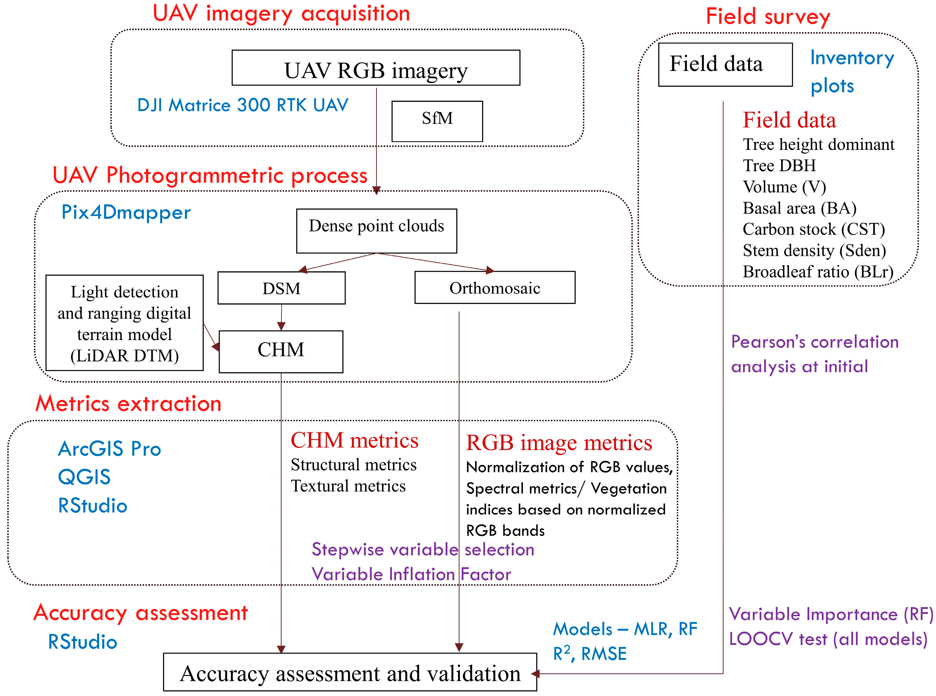
The overall workflow of the study is shown in Figure 4. Aerial images were processed using Pix4Dmapper version 4.8.0 (Lausanne, Switzerland). The software determines camera positions and orientations in three-dimensional space by analyzing feature points on different images through a SfM process to generate 3D point clouds and orthomosaic images. A total of 10,943 and 12,060 images were collected in com16 and com65-66, respectively. The photogrammetric process involved importing the UAV images, aligning images, and calibrating them to a scalable standard, followed by densification at an optimal level, mesh building with dense input, and orthomosaic generation. In both compartments, 100% calibrated images were used. The median of 4363 and 3268 matches per calibrated image was applied in com16 and com65-66, respectively. The orthomosaics had a resolution of 1.6 cm/pixel in both compartments. For comp65-66, the four aforementioned checkpoints were used to improve the accuracy of the photogrammetric products during image alignment. Georeferencing was conducted using the Japan plane rectangular CS XII (ESPG: 2454) coordinate system.

Figure 4.
The workflow of the study included field data collection; UAV photogrammetry process; canopy height model (CHM) generation; and feature extraction—CHM and orthomosaic metrics.
2.4.2. Generation of the CHMs
The LAS files of the 3D point clouds generated by Pix4Dmapper were used for generating the DSM. In ArcGIS Pro (version 2.8), the LAS data set to raster tool within the LAS conversion tool was employed to create the DSM, using the LAS point clouds as input. Parameters including the value field, interpolation type, cell assignment, void fill method, and sampling value were configured as max, binning, nearest neighbor, and five, respectively [48]. The UAV digital terrain model (DTM) exhibited low accuracy due to the occlusion effect from the top canopy. To address this, a high-precision DTM was generated by leveraging the penetration capabilities of airborne LiDAR, which offered superior vertical forest structure insights. Consequently, CHMs were generated for each UAV flight by subtracting the LiDAR DTM from the UAV DSM. The LiDAR DTM was derived using an Optech airborne laser terrain mapper (ALTM) Orion M300 sensor (Teledyne Technologies, Thousand Oaks, CA, USA) mounted on a helicopter in 2018 by the UTHF. The helicopter flew 600 m aboveground at a speed of 140.4 km h−1. The LiDAR data parameters included a course overlap of 50%, a pulse rate of 100 kHz, a scan angle of ±20°, a beam divergence of 0.16 mrad, and a point density of 11.6 points per m2 (Hokkaido Aero Asahi, Hokkaido, Japan), stored in LAS format [49]. The resulting LiDAR DTM exhibited minimum height, max height, average height, RMSE, and standard deviations of 0.02 m, 0.14 m, 0.00 m, 0.061 m, and 0.061 m, respectively. The LiDAR DTM was clipped within the forest compartment stand area to generate the CHM. The raster calculator in ArcGIS Pro was used to remove <2 m CHM to avoid ground layer interference. The resolution for CHMs, DSM, and DTM was 0.5 m/pixel.
2.4.3. Extraction of Metrics from the Generated CHM and Orthomosaics
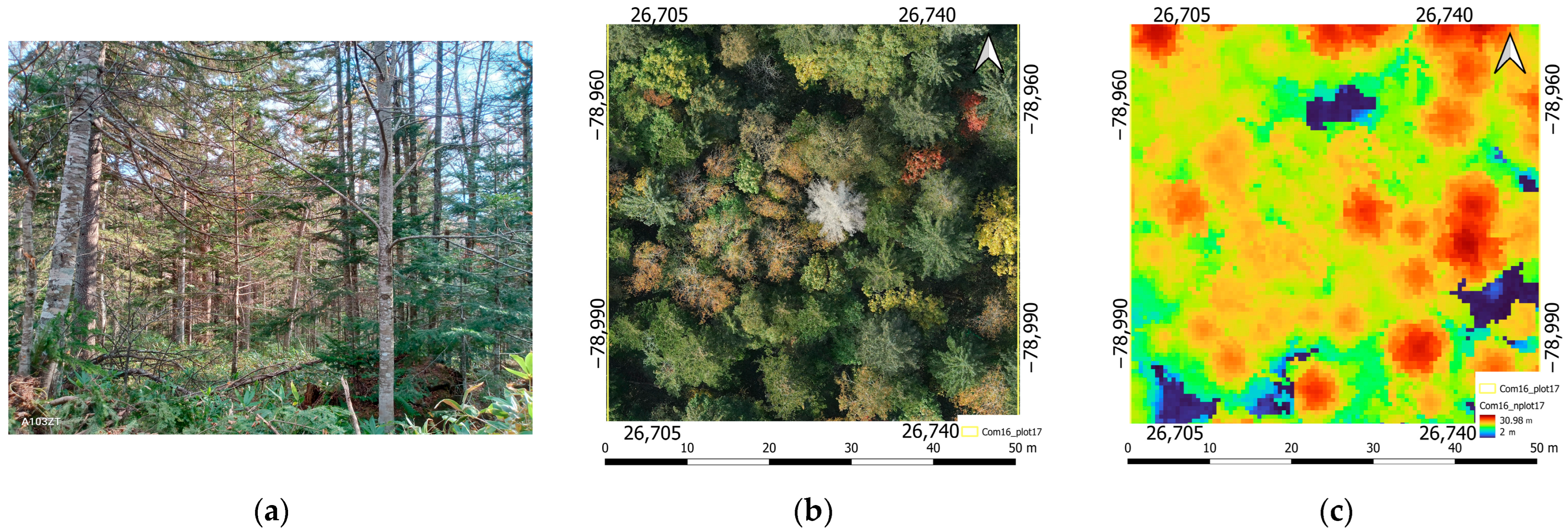
The generated CHMs and orthomosaics were used to extract structural, textural, and spectral metrics for each plot within the two forest compartments (Figure 5). The CHM specific to each plot was clipped to facilitate the extraction of its structural and textural metrics. Spectral metrics, such as vegetation indices related to RGB bands, were derived (Table 3). Image collection occurred on sunny days under clear atmospheric conditions, ensuring optimal conditions for accurate image processing using Pix4Dmapping software. However, in com65-66, unclear and blurred sections at the orthomosaic edges led to improbable height ranges in the DSM and subsequently in the CHM. Consequently, 8 plots out of 51 inventory plots with unclear, blurred, and shaded areas in their images were excluded. In comp16, one plot exhibited a significantly deviant field height from the CHM and was therefore eliminated, resulting in seventeen remaining plots. Careful consideration was given to parameter settings during image processing to minimize the need for repeated processing and ensure satisfactory 3D reconstruction [50]. Spectral metrics rely heavily on RGB bands. Spectral metrics were derived from the normalized values of the R, G, and B bands in each plot [46] due to the time difference in the orthomosaics of the two compartments. The accuracy of the analysis depends on the number of plots selected. A smaller number of plots was chosen in com16 (n =17) compared to com65-66 (n = 43) due to the selected plot size of 50 m × 50 m for analysis purposes and for the development of stand-level wall-to-wall mapping based on 50 m × 50 m grids for future studies [29].

Figure 5.
Illustration of an inventory plot (50 m × 50 m) in the field: (a) plot in the field; (b) orthomosaic of a plot; (c) CHM of a plot.
Textual metrics were computed based on field plot pixels using the gray level co-occurrence matrix (GLCM) [26], a method to measure relative pixel brightness and detect gray level differences [43,51]. Mean and maximum CHM values, along with the coefficient of variation (cv), were derived using ArcGIS Pro statistics. CD metrics were extracted using the raster package in RStudio version 4.22. Roughness and texture were obtained via the roughness algorithm of the Geospatial Data Abstraction Library (GDAL) and the r.texture algorithm in QGIS version 3.28, respectively, for CHM textural metrics. A default window size of 3 m × 3 m was applied for parameter extraction.

Table 3.
The extracted structural, textural, and spectral metrics from CHMs and RGB orthomosaics.
Table 3.
The extracted structural, textural, and spectral metrics from CHMs and RGB orthomosaics.
| Sources | Metrics Extracted * | Description/Formula | References |
|---|---|---|---|
| CHM structural metrics | CHM mean | Mean value of the pixel per plot | [34] |
| CHM max | Maximum value of the pixel per plot | [34] | |
| CHM cv | Covariance of the pixel per plot | [52] | |
| P99, P95, P90, P75, P50, P25 | Percentile height | [14] | |
| CD99, CD90, CD75, CD25 | Proportion of the pixels above percentile height threshold to total pixels in % | [14,29] | |
| CHM textural metrics | Roughness (Roug) | A degree of irregularity of the surface | [53] |
| Angular Second Moment (ASM) | A measure of local homogeneity | [43,54] | |
| Contrast (Cont) | A measure analyses the image contrast | [54] | |
| Entropy (Ent) and Difference entropy (d_Ent) | A measure of randomness of the pixels within the plot | [26] | |
| Variance (Var) and difference variance (d_Var) | A measure of gray tone variance of the pixels within the plot | [26] | |
| Correlation (Corr) | A measure of linear dependency of the pixels within the plot | [54] | |
| Sum of Average (s_Avg) | A measure of distribution of sum values | [55] | |
| RGB spectral metrics | Normalized R, G, B | R, G, B | [56] |
| Mean Brightness (m_Bright) | (R + G + B)/3 | [56] | |
| Green to Red ratio | G/R | [56] | |
| Blue to Green ratio | B/G | [57] | |
| Blue to Red ratio | B/R | [58] | |
| Normalized Red (nR) | R/(R + G + B) | [59] | |
| Normalized Green (nG) | G/(R + G + B) | [56] | |
| Normalized Blue (nB) | B/(R + G + B) | [59] | |
| Normalized G-R VI (nGRVI) | (G − R)/(G + R) | [56] | |
| Normalized R-B VI (nRBVI) | (R − B)/(R + B) | [60] | |
| Normalized G-B VI (nGBVI) | (G − B)/(G + B) | [61] | |
| Visible-band difference vegetation index (VDVI) | (2G − R − B)/2G + R + B) | [62] | |
| Excess Green Index (EGI) | 2G − R − B | [63] | |
| Modified green blue vegetation index (MGBI) | (GG − RR)/(GG + RR) | [64] | |
| Visible atmospherically resistant index (VARI) | (G − R)/(G + R − B) | [65] |
* RGB—Red, Green, Blue; max—maximum; cv—coefficient of variance; n—normalized.
2.4.4. Accuracy Assessment and Validation
Plot-level forest structural parameters obtained from field measurements were compared with those derived from regression models using structural, textural, and spectral metrics extracted from CHMs and orthomosaics. Specifically, field-measured forest structural parameters served as dependent/response variables, while structural, textural, and spectral metrics extracted from CHM and orthomosaics acted as independent/predictor/explanatory variables. Pearson’s correlation test was performed using the ‘metan’ package version 1.18.0 in RStudio version 4.22, and accuracy was tested for two models, MLR and RF.
MLR analysis utilized the ‘caret’, ‘datarium’, and ‘car’ packages in RStudio version 4.22. Stepwise variable selection based on Akaike’s information criterion was initially performed using the ‘olsrr’ package in RStudio [66], followed by a variance inflation factor (VIF > 5) test to mitigate multicollinearity issues [67]. Validation of selected models’ accuracy was achieved through a leave-one-out-cross-validation (LOOCV) test in Equation (2).
where y = the predicted value of the response variable (Hd, DBH, BA, V, CST, Sden, or BLr); = the y-intercept; predictor variables were UAV CHM and orthomosiac metrics. = the regression coefficient () of the first predictor variable (); = the regression coefficient () of the second predictor variable (); = the regression coefficient of the last independent variable; = model error.
RF, a widely used machine learning algorithm in remote sensing, finds applications in forest studies. In this study, the “randomForest” package (version 4.7-1.1) of RStudio version 4.22. was used for plot level forest structural parameter estimation. The optimized parameters of RF package- such as mtry and ntree were used to achieve the best model. The most important variables are listed based on the percent increase in the mean squared error (%IncMSE) and on node purity (IncNodePurity). As the error increases with the random variable substitution, the most important variables have been chosen. After selecting the most crucial variables, an LOOCV test in RStudio was conducted. Subsequently, the model underwent refinement through stepwise removal of the least important variables until it achieved optimal accuracy, thus finalizing the model.
The statistical analysis and validation of the ground data included the calculation of the root mean square error (RMSE) Equation (3) and the coefficient of determination (R2) Equation (4) [68].
where ŷ = predicted value of y; ȳ = mean value of y.
3. Results
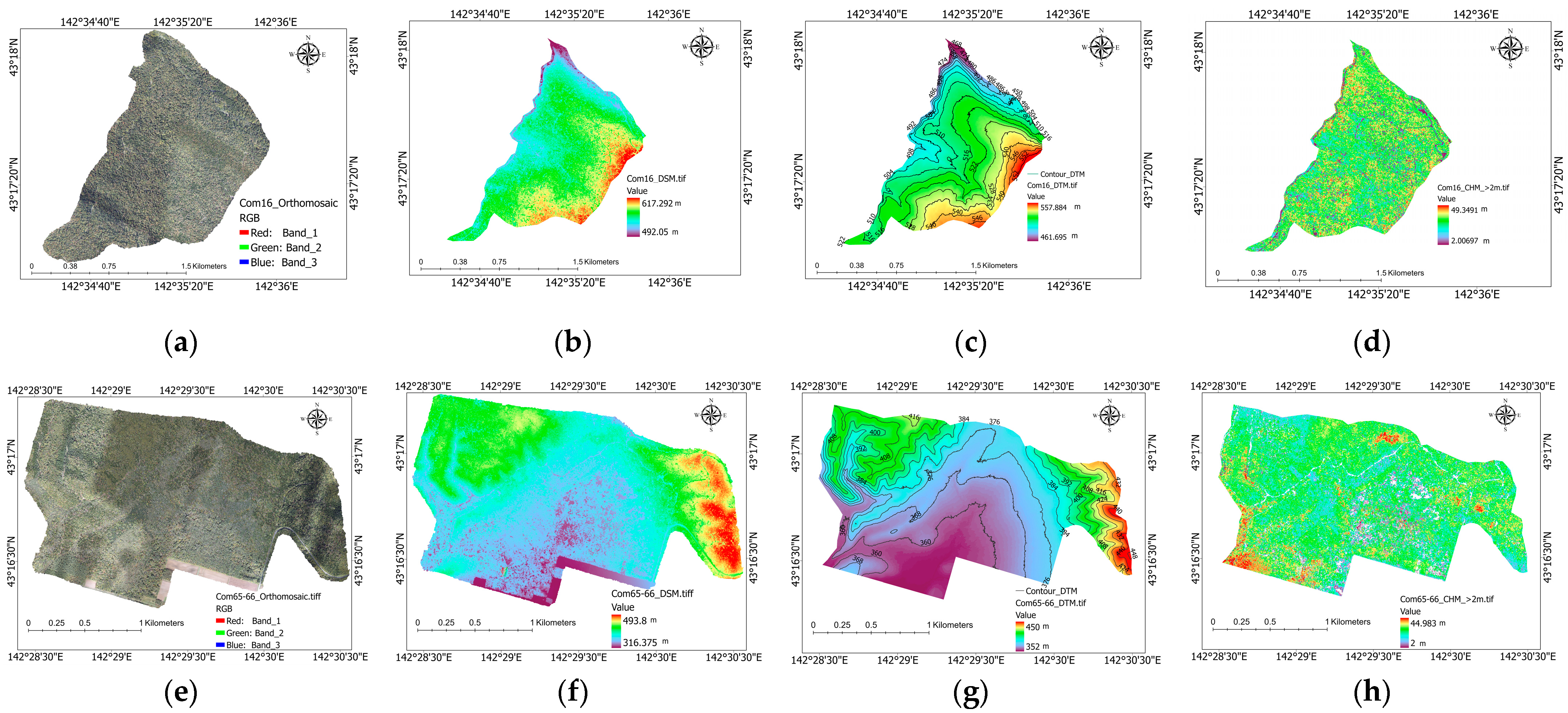
3.1. DSMs, DTMs, CHMsm and Orthomosaics
Figure 6 shows the CHMs, DSMs, and DTMs alongside the orthomosaics derived from comp16 and comp65-66. In com16, height ranges in the DSM, DTM, and CHM were 492.05–617.29, 461.70–557.70, and 2.00–49.35 m, respectively. For comp65-66, these ranges were 316.38–493.80, 352.00–450.00, and 2–44.98 m, respectively. The mean slope of com16 was 7.13° (range: 0.02°–62.05°), while that of com65-66 was 5.97° (range 0.00°–65.90°).

Figure 6.
Illustration of CHM derived from DSM and LiDAR DTM with orthomosaic in the forest compartments: (a) orthomosaic of comp16; (b) DSM of comp16; (c) DTM of comp16; (d) CHM of comp16; (e) orthomosaic of comp65-66; (f) DSM of comp65-66; (g) DTM of comp65-66; (h) CHM of comp65-66.
3.2. Variable Selection
Table 4 shows the predictor variables (structural and textural metrics from CHM and spectral metrics from orthomosaics) that achieved the best accuracy (Table 5) for the field forest structural parameters: Hd, DBH, BA, V, CST, Sden, and BLr. MLR and RF models utilized these variables to predict forest structural parameters accurately. Both models selected suitable variables from structural, textural, and spectral metrics. In general, all structural and textual variables, along with most spectral variables, were chosen to predict field forest structural parameters. The RF outperformed the MLR, although MLR demonstrated higher accuracy for BA in comp16.

Table 4.
Selected variables in MLR and RF models for forest structural parameters in comp16 and comp65-66.

Table 5.
Value of R2 and RMSE for MLR and RF models for forest structural parameters estimation in comp16 and comp65-66.
3.3. Accuracy of Forest Structural Parameters
3.3.1. Dominant Tree Height
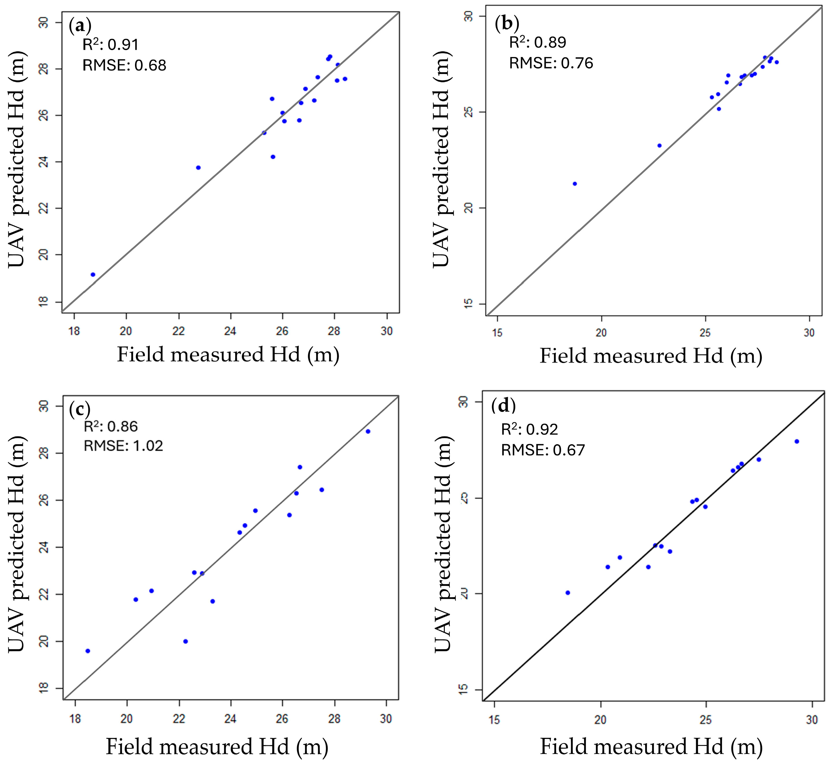
Figure 7 shows the field-measured Hd alongside the UAV-predicted Hd for the two forest compartments and the two models (RF and MLR). The R2 value for the mean Hd was 0.86–0.92; the RMSE was 0.61–1.02. The RF model achieved the highest Hd accuracy for com65-66 (R2 = 0.92, RMSE = 0.67). In com65-66, Hd accuracy surpassed that of other field parameters for both models (R2 = 0.86–0.92, RMSE = 0.67–1.02). The RF model performed well in predicting Hd (R2 = 0.89–0.92, RMSE = 0.67–0.76). CHM structural metrics (CHM max and >P50, >CD25), together with certain textural (s_Avg, ASM) and spectral (nR) metrics, were selected to predict Hd (Table 4).
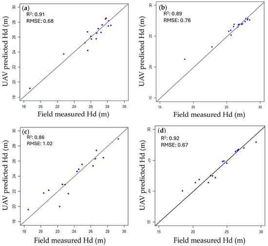
Figure 7.
Field–measured Hd versus UAV–predicted Hd: graphs (a,b) show the results in comp16, while (c,d) represent the results in comp65-66; (a,c) display the results of MLR, while (b,d) show the results of RF.
3.3.2. Tree Diameter at Breast Height
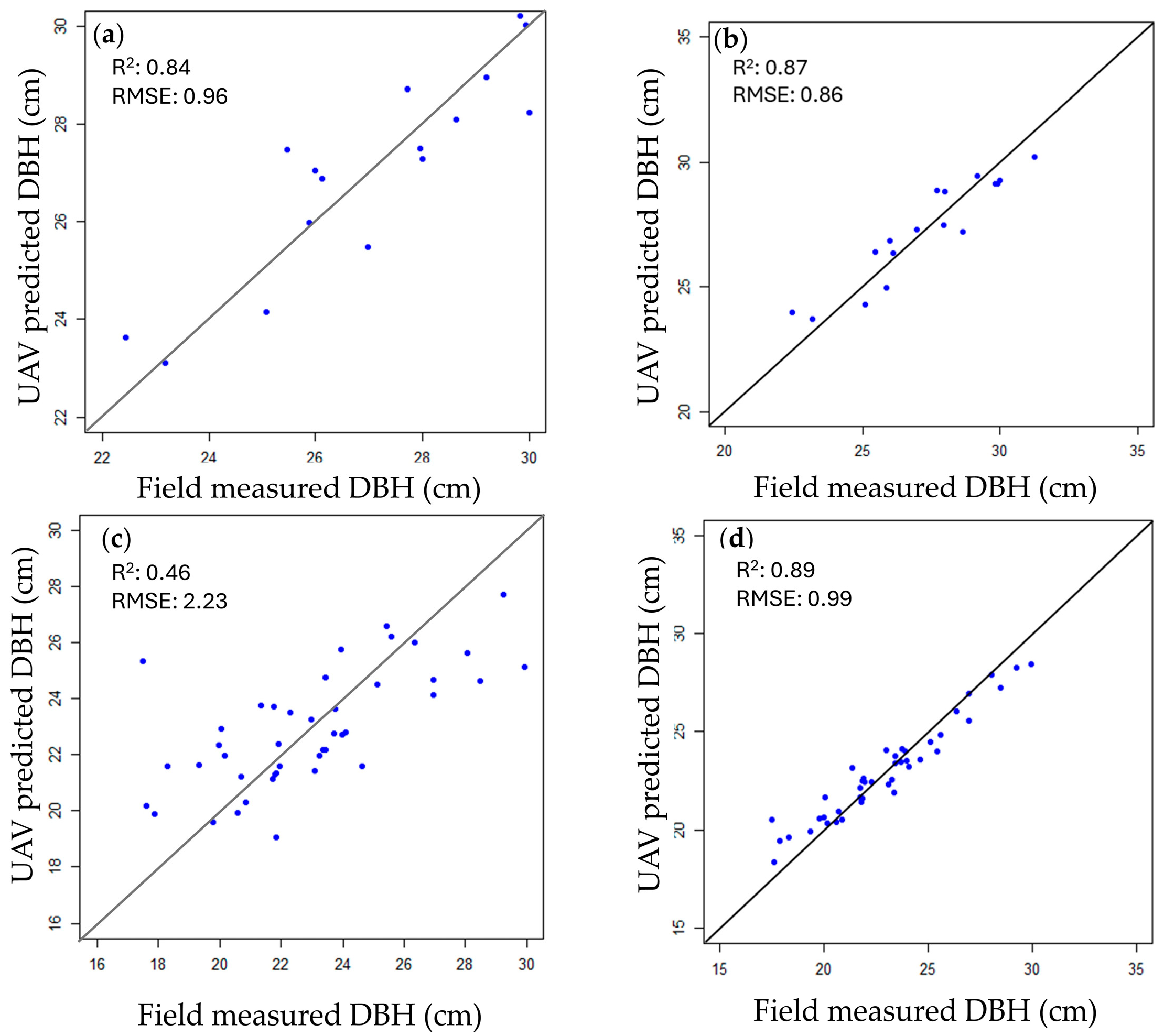
Figure 8 illustrates the relationship between field-measured DBH and UAV-predicted DBH. Across both forest compartments and models, the R2 value for the mean DBH was 0.45–0.89; the RMSE was 0.86–2.23. In com16, MLR achieved high DBH prediction accuracy (R2 = 0.84, RMSE = 0.96), while RF yielded the highest accuracy in com65-66 (R2 = 0.89, RMSE = 0.99). Predictor variables for DBH included CHM structural metrics (CHM max, CHM cv, >P50, >CD 50), along with spectral metrics (nR, nG) (Table 4).
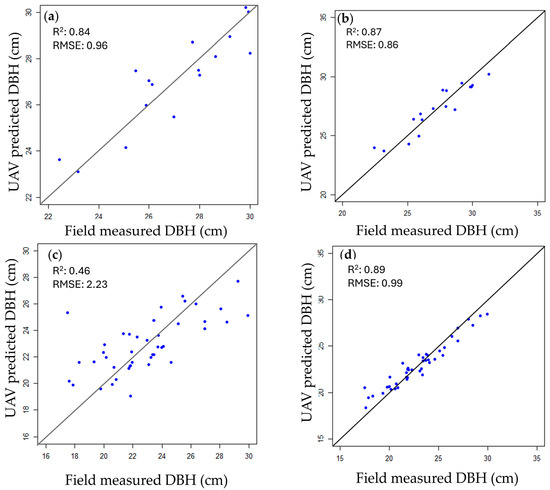
Figure 8.
Field–measured DBH versus UAV–predicted DBH: graphs (a,b) show the results in comp16, while (c,d) represent the results in comp65-66; (a,c) display the results of MLR, while (b,d) show the results of RF.
3.3.3. Basal Area
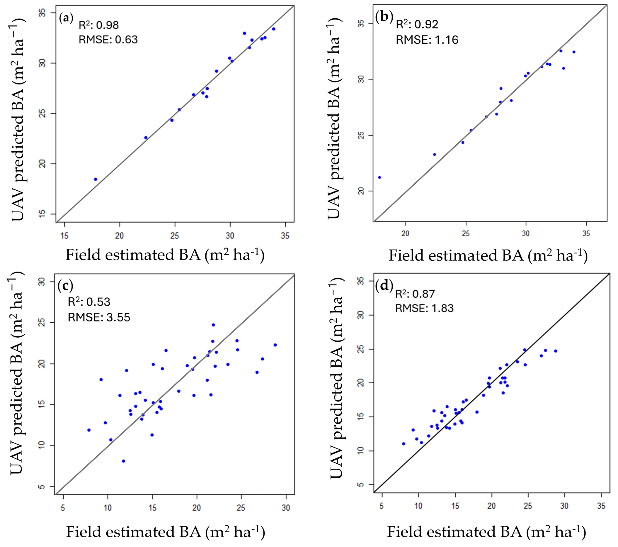
Figure 9 displays the relationship between field-estimated and UAV-predicted BA. Across both forest compartments and models, the mean R2 value for BA ranged from 0.53 to 0.98, with RMSE values between 0.63 and 3.55. In com16, the MLR model achieved the highest prediction accuracy (R2 = 0.98, RMSE = 0.63). For the compartment, BA prediction accuracy for both models was high (R2 = 0.92–0.98, RMSE = 0.63–1.16), surpassing that of Hd. However, only RF performed well in com65-66 (R2 = 0.87, RMSE = 1.83). CHM structural (CHM max, CHM cv, CHM mean, >P25, >CD50), textural (Cont, s_Avg), and spectral metrics (nR, nRBVI, B/R, nGBVI, nB, nR) were selected to predict BA (Table 4).
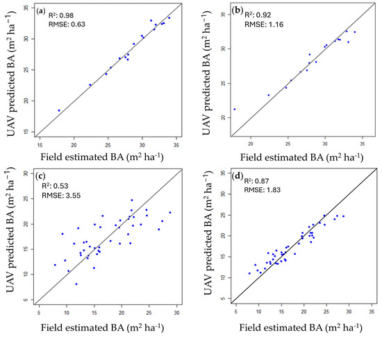
Figure 9.
Field–estimated BA versus UAV–predicted BA: graphs (a,b) show the results in comp16, while (c,d) represent the results in comp65-66; (a,c) display the results of MLR, while (b,d) show the results of RF.
3.3.4. Volume
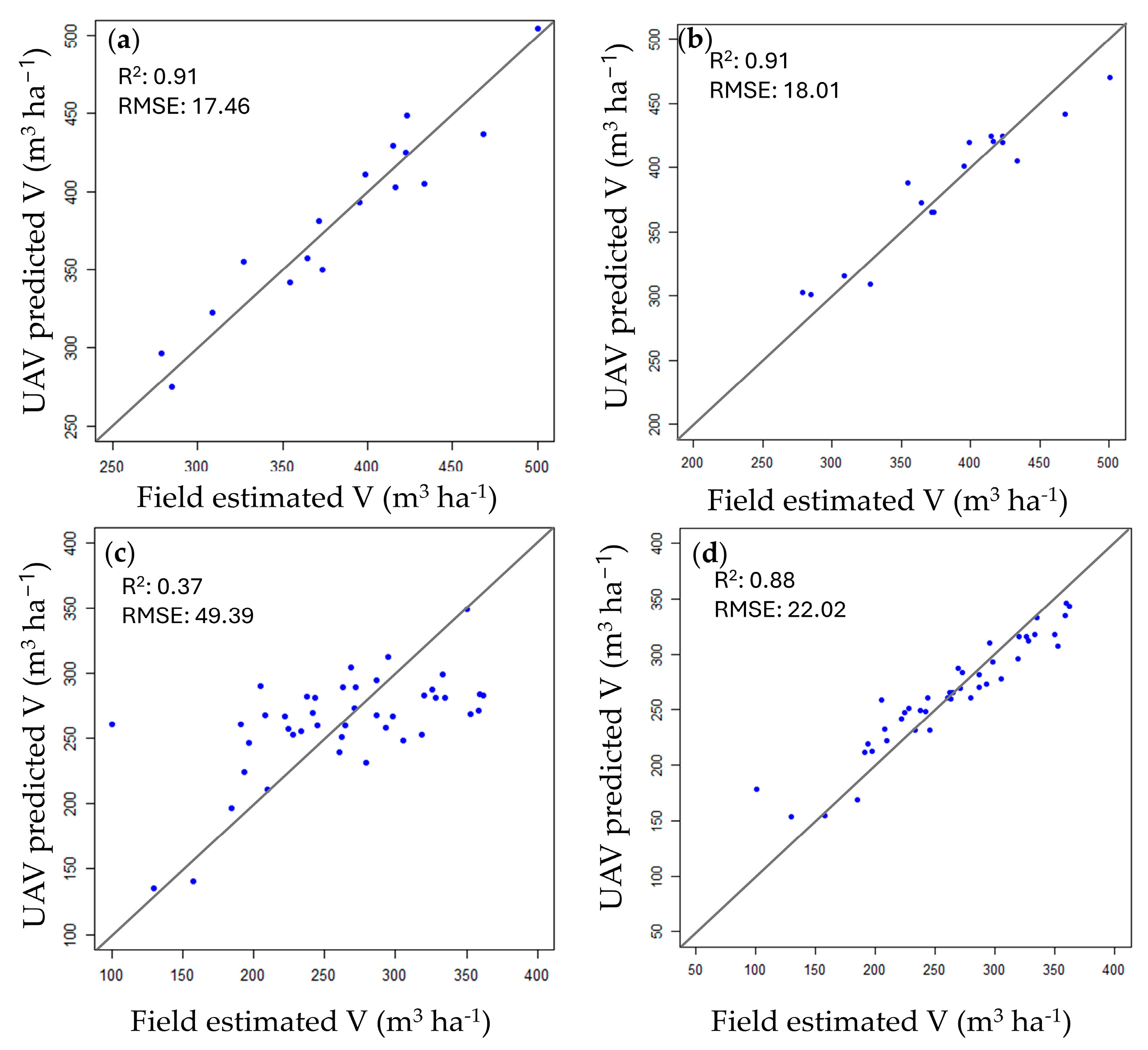
The comparison between field-estimated and UAV-predicted V is shown in Figure 10. Across both forest compartments and models, the R2 value for the mean V was 0.37–0.91; the RMSE was 17.46–49.39. In comp65-66, the RF model demonstrated the highest V prediction accuracy (R2 = 0.88, RMSE = 22.02). However, for both models, V prediction accuracy was higher in com16 than in com65-66 (R2 = 0.91, RMSE = 17.46–18.01). Predictor variables for volume included structural (CHM mean, CHM max, CHM_cv, >P25, >CD50), textural (s_Avg), and spectral metrics (nR) (Table 4).
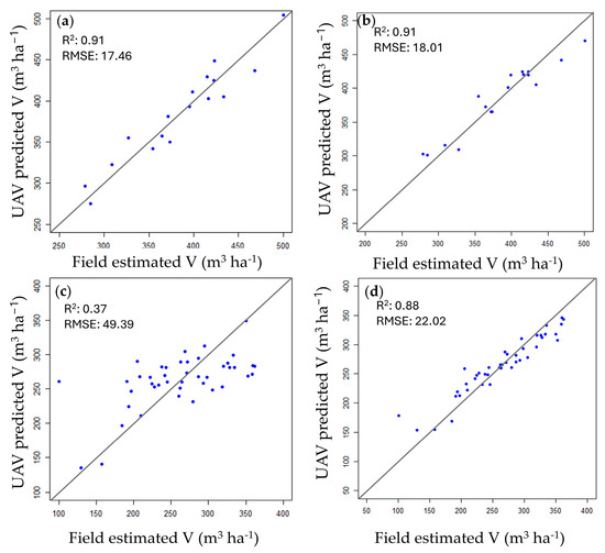
Figure 10.
Field–estimated V versus UAV–predicted V: graphs (a,b) show the results in comp16, while (c,d) represent the results in comp65-66; (a,c) display the results of MLR, while (b,d) show the results of RF.
3.3.5. Carbon Stock
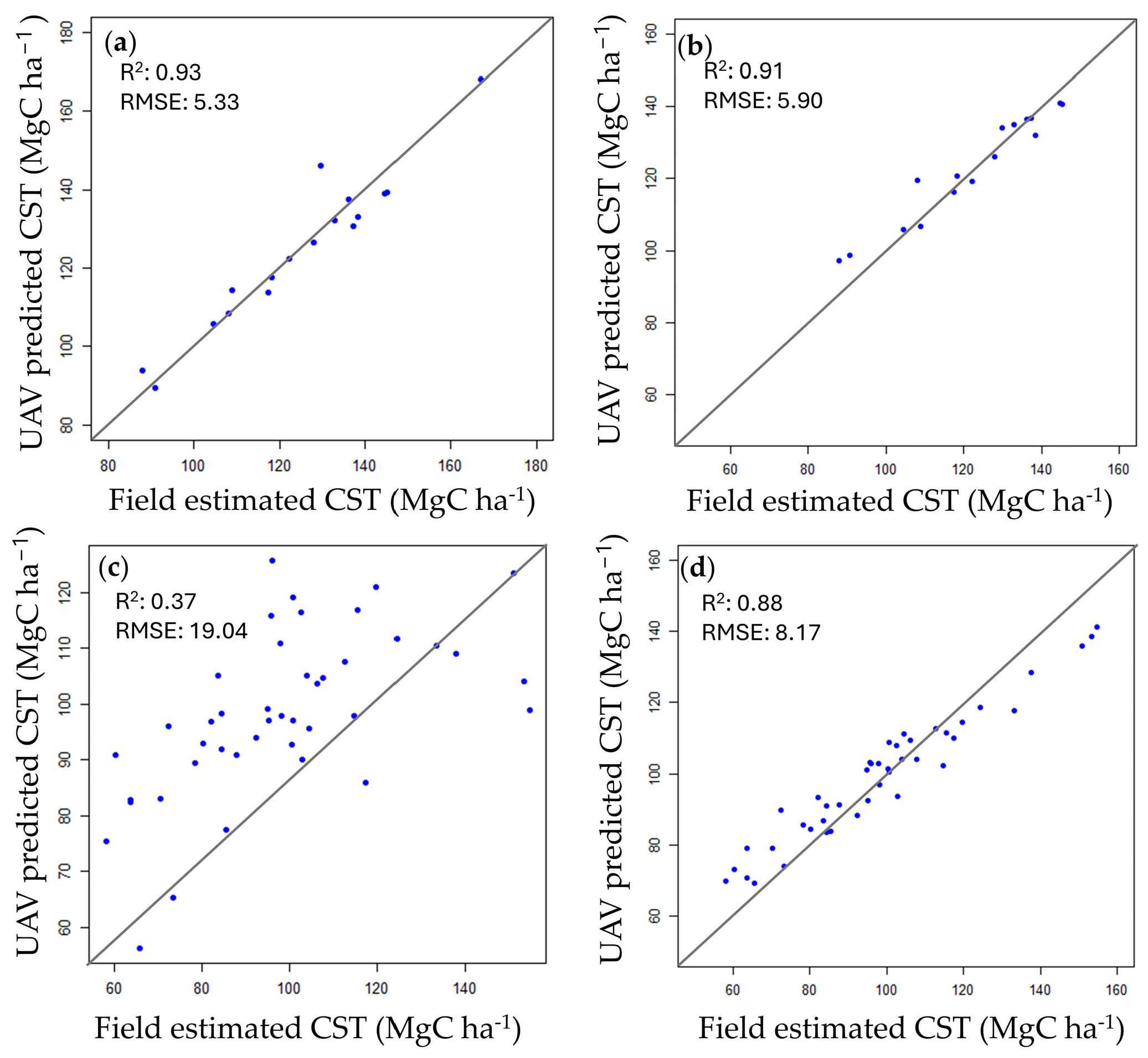
Figure 11 shows the relationship between field-estimated and UAV-predicted CST. For the two forest compartments and the two models, the R2 value for the mean CST was 0.37–0.93; the RMSE was 5.33–19.04. In comp16, the highest prediction accuracy for CST was achieved with MLR (R2 = 0.93, RMSE = 5.53) and RF (R2 = 0.91, RMSE = 5.90). The model selected structural (CHM mean, CHM max, CHM cv, >P25, >CD50), textural (Cont, s_Avg, Var, d_Var, Roug), and spectral metrics (nR, nB, VARI) as predictor variables for CST (Table 4).
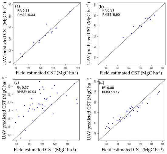
Figure 11.
Field–estimated CST versus UAV–predicted CST: graphs (a,b) show the results in compartment 16, while (c,d) represent the results in compartment 65-66; (a,c) display the results of MLR, while (b,d) show the results of RF.
3.3.6. Stem Density
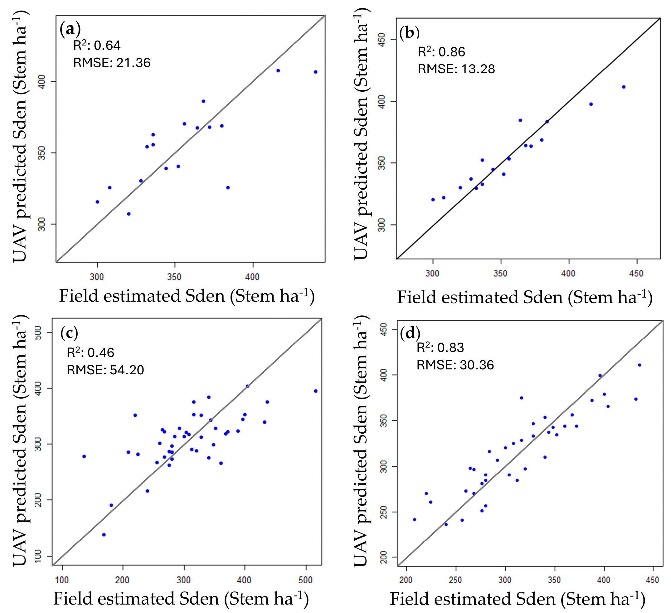
Figure 12 illustrates the comparison between field-estimated and UAV-predicted Sden. Across both forest compartments and the two models, the R2 value for the mean Sden ranged from 0.46 to 0.86, with RMSE values between 13.28 and 54.20. The RF model demonstrated the highest prediction accuracy for Sden (R2 = 0.83–0.86, RMSE = 13.28–30.36) in both compartments. Predictor variables selected for Sden included structural (CHM max, CHM cv, >75CD), textural (Cont, d_Ent, ASM), and spectral metrics (nRBVI, nR, nGBVI, B/R) (Table 4).

Figure 12.
Field–estimated Sden versus UAV–predicted Sden: graphs (a,b) show the results in comp16, while (c,d) represent the results in comp65-66; (a,c) display the results of MLR, while (b,d) show the results of RF.
3.3.7. Broadleaf Ratio
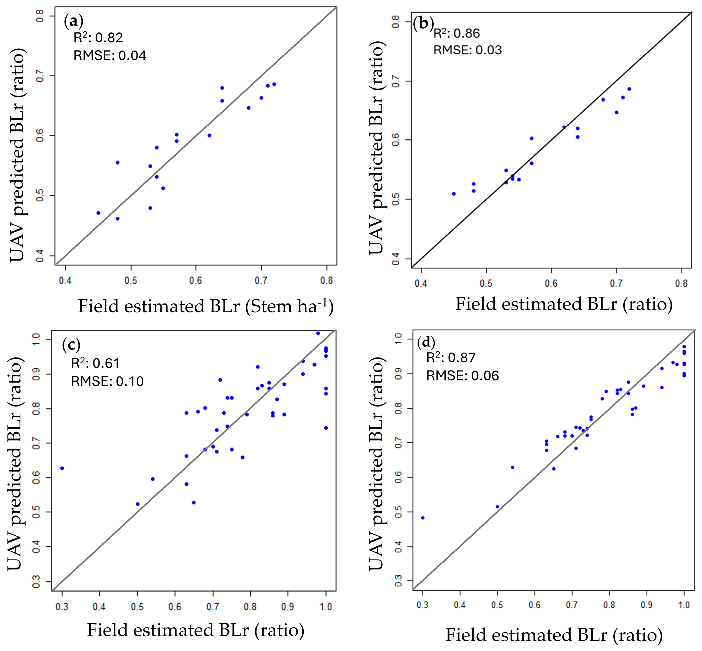
Figure 13 shows the comparison between field-estimated BLr and UAV-predicted BLr. Across both forest compartments and the two models, the R2 value for (BLr) was 0.61–0.87; the RMSE was 0.06–0.10. In com16, both MLR and RF performed well in accurately predicting BLr (R2 = 0.82–0.86, RMSE = 0.03–0.04), while only RF achieved good performance in com65-66 (R2 = 0.87, RMSE = 0.06). Predictor variables selected for BLr included structural (>25CD, P50, CHM max, CHM cv), textural (Corr, Cont, s_Avg, d_Var, ASM, Roug), and spectral metrics (nR, nRBVI, B/G, nB) (Table 4).

Figure 13.
Field–estimated field BLr versus UAV–predicted BLr: graphs (a,b) show the results in comp16, while (c,d) represent the results in comp65-66; (a,c) display the results of MLR, while (b,d) show the results of RF.
4. Discussion
4.1. Variable Selection
In contrast to LiDAR point clouds, UAV SfM yields relatively lower estimation accuracy due to the canopy occlusion [34,42]. However, different UAV metrics and high-resolution imagery offer relatively higher estimation accuracy, particularly with RGB imagery. In this study, we extracted structural, textural, and spectral metrics from high spatial resolution RGB imagery to predict forest structural parameters [33]. The classification accuracy of land use improves with high spatial resolution remote sensing images (>1.65 m/pixel) in heterogeneous forests using spectral and textural features [37,40]. We employed high-resolution CHMs (0.5 m/pixel), consistent with previous studies [29,31] to predict the field forest structural parameter in inventory plots. The extraction of spectral metrics from high resolution provided higher estimation accuracy [38,41]. In this study, we used very high-resolution RGB orthomosaics (1.6 cm/pixel) to extract spectral metrics. However, the use of CHM structural metrics with high-resolution RGB imagery did not provide high estimation accuracy for complex mixed conifer–broadleaf forests [29]. Estimations of forest structure are also dependent on ambient environmental conditions, such as light availability, sunshine, rainfall, wind, water resources, and soil properties, which strongly influence the structural, textural, and spectral properties of the forest. Therefore, assessing the metrics representing these properties enhances estimation accuracy [65]. In this study, we combined different textural and structural metrics of CHM with spectral metrics of orthomosaics. Incorporating all three metrics, both RF and MLR provided relatively high estimation accuracy for all forest structural parameters. While we used a default window size of 3 m × 3 m to extract forest structural and textural metrics from CHMs, estimation accuracy could be further improved by using other window sizes. For example, a previous study reported that a window size of ≤9 m × 9 m performed well in extracting textual metrics from satellite imagery [39].
4.1.1. Structural Variables
Pearson’s correlation (r) test was performed to assess the correlations between the field parameters and UAV metrics [22]. Most of the CHM’s structural metrics correlated significantly with field structural parameters, making them more frequently selected by the models (>0.7, p < 0.001) than either the textural or the spectral metrics. Similar UAV RGB and LiDAR structural metrics (P95, P75, CD, and CHM max) were chosen in previous studies for predicting forest structural parameters [34]. In our study, CHM max, >P50, and >CD25 were selected to predict Hd, representing the vertical distribution of canopy top and serving as a predictor of forest biomass [41]. While P represents the measurement of the vertical height of the pixel, CD indicates the proportion of the pixel percentage. Hd in a complex forest depends on factors such as spacing, surrounding species, canopy closure, and other environmental conditions, thus correlating with these metrics [14,34,35]. The UTHF’s adoption of single tree level management for high-value timber species [69] highlights the importance of identifying dominant trees in the canopy layers for tree selection. Mapping Hd distribution can facilitate the identification of the largest trees.
Similar patterns were observed for V and CST (>0.6, p < 0.001) in both compartments, as indicated by the MLR and RF models, aligning with the strong correlation between these parameters. This trend was also evident for DBH and BA (>0.6 at p < 0.001) due to the dependence of BA on DBH. DBH and BA represent the horizontal distribution of the forest and are better explained by structural metrics. DBH is crucial for assessing tree value in timber selection [69], underscoring the importance of identifying its distribution in the study area. BA, being an area measure, carries more weight than DBH in spatial distribution. Given their strong correlation, similar structural metrics were selected for DBH and BA (CHM max, CHM mean, CHM cv, >P25, and >CD50). Similarly, V and CST represent the unified distribution and were predicted using the same structural metrics (CHM mean, CHM max, CHM cv, >P25, and >CD50). Individual tree detection, based on canopy top estimation, influenced Sden estimation [70], explaining why Sden was predicted by CHM max.
4.1.2. Textual Variables
The inclusion of textural metrics alongside structural metrics contributed to the enhanced accuracy of forest structural parameter predictions [26,39]. In a study by Ozdemir and Karnieli [26], WordView-2 satellite imagery was used to estimate forest structural parameters, yielding comparable accuracies for Sden (R2 = 0.38, RMSE = 109.56), BA (R2 = 0.54, RMSE = 1.79), and V (R2 = 0.42, RMSE = 27.18). Particularly strong correlations were observed between the standard deviation of the DBH and the contrast of the red band (r = 0.75, p < 0.01), as well as between BA and the entropy of the blue band (r = 0.73, p < 0.01) [26].
In this study, Ent, d_Ent, Var, d_Var, and s_Avg were first-order textural metrics, while ASM, Cont, and Corr were second-order textural metrics. Higher values of Ent, d_Ent Var, d_Var, and Roug indicate greater complexity in forest structure, whereas a high ASM value represents the uniformity in forest structure. Additionally, Cont and Corr values are increased when the scale value (size of the spatial features) exceeds the distance (spacing between different elements) [26,40,53,55]. The selection of textural metrics depended on the nature of the response variable. In both compartments, s_Avg played a significant role in estimating many structural parameters. s_Avg calculates the average gray-level intensity of the sum of pixel pairs within the moving window. Similarly, BA, V, CST, Sden, and BLr were estimated based on the average of sum value per plot, indicating their ability to explain the horizontal and unified distributions of the forest structural parameters in our study. Meng et al. [39] noted that first-order textural metrics were not more strongly correlated with forest field structural variables than second-order textual metrics, which could be attributed to the spatial resolution of the satellite imagery. Textural metrics such as d_Ent, Ent, ASM, Corr, Roug, and Cont selected as predictors in this study, serve as indicators of structural complexity. Meng et al. [39] also found that textual variables, such as max difference, homogeneity, ASM, Corr, Ent, Cont, dissimilarity, and Var, predicted the BA, quadratic mean diameter (QMD), V, and Sden.
4.1.3. Spectral Variables
Greater accuracy in predicting forest structural parameters was achieved through the inclusion of spectral metrics alongside structural metrics, as evidenced by the selection of many spectral metrics by both MLR and RF models. In com16, normalized R (nR) was chosen to predict the forest structural parameters, while in com65-66, most spectral metrics were selected. RF selected nearly all spectral metrics to predict BA, V, CST, Sden, and BLr. The visible spectrum’s R and B bands, representing tree growth, exerted significant influence on forest structural parameters, particularly height and DBH. Spectral metrics are strongly influenced by vegetation pigments, physiology, and stress, thereby impacting forest structural attributes [38]. In a study by Castillo-Santiago et al. [36], spectral metrics were not selected to predict BA, V, or AGB, contrasting with our findings. However, metric selection is dependent on forest conditions and imagery type, differing from our study. Wallner et al. [71] found that conifer stands were represented by fewer spectral metrics, while broadleaved forests with closed canopies required a larger number of indices. This could explain why only nR was selected in com16, whereas a large number of metrics were chosen in com65-66 [39].
4.2. Accuracy of Forest Structural Parameters
High accuracy in predicting forest structural parameters across both compartments was achieved using RF (R2 = 0.83–0.92) and MLR (R2 = 0.37–0.98) models using UAV RGB imagery. This success was attributed to employing high-resolution orthomosaics and CHMs, along with various UAV metrics.
Our findings align with previous studies on estimating forest structural parameters in complex forests. For instance, MLR achieved higher prediction accuracy for Hd in both compartments (R2 = 0.86–0.91, RMSE = 0.68–1.02) compared to Jayathunga et al. [34], who used a GLMM with UAV RGB (R2 = 0.82, RMSE = 1.78) and LiDAR point clouds (R2 = 0.87, RMSE = 1.5), attributing use differences to structural metrics and fixed-wing UAV [29]. Similarly, DBH accuracy was higher in com16 (R2 = 0.84, RMSE = 0.96) compared to com65-66 (R2 = 0.46, RMSE = 2.23), consistent with Jayathunga et al. [34], who used UAV RGB (R2 = 0.64, RMSE = 3.92) and airborne LiDAR (R2 = 0.61, RMSE = 3.75) and focused on QMD. Higher prediction accuracy for BA in com16 (R2 = 0.98. RMSE = 0.63) compared to com65-66 (R2 = 0.53, RMSE = 3.55) using MLR was also similar to Jayathunga et al. [34] results for UAV RGB (R2 = 0.74, RMSE = 5.42) and LiDAR point clouds (R2 = 0.81, RMSE = 4.58).
Furthermore, our study demonstrated higher accuracy for Sden in both com16 (R2 = 0.64, RMSE = 21.36) and com65-66 (R2 = 0.46, RMSE = 54.20) using the MLR models, contrasting with Jayathunga et al. [34], who reported a lower Sden for both UAV RGB (R2 = 0.37, RMSE = 78) and LiDAR (R2 = 0.35, RMSE = 76).
Predicting V by both MLR and RF showed similar accuracy (R2 = 0.91, RMSE = 17.46–18.01) in com16. The RF model achieved higher accuracy for V (R2 = 0.88, RMSE = 22.02) and CST (R2 = 0.88, RMSE = 8.17) in com65-66 compared to a previous study (V: R2 = 0.84 and RMSE = 39.8; CST: R2 = 0.82, RMSE = 14.3) using UAV SfM [29], and in a study in other areas in Japan [27], both for V (R2 = 0.76, RMSE = 16.4; R2 = 0.80, RMSE = 55.04) [72] and CST (R2 = 0.78, RMSE = 22.68) using LiDAR point clouds and GLMMs [72]. However, our results align with those previously reported for other compartments using metrics derived from LiDAR point clouds, with accuracies for V (R2 = 0.85, RMSE = 38.9) and CST (R2 = 0.81, RMSE = 13.6) [29]. A study utilizing UAV SfM found that incorporating one image metric (broadleaf cover percentage) alongside structural metrics improved the estimation accuracy, whereas when this metric was excluded, a decrease in R2 was observed for both V (R2 = 0.81) and CST (R2 = 0.79) without any alterations in RMSE [29]. In our study, the integration of various spectral and textural metrics improved the prediction accuracy of V and CST. Jayathunga et al. [30], focusing on other compartments in the study area, obtained the highest accuracy for biomass estimation using LiDAR-derived point clouds in an RF model (R2 = 0.94, RMSE = 12), and their MLR results align with our MLR results (R2 = 0.85, RMSE = 18.1). Conversely, Zhang et al. [73] reported a relatively low prediction accuracy for CST (R2 = 0.66, RMSE = 48.51) in a study of a tropical dense forest, utilizing CHM metrics and UAV SfM point clouds with an RF model.
In their examination of a complex subtropical forest using LiDAR point clouds, Zhang et al. [22] reported the highest accuracy for HL (adjusted R2 = 0.61–0.88) and AGB (adjusted R2 = 0.54–0.81), followed by V (adjusted R2 = 0.42–0.78), DBH (adjusted R2 = 0.48–0.74), and BA (adjusted R2 = 0.41–0.69), and a lower accuracy was obtained for Sden (adjusted R2 = 0.39–0.64). In contrast, our study achieved accurate prediction for all parameters, including Sden, attributed to the utilization of structural, textural, and spectral metrics as predictor variables in RGB imagery analyses. Despite the subtropical forest context, where UAV SfM point clouds were combined with P, CD, canopy V, and Weibull metrics, our accuracy levels remained comparable with HL (R2 = 0.92, relative RMSE (rRMSE) = 5.71), DBH (R2 = 0.83, rRMSE = 10.43), V (R2 = 0.77, rRMSE = 16.89), and AGB (R2 = 0.78, rRMSE = 13.73). Notably, our RMSE values for Hd and BA were lower than those reported in a separate study using UAV SfM point clouds, while the V value remained consistent [28,74,75]. Furthermore, our RMSE values for HL (1.13) and V (118.3) were lower than those obtained in an analysis of a managed temperate coniferous forest using UAV SfM point clouds [18].
We observed that both RF (R2 = 0.86–0.87, RMSE = 0.06–0.03) and MLR (R2 = 0.61–0.82, RMSE = 0.04–0.10) performed effectively in predicting BLr. The sole use of BLr as a response variable enabled predictions for regions dominated by broadleaf trees. The inclusion of broadleaf vegetation cover enhanced the explanatory capacity in the regression analysis for V and CST [29]. In a study by Yang et al. [76] analyzing conifer BLr using Fifteen Gaofen-1 satellite data, lower accuracy (83.5%) was achieved compared to our findings.
The prediction accuracy of forest structural parameters was higher in com16 than in com65-66, likely due to several factors, including a smaller number of plots in com16 and differences in stand type, species dominance, and other site characteristics (Figure 2). Jayathunga et al. [34] analyzed the influence of topographical features on the estimation of forest structural parameters and found a statistically significant association between the two analyzed compartments. The extensive wind damage in com65-66 in 1981 may also contribute to the high variability in forest structure across the study area, potentially leading to the lower prediction accuracy observed for com65-66 compared to com16 [26,34]. Further, conifer-dominated plots were more abundant in com16 (12/17), while broadleaf-dominated plots were more common in com65-66 (30/43). This was confirmed in the stand classification map of the UTHF (Figure 2), with com16 mostly comprising conifer-dominated stands and com65-66 showing a prevalence of broadleaf and plantation stand types. This difference likely contributes to the variation in prediction accuracy of forest structural parameters across the study area. Jayathunga et al. [30] reported a higher accuracy for biomass in a conifer forest (R2 = 0.87, RMSE = 22.7) compared to broadleaf forest (R2 = 0.90, RSME = 32.1) using LiDAR point cloud metrics. Further studies focusing on forest structural parameter estimations based on stand type are needed, potentially including a larger number of sampling plots in each category.
5. Conclusions
In conclusion, our study demonstrates the effectiveness of utilizing structural, textural, and spectral metrics derived from UAV RGB imagery for improving the estimation of forest structural parameters in a mixed conifer–broadleaf forest using RF and MLR models. Structural and textural metrics were derived from CHMs, while spectral metrics were obtained from orthomosaics. The integration of all three types of metrics by the models provided high explanatory power, enhancing the accuracy of forest structural parameter predictions in a complex mixed conifer–broadleaf forest. The number of variables selected by the models varied depending on the field forest structural parameters.
The RF model demonstrated excellent performance for all field forest structural parameters across the study area, whereas for the MLR model, performance was excellent only for Hd, BA, and CST in com16. Prediction accuracies achieved with RF for Hd, DBH, V, CST, Sden, and BLr were comparable to those in previous studies, while MLR showed slightly higher prediction accuracies for BA in com16. Our findings align with studies that utilized LiDAR-derived point clouds to estimate forest structural parameters in a complex forest, offering insights that could enhance estimation accuracy when employing RGB imagery, SfM technology, and diverse structural, textural, and spectral metrics. Future research endeavors should focus on integrating RGB spectral metrics with multispectral imagery and employing various machine learning techniques to further improve estimations of forest structural parameters. Mapping of forest structural parameters at a spatial scale using wall-to-wall mapping will be instrumental in supporting sustainable forest management practices.
Author Contributions
Conceptualization, methodology, formal analysis, and writing (original draft preparation), J.K.; resources, supervision, writing, review, and editing, T.O.; writing, review and editing, S.T.; writing, review, and editing, T.H. All authors have read and agreed to the published version of the manuscript.
Funding
The LiDAR data were provided by the UTHF from the datasets funded by JURO KAWACHI DONATION FUND, the grant of joint research between the UTHF and Oji Forest and Products Co., Ltd., and Japan Society for the Promotion of Science (JSPS) KAKENHI No. 16H04946. This work was conducted as part of a Ph.D. program funded by Japan International Cooperation Agency (JICA) under the SDGs Global Leader Program (JFY 2022) through JICA Knowledge Co-Creation Program (Long-Term Training) D2203615-202006551-J011.
Data Availability Statement
The field and UAV datasets presented in this study are available on request from the corresponding author.
Acknowledgments
We would like to thank the technical staff of the UTHF—Masaki Matsui, Noriyuki Kimura, Nozomi Oikawa, Shinya Inukai, Koichi Takahashi, Satoshi Chiino, Masaki Tokuni, Kenji Fukushi, and Yuji Nakagawa—for their significant contribution in field measurements and UAV data collection at the study site. ChatGPT (OpenAI, San Francisco, CA, USA) provided assistance in English editing.
Conflicts of Interest
The authors declare no conflicts of interest.
Appendix A

Figure A1.
Diameter class distribution: (a) diameter class distribution of conifer and broadleaf in com16; (b) diameter class distribution of conifer and broadleaf com65-66; (c) diameter class distribution of forest types in com16; (d) diameter class distribution of forest types in com65-66.
Figure A1.
Diameter class distribution: (a) diameter class distribution of conifer and broadleaf in com16; (b) diameter class distribution of conifer and broadleaf com65-66; (c) diameter class distribution of forest types in com16; (d) diameter class distribution of forest types in com65-66.
References
- Seidler, R.; Bawa, K.S. Biodiversity in Logged and Managed Forests. In Encyclopedia of Biodiversity; Elsevier: Amsterdam, The Netherlands, 2013; pp. 446–458. [Google Scholar]
- Palace, M.W.; Sullivan, F.B.; Ducey, M.J.; Treuhaft, R.N.; Herrick, C.; Shimbo, J.Z.; Mota-E-Silva, J. Estimating Forest Structure in a Tropical Forest Using Field Measurements, a Synthetic Model and Discrete Return Lidar Data. Remote Sens. Environ. 2015, 161, 1–11. [Google Scholar] [CrossRef]
- Franklin, J.F.; Spies, T.A.; Van Pelt, R.; Carey, A.B.; Thornburgh, D.A.; Berg, D.R.; Lindenmayer, D.B.; Harmon, M.E.; Keeton, W.S.; Shaw, D.C.; et al. Disturbances and Structural Development of Natural Forest Ecosystems with Silvicultural Implications, Using Douglas-Fir Forests as an Example. For. Ecol. Manag. 2002, 155, 399–423. [Google Scholar] [CrossRef]
- Frey, J.; Kovach, K.; Stemmler, S.; Koch, B. UAV Photogrammetry of Forests as a Vulnerable Process. A Sensitivity Analysis for a Structure from Motion RGB-Image Pipeline. Remote Sens. 2018, 10, 912. [Google Scholar] [CrossRef]
- Zielewska-Büttner, K.; Adler, P.; Ehmann, M.; Braunisch, V. Automated Detection of Forest Gaps in Spruce Dominated Stands Using Canopy Height Models Derived from Stereo Aerial Imagery. Remote Sens. 2016, 8, 175. [Google Scholar] [CrossRef]
- Seidel, D.; Ehbrecht, M.; Puettmann, K. Assessing Different Components of Three-Dimensional Forest Structure with Single-Scan Terrestrial Laser Scanning: A Case Study. For. Ecol. Manag. 2016, 381, 196–208. [Google Scholar] [CrossRef]
- Shimizu, K.; Nishizono, T.; Kitahara, F.; Fukumoto, K.; Saito, H. Integrating Terrestrial Laser Scanning and Unmanned Aerial Vehicle Photogrammetry to Estimate Individual Tree Attributes in Managed Coniferous Forests in Japan. Int. J. Appl. Earth Obs. Geoinf. 2022, 106, 102658. [Google Scholar] [CrossRef]
- White, J.C.; Coops, N.C.; Wulder, M.A.; Vastaranta, M.; Hilker, T.; Tompalski, P. Remote Sensing Technologies for Enhancing Forest Inventories: A Review. Can. J. Remote Sens. 2016, 42, 619–641. [Google Scholar] [CrossRef]
- Tomppo, E.; Gschwantner, T.; Lawrence, M.; McRoberts, R.E.; Gabler, K.; Schadauer, K.; Vidal, C.; Lanz, A.; Ståhl, G.; Cienciala, E. National Forest Inventories Pathways for Common Reporting; Springer: Dordrecht, The Netherlands, 2010; Volume 1, pp. 541–553. [Google Scholar]
- Neuville, R.; Bates, J.S.; Jonard, F. Estimating Forest Structure from UAV-Mounted LiDAR Point Cloud Using Machine Learning. Remote Sens. 2021, 13, 352. [Google Scholar] [CrossRef]
- Cao, L.; Liu, K.; Shen, X.; Wu, X.; Liu, H. Estimation of Forest Structural Parameters Using UAV-LiDAR Data and a Process-Based Model in Ginkgo Planted Forests. IEEE J. Sel. Top. Appl. Earth Obs. Remote Sens. 2019, 12, 4175–4190. [Google Scholar] [CrossRef]
- Bulut, S.; Günlü, A.; Çakır, G. Modelling Some Stand Parameters Using Landsat 8 OLI and Sentinel-2 Satellite Images by Machine Learning Techniques: A Case Study in Türkiye. Geocarto Int. 2023, 38, 2158238. [Google Scholar] [CrossRef]
- Karthigesu, J.; Owari, T.; Tsuyuki, S.; Hiroshima, T. UAV Photogrammetry for Estimating Stand Parameters of an Old Japanese Larch Plantation Using Different Filtering Methods at Two Flight Altitudes. Sensors 2023, 23, 9907. [Google Scholar] [CrossRef] [PubMed]
- Liu, K.; Shen, X.; Cao, L.; Wang, G.; Cao, F. Estimating Forest Structural Attributes Using UAV-LiDAR Data in Ginkgo Plantations. ISPRS J. Photogramm. Remote Sens. 2018, 146, 465–482. [Google Scholar] [CrossRef]
- Swayze, N.C.; Tinkham, W.T. Application of Unmanned Aerial System Structure from Motion Point Cloud Detected Tree Heights and Stem Diameters to Model Missing Stem Diameters. MethodsX 2022, 9, 101729. [Google Scholar] [CrossRef] [PubMed]
- Hoffrén, R.; Lamelas, M.T.; de la Riva, J. UAV-Derived Photogrammetric Point Clouds and Multispectral Indices for Fuel Estimation in Mediterranean Forests. Remote Sens. Appl. 2023, 31, 100997. [Google Scholar] [CrossRef]
- Wang, Y.; Pyörälä, J.; Liang, X.; Lehtomäki, M.; Kukko, A.; Yu, X.; Kaartinen, H.; Hyyppä, J. In Situ Biomass Estimation at Tree and Plot Levels: What Did Data Record and What Did Algorithms Derive from Terrestrial and Aerial Point Clouds in Boreal Forest. Remote Sens. Environ. 2019, 232, 111309. [Google Scholar] [CrossRef]
- Ota, T.; Ogawa, M.; Mizoue, N.; Fukumoto, K.; Yoshida, S. Forest Structure Estimation from a UAV-Based Photogrammetric Point Cloud in Managed Temperate Coniferous Forests. Forests 2017, 8, 343. [Google Scholar] [CrossRef]
- Puliti, S.; Ørka, H.; Gobakken, T.; Næsset, E. Inventory of Small Forest Areas Using an Unmanned Aerial System. Remote Sens. 2015, 7, 9632–9654. [Google Scholar] [CrossRef]
- Akinbiola, S.; Salami, A.T.; Awotoye, O.O.; Popoola, S.O.; Olusola, J.A. Application of UAV Photogrammetry for the Assessment of Forest Structure and Species Network in the Tropical Forests of Southern Nigeria. Geocarto Int. 2023, 38, 2190621. [Google Scholar] [CrossRef]
- Zhao, Y.; Im, J.; Zhen, Z.; Zhao, Y. Towards Accurate Individual Tree Parameters Estimation in Dense Forest: Optimized Coarse-to-Fine Algorithms for Registering UAV and Terrestrial LiDAR Data. GIsci. Remote Sens. 2023, 60, 2197281. [Google Scholar] [CrossRef]
- Zhang, Z.; Cao, L.; She, G. Estimating Forest Structural Parameters Using Canopy Metrics Derived from Airborne LiDAR Data in Subtropical Forests. Remote Sens. 2017, 9, 940. [Google Scholar] [CrossRef]
- Panagiotidis, D.; Abdollahnejad, A.; Slavík, M. 3D Point Cloud Fusion from UAV and TLS to Assess Temperate Managed Forest Structures. Int. J. Appl. Earth Obs. Geoinf. 2022, 112, 102917. [Google Scholar] [CrossRef]
- Panagiotidis, D.; Abdollahnejad, A.; Surový, P.; Chiteculo, V. Determining Tree Height and Crown Diameter from High-Resolution UAV Imagery. Int. J. Remote Sens. 2017, 38, 2392–2410. [Google Scholar] [CrossRef]
- Iglhaut, J.; Cabo, C.; Puliti, S.; Piermattei, L.; O’Connor, J.; Rosette, J. Structure from Motion Photogrammetry in Forestry: A Review. Curr. For. Rep. 2019, 5, 155–168. [Google Scholar] [CrossRef]
- Ozdemir, I.; Karnieli, A. Predicting Forest Structural Parameters Using the Image Texture Derived from WorldView-2 Multispectral Imagery in a Dryland Forest, Israel. Int. J. Appl. Earth Obs. Geoinf. 2011, 13, 701–710. [Google Scholar] [CrossRef]
- Ioki, K.; Imanishi, J.; Sasaki, T.; Morimoto, Y.; Kitada, K. Estimating Stand Volume in Broad-Leaved Forest Using Discrete-Return LiDAR: Plot-Based Approach. Landsc. Ecol. Eng. 2010, 6, 29–36. [Google Scholar] [CrossRef]
- White, J.; Stepper, C.; Tompalski, P.; Coops, N.; Wulder, M. Comparing ALS and Image-Based Point Cloud Metrics and Modelled Forest Inventory Attributes in a Complex Coastal Forest Environment. Forests 2015, 6, 3704–3732. [Google Scholar] [CrossRef]
- Jayathunga, S.; Owari, T.; Tsuyuki, S. The Use of Fixed–Wing UAV Photogrammetry with LiDAR DTM to Estimate Merchantable Volume and Carbon Stock in Living Biomass over a Mixed Conifer–Broadleaf Forest. Int. J. Appl. Earth Obs. Geoinf. 2018, 73, 767–777. [Google Scholar] [CrossRef]
- Jayathunga, S.; Owari, T.; Tsuyuki, S. Digital Aerial Photogrammetry for Uneven-Aged Forest Management: Assessing the Potential to Reconstruct Canopy Structure and Estimate Living Biomass. Remote Sens. 2019, 11, 338. [Google Scholar] [CrossRef]
- Jayathunga, S.; Owari, T.; Tsuyuki, S. Analysis of Forest Structural Complexity Using Airborne LiDAR Data and Aerial Photography in a Mixed Conifer–Broadleaf Forest in Northern Japan. J. Res. 2018, 29, 479–493. [Google Scholar] [CrossRef]
- Wang, Y.; Li, J.; Cao, X.; Liu, Z.; Lv, Y. The Multivariate Distribution of Stand Spatial Structure and Tree Size Indices Using Neighborhood-Based Variables in Coniferous and Broad Mixed Forest. Forests 2023, 14, 2228. [Google Scholar] [CrossRef]
- Yusup, A.; Halik, Ü.; Abliz, A.; Aishan, T.; Keyimu, M.; Wei, J. Population Structure and Spatial Distribution Pattern of Populus Euphratica Riparian Forest Under Environmental Heterogeneity Along the Tarim River, Northwest China. Front. Plant Sci. 2022, 13, 844819. [Google Scholar] [CrossRef] [PubMed]
- Jayathunga, S.; Owari, T.; Tsuyuki, S. Evaluating the Performance of Photogrammetric Products Using Fixed-Wing UAV Imagery over a Mixed Conifer–Broadleaf Forest: Comparison with Airborne Laser Scanning. Remote Sens. 2018, 10, 187. [Google Scholar] [CrossRef]
- Fu, X.; Zhang, Z.; Cao, L.; Coops, N.C.; Goodbody, T.R.H.; Liu, H.; Shen, X.; Wu, X. Assessment of Approaches for Monitoring Forest Structure Dynamics Using Bi-Temporal Digital Aerial Photogrammetry Point Clouds. Remote Sens. Environ. 2021, 255, 112300. [Google Scholar] [CrossRef]
- Castillo-Santiago, M.A.; Ricker, M.; de Jong, B.H.J. Estimation of Tropical Forest Structure from SPOT-5 Satellite Images. Int. J. Remote Sens. 2010, 31, 2767–2782. [Google Scholar] [CrossRef]
- Zhang, X.; Cui, J.; Wang, W.; Lin, C. A Study for Texture Feature Extraction of High-Resolution Satellite Images Based on a Direction Measure and Gray Level Co-Occurrence Matrix Fusion Algorithm. Sensors 2017, 17, 1474. [Google Scholar] [CrossRef] [PubMed]
- Shen, X.; Cao, L.; Yang, B.; Xu, Z.; Wang, G. Estimation of Forest Structural Attributes Using Spectral Indices and Point Clouds from UAS-Based Multispectral and RGB Imageries. Remote Sens. 2019, 11, 800. [Google Scholar] [CrossRef]
- Meng, J.; Li, S.; Wang, W.; Liu, Q.; Xie, S.; Ma, W. Estimation of Forest Structural Diversity Using the Spectral and Textural Information Derived from SPOT-5 Satellite Images. Remote Sens. 2016, 8, 125. [Google Scholar] [CrossRef]
- Puissant, A.; Hirsch, J.; Weber, C. The Utility of Texture Analysis to Improve Per-pixel Classification for High to Very High Spatial Resolution Imagery. Int. J. Remote Sens. 2005, 26, 733–745. [Google Scholar] [CrossRef]
- Gazzea, M.; Solheim, A.; Arghandeh, R. High-Resolution Mapping of Forest Structure from Integrated SAR and Optical Images Using an Enhanced U-Net Method. Sci. Remote Sens. 2023, 8, 100093. [Google Scholar] [CrossRef]
- White, J. Estimating the Age of Large & Veteran Trees in Britain; Forestry Commission: Edinburgh, Scotland, 1998; pp. 1–8. Available online: https://www.ancienttreeforum.org.uk/wp-content/uploads/2015/03/John-White-estimating-file-pdf.pdf (accessed on 28 January 2024).
- Ota, T.; Mizoue, N.; Yoshida, S. Influence of Using Texture Information in Remote Sensed Data on the Accuracy of Forest Type Classification at Different Levels of Spatial Resolution. J. For. Res. 2011, 16, 432–437. [Google Scholar] [CrossRef]
- Li, J.; Morimoto, J.; Hotta, W.; Suzuki, S.N.; Owari, T.; Toyoshima, M.; Nakamura, F. The 30-Year Impact of Post-Windthrow Management on the Forest Regeneration Process in Northern Japan. Landsc. Ecol. Eng. 2023, 19, 227–242. [Google Scholar] [CrossRef]
- Htun, N.; Owari, T.; Tsuyuki, S.; Hiroshima, T. Integration of Unmanned Aerial Vehicle Imagery and Machine Learning Technology to Map the Distribution of Conifer and Broadleaf Canopy Cover in Uneven-Aged Mixed Forests. Drones 2023, 7, 705. [Google Scholar] [CrossRef]
- Moe, K.T.; Owari, T.; Furuya, N.; Hiroshima, T.; Morimoto, J. Application of UAV Photogrammetry with LiDAR Data to Facilitate the Estimation of Tree Locations and DBH Values for High-Value Timber Species in Northern Japanese Mixed-Wood Forests. Remote Sens. 2020, 12, 2865. [Google Scholar] [CrossRef]
- Greenhouse Gas Inventory Office of Japan and Ministry of Environment, Japan (Ed.) National Greenhouse Gas Inventory Report of JAPAN 2023; Japan; Center for Global Environmental Research, Earth System Division, National Institute for Environmental Studies: Tsukuba, Japan, 2023. Available online: https://www.nies.go.jp/gio/archive/nir/jqjm1000001v3c7t-att/NIR-JPN-2023-v3.0_gioweb.pdf (accessed on 4 December 2023).
- Mot, L.; Hong, S.; Charoenjit, K.; Zhang, H. Tree Height Estimation Using Field Measurement and Low-Cost Unmanned Aerial Vehicle (UAV) at Phnom Kulen National Park of Cambodia. In Proceedings of the 2021 9th International Conference on Agro-Geoinformatics, Agro-Geoinformatics 2021, Shenzhen, China, 26–29 July 2021. [Google Scholar]
- Moe, K.T.; Owari, T.; Furuya, N.; Hiroshima, T. Comparing Individual Tree Height Information Derived from Field Surveys, LiDAR and UAV-DAP for High-Value Timber Species in Northern Japan. Forests 2020, 11, 223. [Google Scholar] [CrossRef]
- Nurminen, K.; Karjalainen, M.; Yu, X.; Hyyppä, J.; Honkavaara, E. Performance of Dense Digital Surface Models Based on Image Matching in the Estimation of Plot-Level Forest Variables. ISPRS J. Photogramm. Remote Sens. 2013, 83, 104–115. [Google Scholar] [CrossRef]
- Shanmugam, K.; Dinstein, I. Textural Features for Image Classification. IEEE Trans. Syst. Man Cybern. 1973, SMC-3, 610–621. [Google Scholar]
- Jayathunga, S.; Owari, T.; Tsuyuki, S.; Hirata, Y. Potential of UAV Photogrammetry for Characterization of Forest Canopy Structure in Uneven-Aged Mixed Conifer–Broadleaf Forests. Int. J. Remote Sens. 2020, 41, 53–73. [Google Scholar] [CrossRef]
- Ozdemir, I.; Norton, D.; Ozkan, U.; Mert, A.; Senturk, O. Estimation of Tree Size Diversity Using Object Oriented Texture Analysis and Aster Imagery. Sensors 2008, 8, 4709–4724. [Google Scholar] [CrossRef]
- Pasher, J.; King, D.J. Multivariate Forest Structure Modelling and Mapping Using High Resolution Airborne Imagery and Topographic Information. Remote Sens. Environ. 2010, 114, 1718–1732. [Google Scholar] [CrossRef]
- Boutsoukis, C.; Manakos, I.; Heurich, M.; Delopoulos, A. Canopy Height Estimation from Single Multispectral 2D Airborne Imagery Using Texture Analysis and Machine Learning in Structurally Rich Temperate Forests. Remote Sens. 2019, 11, 2853. [Google Scholar] [CrossRef]
- Fraser, R.; Van der Sluijs, J.; Hall, R. Calibrating Satellite-Based Indices of Burn Severity from UAV-Derived Metrics of a Burned Boreal Forest in NWT, Canada. Remote Sens. 2017, 9, 279. [Google Scholar] [CrossRef]
- Sellaro, R.; Crepy, M.; Trupkin, S.A.; Karayekov, E.; Buchovsky, A.S.; Rossi, C.; Casal, J.J. Cryptochrome as a Sensor of the Blue/Green Ratio of Natural Radiation in Arabidopsis. Plant Physiol. 2010, 154, 401–409. [Google Scholar] [CrossRef]
- Wei, Q.; Li, L.; Ren, T.; Wang, Z.; Wang, S.; Li, X.; Cong, R.; Lu, J. Diagnosing Nitrogen Nutrition Status of Winter Rapeseed via Digital Image Processing Technique. Sci. Agric. Sin. 2015, 48, 3877–3886. [Google Scholar]
- Kawashima, S.; Nakatani, M. An Algorithm for Estimating Chlorophyll Content in Leaves Using a Video Camera. Ann. Bot. 1998, 81, 49–54. [Google Scholar] [CrossRef]
- Peñuelas, J.; Gamon, J.A.; Fredeen, A.L.; Merino, J.; Field, C.B. Reflectance Indices Associated with Physiological Changes in Nitrogen-and Water-Limited Sunflower Leaves. Remote Sens. Environ. 1994, 48, 135–146. [Google Scholar] [CrossRef]
- Hunt, E.R.; Cavigelli, M.; Daughtry, C.S.T.; Mcmurtrey, J.E.; Walthall, C.L. Evaluation of Digital Photography from Model Aircraft for Remote Sensing of Crop Biomass and Nitrogen Status. Precis. Agric. 2005, 6, 359–378. [Google Scholar] [CrossRef]
- Xiaoqin, W.; Miaomiao, W.; Shaoqiang, W.; Yundong, W. Extraction of Vegetation Information from Visible Unmanned Aerial Vehicle Images. Trans. Chin. Soc. Agric. Eng. 2015, 31, 152–159. [Google Scholar] [CrossRef]
- Woebbecke, D.M.; Meyer, G.E.; Von Bargen, K.; Mortensen, D.A. Color Indices for Weed Identification under Various Soil, Residue, and Lighting Conditions. Trans. ASAE 1995, 38, 259–269. [Google Scholar] [CrossRef]
- Bendig, J.; Yu, K.; Aasen, H.; Bolten, A.; Bennertz, S.; Broscheit, J.; Gnyp, M.L.; Bareth, G. Combining UAV-Based Plant Height from Crop Surface Models, Visible, and near Infrared Vegetation Indices for Biomass Monitoring in Barley. Int. J. Appl. Earth Obs. Geoinf. 2015, 39, 79–87. [Google Scholar] [CrossRef]
- Gitelson, A.A.; Viña, A.; Arkebauer, T.J.; Rundquist, D.C.; Keydan, G.; Leavitt, B. Remote Estimation of Leaf Area Index and Green Leaf Biomass in Maize Canopies. Geophys. Res. Lett. 2003, 30. [Google Scholar] [CrossRef]
- Akaike, H. Information Theory and an Extension of the Maximum Likelihood Principle. In Selected Papers of Hirotugu Akaike; Springer: New York, NY, USA, 1998; pp. 199–213. [Google Scholar]
- Kock, N.; Lynn, G.S. Lateral Collinearity and Misleading Results in Variance-Based SEM: An Illustration and Recommendations. J. Assoc. Inf. Syst. 2012, 13, 546–580. [Google Scholar] [CrossRef]
- Krause, S.; Sanders, T.G.M.; Mund, J.P.; Greve, K. UAV-Based Photogrammetric Tree Height Measurement for Intensive Forest Monitoring. Remote Sens. 2019, 11, 758. [Google Scholar] [CrossRef]
- Owari, T.; Okamura, K.; Fukushi, K.; Kasahara, H.; Tatsumi, S. Single-Tree Management for High-Value Timber Species in a Cool-Temperate Mixed Forest in Northern Japan. Int. J. Biodivers. Sci. Ecosyst. Serv. Manag. 2016, 12, 74–82. [Google Scholar] [CrossRef]
- Zhou, X.; Zhang, X. Individual Tree Parameters Estimation for Plantation Forests Based on UAV Oblique Photography. IEEE Access 2020, 8, 96184–96198. [Google Scholar] [CrossRef]
- Wallner, A.; Elatawneh, A.; Schneider, T.; Knoke, T. Estimation of Forest Structural Information Using RapidEye Satellite Data. Forestry 2015, 88, 96–107. [Google Scholar] [CrossRef]
- Takagi, K.; Yone, Y.; Takahashi, H.; Sakai, R.; Hojyo, H.; Kamiura, T.; Nomura, M.; Liang, N.; Fukazawa, T.; Miya, H.; et al. Forest Biomass and Volume Estimation Using Airborne LiDAR in a Cool-Temperate Forest of Northern Hokkaido, Japan. Ecol. Inform. 2015, 26, 54–60. [Google Scholar] [CrossRef]
- Zhang, H.; Bauters, M.; Boeckx, P.; Van Oost, K. Mapping Canopy Heights in Dense Tropical Forests Using Low-Cost UAV-Derived Photogrammetric Point Clouds and Machine Learning Approaches. Remote Sens. 2021, 13, 3777. [Google Scholar] [CrossRef]
- Gobakken, T.; Bollandsås, O.M.; Næsset, E. Comparing Biophysical Forest Characteristics Estimated from Photogrammetric Matching of Aerial Images and Airborne Laser Scanning Data. Scand. J. For. Res. 2015, 30, 73–86. [Google Scholar] [CrossRef]
- Pitt, D.G.; Woods, M.; Penner, M. A Comparison of Point Clouds Derived from Stereo Imagery and Airborne Laser Scanning for the Area-Based Estimation of Forest Inventory Attributes in Boreal Ontario. Can. J. Remote Sens. 2014, 40, 214–232. [Google Scholar] [CrossRef]
- Yang, Z.; Zheng, Q.; Zhuo, M.; Zeng, H.; Hogan, J.A.; Lin, T.C. A Culture of Conservation: How an Ancient Forest Plantation Turned into an Old-Growth Forest Reserve—The Story of the Wamulin Forest. People Nat. 2021, 3, 1014–1024. [Google Scholar] [CrossRef]
Disclaimer/Publisher’s Note: The statements, opinions and data contained in all publications are solely those of the individual author(s) and contributor(s) and not of MDPI and/or the editor(s). MDPI and/or the editor(s) disclaim responsibility for any injury to people or property resulting from any ideas, methods, instructions or products referred to in the content. |
© 2024 by the authors. Licensee MDPI, Basel, Switzerland. This article is an open access article distributed under the terms and conditions of the Creative Commons Attribution (CC BY) license (https://creativecommons.org/licenses/by/4.0/).

