Unveiling Deviations from IPCC Temperature Projections through Bayesian Downscaling and Assessment of CMIP6 General Circulation Models in a Climate-Vulnerable Region

Abstract

The European Mediterranean Basin (Euro-Med), a region particularly vulnerable to global warming, notably lacks research aimed at assessing and enhancing the widely used remote climate detection products known as General Circulation Models (GCMs). In this study, the proficiency of GCMs in replicating reanalyzed 1981–2010 temperature data sourced from the ERA5 Land was assessed. Initially, the least data-modifying interpolation method for achieving a resolution match of 0.1° was ascertained. Subsequently, a pixel-by-pixel evaluation was conducted, employing five goodness-of-fit metrics. From these metrics, we compiled a Comprehensive Rating Index (CRI). A Multi-Model Ensemble using Random Forest was constructed and projected across three emission scenarios (SSP1-RCP2.6, SSP2-RCP4.5, and SSP5-RCP8.5) and timeframes (2026–2050, 2051–2075, and 2076–2100). Empirical Bayesian Kriging, selected for its minimal data alteration, supersedes the commonly employed Bilinear Interpolation. The evaluation results underscore MPI-ESM1-2-HR, GFDL-ESM4, CNRM-CM6-1, MRI-ESM2-0, CNRM-ESM2-1, and IPSL-CM6A-LR as top-performing models. Noteworthy geospatial disparities in model performance were observed. The projection outcomes, notably divergent from IPCC forecasts, revealed a warming trend of 1 to over 2 °C less than anticipated for spring and winter over the medium–long term, juxtaposed with heightened warming in mountainous/elevated regions. These findings could substantially refine temperature projections for the Euro-Med, facilitating the implementation of policy strategies to mitigate the effects of global warming in vulnerable regions worldwide.

1. Introduction

The Massachusetts Institute of Technology reported in the 1970s a “inadvertent climate disruption” [1]. The analysis of trends in average air temperatures swiftly emerged as the principal evidence of planetary warming [2]. Nearly four decades later, the Intergovernmental Panel on Climate Change (IPCC) deemed it highly probable that over half of the 1951–2010 temperature surge can be ascribed to human activities [3]. This escalation manifested as a 0.36 °C (0.26 to 0.44 °C) anomaly in the 1961–1990 air temperature relative to the reference period of 1850–1900, which escalates to 1.09 °C (0.95 to 1.20 °C) when scrutinizing from 2011 to 2020 [4]. Alongside the transition toward a warmer climate, there has been an intensification in the hydrological cycle; an uptick in the frequency and magnitude of weather extremes, such as droughts in arid regions; and an increase in dry–warm and wet–warm events [5,6,7,8,9,10]. As a result, primary food production [11], availability of natural resources, energy production [12] and water reservoirs [13], and even human health and behavior [14,15,16] are poised to be impacted. Hence, global warming is a paramount concern for the scientific community, the media, and the general population [17].

However, it is important to note that warming is not uniform across the Earth’s surface, but rather there are significant warming holes [18,19], as well as regions that experience warming well above the global average [20]. The world’s Mediterranean climate regions are characterized by strong summer drought conditions [21,22] and fall within these “superwarming” regions [4]. Significant temperature increases have been observed in these regions, along with the prevalence of droughts driven by extreme heat events [4,23,24]. In California, human demand, combined with extremely high temperatures, led to the most significant drought event of the millennium in 2012–2014 [25]. Recent studies warn that, in this state, 1980–2019 air temperatures have increased by about 0.01 °C per year (0.008–0.017 °C) [26]. Similar annual change magnitudes have also been detected in South Africa or Australia [27,28,29]. However, the region of the globe where the Mediterranean climate reaches its maximum extent is in the European Mediterranean Basin [22]. There, according to the latest report from the Mediterranean Experts on Climate and Environmental Change (MedECC), the temperature increase has been 0.4 °C (0.1–0.5 °C) higher compared to the reference period of 1860–1890 than the global average [30].

In recent decades, General Circulation Models (GCMs), along with satellite products, have become pivotal in simulating and remotely detecting climate trends [19,31,32,33,34,35]. There are numerous reasons that have made GCMs the most widely used tools for working with present and projected climate simulations. Firstly, many regions globally lack readily available in situ climate data that are accessible in open access [36]. Furthermore, past climate models, despite being criticized as alarmist, have proven highly skillful in simulating 1970–2007 global surface warming [37]. In fact, it is this forecasting capability that makes them indispensable in the routine of climate simulation [38]. The latest generation of GCMs, introduced with the release of CMIP6, exhibits a substantial improvement compared to its predecessors [39]. Precision and error rates in simulating climatic types appear to enhance across most model families, particularly those that have increased their spatial resolution compared to those presented in CMIP5 [40]. Similarly, CMIP6 GCMs better capture trends in atmospheric circulation [41,42], resulting in the improved simulation of climatic variables such as temperature or precipitation [43,44,45]. Specifically, for the Euro-Mediterranean Region, CMIP6 GCMs seem to mitigate the exaggerated warming trends observed in previous generations and show higher dispersion in non-extreme precipitation (percentile 5th–95th) [46]. However, the success of GCMs is not without criticism. Should they be used only for qualitative and probabilistic assessments? Is model bias being considered in the adoption of political measures? Can all variables be predicted with even acceptable accuracy? Cases of contentious variables [47] and regions [48,49] are already known in this regard. Moreover, there is a growing concern in recent years about the discrepancy of models in predicting processes at the mesoscale and microscale, even labeling regional predictions as arbitrary [50,51]. Thus, the evaluation of GCMs at a local scale is absolutely necessary before incorporating them into a Multi-Model Ensemble (MME), aiming to identify possible deviations or abnormal discrepancies in certain GCMs that may undermine the predictive capacity of studies. This locally based evaluation approach, combined with MME, is prevalent in numerous research endeavors [32,35,52,53,54,55,56]. Nevertheless, a notable absence of such a localized assessment for the European Mediterranean region has been identified [57], with few studies conducting a comprehensive comparison of model-performance disparities [58,59,60,61]. Furthermore, to the best of our knowledge, the scrutinized works within the Euro-Med lack a geospatial component indicating areas where General Circulation Models (GCMs) achieve optimal performance versus those where they exhibit mediocre simulation outcomes. In the context of the anticipated significant warming within the Euro-Med region, it becomes imperative to possess projections that are both realistic and precise, characterized by high resolution and grounded in an analysis of GCMs renowned for their adept simulation of Mediterranean temperatures. Furthermore, acquiring insights into the spatial domains critical for climate modeling with respect to specific GCMs is of paramount importance.

It was the principal goal of this study to refine current temperature projections in the Euro-Med region through the systematic application of downscaling and a comprehensive assessment of 34 GCMs. Another key aim of our research was to compare the results of the projections obtained using the methodology applied here with the global and regional projections of the IPCC in order to reveal potential differences. IPCC predictions were established using a large MME (>30 GCMs), with no verification of local performance. To this end, both a Simple Averages MME (SAE) and a Random Forest MME (RFE) were constructed, tested, and projected across three distinct future timeframes—short (2026–2050), medium (2051–2075), and long (2076–2100) term—contingent upon three distinct emission scenarios: SSP1-RCP2.6, SSP2-RCP4.5, and SSP5-RCP8.5. Moreover, as a secondary objective, the developed MME was indeed evaluated at a monthly scale to potentially substantiate the hypothesis that the performance of models at longer scales is inherently linked to performance at shorter scales [62].

It is believed that this research brings significant novelties to the field of GCM analysis and evaluation. In recent years, several studies have conducted projections concerning Mediterranean temperature [46,63,64,65,66,67]. As far as we are aware, our study is the first to rely on a pre-established ranking of the optimum downscaled, best-performing GCMs in the Euro-Med. Thus, we endeavor to introduce several advancements to current knowledge in temperature forecasting and GCM assessment, focusing on a climate-vulnerable and poorly studied region. Currently, to our knowledge, no thorough analysis of different interpolation techniques has been carried out alongside a GCM performance evaluation in our research region. Therefore, fine-scale downscaling allows us to retrieve the simulated temperatures of each GCM at the scale of the reference dataset used (ERA5 Land, 0.1°), enabling a high-resolution assessment of the geospatial performance, an approach not previously available in the reviewed scientific literature. In line with this, while ERA5 Land has recently been used in the correction of climate datasets [68], including GCMs [69], this may be the first application as a reference dataset in GCMs assessment. Lastly, an important feature of this research is the wide integration of GCMs (34 total) from top modelling centers, which includes differences in resolution and considers aerosol–oceanic dynamics [70,71]. Although an annual evaluation will be conducted, the authors posit that the presented method could be applied at seasonal and monthly scales, representing a potential avenue for future research. Similarly, the developed method can be applied to other regions worldwide. The decision to focus on the European Mediterranean region was solely due to its vulnerability to climate change and limited research, where temperature variability and differences from previous predictions are expected to be significant. Hence, our regional study can be deemed of global significance. It is expected that, if found, the differences with the IPCC predictions may help inform the development of effective policy measures at regional level in climate adaptation and land management.

2. Materials and Methods

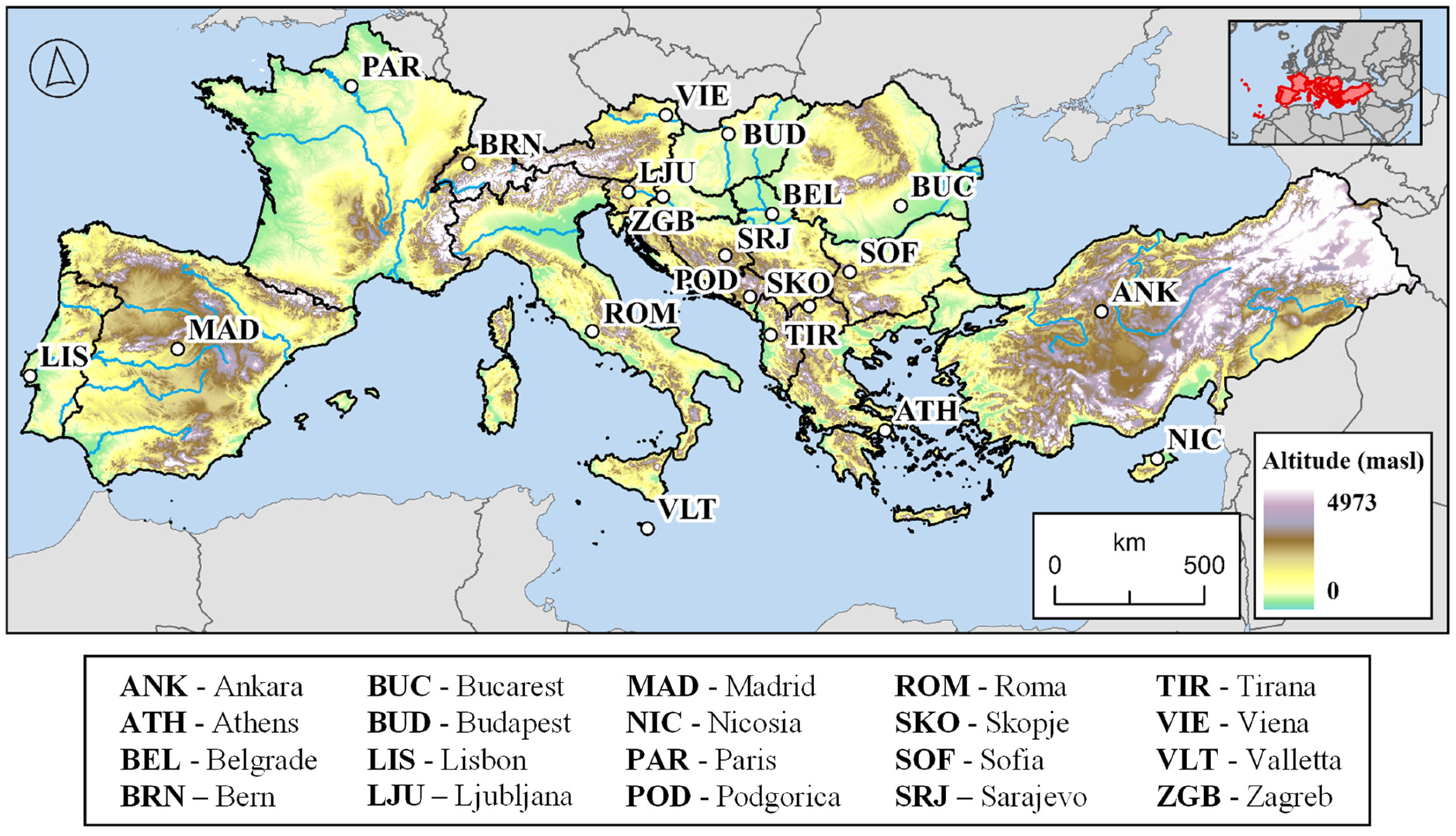
2.1. Study Area

The European Mediterranean Basin (or Euro-Med) is typically defined as the collection of river basins draining into the Mediterranean Sea. However, for the purposes of this research, countries within the region were considered in their entirety to provide comprehensive information in an area particularly vulnerable to climate variability (Figure 1). The selected study area, covering an area of over 3 million km², is delimited by the parallels 34°N and 52°N, and by the meridians −10°W and 45°E.

In terms of its topography, the area is notably mountainous due to the significant geological changes during the Alpine orogeny [72]. Prominent mountain systems include the Alps, north of the Italian Peninsula, and the Armenian Highlands, east of Turkey, with peaks exceeding 4800 m. Other relevant mountain ranges include the Sierra Nevada and the Pyrenees in Southeastern and Northwestern Spain, respectively; the Apennines in Central Italy; the Dinaric Alps along the Adriatic coast; the Carpathians in Romania; and the Balkans in Bulgaria. The major river basins in the region include the Danube, Rhône, and Po, which collect much of the Alpine water. The Ebro in Southeastern Spain and the Kizilirmak in Northern Turkey are also notable for their flow rates.

Regarding its climatology, much of the territory experiences pronounced seasonality in precipitation, resulting in a summer drought lasting for at least two consecutive months. These areas have a subtropical or Mediterranean climate, with average annual temperatures ranging from 18 to 24 °C and summer averages between 28 and 36 °C [21,73]. The northern zones north of the 45° parallel, however, have temperate climates, with a more stable hydrological regime, no summer drought, and milder temperatures throughout the year [21].

2.2. Data Collection

2.2.1. GCMs Temperature Data

Monthly mean temperature data simulated by 34 CMIP6 GCMs were obtained from the Lawrence Livermore National Laboratory node of the World Climate Research Program website (https://esgf-node.llnl.gov/projects/cmip6/, accessed on 16 December 2022). The GCMs selected, along with their supporter institution and their native resolution, are listed in

Table 1. The 34 CMIP6 Global Circulation Models (GCMs) selected in this study and their attributes (supporter institution, name, and native resolution).

Supporter Institution	GCM Name	Native Resolution (x, y)
Commonwealth Scientific and Industrial Research Organization (Australia)	ACCESS-CM2	1.875° × 1.250°
	ACCESS-ESM1-5
Canadian Centre for Climate Modelling and Analysis (Canada)	CanESM5	2.813° × 2.789°
	CanESM5-CanOE
Beijing Climate Center (China)	BCC-CSM2-MR	1.125° × 1.121°
	BCC-ESM1	2.813° × 2.789°
Chinese Academy of Meteorological Sciences (China)	CAMS-CSM1-0	1.125° × 1.121°
Nanjing University of Information Science and Technology (China)	NESM3	1.875° × 1.865°
Institute of Atmospheric Physics Chinese Academy of Sciences (China)	CAS-ESM2-0	1.406° × 1.417°
Institute of Atmospheric Physics, Chinese Academy of Sciences (China)	FGOALS-f3-L	1.250° × 1.000°
The First Institution of Oceanography (China)	FIO-ESM2-0	1.250° × 0.942°
Centre National de Recherches Météorologiques (France)	CNRM-CM6-1	1.406° × 1.400°
	CNRM-ESM2-1
Institut Pierre-Simon Laplace/Centre National de Recherche Scientifique (France)	IPSL-CM6A-LR	2.500° × 1.268°
	IPSL-CM6A-LR-INCA
Max-Planck-Institut fuer Meteorologie, Deutsches Klimarechenzentrum (Germany)	MPI-ESM1-2-HAM	1.875° × 1.865°
	MPI-ESM1-2-LR
	MPI-ESM1-2-HR	0.938° × 0.935°
Centro Euro-Mediterraneo sui Cambiamenti Climatici (Italy)	CMCC-ESM2	1.250° × 0.942°
Indian Institute of Tropical Meteorology (India)	IITM-ESM	1.875° × 1.904°
National Institute for Environmental Studies, Japan Agency for Marine–Earth Science and Technology (Japan)	MIROC6	1.406° × 1.400°
	MIROC-ES2L	2.813° × 2.789°
Meteorological Research Institute (Japan)	MRI-ESM2-0	1.125° × 1.121°
Bjerknes Centre for Climate Research, Norwegian Meteorological Institute (Norway)	NorESM2-MM	1.250° × 0.942°
Russian Academy of Sciences, Institute of Numerical Mathematics (Russia)	INM-CM5-0	2.000° × 1.500°
National Institute of Meteorological Sciences, Korea Met. Administration (South Korea)	KACE-1-0-G	1.875° × 1.250°
Korea Institute of Ocean Science and Technology (South Korea)	KIOST-ESM	1.875° × 1.895°
Met Office Hadley Centre (United Kingdom)	HadGEM-GC31-LL	1.875° × 1.250°
	UKES-M1-1-LL
National Center for Atmospheric Research	CESM2-WACCM	1.250° × 0.942°
Geophysical Fluid Dynamics Laboratory/NOAA (United States of America)	GFDL-ESM4	1.250° × 1.000 °
NASA Goddard Institute for Space Studies (United States of America)	GISS-E2-1-G	2.500° × 2.000°
	GISS-E2-2-G
University of Arizona—Department of Geosciences (United States of America)	MCM-UA-1-0	3.750° × 2.235°

. Only the first ensemble run (r1i1p1) was considered, shortening the timeframe to 1981–2010, which is the last 30-year period recommended by the World Meteorological Organization (WMO) and included in the CMIP6 historical experiment (1850–2014) [74].

2.2.2. ERA5 Land Temperature Data

ERA5 Land, the latest reanalysis product from the European Centre for Medium-Range Weather Forecasts (ECMWF), has emerged as one of the most widely utilized terrestrial reanalysis products to date [75].

Its remarkable simulation of in situ temperature is positioning it as the forefront product in the field. Several studies have reported a correlation exceeding r = 0.9 with observed temperatures, showcasing its exceptional ability to detect thermal fluctuations across various temporal scales (from intraday to intermonth) [76,77,78]. Moreover, it outperforms its predecessors in spatial resolution (0.1° $\approx$ 11.1 km) and simulation capacity [79,80], while also matching or surpassing satellite products. It has been suggested that, on a global scale, ERA5 Land is as proficient as satellite products like AIRS or MODIS in detecting temperature trends [81]. Furthermore, in regions characterized by complex topography, such as the Euro-Mediterranean region, ERA5 Land has been shown to outperform MODIS in trend detection while exhibiting less exaggeration of temperature increases [82]. Analogously, it has demonstrated greater accuracy in capturing both interdecadal and interannual temperature trends compared to NASA POWER, based on MERRA-2, and is more suitable for calculating specific extreme temperature indices [83].

While ERA5 has been used to evaluate the performance of GCMs land surface temperature simulation [84,85,86], our study would represent, to our understanding, the first use of ERA5 Land with that specific objective in mind. The monthly averaged temperature dataset from ERA5 Land was acquired through the Copernicus Climate Change Service (C3S) website (https://cds.climate.copernicus.eu/, accessed on 16 December 2022). The temporal window was adjusted, following the process conducted in the historical experiment of the GCMs, to the period 1981–2010.

2.3. Cross-Validation of Interpolation Methods

In this paper, GCMs are interpolated to ERA5 Land resolution (0.1°). While this may seem a fine resolution, GCMs have already been interpolated to this or lower scales [56,87,88]. Even downscales of less than one square kilometer have been performed [89]. Bilinear interpolation is undoubtedly the most commonly used method either when matching the spatial resolution of GCMs or when adjusting them to the reference dataset [32,35,52,56,87]. However, this may not be the optimal way to do it, and the data may be undergoing significant transformation. Therefore, it is intended to establish which interpolation method is the least data-modifying in a specific study area.

Six interpolation methods are tested in this paper: Bilinear Interpolation (BI), Inverse Distance Weighting (IDW), Kernel Smoothing (KS) and three Kriging methods: Ordinary Kriging (OK), Cokriging (plus Elevation) (COK+E) and Empirical Bayesian Kriging (EBK). The former two are deterministic methods, whereas Kriging is a geostatistical technique based on the methodical computation of the influence of certain points on other adjacent points [90]. On the other hand, Kernel is a polynomial method based on the obtention of the optimal prediction polynomial for each pixel [91].

The aforementioned interpolation methods were compared using a cross-validation procedure based on the error between raw data and the interpolated output [92,93]. It consists of a leave-one-out cross-validation, which is the default cross-validation procedure provided by the program in the version adopted. From the native resolution of each GCM, which is very divergent from each other, as shown in Table 1, we applied the aforementioned interpolation methods, setting 0.1° as the target (output) resolution. Spatial Analyst and Geostatistical Analyst extensions of ESRI ArcGIS 10.8 were used [94].

2.4. GCMs Performance Assessment and Ranking

An extensive review would be required to explain in detail the profusion of methods available for assessing and ranking General Circulation Models (GCMs): reliability ensemble averaging, relative entropy, symmetric uncertainty, Bayesian approaches, probability density functions, or clustering are merely a sample of this wide diversity [57]. Nevertheless, despite the multitude of existing methods, conventional metrics continue to be used in GCM evaluation, as they offer greater comparability across studies [57]. Furthermore, they vary within known ranges, making them easily interpretable. These conventional metrics, also referred to as goodness-of-fit (GOF) metrics, employ simple calculations to compare the values of GCMs with those of a reference dataset—in this case, ERA5 Land.

Coefficient of Correlation (CC), Normalized Root Mean Squared Error (NRMSE), Nash–Sutcliffe Efficiency (NSE), Kling–Gupta Efficiency (KGE), and modified index of agreement (md) were implemented as GOF metrics in this study. All of them were devised to assess various facets of two data distributions to ascertain whether both sets of data could stem from a shared underlying distribution. Indeed, this serves as one of the primary rationales underpinning the utilization of diverse goodness-of-fit metrics. Their mathematical formulas are provided below (Equations (1)–(5)).

$$CC=\frac{\sum _{i=1}^N({sim}_i-\overline{sim})({obs}_i-\overline{obs})}{\sqrt{\sum _{i=1}^N{({sim}_i-\overline{sim})}^2}·\sqrt{\sum _{i=1}^N{({sim}_i-\overline{sim})}^2}}$$

(1)

$$NRMSE=\frac{\sqrt{\frac{1}{N}\sum _{i=1}^N{({sim}_i-{obs}_i)}^2}}{{obs}_{\left(max\right)}-{obs}_{\left(min\right)}}$$

(2)

$$NSE=1-\frac{\sum _{i=1}^N{({sim}_i-{obs}_i)}^2}{\sum _{i=1}^N{({obs}_i-\overline{obs})}^2}$$

(3)

$$KGE=1-\sqrt{{\left(CC-1\right)}^2+{\left(\frac{\overline{sim}}{\overline{obs}}-1\right)}^2{\left(\frac{\raisebox{1ex}{${\sigma }_{sim}$}\!\left/ \!\raisebox{-1ex}{$\overline{sim}$}\right.}{\raisebox{1ex}{${\sigma }_{obs}$}\!\left/ \!\raisebox{-1ex}{$\overline{obs}$}\right.}-1\right)}^2}$$

(4)

$$md=1-\frac{\sum _{i=1}^N{\left|({obs}_i-{sim}_i)\right|}^j}{\sum _{i=1}^N \left|{sim}_i-\overline{obs}\right|+{\left|({obs}_i-\overline{obs})\right|}^j}$$

(5)

where ${sim}_i$ stands for simulated data, ${obs}_i$ for observed data, $\overline{sim}$ for mean simulated data, $\overline{obs}$ for mean observed data, ${\sigma }_{sim}$ for simulated data variance, ${\sigma }_{obs}$ for observed data variance, and N for the number of records.

All metrics presented, except for NRMSE, have a range that reaches its maximum at the value 1, representing the ideal fit between simulation and observation. The only difference is that both CC (Equation (1)) and md (Equation (5)) have a lower bound of 0, where this value represents total disagreement between simulation and observation, while NSE (Equation (3)) and KGE (Equation (4)) have no lower limit, so the closer a value is to −∞, the worse the model–reality relationship. On the other hand, NRMSE has the opposite interpretation: it varies between 0 and 1, with 0 representing the ideal fit and positive values representing the error between simulation and observation. Examples of the application of the GOF metrics can be found in current research [52,55,60,61,95].

Logically, from each of the GOF metrics, a ranking is obtained that orders the different GCMs from worst to best according to their value for that metric. To obtain an overall ranking, the most common approach is to resort to a method based on a single index, which most studies typically refer to as the Comprehensive Rating Index (CRI) [60,96,97]. Its mathematical expression is presented herein (Equation (6)).

$$CRI=1-\frac{1}{nm}\sum _{i=1}^n{Rank}_i$$

(6)

where n is the number of metrics (5); m is the number of models evaluated (34); and Rank_i represents the ranking position of GCM m based on metric n, ranging from 1 to 34. Hence, the closer the model is to CRI = 1, the better it fits ERA5 Land reanalyzed data.

2.5. Multi-Model Ensemble and Future Projections

Multi-Model Ensemble (MME) methods have been classified into unweighted and weighted [98]. Unweighted procedures have been recommended and employed as standard practice for several decades, primarily due to their ease of use [3]. The most widely used among these methods is the Simple Averages Multi-Model Ensemble (SAE). However, it has been found that weighted methods, especially those based on machine learning algorithms, produce better results and reduce the systematic biases inherent in each GCM [99,100]. Within these, the Random Forest Multi-Model Ensemble (RFE) has proven to be one of the most practical, accurate, and popular methods currently [100].

Both SAE and RFE were compared in this research. The SAE was obtained by directly averaging the values of the GCMs intended for ensemble. For a more detailed explanation of how to obtain an RFE, one should refer to the original publication [101]. However, it is worth mentioning that the parameters used were n_tree = 500, and m_try = 2, with 80% of the data for calibration, and the reanalyzed temperature was used as the independent variable.

To select the number of models included in the MME, the “best MME” criterion was followed. This involved generating 34 MMEs by adding the 34 GCMs in order of ranking and selecting the MME with the maximum correlation with the reanalyzed temperature. This approach is similar to that used by other authors [61]. However, as an innovation, this study also considers the “explained variance” criterion. This criterion entails determining which of the 34 designed MMEs predominantly explains (has a higher percentage of) the variance present in the ERA5 Land reference database. In other words, for instance, if the variance of ERA5 Land is 1.0, an MME with a variance value of 0.85 would be considered better, initially, than one with a value of 0.80.

Finally, the optimal MME obtained will be used to establish projections for short-term (2026–2050), medium-term (2051–2075), and long-term (2076–2100) periods under different greenhouse gas emission scenarios from CMIP6: optimistic (SSP1-RCP2.6), intermediate (SSP2-RCP4.5), and pessimistic (SSP5-RCP8.5) [102]. Emission scenarios data were also obtained from the Lawrence Livermore National Laboratory node of the World Climate Research Program website (https://esgf-node.llnl.gov/projects/cmip6/, accessed on 16 December 2022)

3. Results

3.1. Cross-Evaluation of Interpolation Methods

Six interpolation methods were applied to match the resolution of the 34 GCMs, with the resolution of the reference dataset being (0.1°): Inverse Distance Weighting (IDW), Bilinear Interpolation (BI), Kernel Smoothing (KS), Ordinary Kriging (OK), Cokriging plus Elevation (COK+E), and Empirical Bayesian Kriging (EBK). Figure 2 shows the Mean Error (ME) and Root Mean Square Error (RMSE) between GCM value in its native resolution and GCM value in its interpolated resolution (0.1°) for the 34 selected GCMs. Concerning the deterministic methods (BI and IDW), subtle discrepancies between them are noted, albeit both exhibiting similar downscaling capabilities, as indicated by their comparable RMSE values (0.9 versus 0.8 as the median value). BI manifests a ME range spanning from +0.08 to −0.013, with certain disregarded outliers reaching extremes of +0.18 and −0.35. Conversely, IDW displays a maximum ME of +0.02 and a minimum of −0.06. In general, IDW demonstrates greater stability as a deterministic method (with lesser intermodel discrepancies) than BI, with its median value in closer proximity to 0, and displaying either a slight or negligible propensity for underestimation. The polynomial KS method mirrors IDW’s traits, albeit exhibiting a substantially compressed median value around 0 and a diminished RMSE, with a median hovering around 0.6. Among geostatistical methods, EBK emerges as the exemplar, showcasing the lowest error values, both in terms of ME and RMSE. Its entire ME spectrum spans from +0.005 to −0.004, positioning it closest to 0, while registering scarce absolute under or overestimations. The median value of its RMSE stands at 0.41, unequivocally the most minimal. Conversely, neither KS nor COK+E yield favorable outcomes, yielding even poorer estimates than deterministic counterparts. Particularly, COK+E’s ME values exhibit a marked skew towards underestimation (median = −0.05), with standardized error values surpassing 1 for several GCMs, constituting their median. Although OK portrays a more acceptable ME range (−0.06 to +0.06, with outliers disregarded), it yields RMSE values similar to those of COK+E.

The outcomes regarding individual model deviations are illustrated in Figure 3. It is evident that EBK stands out as the method that minimizes RMSE to the greatest extent, with values equal to or less than 0.5 for the majority of GCMs. Even in models with certain “resistance” to interpolation, such as those from the IPSL and GISS families, along with KIOST, which consistently exhibit errors irrespective of the method employed, the application of EBK appears to mitigate these discrepancies. BI, KS, and to a lesser extent, IDW, also demonstrate considerable consistency. Conversely, both OK and COK+E display substantial errors, with values close to or exceeding 1.5 in RMSE for models from the CNRM, CMCC, and CESM2 families, and significant errors ranging between 1.0 and 1.5 in RMSE for numerous other GCMs (Hadley, MPI, or GFDL families), underscoring once again their inability to yield acceptable downscaling results.

Finally, it is imperative to underscore the geospatial disparities observed in the interpolation of each GCM. To illustrate this, a particular model, the HadGEM-GC31-LL, was chosen as an example, and its spatial distribution of errors in the Euro-Med region is delineated in Figure 4. Notably problematic areas arise across all methods except for EBK. These problematic zones are concentrated in Central and Eastern Turkey, as well as in high-altitude regions such as Northern Spain, Central France, the Alps, the Dinaric Alps, and the Balkans. In these areas, methods such as IDW, OK, and especially COK+E, alter the data by up to +4.4 °C. Additionally, a profound depression is observed in the center of the Czech Republic, where the alteration reaches as low as −4.2 °C. Although BI exhibits more consistency than the previous methods and does not manifest such gross positive errors (maximum of +3.5 °C), it demonstrates negative errors across virtually the entire study area, with areas of significant modification (exceeding −3.8 °C) in Eastern Spain, Southern Turkey, or the Franco-Italian coast.

Regarding EBK, it shows its greatest strength in these findings, as the low error rate (Figure 2) and consistency among models observed previously (Figure 3) translate into remarkable spatial regularity. The entire range of data alteration through interpolation ranges from −1.15 °C (Czech Republic) to +1.41 °C (Eastern Turkey), significantly lower than that of any other method. However, despite specific zones, such as in most of the territory, the range of modification oscillates between +0.19 and +0.35 °C.

The superiority of EBK as the interpolation method with the least data modification was demonstrated on the global error rate, intermodel consistency, and geospatial regularity level. Therefore, this Bayesian approach is implemented to equalize the scale of the 34 selected GCMs to that of the ERA5 Land reference dataset (0.1°).

3.2. Ranking and Assessment of GCMs

Table 2. Goodness-of-fit between General Circulation Models (GCMs) and ERA5 Land temperature data. NRMSE, Normalized Root Mean Squared Error; NSE, Nash–Sutcliffe Efficiency; KGE, Kling–Gupta Efficiency; CC, Correlation Coefficient; md, modified index of agreement. Comprehensive rating index (CRI) value and overall rank are also displayed. The rank for each metric is shown between brackets. The top 5 models for each variable are highlighted in bold.

GCM	NRMSE (%)	NSE	KGE	CC	md	CRI
ACCESS-CM2	53.20 (16)	0.72 (16)	0.85 (5)	0.87 (20)	0.75 (14)	0.58 (14)
ACCESS-ESM1-5	57.60 (22)	0.67 (22)	0.72 (28)	0.86 (23)	0.72 (20)	0.32 (24)
BCC-CSM2-MR	49.30 (12)	0.76 (12)	0.80 (13)	0.87 (21)	0.77 (11)	0.59 (11)
BCC-ESM1	66.60 (30)	0.56 (30)	0.65 (32)	0.77 (32)	0.67 (30)	0.09 (31)
CAMS-CSM1-0	51.70 (14)	0.73 (14)	0.82 (12)	0.90 (10)	0.73 (19)	0.59 (12)
CanESM5	58.70 (26)	0.66 (26)	0.75 (25)	0.83 (28)	0.72 (23)	0.25 (28)
CanESM5-CanOE	58.20 (24)	0.66 (24)	0.76 (22)	0.83 (29)	0.72 (21)	0.29 (26)
CAS-ESM2-0	57.70 (23)	0.67 (23)	0.77 (20)	0.91 (8)	0.71 (25)	0.42 (20)
CESM2-WACCM	57.40 (21)	0.67 (21)	0.75 (26)	0.91 (5)	0.71 (24)	0.43 (19)
CMCC-ESM2	55.60 (19)	0.69 (19)	0.78 (17)	0.89 (13)	0.73 (17)	0.50 (17)
CNRM-CM6-1	41.70 (3)	0.83 (3)	0.87 (3)	0.91 (4)	0.80 (3)	0.91 (3)
CNRM-ESM2-1	44.40 (7)	0.80 (7)	0.86 (4)	0.91 (7)	0.78 (7)	0.81 (5)
FGOALS-F3-L	47.80 (9)	0.77 (9)	0.74 (27)	0.89 (14)	0.76 (12)	0.58 (15)
FIO-ESM2	59.20 (27)	0.65 (27)	0.77 (21)	0.90 (9)	0.70 (28)	0.34 (23)
GFDL-ESM4	42.40 (4)	0.82 (4)	0.89 (1)	0.94 (1)	0.80 (4)	0.92 (2)
GISS-E2-1-G	46.90 (8)	0.78 (8)	0.78 (15)	0.89 (15)	0.77 (10)	0.67 (10)
GISS-E2-2-G	73.60 (31)	0.46 (31)	0.72 (29)	0.88 (17)	0.61 (32)	0.18 (29)
HadGEM-GC31-LL	48.00 (11)	0.77 (11)	0.84 (6)	0.88 (16)	0.77 (9)	0.69 (8)
IITM-ESM	57.10 (20)	0.67 (20)	0.83 (10)	0.84 (26)	0.73 (18)	0.45 (18)
INM-CM5-0	62.90 (29)	0.60 (29)	0.68 (31)	0.83 (30)	0.70 (26)	0.15 (30)
IPSL-CM6A	44.30 (6)	0.80 (6)	0.84 (7)	0.90 (11)	0.79 (6)	0.79 (6)
IPSL-CM6A-INCA	44.10 (5)	0.81 (5)	0.83 (9)	0.90 (12)	0.79 (5)	0.79 (7)
KACE-1-0-G	51.70 (13)	0.73 (13)	0.78 (18)	0.87 (22)	0.75 (13)	0.54 (16)
KIOST-ESM	60.00 (28)	0.64 (28)	0.78 (16)	0.88 (19)	0.69 (29)	0.29 (27)
MCM-UA-1-0	76.00 (32)	0.42 (32)	0.51 (34)	0.69 (34)	0.59 (33)	0.03 (34)
MIROC6	90.90 (34)	0.17 (34)	0.68 (30)	0.80 (31)	0.58 (34)	0.04 (32)
MIROC-ES2L	78.60 (33)	0.38 (33)	0.61 (33)	0.71 (33)	0.64 (31)	0.04 (33)
MPI-ESM1-2-HAM	58.60 (25)	0.66 (25)	0.79 (14)	0.85 (24)	0.70 (27)	0.32 (25)
MPI-ESM1-2-HR	41.00 (2)	0.83 (2)	0.88 (2)	0.92 (3)	0.82 (1)	0.94 (1)
MPI-ESM1-2-LR	54.20 (17)	0.71 (17)	0.76 (24)	0.85 (25)	0.74 (16)	0.42 (21)
MRI-ESM2-0	40.20 (1)	0.84 (1)	0.83 (11)	0.92 (2)	0.81 (2)	0.90 (4)
NESM3	55.50 (18)	0.69 (18)	0.76 (23)	0.83 (27)	0.72 (22)	0.36 (22)
NorESM2-MM	52.90 (15)	0.72 (15)	0.77 (19)	0.91 (6)	0.74 (15)	0.59 (13)
UKES-M1-1-LL	47.90 (10)	0.77 (10)	0.83 (8)	0.88 (18)	0.78 (8)	0.68 (9)

presents the performance of each of the 34 GCMs for each of the five GOF metrics used. These results stem from a pixel-to-pixel comparison of the annual mean temperature at 0.1° provided by each interpolated GCM versus the observed (reanalyzed) by ERA5 Land. Additionally, the table displays the global ranking based on the Comprehensive Rating Index (CRI).

Regarding the GOF metrics, both NRMSE and NSE offer identical rankings. They appear to be the ones that show the greatest range of variability among models, as they oscillate, from worst to best GCM, between 90.9 and 40.2 for NRMSE (%) and between 0.17 and 0.84 for NSE. It is noteworthy that NSE does not exhibit negative values, ensuring that no GCM presents an aberrant temperature simulation. Conversely, CC seems to provide the least information, as its interquartile range of values ranges from 0.85 to 0.89, with only three models below 0.8. It could be attributed to the data distribution of the GCMs and to the intrinsic characteristic of the metric. It could be hypothesized that in coarse-resolution models, the inner variance is small and therefore the difference between the simulated value of a pixel and the mean value is minimal. In these particular cases, metrics like CC virtually measure the observed variance of the data distribution, resulting in similar CC values for almost all models. On the other hand, metrics such as NRMSE or NSE compare (subtract) the simulated and observed data distributions, yielding results with a wider range of values. Moreover, models with a high correlation with the reanalyzed temperature can be identified, but their data distribution, according to the other metrics, is significantly distant from the reanalyzed data. For instance, CESM2-WACCM exhibits a correlation with ERA5 Land exceeding 0.9, ranking 5th for this metric, yet occupying a position below 20th for the rest of the metrics. CAS-ESM2-0, FIO-ESM2, or NorESM2-MM present a similar problem.

Concerning the models, none repeat the same ranking position for the five analyzed metrics. Models from the CNRM family and MIROC-ES2L exhibit the most repetitions: CNRM-CM6-1 ranks 3rd on four occasions, CNRM-ESM2-1 occupies the 7th position on four occasions, and MIROC-ES2L is placed 33rd on four occasions. GFDL-ESM4 (4th), MPI-ESM1-2-HR (2nd), MIROC6 (34th), BCC-ESM1 (30th), and IPSL-CM6A (6th) also show consistency in their results and repeat their ranking position at least three times without significant fluctuations or performance losses.

Lastly, regarding the CRI value, the top five models demonstrating overall superior performance, from highest to lowest, are MPI-ESM1-2-HR, GFDL-ESM4, CNRM-CM6-1, MRI-ESM2-0, and CNRM-ESM2-1. Models from the IPSL and Hadley families, along with GISS-E2-1-G, complete the top 10.

3.3. Geospatial Performance Analysis

The aforementioned pixel-by-pixel comparison of model performance, which reveals the geospatial component of this variable, is the main advantage of the developed method. In other words, it allows for the identification of areas where GCM-simulated temperatures are close to those reanalyzed by ERA5 Land, as well as areas where this simulation capacity decreases drastically. To our knowledge, our study is the first to propose a geospatial context for the CRI value, which has previously only been used to rank models based on their overall performance across multiple metrics.

Figure 5 confirms that models do not behave uniformly across the Euro-Med region. The MPI-ESM1-2-HR, which proved to be the most competent, shows areas of decreasing temperature simulation, such as the central regions of Spain and France or the Black Sea coast (Eastern Romania and Bulgaria). Conversely, it is the best at simulating temperatures in high altitude areas, which is remarkable in such a rugged region. Its CRI values are equal to or close to 1 in the Alps, the Dinaric Alps, and the entire Turkish plateau, and very high (0.8–1.0) in the Apennines (Italy) or the Sierra Nevada (Spain). Interestingly, the two models in the CNRM family show similar patterns, although both have deeper dips in performance, particularly the CNRM-ESM2-1, whose CRI values range from 0.15 to 0.40 in Northwest France and the Black Sea Coast. The GFDL-ESM4 and MRI-ESM2-0 models appear to be much more regular among those with competent simulations, as they do not show areas where the simulation drops drastically. The use of GFDL-ESM4 appears to be preferable in Northwest and Southeast Spain and Northern Turkey, while MRI-ESM2-0 appears to simulate exceptionally well along the entire Adriatic and Black Sea coasts, precisely where other better-ranked models fail miserably.

Other models showing poorer overall performance but whose use may be locally justified include: (i) HadGEM-GC31-LL in Northwestern France, (ii) GISS-E2-1-G on the coast of the Black Sea (and in Northwestern France), (iii) UKES-M1-1-LL in the Aegean Sea, and (iv) IPSL models in Central Europe. Regarding the latter, especially in the case of IPSL that does not include the atmospheric chemistry/aerosol microphysics model (INCA), it should be noted that they competently model the Atlantic/temperate zones of the study area but seem to lose capacity in the large Mediterranean/subtropical zones such as the Iberian Peninsula, Italy, Greece, or Eastern Turkey.

Finally, among the models that simulate the temperature in the Euro-Mediterranean region poorly, MCM-UA-1-0, MIROC-ES2L and MIROC6 are clearly the worst performers, with CRI values below 0.25 in almost all points of the region. BCC-ESM1, GISS-E2-2G, INM-CM5-0, NESM3, or the MPI version with the Hamburg Aerosol Model (HAM) also show a globalized low CRI value. However, our analysis corroborates that even these GCMs can have local simulation peaks in certain areas. For instance, BCC-ESM1 correctly reproduces temperatures in Eastern Romania, MPI-ESM1-2-HAM in the Bulgarian Balkans, and INM-CM5 in Hungary and Northern Serbia. Therefore, even GCMs that are considered “disposable” due to their poor overall performance can be used in certain sub-regions as viable alternatives to models with better overall simulation, or as entities to be included in a Multi-Model Ensemble to improve the capture of existing climate variability.

3.4. Multi-Model Ensemble

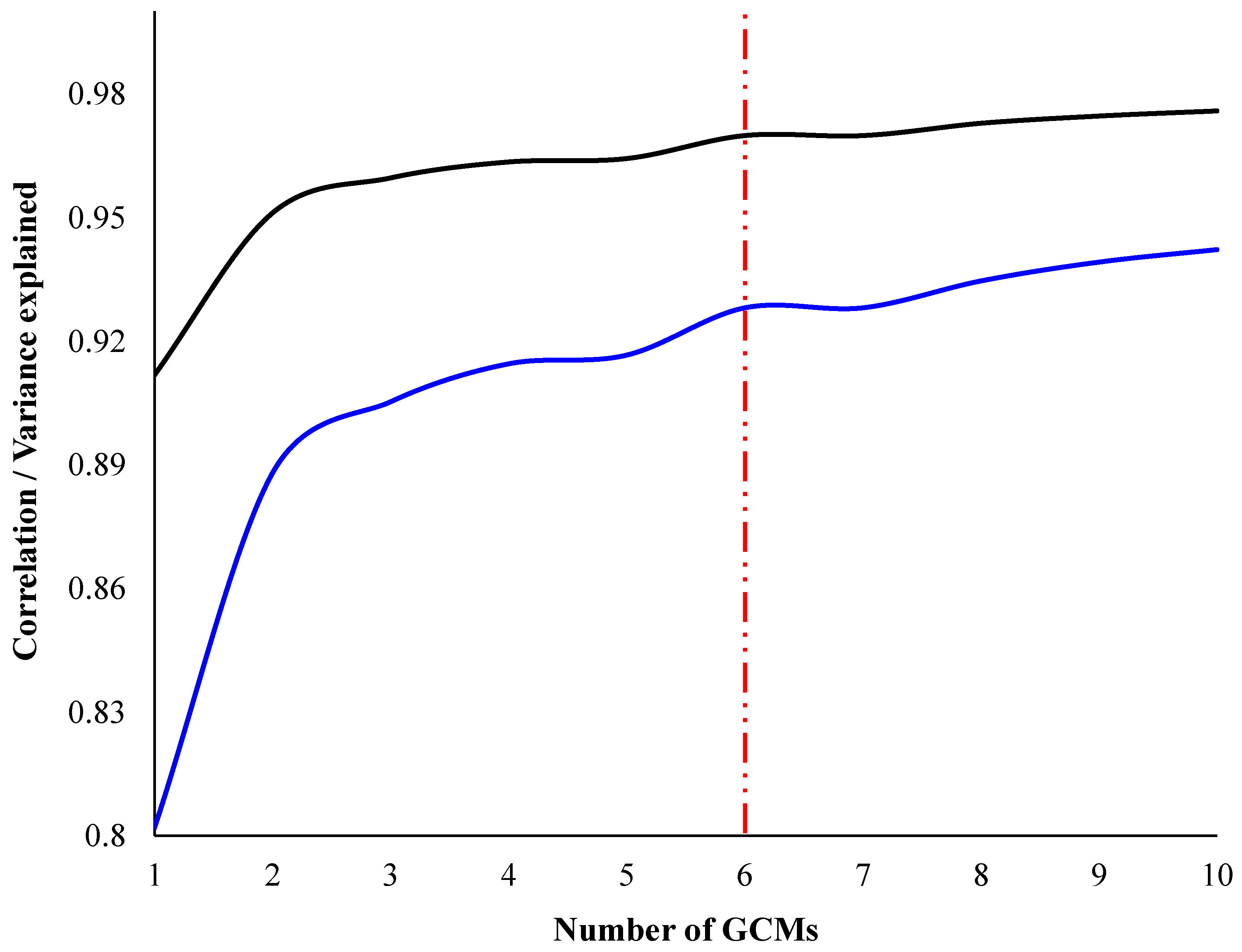
3.4.1. Determining Ensemble Members

Figure 6 illustrates the correlation and explained variance as a function of the number of additional models added, in strict order of the ranking obtained in Table 2, to the Multi-Model Ensemble (MME). It is evident that with an increasing number of added GCMs, the ensemble value becomes closer to the value of ERA5 Land, resulting in an increase in both correlation and explained variance. With just one GCM (MPI-ESM1-2-HR), the correlation already exceeds 0.9, and the explained variance is greater than 0.8. With three GCMs (MPI-ESM1-2-HR + CNRM-CM6-1 + GFDL-ESM4) the variance explained is greater than 0.9 and the correlation value rises to 0.96. Although at three GCMs the MME has already improved considerably, a slight but constant increase is observed until the value of six GCMs is reached (0.97 in correlation and 0.93 of explained variance). From this value onwards, neither the correlation nor the explained variance improves significantly. Hence, the number of GCMs considered for MME is six GCMs: MPI-ESM1-2-HR, CNRM-CM6-1, GFDL-ESM4, CNRM-ESM2-1, MRI-ESM2-0, and IPSL-CM6A-LR.

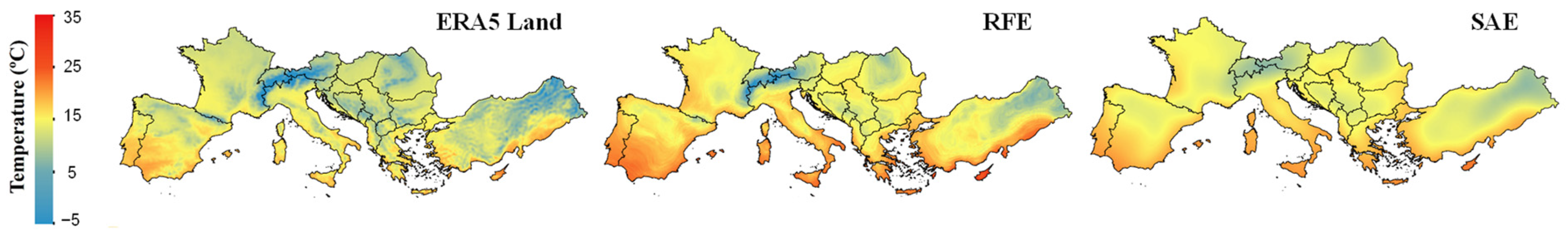
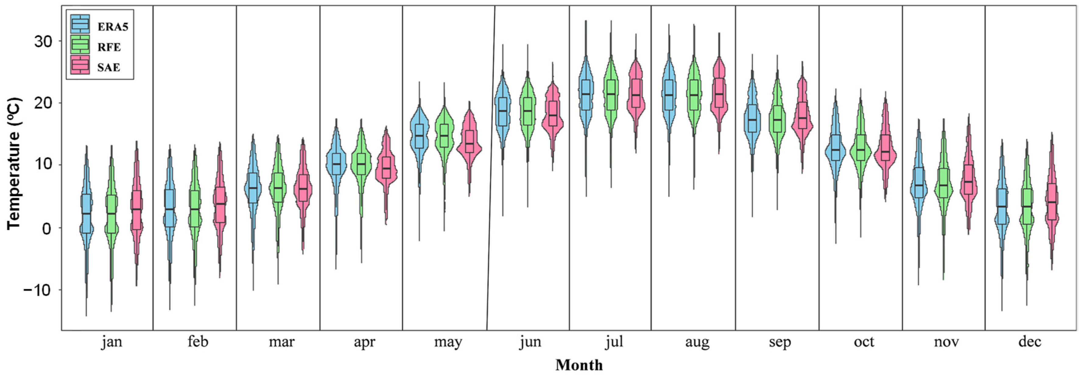
3.4.2. Simple Averages vs. Random Forest Multi-Model Ensemble

Figure 7 shows how the Random Forest Multi-Model Ensemble (RFE) exhibits significantly improved accuracy in capturing temperature patterns of ERA5 Land on an annual basis, but for a slight overestimation tendency in the southern half of the Iberian Peninsula, the coast of Sardinia, Italy, Southern Turkey, and Cyprus. Having said that, RFE accurately depict the temperatures in the higher foothills of the study area, especially in the Alps, the Carpathians, and the Armenian System. Conversely, Simple Averages Multi-Model Ensemble (SAE), clearly attenuates the contrasts between the coldest and warmest regions, resulting in the loss of extreme values. The RFE superiority in reproducing the observed (reanalyzed) temperature can also be observed at the monthly scale. In this regard, Figure 8 demonstrates that a proper simulation of monthly temperature can be achieved through an annual-scale evaluation of the GCMs that perform best for a specific study area. It can be observed that the RFE not only captures the temperature range of ERA5 Land perfectly for each month but also reproduces an almost identical distribution and provides appropriate detection of extreme values (whiskers of the diagram). In contrast, the SAE tends to overestimate central values and shows a significant inability to capture extreme values. Particularly, it is less effective in detecting the lowest temperatures of each month, as clearly observed during the months of December, April, May, June, September, and October.

Finally, Figure 9 illustrates the correlation between the percentage importance assigned by the regression method used in the RFE and the CRI value obtained in the ranking (Table 2). Although a positive correlation detected between these variables (Rho = 0.23), it is not statistically significant (p > 0.05). Thus, it is observed that when performing an RFE with the total pool of analyzed GCMs, the regression method automatically discards several of them (GISS-E2-1-G, MPI-ESM1-2-LR, NESM3, etc.) by assigning them 0% importance. However, it also includes, although with little overall importance, models considered as “poor performers” (BCC-ESM1, MIROC6, and MIRPC-ES2L). At the same time, it discards “good performers” (IPSL models, HadGEM-GC31-LL, and UKES-M1-1-LL). In conclusion, we could argue that the majority of the assigned importance is distributed among three of the GCMs that performed best in the ranking: GFDL-ESM4 (14%), MRI-ESM2-0 (6%), and MPI-ESM1-2-HR (3%).

3.5. Future Temperature Projections

In this section, future projections regarding mean seasonal and annual temperature in the Euro-Med region for the short-term (2026–2050), medium-term (2051–2075), and long-term (2076–2100) periods, based on different emission scenarios (SSP1-RCP2.6, SSP2-RCP4.5, and SSP5-RCP8.5), will be established using the previously developed MME. The projections obtained in this study will be contextualized according to the predictions of the IPCC at both global and regional (Euro-Med) scales. The confidence intervals provided by the IPCC were obtained from the Interactive Atlas developed by the Working Group I for AR6 [103], and they are documented in

Table A1. Ranges of annual and seasonal temperature increase expected by the IPCC at the global level (GL) and for the Euro-Med (MED) region under different emission scenarios (SSP1-RCP2.5, SSP2-RCP4.5, and SSP5-RCP8.5) in the short (2026–2050), medium (2051–2075), and long (2016–2100) term. Information obtained from the IPCC WGI Interactive Atlas [103].

		SSP1-RCP2.6			SSP2-RCP4.5			SSP5-RCP8.5
		Short	Medium	Long	Short	Medium	Long	Short	Medium	Long
Annual	GL	0.8–1.2	1.0–2.6	0.9–2.6	0.8–1.2	1.2–1.7	1.8–2.6	0.9–1.2	1.6–2.2	3.3–4.9
	MED	1.0–1.5	1.3–1.9	1.3–2.0	1.3–1.4	1.6–2.1	2.3–3.1	1.4–1.7	2.1–2.7	4.1–5.8
Winter (DJF)	GL	0.8–1.2	1.0–1.6	1.0–1.7	0.8–1.1	1.3–1.8	1.9–2.7	0.9–1.3	1.6–2.3	3.5–5.1
	MED	0.8–1.3	1.0–1.8	1.1–1.8	0.9–1.3	1.3–1.7	1.9–2.9	0.9–1.4	1.6–2.4	3.4–4.9
Spring (MAM)	GL	0.7–1.1	0.9–1.5	0.9–1.6	0.8–1.0	1.1–1.6	1.7–2.5	0.8–1.1	1.5–2.1	3.1–4.7
	MED	0.8–1.3	1.1–1.8	1.2–1.9	1.0–1.4	1.4–1.9	2.0–2.8	0.9–1.6	1.7–2.5	3.7–5.0
Summer (JJA)	GL	0.8–1.1	0.9–1.5	0.9–1.7	0.8–1.1	1.1–1.7	1.7–2.7	0.9–1.2	1.5–2.2	3.2–4.9
	MED	1.3–1.9	1.6–2.4	1.6–2.4	1.4–1.8	1.9–2.7	3.0–3.9	1.5–2.6	2.7–3.4	5.3–6.9
Autumn (SON)	GL	0.8–1.2	1.0–1.6	1.0–1.7	0.8–1.1	1.3–1.8	1.8–2.7	0.9–1.3	1.6–2.3	3.4–5.0
	MED	1.1–1.6	1.3–2.0	1.3–2.0	1.1–1.6	1.6–2.3	2.3–3.5	1.2–1.8	2.2–3.0	4.3–6.2

of Appendix A. The percentage of territory whose expected warming falls within the IPCC interval for each scenario and time window is presented in

Table A2. Percentage of agreement between the temperature anomalies identified in this study and those predicted by the IPCC [103] for the three analyzed emission scenarios (SSP1-RCP2.5, SSP2-RCP4.5, and SSP5-RCP8.5) and temporal periods (short, 2026–2050; medium, 2051–2075; and long, 2076–2100) at both annual and seasonal scales.

	SSP1-RCP2.6			SSP2-RCP4.5			SSP5-RCP8.5
	Short	Medium	Long	Short	Medium	Long	Short	Medium	Long
Annual	35.00	59.55	60.20	29.77	40.57	52.55	39.76	32.92	66.43
Winter (DJF)	20.44	33.22	33.29	14.33	21.40	20.40	20.02	28.11	5.26
Spring (MAM)	17.93	24.70	22.83	18.34	24.77	26.21	25.41	35.53	44.77
Summer (JJA)	30.56	48.19	51.04	31.24	46.74	64.42	57.49	39.36	71.92
Autumn (SON)	31.50	36.10	39.98	25.54	34.53	60.31	29.40	32.69	71.95

of Appendix A.

Figure 10 shows the seasonal results in the most optimistic scenario: SSP1-RCP2.6 (sustainability or “green road”). As observed, significant differences exist between the outcomes obtained in our study and those predicted by the IPCC at a global or regional scale. The percentage of study area whose increments align with these predictions is lower in winter and spring. In winter, only 20.4% of the study area falls within the interval expected by the IPCC in the short term, a value that expands to 33.4% in the long term. Overall, there is a more significant warming than expected by the IPCC. The areas where this detected warming is most intense (more than 2 °C with respect to the reference interval) correspond to those regions of higher elevation in the Euro-Mediterranean region, as well as the Mediterranean archipelagos. In the Central European plateau, the expected increase is also higher (0–+1 °C) than the global and regional average of the IPCC. In the case of spring, the agreement shown with respect to official predictions is even lower, as it stands at 17.9% in the short term and only increases to 22.8% in the long term. However, in this case, the official projections suggest that the warming will be much greater than that detected in this study, as most of the study area shows an increase between 0 and 2 °C lower than predicted by the IPCC. The Iberian plateau, the entire France, the Po basin (Italy), and large areas of Central Turkey are the main points where this pattern is detected. However, the elevated mountain systems continue to warm more than expected. The wide ranges offered by the IPCC for summer and autumn mean that much of the territory falls within them. In the long term, the agreement is over 51.4% in summer and 39.9% in autumn. In both seasons, except for the aforementioned areas, which are resistant to warming in any season and time period, the pattern indicates a warming greater than expected. Particularly noteworthy, in the case of summer, is that much of the Northwestern French territory expects a warming between 0 and 1 °C higher than expected by the IPCC.

Figure 11 depicts the results obtained for the intermediate emission scenario: SSP2-RCP4.5 (“middle of the road”). The patterns and trends are very similar to those discussed in the previous scenario. In winter, however, it is observed that in the short term, most of the region warms more than predicted by the IPCC (concordance of 14.3%). These areas of increase not exceeding 1 °C with respect to the official projections extend to the Portuguese Coast and much of France and Central Europe. However, this pattern seems to reverse over time, as in the long term, the concordance is close to 20%, but due to a reluctance to warm up as much as the IPCC prediction expects (1.8–3.1 °C between the global and regional predictions). However, much of France is close to these values, with an approximate average anomaly of +1.6 °C. In the other seasons, no different patterns are observed compared to those discussed for the pessimistic scenario, although it should be noted that, in the long term, the concordance for summer and autumn is 64.4% and 60.3%, respectively, with respect to the established interval.

Figure 12 presents the results for the pessimistic scenario: SSP5-RCP8.5 (fossil-fuel development or “highway”). Regarding winter, although in the short and medium term the results are similar to those of less pessimistic scenarios, in the long term, it is observed that only a small part of the Mediterranean region will warm as much as expected by the IPCC. The concordance obtained with this interval is 5.2%. Although most of the anomalies detected are positive, they do not reach the +4.1 °C increase, the lower limit of the reference interval. In this regard, we can classify the IPCC projections as more pessimistic than those obtained through our methodical application of a regional assessment with downscaling. Regarding summer and autumn, there is a noticeable accelerated increase in both cases in the medium term. In the case of summer, the Adriatic coast and much of Eastern Europe will warm by 2 °C above expectations, while other areas of Central Europe or the northwest half of France will warm by over 1 °C compared to the reference. This is particularly concerning because the upper reference limits for summer and autumn are +3.4 °C and over +3.0 °C, respectively, meaning that much of the region could experience increases exceeding +5.0 °C in seasonal average temperature anomalies from the mid-century onwards. In the long term, however, the consequent increase in the upper reference limit to +6.9 °C (summer) and +6.2 °C (autumn) results in a 71.9% concordance for both seasons. However, the Central–Eastern European region continues to experience intense summer overheating.

Finally, Figure 13 shows the analysis of annual temperature anomalies for the three emission scenarios in the short, medium, and long term. In the long term, the agreement with the IPCC percentages is quite high for all three scenarios: 60.2%, 52.6%, and 66.4% for the optimistic, intermediate, and pessimistic scenarios, respectively. The intermediate scenario SSP2-RCP4.5 shows the greatest discordance with the results obtained in this study. In the medium-to-long term, except for the Iberian Peninsula, Italy, and Central–Eastern Europe, as well as in the higher mountain systems where the detected anomaly is positive, temperature increases are rarely as significant as those predicted by the IPCC. The agreement is also low (32.9%) for the SSP5-RCP8.5 scenario in the medium term, likely influenced by the strong increase in summer mean temperatures detected. In this case, areas with an increase exceeding 2 °C compared to the reference could face a further increase of +4.7 °C in annual mean temperatures from mid-century onwards, which would rise to 4.9–5.8 °C by the end of the century.

In conclusion, the results analyzed indicate a clear warming signal in the Euro-Med region. However, the detailed assessment based on downscaling and ranking of models that perform best for the study area reveals certain local differences that diverge, in some cases, greatly from the global and regional predictions established by the IPCC.

4. Discussion

4.1. Downscaling of GCMs Temperature Data

Empirical Bayesian Kriging (EBK) has clearly yielded the best results and introduces the least modifications between raw and interpolated data. The superiority of this method over other interpolation methods has been highlighted in numerous instances in current scientific literature [104,105,106]. This may be attributed to its less restrictive assumptions regarding data distribution [107]. Bilinear interpolation (BI), although the most commonly used method for downscaling GCMs [32,35,52,56,87], did not yield positive results in our evaluation. This may be because, being a deterministic method, it applies uniformly across all regions of the territory, which may work against it in rugged areas such as the Euro-Med. The use of Inverse Distance Weighting (IDW), another deterministic and simple method, appears preferable, despite overestimation and unfavorable previous results [108,109], at least in the case of temperature in mountainous regions, in the absence of complex geostatistical methods like EBK. Regarding deficiencies in the interpolation of certain GCMs, a clear reason has not been identified. The native resolution of the models could be a possible cause. The internal structure and distribution of the data are more feasible possibilities, as they would explain why models of the same family manifest comparable errors.

Our study underscores the imperative for a thorough and meticulous examination of interpolation techniques that minimize errors when downscaling GCMs. Systematically defaulting to bilinear interpolation may substantially distort the values furnished by GCMs.

4.2. Ranking, Assessment and Ensemble of GCMs

In relation to the goodness-of-fit (GOF) metrics employed, it is noteworthy that both the low variability in the correlation coefficient values and the relative inconsistency shown in the rankings obtained for each measure were detected in several previous studies worldwide [53,61,110,111].

Regarding the GCMs, MPI-ESM1-2-HR (1st) was classified as the best overall performer in our study. Its predecessors (e.g., ECHAM4 and ECHAM5) were highlighted for their superior simulation of climatic variables in Europe, especially along the French coast and the northwest of the Iberian Peninsula [112]. Studies conducted in Southern Italy (Calabria and Sicily) or in Turkey also underscore this accurate temperature modeling [59,60]. Precisely in Southern Italy, the CRI detected in our study exceeds 0.85. However, only the high-resolution (HR) version exhibits such efficacy, as the medium–low-resolution versions (LR and HAM) rank 21st and 25th, respectively. The improvement of the Max Planck family models with increased resolution has been noted in other studies [40,60]. Additionally, studies that do not incorporate this high-resolution version do not highlight MPI or its derivatives as good simulators [58,113].

The MRI-ESM2-0 (fourth) is another model highlighted in our study. However, it is a controversial model since its previous versions were considered incapable of simulating European climate patterns [114]. Recent studies, however, place the CMIP6 version of MRI as one of the best performers in the Mediterranean [60,115]. Regarding other models that have demonstrated great simulation in our analysis, CNRM models (third and fifth) had already shown their superiority over IPSL models (sixth and seventh) ([40]), despite the significant improvement evidenced by the latter compared to their CMIP5 versions [41]. Some studies highlight IPSL models as good predictors of future extreme temperature scenarios in Southern Spain [58] or in simulating temperature in Italy [59]. On the other hand, Regional Circulation Models (RCMs) based on CNRM models had already been highlighted for their good simulation in Mediterranean locations such as the Segura River Basin (Spain) [113], Turkey [60], and Southern Italy [59]. Specifically, in the latter, the CRI detected by our work for the CNRM-ESM2-1 model exceeds 0.9, with CNRM-CM6-1 showing similar values. Some of these studies also highlight RCMs based on the EC-Earth model, which were not evaluated in our study due to sharing the same climatic component as ERA5 Land [40].

It is noteworthy that, despite the intermediate performance detected in our study, the Hadley Centre models (HadGEM-GC31-LL, eighth; UKES-M1-1-LL, ninth) or their predecessors have been recommended in numerous studies for their excellent simulation of atmospheric circulation and climate types in Europe [40,60,114,116,117,118]. Some studies even suggest that they outperform ECHAM/MPI models in some territories, such as the Catalan–Provençal coast, the Balkans, or Central Europe [112], a fact not observed in light of our results. However, many of these studies highlight their good reproduction of precipitation, focusing less on the accurate simulation of temperature detected in our research.

Some research has also pointed towards the good temperature simulation of the ACCESS1-0 model in the south of the Iberian Peninsula [58]. In our study, the performance of ACCESS-CM2 (14th) on the Southern and Eastern Spanish Coast is noteworthy (Figure 8), which is consistent with these previous results. The NorESM2-MM (13th) and FGOALS-f3-L (15th) models were not highlighted in our study. However, they show good performance in the south and east of Turkey, a fact highlighted in more local studies [60,61].

Regarding GCMs with poor performance, the MIROC models (32nd and 33rd) are unfortunately the most prominent in this regard. Studies using their previous versions had highlighted them as good predictors in the North Atlantic [114]. However, this study corrected Sea Level Pressure values before evaluating the models, whereas it is now considered that correcting GCM errors should never be performed before evaluation [87,119]. Recent studies implicitly discourage the use of MIROC models in the European region [118]. Their poor performance in the Eastern Mediterranean has also been previously detected [60]. On the other hand, the BCC models, especially the low-resolution version (BCC-ESM1) (31st), are also among the poor performers. Their poor performance had already been detected in other Mediterranean locations [58].

It is also noteworthy that none of the versions of the models that include aerosol sub-models (MPI-ESM1-2-HAM [71]), atmospheric chemistry (IPSL-CM6A-INCA [120]), or ocean circulation (CanESM5-CanOE [70]) perform better than the same versions that do not include these “improvements”.

Finally, regarding the Multi-Model Ensemble (MME), it is imperative to underscore the recognized superiority of the Random Forest Multi-Model Ensemble (RFE) over the Simple Averages method (SAE), as well as over Bayesian or machine learning-based approaches, as delineated in prior scholarly investigations ([100,111,121,122]). Furthermore, it merits mention that our study opted for a cohort of six models, a choice aligned with the guidance provided by antecedent research [111]. Nevertheless, the determination of an optimal ensemble size remains a subject of contention within the scientific discourse. While some scholars advocate for the adequacy of a mere three GCMs [123], others contend that a minimum of 25 GCMs is requisite to attain minimal error reduction [98]. It is pertinent to highlight that, in our study, even with two or three GCMs, the correlation and explained variance were deemed satisfactory (>0.9) (Figure 6). The proficient replication of temperature patterns across both annual and monthly timescales by our RFE underscores that exhaustive minimization of error may not be imperative; rather, identifying a suitable local minimum suffices. Additionally, it elucidates the intrinsic linkage between performance at extended temporal scales (annual) and shorter ones (monthly), a conjecture previously posited [62]. Thus, the execution of assessments and ensembles at protracted scales emerges as a pragmatic approach, entailing reduced computational demand and greater expediency under specific circumstances.

4.3. The Sizzling Future of the Euro-Med

Our study highlights certain deviations between the predictions made by the IPCC and those obtained through optimal downscaling, GCM evaluation, and subsequent elimination of inaccurate models (Figure 10, Figure 11, Figure 12 and Figure 13). Despite the scientific consensus on global warming, criticism and skepticism regarding the models or scenarios employed by the IPCC have continued to grow [124,125]. Some suggest that emission pathways may be exaggerated and divergent from detected realities [126], while other studies indicate that certain temperature-related variables may be underestimated [127,128]. However, studies comparing the CMIP6 scenarios developed for this latest IPCC assessment report (AR6) or for previous reports (AR4, AR5, etc.) conclude that there are no substantial differences between observed and projected or expected data [37,125,129]. In fact, many suggest that, if any, we would be dealing with a “cold bias”, meaning that any errors in projections would result in expecting slightly less warming than observed [125,129]. It is worth noting that, in our research, the optimal selection of GCMs implies that, in the long term, for winter and spring, anomalies are much lower than those expected by the IPCC. Recent studies conducted in Europe support our findings in this regard, as they show that, in spring, the season in which we have detected the most disagreement with the IPCC projections, the reanalyzed mean temperature (and mean maximum temperature) would have been much lower than those observed by the models [130]. Therefore, it could be deduced that the IPCC predictions have been conservative, at least until 2020, and scenarios presuming higher levels of greenhouse gas emissions would be more realistic [125]. Our research also suggests that, at least for summer and autumn, the agreement with IPCC predictions is significantly higher in the most pessimistic scenario (SSP5-RCP8.5). Thus, the selection of GCMs that simulate current temperatures at a regional scale with high efficiency (and elimination of less efficient ones) and their subsequent ensemble and projection indicate that the most plausible scenario is the most pessimistic, at least in some specific temporal windows and seasons of the year.

In addition to the “cold bias” referred to in the literature and detected in our research, a significant portion of summer, autumn, and short-to-medium-term scenarios for winter exhibit a “warm bias”, meaning a warming greater than expected by the IPCC. Studies that have conducted restricted Multi-Model Ensembles (CMMEs) by eliminating outlier models have concluded that results diverge considerably from expectations using large MME packages, the method followed by the IPCC [131,132]. Some of these studies have detected a slight tendency of MMEs to underestimate (0.2–0.4 °C) temperature projections compared to CMMEs [131]. Furthermore, it has been found that the higher regions of Europe, primarily the Alps, have shown, especially in summer, a reanalyzed temperature much higher (+3 °C) than simulated by the GCMs for the historical period of CMIP6 [130]. It is expected that this “warm bias” will persist in future projections. Therefore, the elimination of less operative GCMs for our study region could reveal a trend towards more significant warming than detected by the IPCC in certain temporal windows, seasons, and areas of the European Mediterranean.

The rates of temperature change detected in the past decades in numerous trend studies carried out in the European Mediterranean Basin are congruent with the expectations of the IPCC and with the anomalies detected in our research [133,134,135,136,137,138,139,140]. The rates of increase per decade are regionally variable: 0.4 °C in Sicily [134], up to 0.5 °C in Spain [136] or Central Europe [137] and even 1 °C in Greece [139] or part of Italy [138]. An increase in mean minimum temperatures of up to +0.04 °C per year across the entire Mediterranean region has also been noticed [140]. This escalation could account for the significant variance observed between our projections and those of the IPCC for the winter season and for elevated regions of the territory, where minimum temperatures tend to be lower. However, several of these studies highlight spring as one of the seasons where a more pronounced temperature change has been observed [133,136,137,139]. Conversely, these studies observe few changes in autumn. Although trend studies contradict the seasonal results obtained in our research, other studies based on future projections seem to ratify them [46,141,142,143,144]. Similarly, both the magnitude of the observed changes and the areas suffering the most severe impacts are consistent with previous studies [46,67,145,146,147]. A full ensemble (34 CMIP6 GCMs) was used to observe, in a pessimistic scenario, end-of-century summertime increases above 8 °C in the interior of the Iberian Peninsula, the Balkans and Central Turkey [46]. With CMIP5 GCMs lower changes for this season (6.5–7 °C) was noticed, although they agree that continental areas will be more affected [67]. A change in winter temperature with an order of magnitude of up to 5 °C in the long term in Eastern Europe and not so in the west is also noted, also with a strong increase in the Alps that is apparent in our study [46,67]. Even summer increases of up to 9 °C at the Serbia–Bulgaria–Romania border were reported [147], somewhat higher than those given in the present study, using the long-term A2 scenario. As could not be otherwise, studies agree that the greater the radiative forcing experienced, the greater the increase in temperature [130].

Last but not least, it is important to dedicate a brief paragraph to the causes (the drivers) of this amplified warming signal in the Euro-Med. Drivers of temperature increase in the Mediterranean Basin are well-studied [148,149]. The majority of the amplification can be attributed to the thermodynamic plus lapse-rate and to the meridional change, as 3D change and high-frequency circulation change have minor effects [147]. Also, large-scale upper tropospheric warming and weakened lapse-rate change has to happen in order to explain the summertime temperature increases [150].

Despite the existence of models or predictions that may not fully align with reality, the adoption of early policy measures to mitigate or adapt to the escalating global warming is of paramount importance [151]. Maintaining our emissions within an optimistic radiative forcing scenario (RCP2.6) can have significant impacts globally, such as controlling polar ice cap melting [152], and regionally, by considerably mitigating heatwaves, which in 2022 resulted in the deaths of over 60,000 European citizens [153].

5. Conclusions

In this study, we conducted a downscaling (to 0.1°) of GCMs’ mean annual temperatures over a particularly vulnerable region, the European Mediterranean (Euro-Med), utilizing Empirical Bayesian Kriging (EBK). Subsequently, we evaluated the performance of each General Circulation Model (GCM) by measuring how much its simulated values deviated from the reanalyzed values by ERA5 Land. The top six GCMs, a number maximizing correlation and explained variance, were selected for a Multi-Model Ensemble (MME) using Random Forest (RFE). Lastly, future projections were made for three emission scenarios, namely optimistic (SSP1-RCP2.6), intermediate (SSP2-RCP4.5), and pessimistic (SSP5-RCP8.5), and for three temporal windows: short-term future (2026–2050), medium (2051–2075), and long term (2076–2100). These projections were compared with those predicted by the IPCC at global and regional levels. Through the application of this method, the following conclusions were drawn:

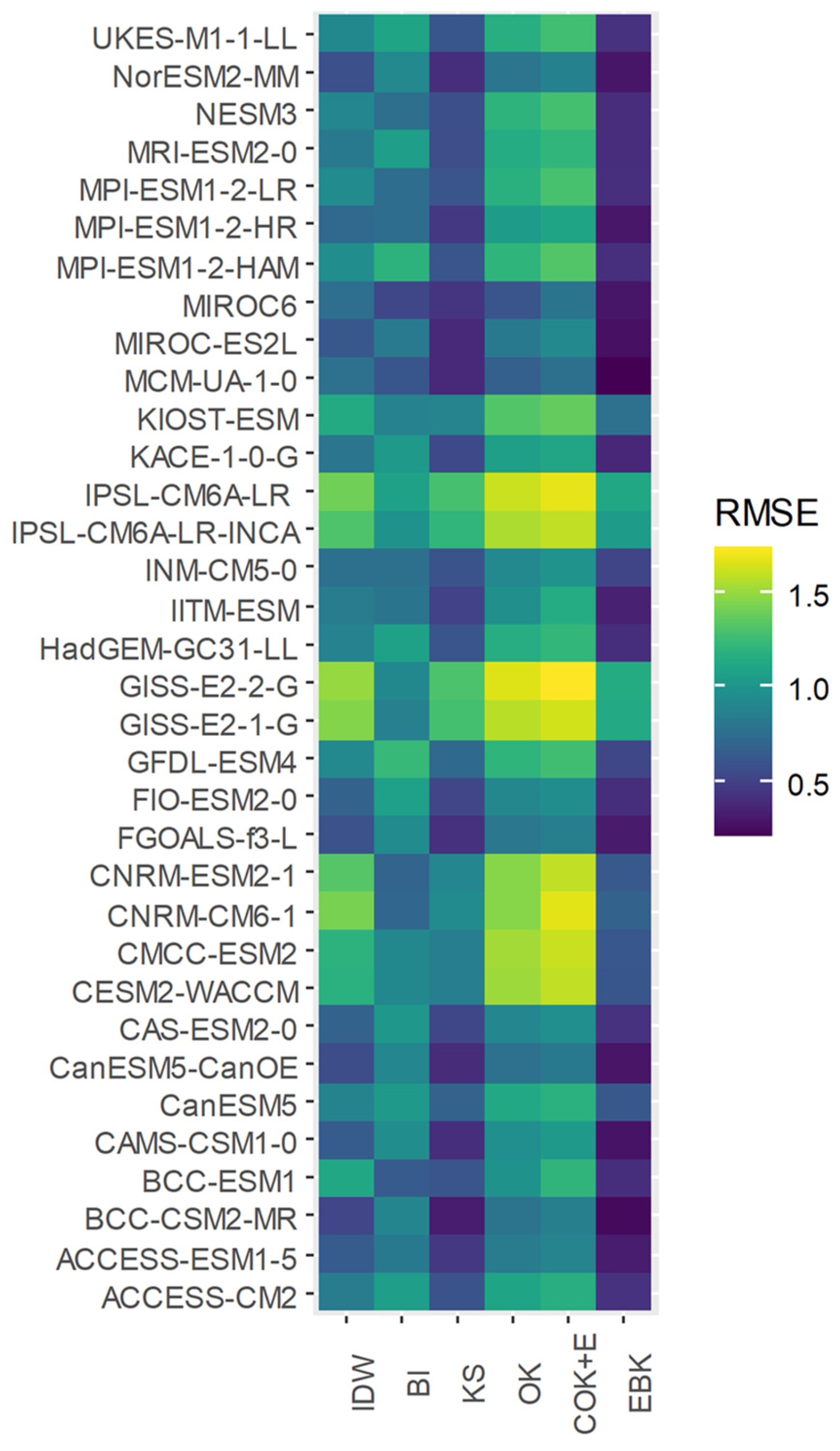
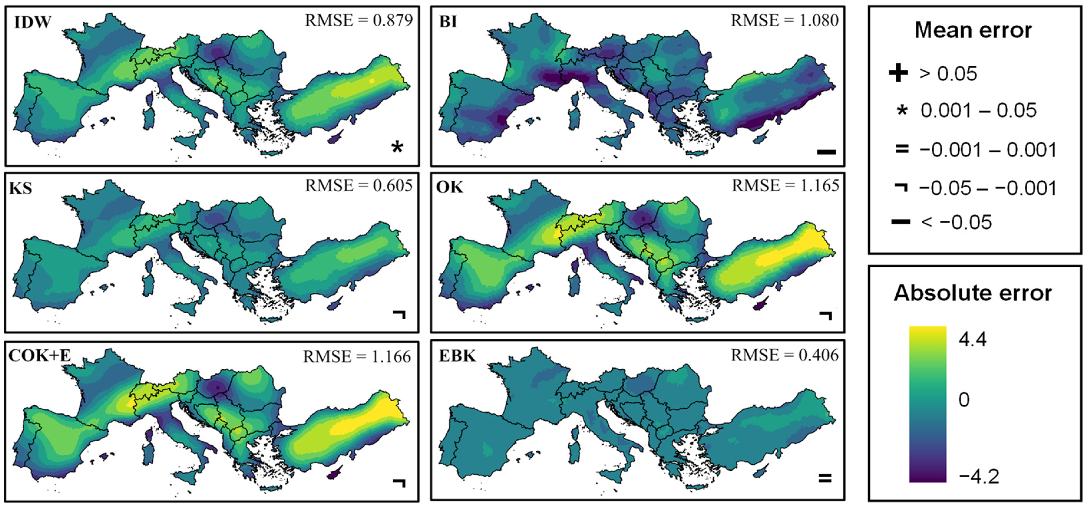
• Empirical Bayesian Kriging (EBK) stands out as the least data-modifying approach for downscaling GCMs and aligning them with ERA5 Land resolution (0.1°). Its Mean Error (ME) is close to 0 °C, while its Root Mean Square Error (RMSE) is less than 0.5 °C. Moreover, its performance is notable across all models and does not exhibit significant errors in specific areas of the study region, even performing well in mountainous regions. Other Kriging methods, particularly Cokriging, yield discouraging results. Bilinear interpolation (BI), the most commonly used GCM downscaling method to date, tends to underestimate temperatures significantly; thus, we do not recommend its use for these purposes.
• MPI-ESM1-2-HR, GFDL-ESM4, CNRM-CM6-1, MRI-ESM2-0, CNRM-ESM2-1, and IPSL-CM6A-LR are the top six GCMs regarding annual temperature simulation in the Euro-Med region across all five metrics used in the assessment. On the other hand, the MCM-UA-1-0 model and the MIROC models demonstrate poor simulation and should not be used in this region of the globe.
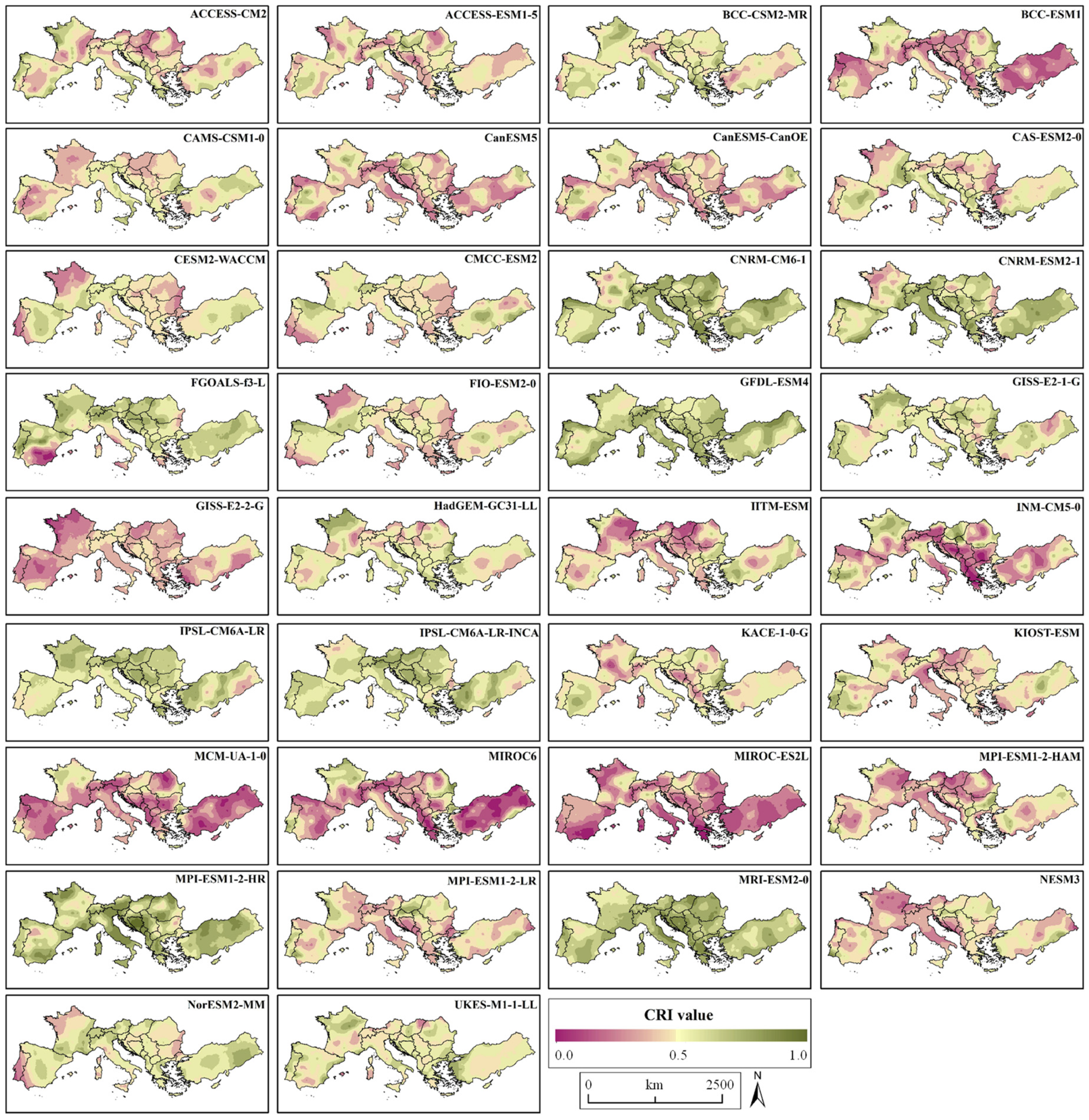
• Significant geospatial differences exist in the performance of GCMs across the Euro-Med region. MPI-ESM1-2-HR performs better in elevated regions such as the Alps, Sierra Nevada, and Carpathian Mountains but fails in the Central Iberian and French areas. GFDL-ESM4 and MRI-ESM2-0 demonstrate more consistent performance across the region. The CNRM models excel in simulating the Cantabrian coast and Greece but fall short in the northwestern half of France. Models from the Hadley Center and FGOALS-f3-L perform well in simulating the Northwestern Iberian and French regions. The MIROC, MCM-UA-1-0, GISS-E2-2-G, and BCC-ESM1 models exhibit mean performance values below 0.25 in any area.
• The optimal number of GCMs for ensemble was determined to be six, maximizing the correlation (0.97) and explained variance (0.93). The Random Forest Ensemble (RFE) method effectively replicates the interannual temperature variability. Additionally, it positively correlates with the ranking value assigned to each GCM (rho = 0.23), although it overestimates the relevance of models with high correlation with the reanalyzed temperature, such as the GFDL-ESM4.
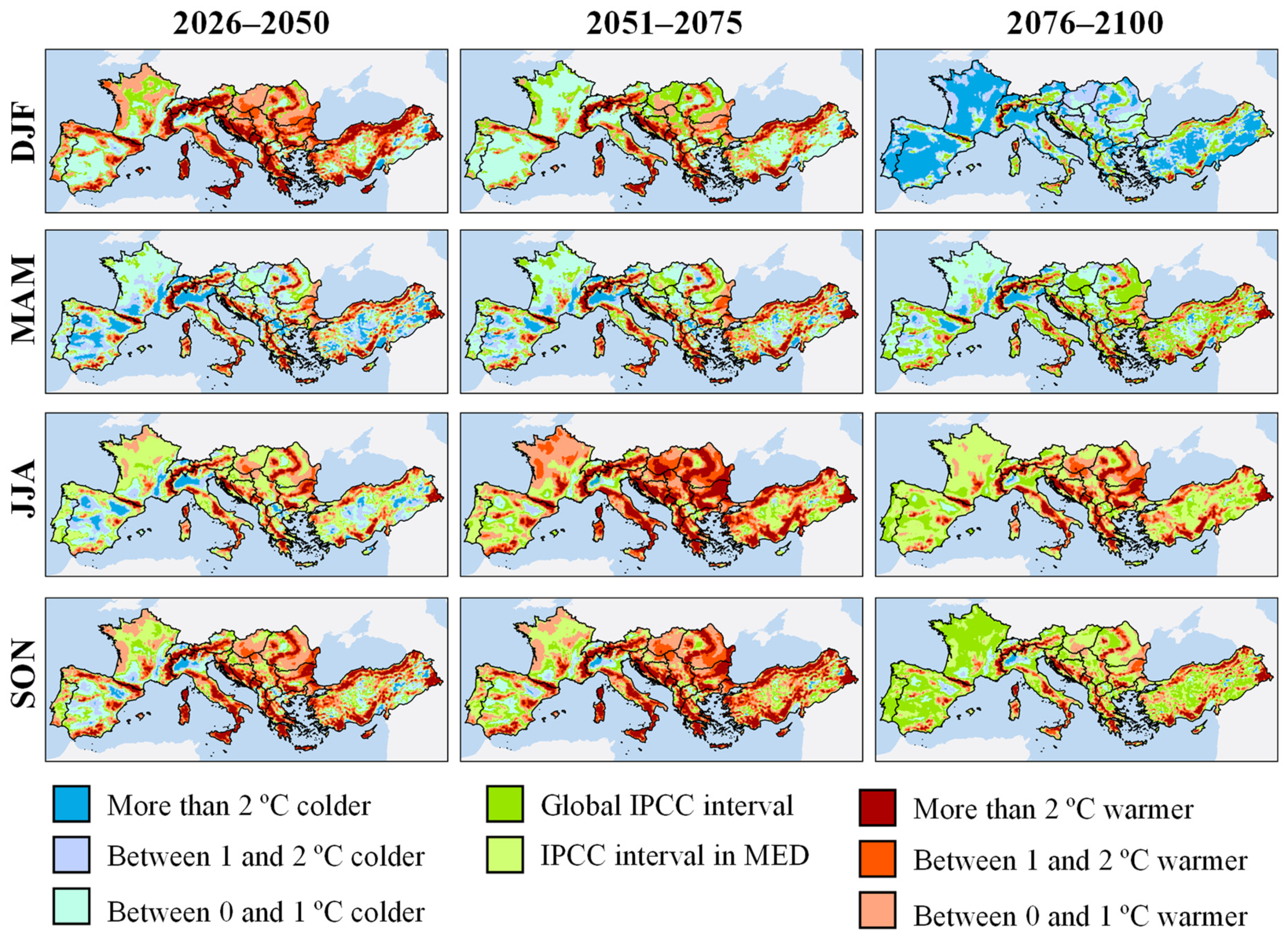
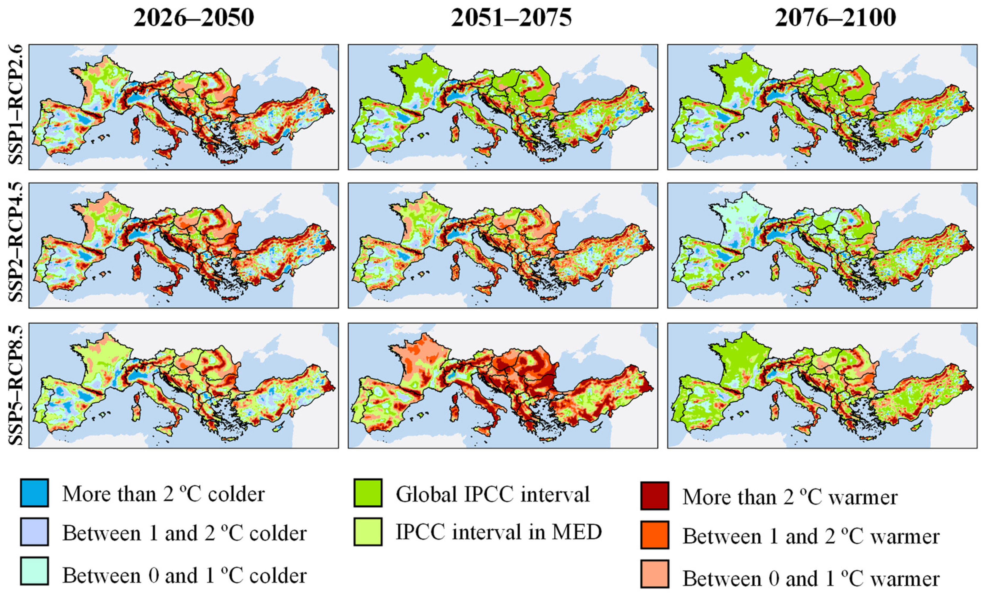
• Significant differences arise between the projections made using the method applied in our research and the IPCC projections at both the global and regional scales. Winter temperatures in the medium-to-long term, particularly in spring, warm up between 1 and more than 2 °C less than what the IPCC expects for any emission scenario. On the other hand, winter temperatures in the short term and summer and autumn temperatures in the short-to-medium term warm up between 1 and more than 2 °C more than expected. The warming is especially found in the higher-elevation regions of the study area and in the Mediterranean islands, where temperatures increase by more than 2 °C compared to the official predictions in all scenarios. In the long term, the projections for summer and autumn in our research show broad agreement with the IPCC confidence interval, exceeding 70% in the pessimistic scenario (SSP5-RCP8.5).

Finally, it is important to highlight that reducing the existing uncertainty in temperature projections at a regional scale is crucial for addressing the adaptive challenges posed by climate change [154], especially in regions as climatically vulnerable as the European Mediterranean region. Adopting appropriate adaptive policies to cope with the consequences of climate change requires an analysis that addresses critical aspects in the modeling chain: downscaling, model selection, and selection of future scenarios [151]. We believe that the method and results of our study can support subsequent research, help establish policy measures that address the challenge of global warming from a holistic perspective, and provide information to territorial planners and environmental conservation organizations to continue their efforts to raise awareness about the importance of mitigation and adaptation to Anthropocene climate change.

References

1. Weart, S. The Discovery of Rapid Climate Change. Phys. Today 2003, 56, 30–36. [Google Scholar] [CrossRef]
2. Jones, P.D.; Wigley, T.M.L.; Folland, C.K.; Parker, D.E.; Angell, J.K.; Lebedeff, S.; Hansen, J.E. Evidence for Global Warming in the Past Decade. Nature 1988, 332, 790. [Google Scholar] [CrossRef]
3. IPCC. Climate Change 2014. Impacts, Adaptation, and Vulnerability. Part B: Regional Aspects; Barros, V.R., Field, C.B., Eds.; Cambridge University Press: New York, NY, USA, 2014. [Google Scholar]
4. IPCC. Climate Change 2021: The Physical Science Basis. Contribution of Working Group I to the Sixth Assessment Report of the Intergovernmental Panel on Climate Change; Masson-Delmotte, V., Zhai, P., Pirani, A., Connors, S.L., Péan, C., Berger, S., Caud, N., Chen, Y., Goldfarb, L., Gomis, M.I., et al., Eds.; Cambridge University Press: New York, NY, USA, 2021. [Google Scholar]
5. Koutsoyiannis, D. Revisiting the Global Hydrological Cycle: Is It Intensifying? Hydrol. Earth Syst. Sci. 2020, 24, 3899–3932. [Google Scholar] [CrossRef]
6. Otto, F.E.L. Attribution of Extreme Events to Climate Change. Annu. Rev. Environ. Resour. 2023, 48, 813–828. [Google Scholar] [CrossRef]
7. Cavicchia, L.; von Storch, H.; Gualdi, S. A Long-Term Climatology of Medicanes. Clim. Dyn. 2014, 43, 1183–1195. [Google Scholar] [CrossRef]
8. Carvalho, L.M.V. Assessing Precipitation Trends in the Americas with Historical Data: A Review. Wiley Interdiscip. Rev. Clim. Change 2020, 11, e627. [Google Scholar] [CrossRef]
9. Meng, Y.; Hao, Z.; Feng, S.; Zhang, X.; Hao, F. Increase in Compound Dry-Warm and Wet-Warm Events under Global Warming in CMIP6 Models. Glob. Planet. Change 2022, 210, 103773. [Google Scholar] [CrossRef]
10. Li, M.; Wu, P.; Sexton, D.M.H.; Ma, Z. Potential Shifts in Climate Zones under a Future Global Warming Scenario Using Soil Moisture Classification. Clim. Dyn. 2021, 56, 2071–2092. [Google Scholar] [CrossRef]
11. Wakatsuki, H.; Ju, H.; Nelson, G.C.; Farrell, A.D.; Deryng, D.; Meza, F.; Hasegawa, T. Research Trends and Gaps in Climate Change Impacts and Adaptation Potentials in Major Crops. Curr. Opin. Environ. Sustain. 2023, 60, 101249. [Google Scholar] [CrossRef]
12. Wang, S.; Zhu, J.; Huang, G.; Baetz, B.; Cheng, G.; Zeng, X.; Wang, X. Assessment of Climate Change Impacts on Energy Capacity Planning in Ontario, Canada Using High-Resolution Regional Climate Model. J. Clean. Prod. 2020, 274, 123026. [Google Scholar] [CrossRef]
13. Loucks, D.P. Meeting Climate Change Challenges: Searching for More Adaptive and Innovative Decisions. Water Resour. Manag. 2023, 37, 2235–2245. [Google Scholar] [CrossRef]
14. Si, X.; Wang, L.; Mengersen, K.; Hu, W. Epidemiological Features of Seasonal Influenza Transmission among 11 Climate Zones in Chinese Mainland. Infect. Dis. Poverty 2024, 13, 4. [Google Scholar] [CrossRef]
15. Cork, S.; Alexandra, C.; Alvarez-Romero, J.G.; Bennett, E.M.; Berbés-Blázquez, M.; Bohensky, E.; Bok, B.; Costanza, R.; Hashimoto, S.; Hill, R.; et al. Exploring Alternative Futures in the Anthropocene. Annu. Rev. Environ. Resour. 2023, 48, 25–54. [Google Scholar] [CrossRef]
16. Paravantis, J.; Santamouris, M.; Cartalis, C.; Efthymiou, C.; Kontoulis, N. Mortality Associated with High Ambient Temperatures, Heatwaves, and the Urban Heat Island in Athens, Greece. Sustainability 2017, 9, 606. [Google Scholar] [CrossRef]
17. O’Neill, B.C.; Oppenheimer, M.; Warren, R.; Hallegatte, S.; Kopp, R.E.; Pörtner, H.O.; Scholes, R.; Birkmann, J.; Foden, W.; Licker, R.; et al. IPCC Reasons for Concern Regarding Climate Change Risks. Nat. Clim. Change 2017, 7, 28–37. [Google Scholar] [CrossRef]
18. Fried, C.; Huybers, P. A Simple Relationship between the Magnitude and Spatial Extent of Global Surface Temperature Anomalies. Geophys. Res. Lett. 2024, 51, e2023GL106537. [Google Scholar] [CrossRef]
19. Sun, C.; Zhu, L.; Liu, Y.; Wei, T.; Guo, Z. CMIP6 Model Simulation of Concurrent Continental Warming Holes in Eurasia and North America since 1990 and Their Relation to the Indo-Pacific SST Warming. Glob. Planet. Change 2022, 213, 103824. [Google Scholar] [CrossRef]
20. Dai, T.; Dong, W.; Sun, S.; Wang, G. Exploring the Asymmetry and Rate of SAT Warming over the Global Land Area under the 1.5 °C and 2 °C Climate Change Targets. Meteorol. Atmos. Phys. 2023, 135, 19. [Google Scholar] [CrossRef]
21. Rivas-Martínez, S.; Rivas-Sáenz, S.; Penas, Á. Worldwide Bioclimatic Classification System. Glob. Geobot. 2011, 1, 1–634. [Google Scholar] [CrossRef]
22. Tramblay, Y.; Koutroulis, A.; Samaniego, L.; Vicente-Serrano, S.M.; Volaire, F.; Boone, A.; Le Page, M.; Llasat, M.C.; Albergel, C.; Burak, S.; et al. Challenges for Drought Assessment in the Mediterranean Region under Future Climate Scenarios. Earth Sci. Rev. 2020, 210, 103348. [Google Scholar] [CrossRef]
23. Polade, S.D.; Gershunov, A.; Cayan, D.R.; Dettinger, M.D.; Pierce, D.W. Precipitation in a Warming World: Assessing Projected Hydro-Climate Changes in California and Other Mediterranean Climate Regions. Sci. Rep. 2017, 7, 10783. [Google Scholar] [CrossRef] [PubMed]
24. Giorgi, F.; Raffaele, F. On the Dependency of GCM-Based Regional Surface Climate Change Projections on Model Biases, Resolution and Climate Sensitivity. Clim. Dyn. 2022, 58, 2843–2862. [Google Scholar] [CrossRef]
25. Diffenbaugh, N.S.; Swain, D.L.; Touma, D.; Lubchenco, J. Anthropogenic Warming Has Increased Drought Risk in California. Proc. Natl. Acad. Sci. USA 2015, 112, 3931–3936. [Google Scholar] [CrossRef] [PubMed]
26. González-Pérez, A.; Álvarez-Esteban, R.; Penas, Á.; Del Río, S. Analysis of Recent Mean Temperature Trends and Relationships with Teleconnection Patterns in California (U.S.). Appl. Sci. 2022, 12, 5831. [Google Scholar] [CrossRef]
27. Adeola, A.M.; Kruger, A.; Makgoale, T.E.; Botai, J.O. Observed Trends and Projections of Temperature and Precipitation in the Olifants River Catchment in South Africa. PLoS ONE 2022, 17, e0271974. [Google Scholar] [CrossRef]
28. Ndlovu, M.; Clulow, A.D.; Savage, M.J.; Nhamo, L.; Magidi, J.; Mabhaudhi, T. An Assessment of the Impacts of Climate Variability and Change in Kwazulu-Natal Province, South Africa. Atmosphere 2021, 12, 427. [Google Scholar] [CrossRef]
29. Trancoso, R.; Syktus, J.; Toombs, N.; Ahrens, D.; Wong, K.K.H.; Pozza, R.D. Heatwaves Intensification in Australia: A Consistent Trajectory across Past, Present and Future. Sci. Total Environ. 2020, 742, 140521. [Google Scholar] [CrossRef] [PubMed]
30. MedECC. Climate and Environmental Change in the Mediterranean Basin—Current Situation and Risks for the Future. First Mediterranean Assessment Report; Cramer, W., Guiot, J., Marini, K., Eds.; Mediterranean Experts on Climate and Environmental Change (MedECC): Marseille, France, 2020. [Google Scholar]
31. Fan, X.; Duan, Q.; Shen, C.; Wu, Y.; Xing, C. Global Surface Air Temperatures in CMIP6: Historical Performance and Future Changes. Environ. Res. Lett. 2020, 15, 104056. [Google Scholar] [CrossRef]
32. Almazroui, M.; Ashfaq, M.; Islam, M.N.; Rashid, I.U.; Kamil, S.; Abid, M.A.; O’Brien, E.; Ismail, M.; Reboita, M.S.; Sörensson, A.A.; et al. Assessment of CMIP6 Performance and Projected Temperature and Precipitation Changes Over South America. ESEV 2021, 5, 155–183. [Google Scholar] [CrossRef]
33. Zhao, Y.; Qian, C.; Zhang, W.; He, D.; Qi, Y. Extreme Temperature Indices in Eurasia in a CMIP6 Multi-Model Ensemble: Evaluation and Projection. Int. J. Climatol. 2021, 41, 5368–5385. [Google Scholar] [CrossRef]
34. Shi, J.; Tian, Z.; Lang, X.; Jiang, D. Projected Changes in the Interannual Variability of Surface Air Temperature Using CMIP6 Simulations. Clim. Dyn. 2023, 62, 431–446. [Google Scholar] [CrossRef]
35. Yang, X.; Zhou, B.; Xu, Y.; Han, Z. CMIP6 Evaluation and Projection of Temperature and Precipitation over China. Adv. Atmos. Sci. 2021, 38, 817–830. [Google Scholar] [CrossRef]
36. Overpeck, J.T.; Meehl, G.A.; Bony, S.; Easterling, D.R. Climate Data Challenges in the 21st Century. Science 2011, 331, 700–702. [Google Scholar] [CrossRef]
37. Hausfather, Z.; Drake, H.F.; Abbott, T.; Schmidt, G.A. Evaluating the Performance of Past Climate Model Projections. Geophys. Res. Lett. 2020, 47, e2019GL085378. [Google Scholar] [CrossRef]
38. Balaji, V.; Couvreux, F.; Deshayes, J.; Gautrais, J.; Hourdin, F.; Rio, C. Are General Circulation Models Obsolete? Proc. Natl. Acad. Sci. USA 2022, 119, e2202075119. [Google Scholar] [CrossRef] [PubMed]
39. Eyring, V.; Bony, S.; Meehl, G.A.; Senior, C.A.; Stevens, B.; Stouffer, R.J.; Taylor, K.E. Overview of the Coupled Model Intercomparison Project Phase 6 (CMIP6) Experimental Design and Organization. Geosci. Model. Dev. 2016, 9, 1937–1958. [Google Scholar] [CrossRef]
40. Brands, S. A Circulation-Based Performance Atlas of the CMIP5 and 6 Models for Regional Climate Studies in the Northern Hemisphere Mid-to-High Latitudes. Geosci. Model. Dev. 2022, 15, 1375–1411. [Google Scholar] [CrossRef]
41. Fernandez-Granja, J.A.; Casanueva, A.; Bedia, J.; Fernandez, J. Improved Atmospheric Circulation over Europe by the New Generation of CMIP6 Earth System Models. Clim. Dyn. 2021, 56, 3527–3540. [Google Scholar] [CrossRef]
42. Xia, Y.; Hu, Y.; Liu, J. Comparison of Trends in the Hadley Circulation between CMIP6 and CMIP5. Sci. Bull. 2020, 65, 1667–1674. [Google Scholar] [CrossRef] [PubMed]
43. Fan, X.; Miao, C.; Duan, Q.; Shen, C.; Wu, Y. The Performance of CMIP6 versus CMIP5 in Simulating Temperature Extremes Over the Global Land Surface. J. Geophys. Res.-Atmos. 2020, 125, e2020JD033031. [Google Scholar] [CrossRef]
44. Guo, H.; Zhan, C.; Ning, L.; Li, Z.; Hu, S. Evaluation and Comparison of CMIP6 and CMIP5 Model Performance in Simulating the Runoff. Theor. Appl. Climatol. 2022, 149, 1451–1470. [Google Scholar] [CrossRef]
45. Li, J.; Huo, R.; Chen, H.; Zhao, Y.; Zhao, T. Comparative Assessment and Future Prediction Using CMIP6 and CMIP5 for Annual Precipitation and Extreme Precipitation Simulation. Front. Earth Sci. 2021, 9, 687976. [Google Scholar] [CrossRef]
46. Cos, J.; Doblas-Reyes, F.; Jury, M.; Marcos, R.; Bretonnière, P.A.; Samsó, M. The Mediterranean Climate Change Hotspot in the CMIP5 and CMIP6 Projections. Earth Syst. Dyn. 2022, 13, 321–340. [Google Scholar] [CrossRef]
47. Zhou, C.; Penner, J.E. Why Do General Circulation Models Overestimate the Aerosol Cloud Lifetime Effect? A Case Study Comparing CAM5 and a CRM. Atmos. Chem. Phys. 2017, 17, 21–29. [Google Scholar] [CrossRef]
48. Boberg, F.; Christensen, J.H. Overestimation of Mediterranean Summer Temperature Projections Due to Model Deficiencies. Nat. Clim. Change 2012, 2, 433–436. [Google Scholar] [CrossRef]
49. Das, R.S.; Rao, S.A.; Pillai, P.A.; Srivastava, A.; Pradhan, M.; Ramu, D.A. Why Coupled General Circulation Models Overestimate the ENSO and Indian Summer Monsoon Rainfall (ISMR) Relationship? Clim. Dyn. 2022, 59, 2995–3011. [Google Scholar] [CrossRef]
50. Loehle, C. The Epistemological Status of General Circulation Models. Clim. Dyn. 2018, 50, 1719–1731. [Google Scholar] [CrossRef]
51. Maraun, D.; Truhetz, H.; Schaffer, A. Regional Climate Model Biases, Their Dependence on Synoptic Circulation Biases and the Potential for Bias Adjustment: A Process-Oriented Evaluation of the Austrian Regional Climate Projections. J. Geophys. Res.-Atmos. 2021, 126, e2020JD032824. [Google Scholar] [CrossRef]
52. Ali, Z.; Hamed, M.M.; Muhammad, M.K.I.; Iqbal, Z.; Shahid, S. Performance Evaluation of CMIP6 GCMs for the Projections of Precipitation Extremes in Pakistan. Clim. Dyn. 2023, 61, 4717–4732. [Google Scholar] [CrossRef]
53. Feyissa, T.A.; Demissie, T.A.; Saathoff, F.; Gebissa, A. Evaluation of General Circulation Models CMIP6 Performance and Future Climate Change over the Omo River Basin, Ethiopia. Sustainability 2023, 15, 6507. [Google Scholar] [CrossRef]
54. Nguyen-Duy, T.; Ngo-Duc, T.; Desmet, Q. Performance Evaluation and Ranking of CMIP6 Global Climate Models over Vietnam. J. Water Clim. Change 2023, 14, 1831–1846. [Google Scholar] [CrossRef]
55. Peng, S.; Wang, C.; Li, Z.; Mihara, K.; Kuramochi, K.; Toma, Y.; Hatano, R. Climate Change Multi-Model Projections in CMIP6 Scenarios in Central Hokkaido, Japan. Sci. Rep. 2023, 13, 230. [Google Scholar] [CrossRef] [PubMed]
56. Sa’adi, Z.; Alias, N.E.; Yusop, Z.; Iqbal, Z.; Houmsi, M.R.; Houmsi, L.N.; Ramli, M.W.A.; Muhammad, M.K.I. Application of Relative Importance Metrics for CMIP6 Models Selection in Projecting Basin-Scale Rainfall over Johor River Basin, Malaysia. Sci. Total Environ. 2024, 912, 169187. [Google Scholar] [CrossRef] [PubMed]
57. Raju, K.S.; Kumar, D.N. Review of Approaches for Selection and Ensembling of GCMs. J. Water Clim. Change 2020, 11, 577–599. [Google Scholar] [CrossRef]
58. Abadie, L.M.; Moral, M.P. A Method for Selecting a Climate Model: An Application for Maximum Daily Temperature in Southern Spain. Theor. Appl. Climatol. 2023, 152, 773–786. [Google Scholar] [CrossRef]
59. Peres, D.J.; Senatore, A.; Nanni, P.; Cancelliere, A.; Mendicino, G.; Bonaccorso, B. Evaluation of EURO-CORDEX (Coordinated Regional Climate Downscaling Experiment for the Euro-Mediterranean Area) Historical Simulations by High-Quality Observational Datasets in Southern Italy: Insights on Drought Assessment. Nat. Hazard Earth Syst. 2020, 20, 3057–3082. [Google Scholar] [CrossRef]
60. Bağçaci, S.Ç.; Yucel, I.; Duzenli, E.; Yilmaz, M.T. Intercomparison of the Expected Change in the Temperature and the Precipitation Retrieved from CMIP6 and CMIP5 Climate Projections: A Mediterranean Hot Spot Case, Turkey. Atmos. Res. 2021, 256, 105576. [Google Scholar] [CrossRef]
61. Seker, M.; Gumus, V. Projection of Temperature and Precipitation in the Mediterranean Region through Multi-Model Ensemble from CMIP6. Atmos. Res. 2022, 280, 106440. [Google Scholar] [CrossRef]
62. Jury, M.W.; Prein, A.F.; Truhetz, H.; Gobiet, A. Evaluation of CMIP5 Models in the Context of Dynamical Downscaling over Europe. J. Clim. 2015, 28, 5575–5582. [Google Scholar] [CrossRef]
63. Palmer, T.E.; Booth, B.B.B.; McSweeney, C.F. How Does the CMIP6 Ensemble Change the Picture for European Climate Projections? Environ. Res. Lett. 2021, 16, 094042. [Google Scholar] [CrossRef]
64. Tuel, A.; Kang, S.; Eltahir, E.A.B. Understanding Climate Change over the Southwestern Mediterranean Using High-Resolution Simulations. Clim. Dyn. 2021, 56, 985–1001. [Google Scholar] [CrossRef]
65. Drobinski, P.; Da Silva, N.; Bastin, S.; Mailler, S.; Muller, C.; Ahrens, B.; Christensen, O.B.; Lionello, P. How Warmer and Drier Will the Mediterranean Region Be at the End of the Twenty-First Century? Reg. Environ. Change 2020, 20, 78. [Google Scholar] [CrossRef]
66. Todaro, V.; D’Oria, M.; Secci, D.; Zanini, A.; Tanda, M.G. Climate Change over the Mediterranean Region: Local Temperature and Precipitation Variations at Five Pilot Sites. Water 2022, 14, 2499. [Google Scholar] [CrossRef]
67. Zittis, G.; Hadjinicolaou, P.; Klangidou, M.; Proestos, Y.; Lelieveld, J.A. Multi-Model, Multi-Scenario, and Multi-Domain Analysis of Regional Climate Projections for the Mediterranean. Reg. Environ. Change 2019, 19, 2621–2635. [Google Scholar] [CrossRef]
68. Zhang, L.; Jiapaer, G.; Yu, T.; Umuhoza, J.; Tu, H.; Chen, B.; Liang, H.; Lin, K.; Ju, T.; De Maeyer, P.; et al. Evaluating and Correcting Temperature and Precipitation Grid Products in the Arid Region of Altay, China. Remote Sens. 2024, 16, 283. [Google Scholar] [CrossRef]
69. Sun, P.; Zou, Y.; Yao, R.; Ma, Z.; Bian, Y.; Ge, C.; Lv, Y. Compound and Successive Events of Extreme Precipitation and Extreme Runoff under Heatwaves Based on CMIP6 Models. Sci. Total Environ. 2023, 878, 162980. [Google Scholar] [CrossRef] [PubMed]
70. Christian, J.R.; Denman, K.L.; Hayashida, H.; Holdsworth, A.M.; Lee, W.G.; Riche, O.G.J.; Shao, A.E.; Steiner, N.; Swart, N.C. Ocean Biogeochemistry in the Canadian Earth System Model Version 5.0.3: CanESM5 and CanESM5-CanOE. Geosci. Model. Dev. 2022, 15, 4393–4424. [Google Scholar] [CrossRef]
71. Salzmann, M.; Ferrachat, S.; Tully, C.; Münch, S.; Watson-Parris, D.; Neubauer, D.; Siegenthaler-Le Drian, C.; Rast, S.; Heinold, B.; Crueger, T.; et al. The Global Atmosphere-Aerosol Model ICON-A-HAM2.3–Initial Model Evaluation and Effects of Radiation Balance Tuning on Aerosol Optical Thickness. J. Adv. Model. Earth Syst. 2022, 14, e2021MS002699. [Google Scholar] [CrossRef] [PubMed]
72. Schmid, S.M.; Fügenschuh, B.; Kissling, E.; Schuster, R. Tectonic Map and Overall Architecture of the Alpine Orogen. Eclogae Geol. Helv. 2004, 97, 93–117. [Google Scholar] [CrossRef]
73. Holdridge, L.R. Life Zone Ecology; Tropical Science Center: San Pedro de Montes de Oca, Costa Rica, 1967. [Google Scholar]
74. WMO. Updated 30-Year Reference Period Reflects Changing Climate. Available online: https://public.wmo.int/en/media/news/updated-30-year-reference-period-reflects-changing-climate (accessed on 5 May 2023).
75. Muñoz-Sabater, J.; Dutra, E.; Agustí-Panareda, A.; Albergel, C.; Arduini, G.; Balsamo, G.; Boussetta, S.; Choulga, M.; Harrigan, S.; Hersbach, H.; et al. ERA5-Land: A State-of-the-Art Global Reanalysis Dataset for Land Applications. Earth Syst. Sci. Data 2021, 13, 4349–4383. [Google Scholar] [CrossRef]
76. Zou, J.; Lu, N.; Jiang, H.; Qin, J.; Yao, L.; Xin, Y.; Su, F. Performance of Air Temperature from ERA5-Land Reanalysis in Coastal Urban Agglomeration of Southeast China. Sci. Total Environ. 2022, 828, 154459. [Google Scholar] [CrossRef]
77. De Araújo, C.S.P.; Silva, I.A.C.E.; Ippolito, M.; de Almeida, C.D.G.C. Evaluation of Air Temperature Estimated by ERA5-Land Reanalysis Using Surface Data in Pernambuco, Brazil. Environ. Monit. Assess. 2022, 194, 381. [Google Scholar] [CrossRef]
78. Zhao, P.; He, Z. A First Evaluation of ERA5-Land Reanalysis Temperature Product over the Chinese Qilian Mountains. Front. Earth Sci. 2022, 10, 907730. [Google Scholar] [CrossRef]
79. Barbosa, S.; Scotto, M.G. Extreme Heat Events in the Iberia Peninsula from Extreme Value Mixture Modeling of ERA5-Land Air Temperature. Weather Clim. Extrem. 2022, 36, 100448. [Google Scholar] [CrossRef]
80. Pelosi, A.; Terribile, F.; D’Urso, G.; Chirico, G.B. Comparison of ERA5-Land and UERRA MESCAN-SURFEX Reanalysis Data with Spatially Interpolated Weather Observations for the Regional Assessment of Reference Evapotranspiration. Water 2020, 12, 1669. [Google Scholar] [CrossRef]
81. Liu, J.; Fiifi, D.; Hagan, T.; Liu, Y.; Liu, J.; Hagan, D.F.T.; Liu, Y. Global Land Surface Temperature Change (2003–2017) and Its Relationship with Climate Drivers: AIRS, MODIS, and ERA5-Land Based Analysis. Remote Sens. 2021, 13, 44. [Google Scholar] [CrossRef]
82. Yilmaz, M. Consistency of Spatiotemporal Variability of MODIS and ERA5-Land Surface Warming Trends over Complex Topography. Environ. Sci. Pollut. R 2023, 30, 94414–94435. [Google Scholar] [CrossRef]
83. Tan, M.L.; Armanuos, A.M.; Ahmadianfar, I.; Demir, V.; Heddam, S.; Al-Areeq, A.M.; Abba, S.I.; Halder, B.; Cagan Kilinc, H.; Yaseen, Z.M. Evaluation of NASA POWER and ERA5-Land for Estimating Tropical Precipitation and Temperature Extremes. J. Hydrol. 2023, 624, 129940. [Google Scholar] [CrossRef]
84. Scafetta, N. Testing the CMIP6 GCM Simulations versus Surface Temperature Records from 1980–1990 to 2011–2021: High ECS Is Not Supported. Climate 2021, 9, 161. [Google Scholar] [CrossRef]
85. Collazo, S.; Barrucand, M.; Rusticucci, M. Evaluation of CMIP6 Models in the Representation of Observed Extreme Temperature Indices Trends in South America. Clim. Change 2022, 172, 21. [Google Scholar] [CrossRef]
86. Ali, Z.; Hamed, M.M.; Muhammad, M.K.I.; Shahid, S. A Novel Approach for Evaluation of CMIP6 GCMs in Simulating Temperature and Precipitation Extremes of Pakistan. Int. J. Climatol. 2024, 44, 592–612. [Google Scholar] [CrossRef]
87. Blanke, J.H.; Lindeskog, M.; Lindström, J.; Lehsten, V. Effect of Climate Data on Simulated Carbon and Nitrogen Balances for Europe. J. Geophys. Res. Biogeosci. 2016, 121, 1352–1371. [Google Scholar] [CrossRef]
88. Graux, A.I.; Bellocchi, G.; Lardy, R.; Soussana, J.F. Ensemble Modelling of Climate Change Risks and Opportunities for Managed Grasslands in France. Agric. For. Meteorol. 2013, 170, 114–131. [Google Scholar] [CrossRef]
89. Čejka, T.; Trnka, M.; Krusic, P.J.; Stobbe, U.; Oliach, D.; Václavík, T.; Tegel, W.; Büntgen, U. Predicted Climate Change Will Increase the Truffle Cultivation Potential in Central Europe. Sci. Rep. 2020, 10, 21281. [Google Scholar] [CrossRef]
90. Chilès, J.-P.; Desassis, N. Fifty Years of Kriging. In Handbook of Mathematical Geosciences; Daya Sagar, B.S., Cheng, Q., Agterberg, F., Eds.; Springer: Cham, Switzerland, 2018; pp. 589–612. [Google Scholar]
91. Mühlenstädt, T.; Kuhnt, S. Kernel Interpolation. Comput. Stat. Data Anal. 2011, 55, 2962–2974. [Google Scholar] [CrossRef]
92. Antal, A.; Guerreiro, P.M.P.; Cheval, S. Comparison of Spatial Interpolation Methods for Estimating the Precipitation Distribution in Portugal. Theor. Appl. Climatol. 2021, 145, 1193–1206. [Google Scholar] [CrossRef]
93. Katipoğlu, O.M. Spatial Analysis of Seasonal Precipitation Using Various Interpolation Methods in the Euphrates Basin, Turkey. Acta Geophys. 2022, 70, 859–878. [Google Scholar] [CrossRef]
94. ESRI ArcGIS 2019. Available online: https://www.esri.com/en-us/arcgis/products/arcgis-desktop (accessed on 28 January 2023).
95. Di Virgilio, G.; Ji, F.; Tam, E.; Nishant, N.; Evans, J.P.; Thomas, C.; Riley, M.L.; Beyer, K.; Grose, M.R.; Narsey, S.; et al. Selecting CMIP6 GCMs for CORDEX Dynamical Downscaling: Model Performance, Independence, and Climate Change Signals. Earth’s Future 2022, 10, e2021EF002625. [Google Scholar] [CrossRef]
96. Lei, X.; Xu, C.; Liu, F.; Song, L.; Cao, L.; Suo, N. Evaluation of CMIP6 Models and Multi-Model Ensemble for Extreme Precipitation over Arid Central Asia. Remote Sens. 2023, 15, 2376. [Google Scholar] [CrossRef]
97. Jiang, Z.; Li, W.; Xu, J.; Li, L. Extreme Precipitation Indices over China in CMIP5 Models. Part I: Model Evaluation. J. Clim. 2015, 28, 8603–8619. [Google Scholar] [CrossRef]
98. Wang, B.; Zheng, L.; Liu, D.L.; Ji, F.; Clark, A.; Yu, Q. Using Multi-Model Ensembles of CMIP5 Global Climate Models to Reproduce Observed Monthly Rainfall and Temperature with Machine Learning Methods in Australia. Int. J. Climatol. 2018, 38, 4891–4902. [Google Scholar] [CrossRef]
99. Hernanz, A.; García-Valero, J.A.; Domínguez, M.; Rodríguez-Camino, E. Evaluation of Statistical Downscaling Methods for Climate Change Projections over Spain: Present Conditions with Imperfect Predictors (Global Climate Model Experiment). Int. J. Climatol. 2022, 42, 6793–6806. [Google Scholar] [CrossRef]
100. Ahmed, K.; Sachindra, D.A.; Shahid, S.; Iqbal, Z.; Nawaz, N.; Khan, N. Multi-Model Ensemble Predictions of Precipitation and Temperature Using Machine Learning Algorithms. Atmos. Res. 2020, 236, 104806. [Google Scholar] [CrossRef]
101. Breiman, L. Random Forests. Mach. Learn. 2001, 45, 5–32. [Google Scholar] [CrossRef]
102. O’Neill, B.C.; Tebaldi, C.; Van Vuuren, D.P.; Eyring, V.; Friedlingstein, P.; Hurtt, G.; Knutti, R.; Kriegler, E.; Lamarque, J.F.; Lowe, J.; et al. The Scenario Model Intercomparison Project (ScenarioMIP) for CMIP6. Geosci. Model. Dev. 2016, 9, 3461–3482. [Google Scholar] [CrossRef]
103. Gutiérrez, J.M.; Jones, R.G.; Narisma, G.T.; Alves, L.M.; Amjad, M.; Gorodetskaya, I.V.; Grose, M.; Klutse, N.A.B.; Krakovska, S.; Li, J.; et al. 2021: Atlas. In Climate Change 2021: The Physical Science Basis. Contribution of Working Group I to the Sixth Assessment Report of the Intergovernmental Panel on Climate Change; Masson-Delmotte, V.P., Zhai, A., Pirani, S.L., Connors, C., Péan, S., Berger, N., Caud, Y., Chen, L., Goldfarb, M.I., Gomis, M., et al., Eds.; Cambridge University Press: New York, NY, USA, 2021; pp. 1927–1929. [Google Scholar]
104. Liu, A.; Qu, C.; Zhang, J.; Sun, W.; Shi, C.; Lima, A.; De Vivo, B.; Huang, H.; Palmisano, M.; Guarino, A.; et al. Screening and Optimization of Interpolation Methods for Mapping Soil-Borne Polychlorinated Biphenyls. Sci. Total Environ. 2024, 913, 169498. [Google Scholar] [CrossRef] [PubMed]
105. Krivoruchko, K.; Gribov, A. Distance Metrics for Data Interpolation over Large Areas on Earth’s Surface. Spat. Stat. 2020, 35, 100396. [Google Scholar] [CrossRef]
106. Biernacik, P.; Kazimierski, W.; Włodarczyk-Sielicka, M. Comparative Analysis of Selected Geostatistical Methods for Bottom Surface Modeling. Sensors 2023, 23, 3941. [Google Scholar] [CrossRef] [PubMed]
107. Gribov, A.; Krivoruchko, K. Empirical Bayesian Kriging Implementation and Usage. Sci. Total Environ. 2020, 722, 137290. [Google Scholar] [CrossRef]
108. Liu, Z.N.; Yu, X.Y.; Jia, L.F.; Wang, Y.S.; Song, Y.C.; Meng, H.D. The Influence of Distance Weight on the Inverse Distance Weighted Method for Ore-Grade Estimation. Sci. Rep. 2021, 11, 2689. [Google Scholar] [CrossRef]
109. Pellicone, G.; Caloiero, T.; Guagliardi, I. The De Martonne Aridity Index in Calabria (Southern Italy). J. Maps 2019, 15, 788–796. [Google Scholar] [CrossRef]
110. Iqbal, Z.; Shahid, S.; Ahmed, K.; Ismail, T.; Khan, N.; Virk, Z.T.; Johar, W. Evaluation of Global Climate Models for Precipitation Projection in Sub-Himalaya Region of Pakistan. Atmos. Res. 2020, 245, 105061. [Google Scholar] [CrossRef]
111. Ahmed, K.; Sachindra, D.A.; Shahid, S.; Demirel, M.C.; Chung, E.S. Selection of Multi-Model Ensemble of General Circulation Models for the Simulation of Precipitation and Maximum and Minimum Temperature Based on Spatial Assessment Metrics. Hydrol. Earth Syst. Sci. 2019, 23, 4803–4824. [Google Scholar] [CrossRef]
112. Dubrovsky, M.; Trnka, M.; Holman, I.P.; Svobodova, E.; Harrison, P.A. Developing a Reduced-Form Ensemble of Climate Change Scenarios for Europe and Its Application to Selected Impact Indicators. Clim. Change 2015, 128, 169–186. [Google Scholar] [CrossRef]
113. Senent-Aparicio, J.; Pérez-Sánchez, J.; Carrillo-García, J.; Soto, J.; Abbaspour, K.; Srinivasan, R.; Ashraf Vaghefi, S.; Faramarzi, M.; Chen, L. Using SWAT and Fuzzy TOPSIS to Assess the Impact of Climate Change in the Headwaters of the Segura River Basin (SE Spain). Water 2017, 9, 149. [Google Scholar] [CrossRef]
114. Pastor, M.A.; Casado, M.J. Use of Circulation Types Classifications to Evaluate AR4 Climate Models over the Euro-Atlantic Region. Clim. Dyn. 2012, 39, 2059–2077. [Google Scholar] [CrossRef]
115. Topál, D.; Hatvani, I.G.; Kern, Z. Refining Projected Multidecadal Hydroclimate Uncertainty in East-Central Europe Using CMIP5 and Single-Model Large Ensemble Simulations. Theor. Appl. Climatol. 2020, 142, 1147–1167. [Google Scholar] [CrossRef]
116. Adeyeri, O.E.; Zhou, W.; Wang, X.; Zhang, R.; Laux, P.; Ishola, K.A.; Usman, M. The Trend and Spatial Spread of Multisectoral Climate Extremes in CMIP6 Models. Sci. Rep. 2022, 12, 21000. [Google Scholar] [CrossRef] [PubMed]
117. Stryhal, J.; Huth, R. Classifications of Winter Atmospheric Circulation Patterns: Validation of CMIP5 GCMs over Europe and the North Atlantic. Clim. Dyn. 2019, 52, 3575–3598. [Google Scholar] [CrossRef]
118. McSweeney, C.F.; Jones, R.G.; Lee, R.W.; Rowell, D.P. Selecting CMIP5 GCMs for Downscaling over Multiple Regions. Clim. Dyn. 2015, 44, 3237–3260. [Google Scholar] [CrossRef]
119. McMahon, T.A.; Peel, M.C.; Karoly, D.J. Assessment of Precipitation and Temperature Data from CMIP3 Global Climate Models for Hydrologic Simulation. Hydrol. Earth Syst. Sci. 2015, 19, 361–377. [Google Scholar] [CrossRef]
120. Hauglustaine, D.A.; Balkanski, Y.; Schulz, M. A Global Model Simulation of Present and Future Nitrate Aerosols and Their Direct Radiative Forcing of Climate. Atmos. Chem. Phys. 2014, 14, 11031–11063. [Google Scholar] [CrossRef]
121. Crawford, J.; Venkataraman, K.; Booth, J. Developing Climate Model Ensembles: A Comparative Case Study. J. Hydrol. 2019, 568, 160–173. [Google Scholar] [CrossRef]
122. Dey, A.; Sahoo, D.P.; Kumar, R.; Remesan, R. A Multimodel Ensemble Machine Learning Approach for CMIP6 Climate Model Projections in an Indian River Basin. Int. J. Climatol. 2022, 42, 9215–9236. [Google Scholar] [CrossRef]
123. Hussain, M.; Yusof, K.W.; Mustafa, M.R.U.; Mahmood, R.; Jia, S. Evaluation of CMIP5 Models for Projection of Future Precipitation Change in Bornean Tropical Rainforests. Theor. Appl. Climatol. 2018, 134, 423–440. [Google Scholar] [CrossRef]
124. Pielke, R., Jr.; Ritchie, J. How Climate Scenarios Lost Touch With Reality. Issues Sci. Technol. 2021, 37, 74–83. [Google Scholar]
125. Carvalho, D.; Rafael, S.; Monteiro, A.; Rodrigues, V.; Lopes, M.; Rocha, A. How Well Have CMIP3, CMIP5 and CMIP6 Future Climate Projections Portrayed the Recently Observed Warming. Sci. Rep. 2022, 12, 11983. [Google Scholar] [CrossRef] [PubMed]
126. Burgess, M.G.; Ritchie, J.; Shapland, J.; Pielke, R. IPCC Baseline Scenarios Have Over-Projected CO2 Emissions and Economic Growth. Environ. Res. Lett. 2020, 16, 014016. [Google Scholar] [CrossRef]
127. Siegert, M.; Alley, R.B.; Rignot, E.; Englander, J.; Corell, R. Twenty-First Century Sea-Level Rise Could Exceed IPCC Projections for Strong-Warming Futures. One Earth 2020, 3, 691–703. [Google Scholar] [CrossRef]
128. Freychet, N.; Hegerl, G.; Mitchell, D.; Collins, M. Future Changes in the Frequency of Temperature Extremes May Be Underestimated in Tropical and Subtropical Regions. Commun. Earth Environ. 2021, 2, 28. [Google Scholar] [CrossRef]
129. Hu, D.; Jiang, D.; Tian, Z.; Lang, X. How Skillful Was the Projected Temperature over China during 2002–2018? Sci. Bull. 2022, 67, 1077–1085. [Google Scholar] [CrossRef] [PubMed]
130. Carvalho, D.; Cardoso Pereira, S.; Rocha, A. Future Surface Temperatures over Europe According to CMIP6 Climate Projections: An Analysis with Original and Bias-Corrected Data. Clim. Change 2021, 167, 10. [Google Scholar] [CrossRef]
131. Ribes, A.; Qasmi, S.; Gillett, N.P. Making Climate Projections Conditional on Historical Observations. Sci. Adv. 2021, 7, 671–693. [Google Scholar] [CrossRef] [PubMed]
132. Zhang, J.; Wu, T.; Li, L.; Furtado, K.; Xin, X.; Xie, C.; Zheng, M.; Zhao, H.; Zhou, Y. Constraint on Regional Land Surface Air Temperature Projections in CMIP6 Multi-Model Ensemble. npj Clim. Atmos. Sci. 2023, 6, 85. [Google Scholar] [CrossRef]
133. Gönençgil, B.; Acar, Z. Turkey: Clımate Variability, Extreme Temperature, and Precipitation. In Geographies of Mediterranean Europe; Lois-González, R.C., Ed.; Springer: Cham, Switzerland, 2021; pp. 167–180. [Google Scholar]
134. Liuzzo, L.; Bono, E.; Sammartano, V.; Freni, G. Long-Term Temperature Changes in Sicily, Southern Italy. Atmos. Res. 2017, 198, 44–55. [Google Scholar] [CrossRef]
135. Ribes, A.; Corre, L.; Gibelin, A.L.; Dubuisson, B. Issues in Estimating Observed Change at the Local Scale—A Case Study: The Recent Warming over France. Int. J. Climatol. 2016, 36, 3794–3806. [Google Scholar] [CrossRef]
136. Sandonis, L.; González-Hidalgo, J.C.; Peña-Angulo, D.; Beguería, S. Mean Temperature Evolution on the Spanish Mainland 1916–2015. Clim. Res. 2021, 82, 177–189. [Google Scholar] [CrossRef]
137. Spinoni, J.; Szalai, S.; Szentimrey, T.; Lakatos, M.; Bihari, Z.; Nagy, A.; Németh, Á.; Kovács, T.; Mihic, D.; Dacic, M.; et al. Climate of the Carpathian Region in the Period 1961–2010: Climatologies and Trends of 10 Variables. Int. J. Climatol. 2015, 35, 1322–1341. [Google Scholar] [CrossRef]
138. Toreti, A.; Desiato, F. Temperature Trend over Italy from 1961 to 2004. Theor. Appl. Climatol. 2008, 91, 51–58. [Google Scholar] [CrossRef]
139. Tzanis, C.G.; Koutsogiannis, I.; Philippopoulos, K.; Deligiorgi, D. Recent Climate Trends over Greece. Atmos. Res. 2019, 230, 104623. [Google Scholar] [CrossRef]
140. Castellanos, M.; García, M.Á.; Pérez, I.A.; Sánchez, M.L.; Pardo, N.; Fernández-Duque, B. Measuring Temperature Trends in the Mediterranean Basin. J. Atmos. Sol. Terr. Phys. 2021, 222, 105713. [Google Scholar] [CrossRef]
141. Fernández, J.; Frías, M.D.; Cabos, W.D.; Cofiño, A.S.; Domínguez, M.; Fita, L.; Gaertner, M.A.; García-Díez, M.; Gutiérrez, J.M.; Jiménez-Guerrero, P.; et al. Consistency of Climate Change Projections from Multiple Global and Regional Model Intercomparison Projects. Clim. Dyn. 2019, 52, 1139–1156. [Google Scholar] [CrossRef]
142. Giorgi, F.; Lionello, P. Climate Change Projections for the Mediterranean Region. Glob. Planet. Change 2008, 63, 90–104. [Google Scholar] [CrossRef]
143. Lionello, P.; Scarascia, L. The Relation between Climate Change in the Mediterranean Region and Global Warming. Reg. Environ. Change 2018, 18, 1481–1493. [Google Scholar] [CrossRef]
144. Ozturk, T.; Ceber, Z.P.; Türkeş, M.; Kurnaz, M.L. Projections of Climate Change in the Mediterranean Basin by Using Downscaled Global Climate Model Outputs. Int. J. Climatol. 2015, 35, 4276–4292. [Google Scholar] [CrossRef]
145. Bador, M.; Terray, L.; Boé, J.; Somot, S.; Alias, A.; Gibelin, A.L.; Dubuisson, B. Future Summer Mega-Heatwave and Record-Breaking Temperatures in a Warmer France Climate. Environ. Res. Lett. 2017, 12, 074025. [Google Scholar] [CrossRef]
146. Gobiet, A.; Kotlarski, S.; Beniston, M.; Heinrich, G.; Rajczak, J.; Stoffel, M. 21st Century Climate Change in the European Alps—A Review. Sci. Total Environ. 2014, 493, 1138–1151. [Google Scholar] [CrossRef] [PubMed]
147. Zittis, G.; Hadjinicolaou, P.; Fnais, M.; Lelieveld, J. Projected Changes in Heat Wave Characteristics in the Eastern Mediterranean and the Middle East. Reg. Environ. Change 2016, 16, 1863–1876. [Google Scholar] [CrossRef]
148. Brogli, R.; Kröner, N.; Sørland, S.L.; Lüthi, D.; Schär, C. The Role of Hadley Circulation and Lapse-Rate Changes for the Future European Summer Climate. J. Clim. 2019, 32, 385–404. [Google Scholar] [CrossRef]
149. Tuel, A.; Eltahir, E.A.B. Why Is the Mediterranean a Climate Change Hot Spot? J. Clim. 2020, 33, 5829–5843. [Google Scholar] [CrossRef]
150. Brogli, R.; Lund Sørland, S.; Kröner, N.; Schär, C. Future Summer Warming Pattern under Climate Change Is Affected by Lapse-Rate Changes. Weather Clim. Dyn. 2021, 2, 1093–1110. [Google Scholar] [CrossRef]
151. Noto, L.V.; Cipolla, G.; Pumo, D.; Francipane, A. Climate Change in the Mediterranean Basin (Part II): A Review of Challenges and Uncertainties in Climate Change Modeling and Impact Analyses. Water Resour. Manag. 2023, 37, 2307–2323. [Google Scholar] [CrossRef]
152. Wang, X.; Fenech, A.; Farooque, A.A. Possibility of Stabilizing the Greenland Ice Sheet. Earth’s Future 2021, 9, e2021EF002152. [Google Scholar] [CrossRef]
153. Ballester, J.; Quijal-Zamorano, M.; Méndez Turrubiates, R.F.; Pegenaute, F.; Herrmann, F.R.; Robine, J.M.; Basagaña, X.; Tonne, C.; Antó, J.M.; Achebak, H. Heat-Related Mortality in Europe during the Summer of 2022. Nat. Med. 2023, 29, 1857–1866. [Google Scholar] [CrossRef]
154. Qasmi, S.; Ribes, A. Reducing Uncertainty in Local Temperature Projections. Sci. Adv. 2022, 8, 6872. [Google Scholar] [CrossRef]
Figure 1. Topographical map of the Euro-Med region, indicating capitals and major rivers.
Remotesensing 16 01831 g001
Figure 2. Mean error (ME) and Root Mean Square Error (RMSE) of the applied interpolation methods in downscaling the GCMs temperature data. IDW, Inverse Distance Weighting; BI, Bilinear Interpolation; KS, Kernel Smoothing; OK, Ordinary Kriging; COK+E, Cokriging plus Elevation; EBK, Empirical Bayesian Kriging.
Remotesensing 16 01831 g002
Figure 3. Heatmap of the Root Mean Square Error (RMSE) for each GCM and interpolation method. IDW, Inverse Distance Weighting; BI, Bilinear Interpolation; KS, Kernel Smoothing; OK, Ordinary Kriging; COK+E, Cokriging plus Elevation; EBK, Empirical Bayesian Kriging.
Remotesensing 16 01831 g003
Figure 4. Spatial distribution of the absolute error in temperature (°C) for an example of GCM (HadGEM-GC31-LL). Root Mean Square Error (RMSE) and Mean error (ME) are also shown. IDW, Inverse Distance Weighting; BI, Bilinear Interpolation; KS, Kernel Smoothing; OK, Ordinary Kriging; COK+E, Cokriging plus Elevation; EBK, Empirical Bayesian Kriging.
Remotesensing 16 01831 g004
Figure 5. Geospatial analysis of the 34 GCMs in the Euro-Med region through the Comprehensive Rating Index (CRI).
Remotesensing 16 01831 g005
Figure 6. Correlation (black) and variance explained (blue) as a function of the number of models added to Multi-Model Ensemble. The red dotted line indicates the number of GCMs at which both values stabilize.
Remotesensing 16 01831 g006
Figure 7. ERA5 Land, Random Forest Multi-Model Ensemble (RFE), and Simple Averages Multi-Model Ensemble (SAE) mean annual temperature in the Euro-Med.
Remotesensing 16 01831 g007
Figure 8. ERA5 Land, Random Forest Multi-Model Ensemble (RFE), and Simple Averages Multi-Model Ensemble (SAE) monthly mean temperature in the Euro-Med.
Remotesensing 16 01831 g008
Figure 9. Correlation between CRI value and the percentual importance value assigned by the Random Forest regression method.
Remotesensing 16 01831 g009
Figure 10. Seasonal temperature anomalies in Mediterranean Europe in the short (2026–2050), medium (2051–2075) and long (2076–2100) term under the SSP1-RCP2.6 emission scenario. Anomalies were established with respect to IPCC predictions globally and for the European Mediterranean region (MED).
Remotesensing 16 01831 g010
Figure 11. Seasonal temperature anomalies in Mediterranean Europe in the short (2026–2050), medium (2051–2075), and long (2076–2100) term under the SSP2-RCP4.5 emission scenario. Anomalies were established with respect to IPCC predictions globally and for the European Mediterranean region (MED).
Remotesensing 16 01831 g011
Figure 12. Seasonal temperature anomalies in Mediterranean Europe in the short (2026–2050), medium (2051–2075), and long (2076–2100) term under the SSP5-RCP8.5 emission scenario. Anomalies were established with respect to IPCC predictions globally and for the European Mediterranean region (MED).
Remotesensing 16 01831 g012
Figure 13. Annual temperature anomalies in the Euro-Med in the short (2026–2050), medium (2051–2075) and long (2076–2100) term under the three emission scenarios (SSP1-RCP2.6, SSP2-RCP4.5, and SSP5-RCP8.5). Anomalies were established with respect to IPCC predictions globally and for the European Mediterranean region (MED).
Remotesensing 16 01831 g013