Impact of Satellite Wind on Improving Simulation of the Upper Ocean Response to Tropical Cyclones

Abstract

Accurate modeling of the ocean response to tropical cyclones (TCs) requires high-quality wind fields to force ocean models. In this study, blended wind fields are generated using multi-source satellite data and the Climate Forecast System Reanalysis (CFSR) wind data. We utilize the hybrid wind fields to drive the Regional Ocean Modeling System (ROMS) for simulating oceanic dynamic and thermodynamic parameters. The model’s simulated ocean surface and sub-surface temperatures, as well as current speeds, are generally consistent with satellite and in situ observations collected during TC Winston and Freddy. The results are significantly better than those simulated by ROMS using wind forcing from CFSR alone. These results suggest that incorporating satellite wind data into the atmospheric forcing has the potential to enhance vertical mixing and improve simulations of the upper ocean response to TCs.

1. Introduction

Enhancing the prediction of tropical cyclone (TC) intensity and track significantly depends on a thorough understanding of the interaction between the atmosphere and the ocean during extreme weather conditions. Numerical ocean models have been demonstrated as valuable tools for investigating the upper ocean’s response to TCs [1,2,3,4]. The outcomes of the modeling can be impacted by a variety of factors, such as oceanic initial conditions, atmospheric forcing fields, air–sea flux, and vertical mixing parameterizations [5,6]. Among these factors, ocean surface wind is a vital parameter in estimating momentum and heat flux, which significantly impacts the accuracy of simulating oceanic responses to TCs [7].

The application of surface atmospheric forcing data derived from numerical weather prediction models is widely employed to simulate the thermodynamic responses of the upper ocean [6,8,9], such as the European Centre for Medium-Range Weather Forecasts (NCEP) [10,11] and the European Centre for Medium-Range Weather Forecasts (ECMWF) [12,13]. The ECMWF and NCEP reanalysis wind products accurately represent the moderate and low wind speeds in the outer regions of the storm. However, the high wind speeds within the core area are underestimated [14,15]. The research illustrated that the ECMWF model’s winds underestimated the peak intensity of storm surges [16]. The Coupled Ocean-Atmosphere Mesoscale Prediction System (COAMPS [17]) has a horizontal resolution of 27 km, which is considered inadequate for effectively depicting the internal core structure of TCs. Studies have indicated that the COAMPS model exhibited a significant underestimation of peak wind speeds, ranging from 40% to 50%. This difference has implications for the accuracy of the simulated oceanic response to Hurricane Ivan within the Hybrid Coordinate Ocean Model (HYCOM) [6]. As an alternative wind forcing for ocean models, H*WIND is an objectively analyzed surface wind field derived from available aircraft and satellite observations [18]. In comparison to COAMPS and Climate Forecast System Reanalysis (CFSR) [11], H*WIND demonstrates a superior spatial resolution of 6 km. This capability allows for resolving the inner core structure of storms and accurately depicting their maximum wind speeds. Under certain circumstances, H*WIND does not exhibit the asymmetry of hurricane wind fields. This may potentially explain the differences between the simulated sea surface temperature (SST) derived from a three-dimensional Price-Weller-Pinkel (3DPWP) ocean model [19] and the observed sea surface temperature [4].

Previous studies have proposed several parametric models [20,21,22,23,24,25] to accurately reproduce authentic air pressure and surface wind patterns in TCs. The parameters of the parametric cyclone wind field model, including storm tracks, central pressure, and radius of maximum wind, were obtained from the best track data. However, this data inherently contains a level of uncertainty [26]. The parametric wind models are unable to accurately simulate wind speeds within and beyond the maximum wind radius. Winds are underestimated far from the cyclone center [27,28]. The combination of TC parametric models and reanalysis wind products alone is insufficient to precisely replicate the wind fields across the entire range and far-field location of TCs [29,30].

To effectively determine the maximum wind speed in the TC eyewall, the CFSR data and an asymmetric vortex model [31] were used to generate the blended wind fields to simulate the peak intensity [32]. QuikSCAT and NCEP blended ocean winds were used to force the Regional Oceanic Modeling System (ROMS) in a study that examined the dynamic and thermal responses of the Kuroshio current to typhoons [33]. The study indicated that the simulated SST values were slightly lower than the observed values, possibly because QuikSCAT/NCEP underestimated the maximum wind speed. Furthermore, since only QuikSCAT winds were used as a forcing field, the modeled SST and chlorophyll-a concentrations in ROMS were found to be notably lower when compared to optical satellite observations [34]. It must be pointed out that QuikSCAT-measured TC maximum wind speeds were significantly underestimated due to signal saturation in extreme wind conditions or degradation in the presence of rain [35,36]. This is why a notable difference exists between the largest wind speed from QuikSCAT and the maximum sustained wind speed from the Joint Typhoon Warning Center (JTWC) for typhoon Ketsana [34].

Accurate simulation of oceanic responses to storms requires the use of realistic atmospheric forcing fields. Existing wind-forcing datasets have various limitations that impede their accuracy in representing the wind fields of storms, particularly in terms of intensity and structural characteristics such as maximum wind speed and the radius of maximum wind. The increasing deployment of ocean satellites has facilitated the establishment of a virtual observation network that includes radiometers, scatterometers, and synthetic aperture radars (SAR). This network has the potential to provide multi-temporal observations of TC wind fields. Spaceborne L-band microwave radiometers, for example, demonstrate a high sensitivity to strong winds and are not affected by rain attenuation. As a result, they provide accurate wind measurements during severe storms [37,38,39]. This presents a unique opportunity to acquire high-quality wind-forcing data for ocean models. This study employs a hybrid approach to generate wind fields by combining multi-mission satellite wind observations with CFSR wind data. The blended wind fields are subsequently used to drive a high-resolution regional ocean model to simulate the temperature and current responses of the ocean surface and sub-surface to TCs. We demonstrate that ocean modeling under extreme weather conditions is certainly improved by incorporating satellite winds.

The paper is organized as follows. Section 2.1 provides a comprehensive review of satellite, in situ observations, and reanalysis data. The numerical models and configurations used in the research are described in Section 2.2. Section 3 investigates the influence of various wind patterns on simulated ocean temperatures and currents, followed by further discussion. Section 4 provides the conclusions.

2. Dataset and Methodology

2.1. Dataset

In this study, we investigate the oceanic responses to TCs using multiple-satellite data and in situ data. Wind products from active and passive satellite-based microwave sensors are used to create the blended sea wind dataset. The oceanic parameters, such as satellite-observed SST, temperature measured by Argo floats, and surface currents provided by the surface drifters, are used to validate numerical models through comparative analysis. The following outlines the data sources, their resolutions, and data versions.

2.1.1. Multiple-Satellite Remote Sensing Data

• International Best Track Archive for Climate Stewardship (IBTrACS)

The best track of the storm was obtained from the International Best Track Archive for Climate Stewardship (IBTrACS, https://www.ncdc.noaa.gov/ibtracs/ (accessed on 4 December 2023)). This dataset provides comprehensive details on the location and intensity of global storms. The dataset covers the time period from the 1840s to the present, typically offering data at 3 h intervals [40]. The IBTrACS dataset includes information such as time, position, maximum sustained wind speed, minimum sea level pressure, and the radius of maximum winds of the storm center.

b.

Sea Surface Temperature (SST)

We analyzed the SST cooling induced by TCs using the Group for High-Resolution Sea Surface Temperature (GHRSST) L4 gap-free gridded products [41]. The datasets were compiled by the GHRSST Global Data Archiving Centre (GDAC) at NASA JPL and are accessible on the website: https://www.ghrsst.org/ghrsst-dataservices/products/ (accessed on 4 December 2023). The L4 gridded products were generated by integrating satellite and in situ observations using Optimal Interpolation systems. These datasets were particularly suitable for conducting model diagnostic analyses, defining model boundary conditions, and initializing models. For this study, the GHRSST L4 dataset with a high resolution of 1 km of global daily gridded data have been used for the years 2016 and 2023.

c.

Ocean Surface Winds

To calculate the optimal wind forcing, surface winds were collected from various radiometer and scatterometer satellite instruments. These include wind data from the WindSat polarimetric radiometer data version 7.0.1 [42], the Advanced Microwave Scanning Radiometer-2 (AMSR-2) version 8.2 [43], the Advanced Scatterometer (ASCAT) version 2.1 [44], Soil Moisture Active Passive (SMAP) version 1.0 [38,39,45], the ESA Soil Moisture and Ocean Salinity (SMOS) Level 3 daily product [37], and SAR.

The wind datasets sourced from WindSat and AMSR2 were obtained through Remote Sensing Systems (RSS, https://www.remss.com/ (accessed on 4 December 2023)). The WindSat wind data span from 2003 to October 2020, when its operations were discontinued. However, the AMSR2 data extend from 2012 to the present day. Both WindSat and AMSR2 provide daily wind fields with a spatial resolution of 0.25° × 0.25°.

The ASCAT operates within the C-band frequency range of 5.225 GHz. In comparison to Ku-band scatterometers, ASCAT has a lower sensitivity to rain interference. As with AMSR2, the ASCAT wind field data for both ascending and descending satellite passes with a spatial resolution of 25 km used in the study are obtained from the RSS website (https://www.remss.com/ (accessed on 4 December 2023)).

The radiometers operating in the SMAP L-band can accurately measure hurricane winds at speeds of up to 70 m/s while remaining unaffected by precipitation. The SMAP can be used to measure sea surface wind speed with a spatial resolution of 40 km and a swath width of 1000 km. These SMAP wind data are produced in daily gridded maps and are freely available for download at https://www.remss.com/ (accessed on 4 December 2023).

The SMOS L3 products utilize an algorithm to merge the daily gridded data from the collected SMOS Level 2 swath wind data for a specific day, which are divided into ascending and descending passes. The SMOS wind speeds were collected from the ESA SMOS Online Dissemination (https://smos-diss.eo.esa.int/oads/access (accessed on 4 December 2023)), which offers gridded maps of surface wind speed retrieved by SMOS with a spatial resolution of 0.25° × 0.25°.

Furthermore, the C-band RADARSAT-2 SAR images are used to improve the surface wind fields. The dual-polarized SAR combines measurements from both co-polarized and cross-polarized channels to achieve high accuracy in wind speed observation [46,47,48]. The SAR image was calibrated, and then the spatial resolution was averaged to 1 km.

In this study, a total of 46 and 57 sea surface wind fields were collected during TC Winston (2016) and Freddy (2023), respectively. The datasets were used to improve the atmospheric forcing for the numerical model. The methodology and results of the blended wind field are described in detail in Section 3.2.

2.1.2. In Situ Observation Data

• Vertical Temperature

Vertical temperature profiles were obtained from the Argo Data Management program (http://www.argodatamgt.org/ (accessed on 4 December 2023)). The Argo program comprises a global array of approximately 4000 profiling floats contributed by almost 40 countries. The Argo float has a high vertical resolution of 5 m and operates on a 10-day cycle, with some cycles lasting as briefly as 1 day. In this study, the Argo temperature profiles were used to validate the sea surface temperature characteristics simulated by the numerical model. The selected Argo profiles should ensure that the distance between the location of the TC center and the position of the Argo buoy is within 200 km [49,50], as this region is typically the most affected by the TC winds.

b.

Surface Current Velocities

The surface current velocities were obtained from the Global Drifter Program (GDP), which maintains a global 5° × 5° array of 1250 drifters. The GDP dataset provides estimates of horizontal velocity and position at hourly intervals at a standard depth of 15 m [51]. The surface drifters of the GDP are primarily tracked by the Argos positioning system. The system provides drifter location data with an error of approximately 100 m at irregular time intervals, averaging around 1.2 h since January 2005 [52]. A dataset of global surface drifter currents at hourly resolution was compiled [51] and is accessible for free at https://www.aoml.noaa.gov/phod/gdp/hourly_data.php (accessed on 4 December 2023). In comparison to conventional 6-hourly drifter current products, the high temporal resolution dataset provides a unique and valuable resource for investigating near-surface currents during storm events.

2.2. Numerical Model Setup

We utilize the Regional Ocean Model System (ROMS), a 3D ocean model that relies on the Boussinesq approximation. The ROMS model utilizes the Stretched Terrain Following Coordinates in the vertical direction, enabling an accurate representation of the influence of topography. ROMS offers a variety of parameterization options for pressure gradient, horizontal, and vertical advection [53].

This study utilizes the ROMS to simulate the upper ocean response to TC Winston (2016) and Freddy (2023). The ROMS model domain spans from 12°S to 28°S and 155°E to 193°W for Winston, and from 6°S to 29°S and 32°E to 120°E for Freddy, with a grid resolution of 1/12°. The surface stretching parameter ${\theta }_s$ is 8, and the bottom stretching parameter ${\theta }_b$ is 0.5. The domain used 40 terrain-following vertical levels with 5 m resolution in the upper 70 m and 7 m to 17 m vertical resolution from 70 m to 200 m.

The momentum and buoyancy fluxes at the air–sea interface boundary are parameterized using the Coupled Ocean-Atmosphere Response Experiment (COARE) 3.0 bulk-flux formulation [54]. Additionally, the vertical turbulent mixing is parameterized using the Generic Length Scale (GLS) mixing scheme, as detailed in a previous study [55]. The GLS parametrization includes four different flavors: $k-kl$, $k-\epsilon$, $k-\omega$, and generic. Where $k$ represents the turbulent kinetic energy, $l$ represents the dissipation scale, $\epsilon$ denotes dissipation, $\omega$ represents the inverse turbulent time scale. The $k-\omega$ model was adopted to calculate the vertical viscosity and diffusion terms, which is well-suited for 3D computations with a coarse vertical resolution of the mixed layer [56,57].

The initial and open boundary conditions for ocean temperature, salinity, and current were derived from the output of HYCOM [58]. The HYCOM dataset has a 1/12° spatial resolution and a 3 h temporal resolution. The atmospheric forcing was obtained from two separate sources: (1) a global high-resolution atmospheric model from CFSR and (2) a specialized combination of wind fields specifically designed for TCs, as detailed in Section 3.2. CFSR provides wind vectors, heat, and freshwater fluxes on a high-resolution grid of approximately 0.2° and hourly time intervals [11].

For each TC case, the ROMS model runs for 2 months, including the initial spin-up time. TC Winston simulation was conducted from 18:00 UTC on 9 February 2016 to 12:00 UTC on 28 February 2016, while the TC Freddy simulation took place from 6:00 UTC on 6 February 2023, to 6:00 UTC on 24 February 2023. The internal model utilized a time step of 20 s, whereas the external model operated with a time step of approximately 0.3 s. Hourly outputs were preserved for the case studies.

3. Results and Discussion

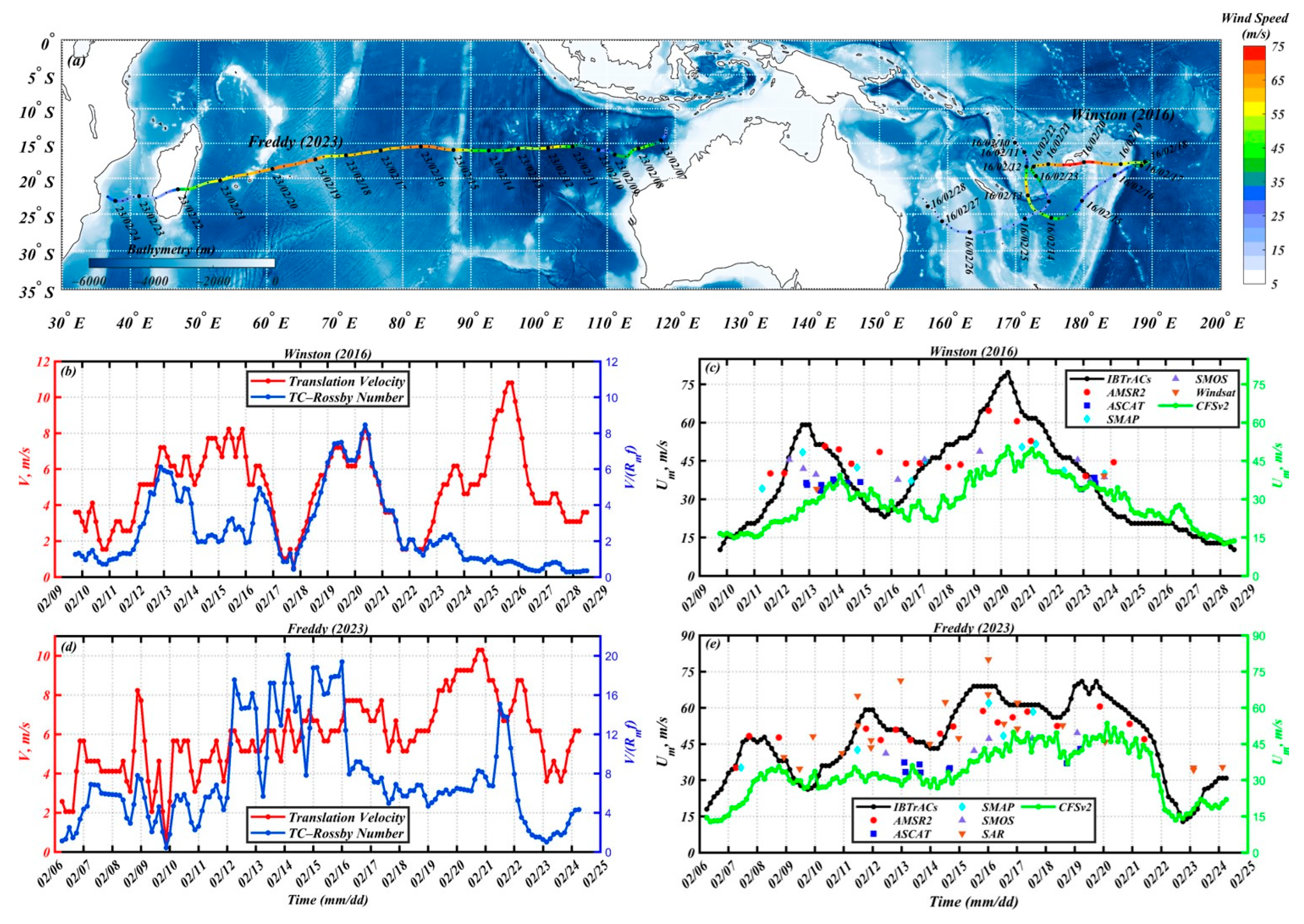
3.1. Brief Description of the Two TCs (Winston and Freddy)

The TC Winston was documented as one of the most destructive TCs in the Southern Hemisphere. It was generated at 18:00 UTC on 9 February 2016 and persisted for 20 days, featuring an atypical track characterized by a sudden change in direction and two distinct periods of rapid intensification (Figure 1a). The translation velocity (red line) and maximum sustained wind speed (black line) are shown in Figure 1b and Figure 1c, respectively. TC Winston first intensified to a Category-4 TC, with wind speeds reaching around 59.2 m/s. It then proceeded on a south-southeast trajectory at 6.2 m/s at 18:00 UTC on 12 February. After two days, Winston was located at 25°S, 177.5°E, and initiated a northeast movement at 6.6 m/s, accompanied by winds averaging 36 m/s. On 18 February, the maximum sustained winds of Winston reached 51.4 m/s as it traveled westward at a speed of 2.1 m/s. At the present moment, TC Winston continued to strengthen and reached a Category-5 status with a maximum sustained wind of 79.7 m/s at 6:00 UTC on 20 February. After making landfall over Fiji, Winston subsequently weakened and moved slowly southward at a speed of 2 m/s on 22 February. On 24 February, Winston encountered a strong vertical wind shear, which caused its winds to decrease to 25.7 m/s.

TC Freddy, which occurred over the southern tropical Indian Ocean in 2023, lasted for 35 days, making it the longest-lived TC on record on Earth. Figure 1a illustrates the lifespans of TC Freddy, while Figure 1d and Figure 1e present the time series of translation velocity and maximum sustained wind speed throughout its life cycle, respectively. It formed as a tropical storm with a wind speed of 18 m/s at 06:00 UTC on 6 February 2023 near 12.2°S, 118.6°E, intensifying to typhoon strength on 7 February. It subsequently moved in a west-southwest direction steadily, averaging 5.8 m/s. Later that day, Freddy transformed into a Category-2 TC, with the maximum sustained winds reaching 47.8 m/s. In the following several days (10–12 February), the storm gradually intensified to a Category-4 TC by 12 February, with peak winds reaching 59.2 m/s. At 6:00 UTC on 19 February, Freddy was located at 17°S, 65.7°E, and had reached Category-5 strength with a wind speed of 70.9 m/s. The storm quickly moved toward Madagascar at about 10 m/s, regained strength over the Mozambique Channel, made landfall in Mozambique, and dissipated at 12:00 UTC on 24 February. However, at 6:00 UTC on 2 March, the storm redeveloped over the Mozambique Channel and finally dissipated at 6:00 UTC on March 13 after making landfall (specific location not provided in the figure).

In addition, the TC Rossby number is often considered one of the key parameters to determine the influence of the storms on the upper ocean layers [59,60],

$$R_0=\frac{V}{R_{MW}f}$$

(1)

where $f$ is the Coriolis parameter, $V$ is the TC translation velocity, and $R_{MW}$ is the radius of maximum wind speed. If $R_0<1$, the TCs are defined as slow TCs. And if $R_0>1$, the TCs are defined as fast TCs. The Rossby numbers of the TC Winston displayed a wide range, varying from 0.3 to 8.5, as illustrated in Figure 1b. In contrast, the Rossby numbers ranged from 1.0 to 20.1 for the TC Freddy (Figure 1d). Variations in TC size can influence the Rossby number. The Rossby number shows an inverse relationship with the translation velocity trend for TC Winston after 23 February and for TC Freddy between 16 and 21 February, due to the notable increase in the TCs radius. Hence, TC Winston and Freddy were classified as fast-moving storms during most of their life span. During the period of 25–28 February 2016, Winston was classified as a weak, slow-moving TC because the Rossby number was less than 1 and the maximum sustained wind speed was below 21 m/s. The oceanic responses induced by fast TCs are weaker than those induced by slow TCs [61].

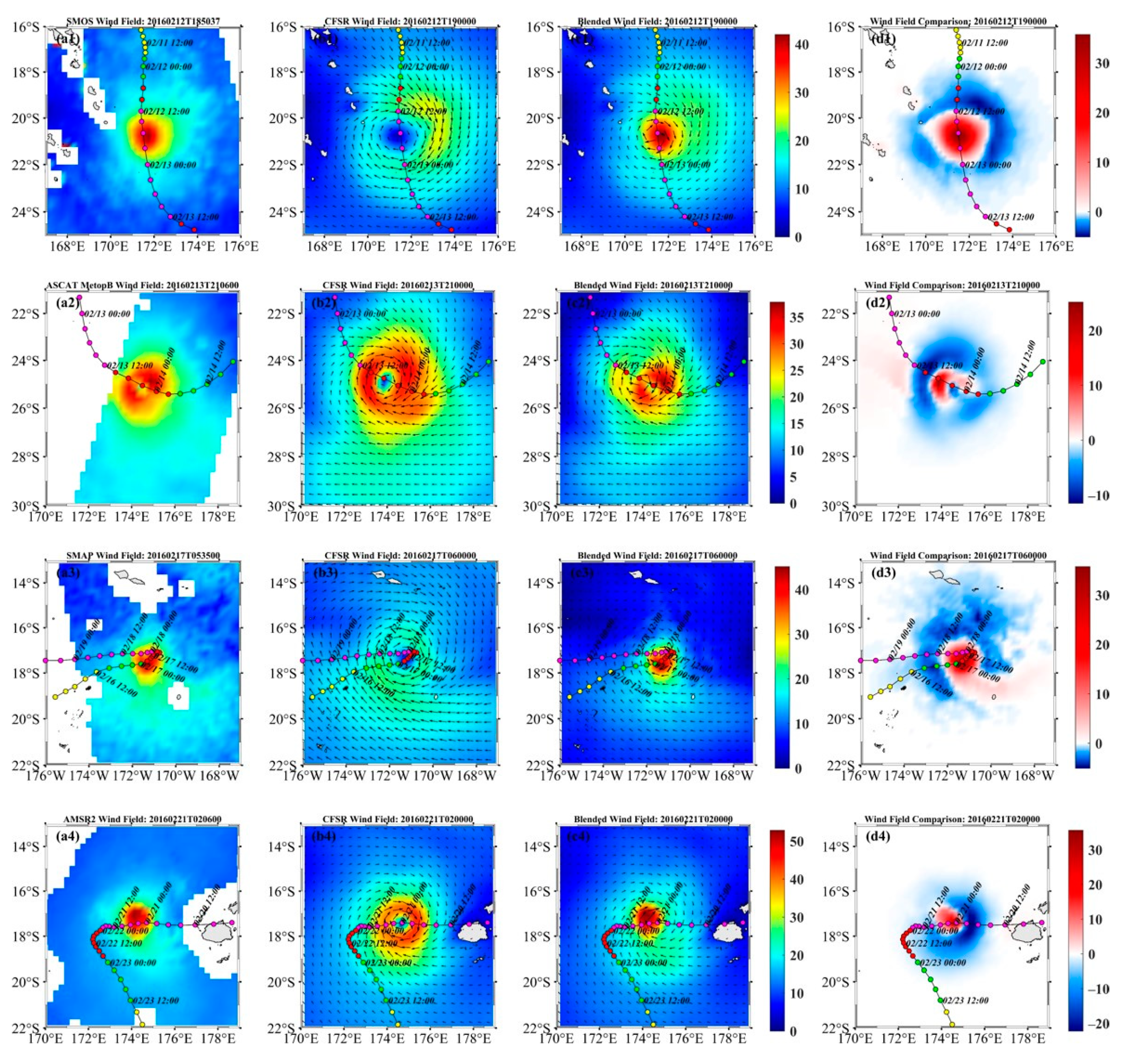
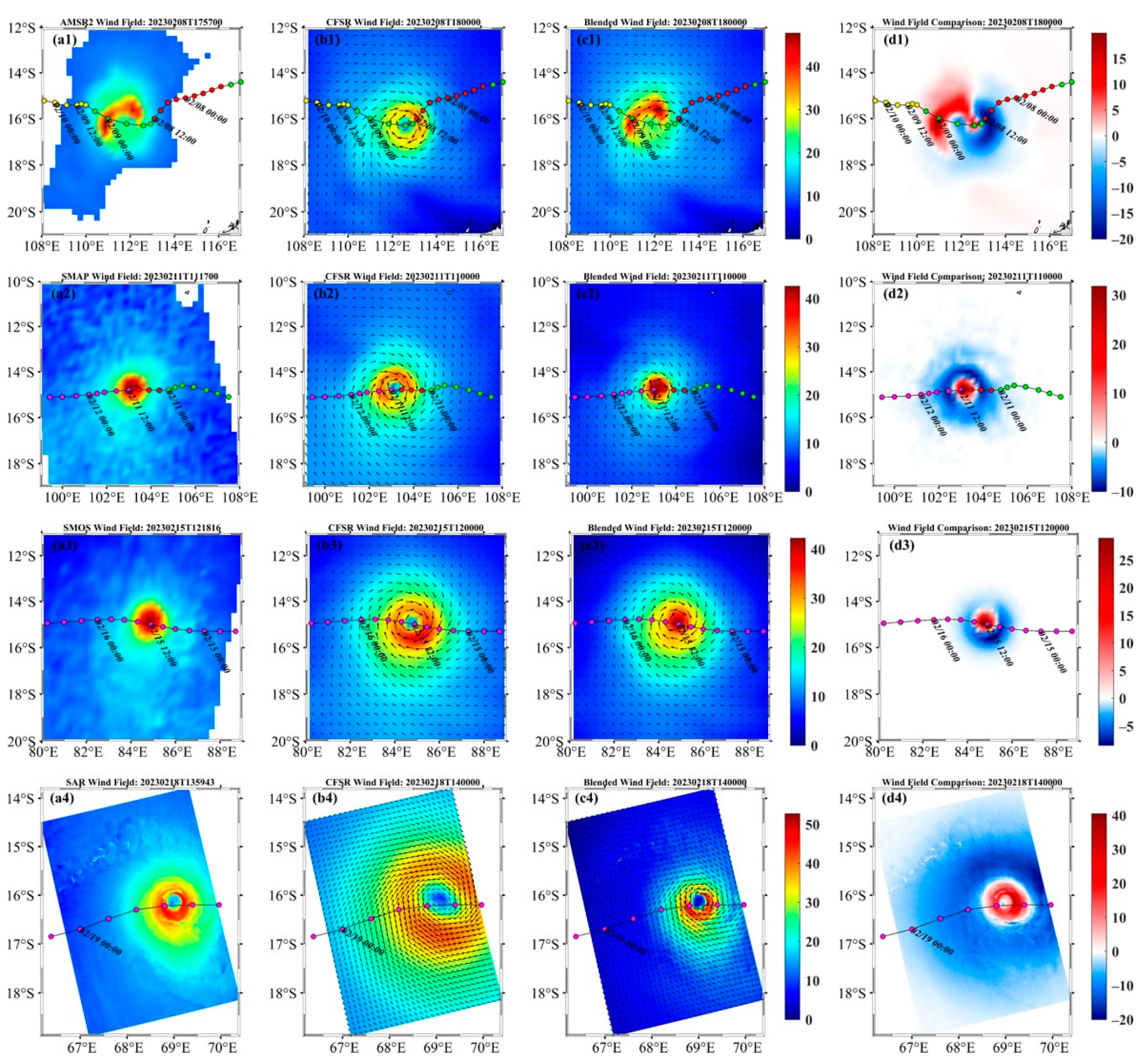
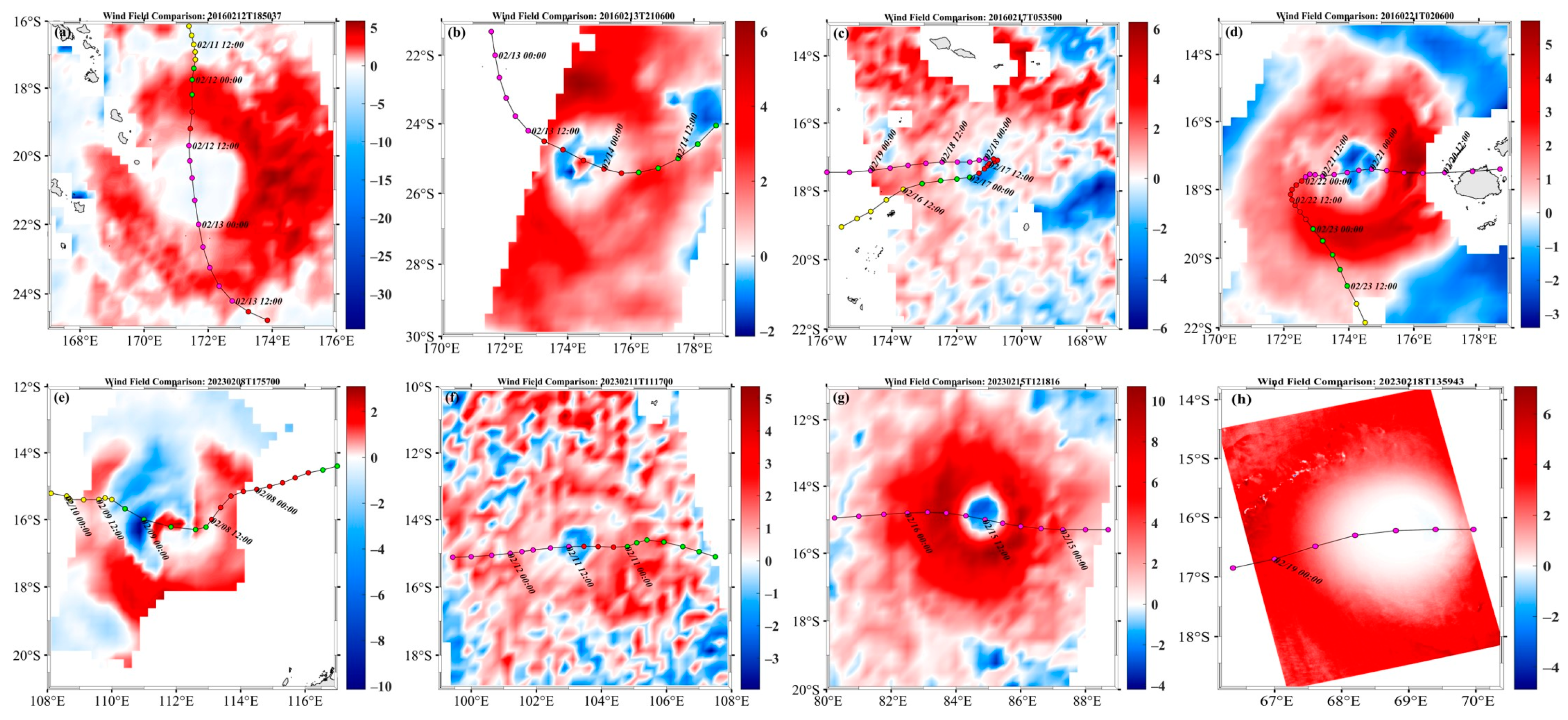
3.2. TC-Dedicated Blended Wind Fields

To improve the cyclone intensity in the ROMS model forcing, a combination of satellite winds from SMOS, SMAP, AMSR2, WindSat, ASCAT, SAR, and the CFSR winds were used to create the TC-dedicated blended wind fields. Figure 1c,e display the time series of maximum sustained surface wind speed along the track of the storms. The black line represents IBTrACS points, and the green line represents CFSR winds in Figure 1c,e. The temporal evolution of the peak wind speed provided by CFSR appears consistent with the best track data over the entire duration of the storm, whereas the CFSR winds do not capture the high winds of the storms. During TC Winston (2016) and Cyclone Freddy (2023), a total of 46 and 57 images of the sea surface wind fields were observed by multiple satellites, respectively (Figure 1c and Figure 1e). It was noted that the maximum wind speed along the track of the storms is higher than the CFSR winds. At 13:00 UTC on 19 February 2016, AMSR2 recorded a maximum wind speed of 64.7 m/s, while CFSR registered a maximum wind speed of only 38.1 m/s. In contrast to the maximum sustained wind speed provided by IBTrACS, the wind field observed by the AMSR2 satellite can more accurately depict the maximum wind speed of TC Winston (Figure 1c). To mitigate the underestimation of CFSR winds, a proposed approach involves using the wind field derived from the CFSR as the background field and overlaying it with the wind field generated by satellite winds.

To derive a blended wind field, the first step involves determining the consistent observation time between the satellite winds and the CFSR winds. Based on the observation time of satellite winds, CFSR winds with a temporal interval of less than 30 min are selected as the background wind field. The next step involves assessing whether the peak of the satellite winds reaches the critical TC wind speed of 33 m/s and comparing the maximum wind speeds of the satellite winds with those of the CFSR winds. This is carried out to ensure that the additional satellite winds optimize the underestimated wind speed of CFSR. The third step involves merging the satellite winds with the CFSR winds to obtain the blended product. To perform blending effectively, it is essential to determine the optimized distance for superimposition. Since two different wind field datasets (CFSR and satellite winds) are used, an abrupt switch of data at the optimized distance can lead to discontinuities in the wind fields. To achieve a smooth transition of the ocean surface wind field, a weighting coefficient is involved [62],

$$V_{new}=V_R\left(1-e\right)+e{V}_{CFSR}$$

(2)

where $V_R$ is the wind observed by remote sensing, and $V_{CFSR}$ is the wind from CFSR. The weight coefficient $e$ is calculated via

$$e=\frac{C^4}{1+C^4}$$

(3)

$$C=r/\left(n{R}_{MW}\right)$$

(4)

where $r$ is the radial distance between the TC center and the calculation grid point, and $R_{MW}$ is the radius of maximum wind speed. And the empirical parameter $n$ is set to be 9.

Improved fields are generated by incorporating satellite winds into the CFSR winds, as described above. As with the CFSR winds, the blended winds have a 0.2° spatial resolution and a 1 h temporal resolution. Figure 2 and Figure 3 illustrate the spatial distribution of the wind fields observed by satellites, CFSR winds, and blended winds during the four synoptic periods of TCs Winston and Freddy. The analysis indicates that the satellite winds are greater within the inner core area of TC Winston and Freddy compared to the CFSR winds. For CFSR winds, the maximum wind speeds along the track of the TC Winston are 25.5 m/s, 34.3 m/s, 22.9 m/s, and 44.9 m/s at 18:50 UTC on the 12, 21:06 UTC on the 13, 05:35 UTC on the 17, and 02:06 UTC on the 21 February 2016, respectively (Figure 2). Whereas for satellite winds, these values are 41.9 m/s, 37.8 m/s, 45.1 m/s, and 52.8 m/s (Figure 2). Similarly, the CFSR winds are underestimated by 4.6 m/s to 12.1 m/s for TC Freddy (2023). As illustrated in Figure 3, the maximum wind speeds of satellite winds are 47.71 m/s, 42.54 m/s, 42.24 m/s, and 52.70 m/s at 17:57 UTC on the 8, 11:17 UTC on the 11, 12:18 UTC on the 15, and 13:59 on the 18 February 2023, respectively. The maximum wind speeds of the blended winds have a closer alignment with the best track data compared to the CFSR winds (Figure 1e). Figure 2 and Figure 3 illustrate that the blended winds effectively show the high wind speeds along the tracks of TC Winston and Freddy. In contrast, the CFSR winds underestimate the high wind speed around the storm eye.

Figure 2(d1–d4) illustrates the difference between blended winds and the CFSR winds during the passage of TC Winston (2016). For TC Freddy (2023), the difference between the blended winds and the CFSR winds is depicted in Figure 3(d1–d4). The distribution of the blended winds maintains the asymmetric structure of TCs. The surface wind speeds within the inner core have significantly increased, with maximum changes reaching up to 38 m/s. Figure 4 shows the differences in wind speed between the blended winds and satellite winds during TCs Winston (2016) and Freddy (2023). The blended wind field aligns with satellite winds around the inner core and corresponds with the CFSR winds within the outer core region. At 18:00 UTC on 8 February 2023, the blended wind speed in the left rear quadrant is noticeably weaker than that of CFSR. This is because the storm center of CFSR was off by 70 km at that moment compared to the AMSR2 observation. Hence, a limitation of the blended surface vector winds is the presence of a storm center positional bias. This discrepancy arises from the relative shift of the cyclone center as observed between the satellite winds and the CFSR winds. The absence of wind direction data in the microwave radiometers (AMSR2, SMAP, and SMOS) necessitates the utilization of CFSR data to calculate wind direction in the blended sea surface vector winds.

3.3. Oceanic Temperature Response

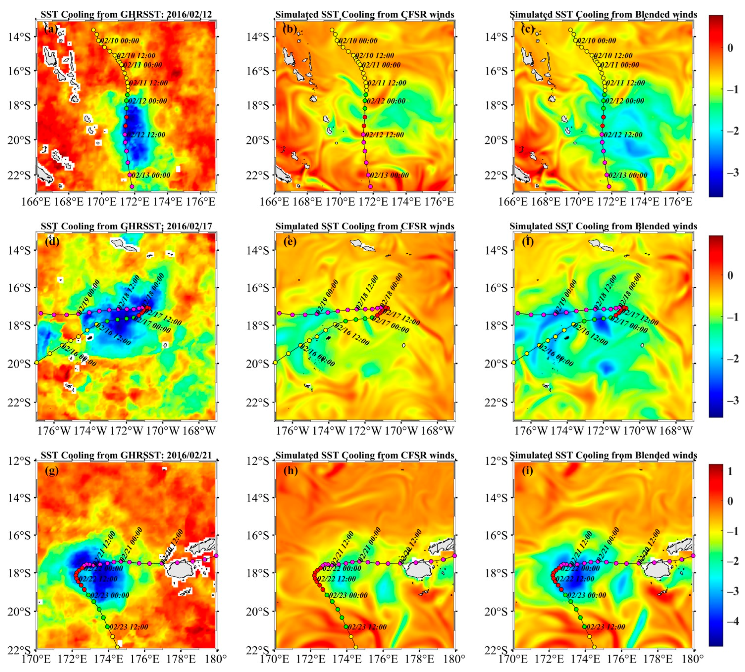
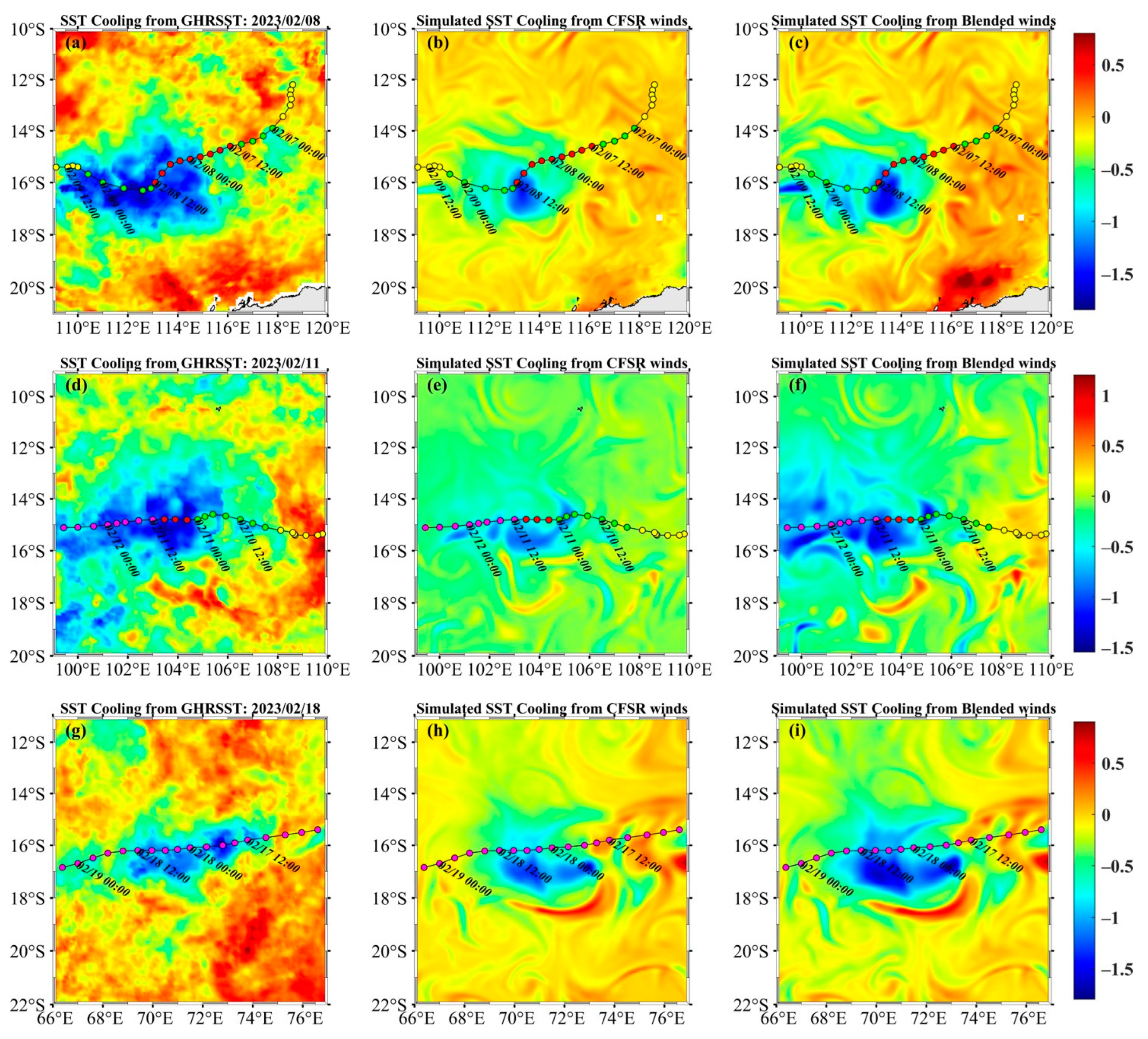
3.3.1. Sea Surface Cooling

To best evaluate the SST anomaly, we consider the SST difference ($∆SST$) between the day after TC passage ($t+1$) and one day before TC passage ($t-1$):

$$∆SST\left(t\right)=SST\left(t+1\right)-SST(t-1)$$

(5)

Figure 5 illustrates the SST anomalies during the passage of TC Winston on 12, 17, and 21 February 2016. The SST decreased on the left side of the track, while it remained almost unchanged on the right side. The generation of left (right)-biased SST wakes in the Southern (Northern) Hemisphere by the storms has been previously attributed to two phenomena [1]. Initially, the wind stress asymmetry associated with the storm’s translation speed can release more energy into the ocean on the left side of the track (Southern Hemisphere). Moreover, the interaction between wind and inertial currents on the same side can lead to enhanced vertical mixing [1,4,19].

The remote sensing detected significant decreases in SST with a minimum SST of 3.61 °C, 3.42 °C, and 4.85 °C on 12 February (Figure 5a), 17 February (Figure 5d), and 21 February (Figure 5g) 2016, respectively. These SST anomalies were also simulated by the ocean model (ROMS). On 12 February, ROMS-simulated SST changes forced by CFSR and the blended wind fields were −1.72 °C and −2.51 °C (Figure 5b,c), with a maximum SST decrease of 1.81 °C and 2.78 °C on 17 February (Figure 5e,f). Moreover, on 21 February, the modeled SST dropped by 2.85 °C and 4.36 °C, as predicted by CFSR and the blended wind fields (Figure 5h,i). Both of the simulated SST anomalies were slightly weaker than the observed ones. The values simulated by the blended wind fields were closer to the observed values than those simulated with CFSR wind fields. The maximum wind speed observed by satellite was higher (up to 22.2 m/s at 6:00 UTC on 17 February 2016) than that recorded by CFSR (Figure 2). This variation is likely due to the underestimated wind intensity in the CFSR dataset when compared to the satellite data.

Figure 6 illustrates the SST anomalies during the passage of TC Freddy on 8, 11, and 18 February 2023. Similar to the findings in TC Winston (2016), the SST cooling exhibits a slight leftward bias. By 8 February (Figure 6a), the GHRSST had decreased by approximately 1.84 °C after the passage of TC Freddy, showing a bias towards the left side of its track. At the same moment, the SST simulated by CFSR and the blended winds dropped by about 1.49 °C and 1.62 °C (Figure 6b,c). On 18 February, the maximum cooling in GHRSST is about 1.80 °C (Figure 6g). By contrast, it is about 1.52 °C and 1.76 °C, respectively, in the model forced by CFSR and blended winds, respectively (Figure 6h and Figure 6i). Both of the modeled SST anomalies were slightly weaker than the observed ones. The simulated SST using the blended wind fields was closer to the observations than when using CFSR wind fields. This difference is likely caused by the underestimated wind intensity from CFSR compared to the satellite observations.

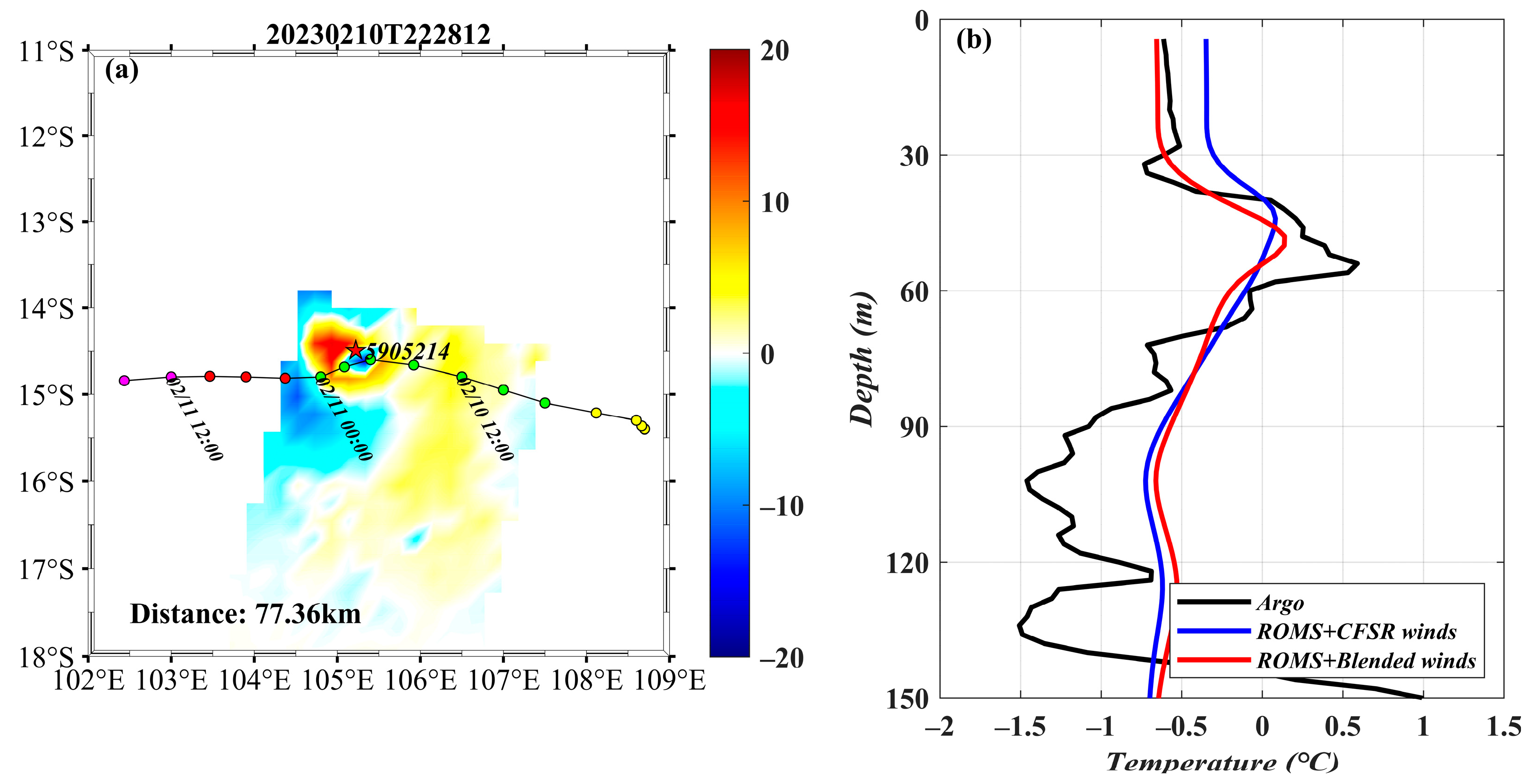
3.3.2. Subsurface Response

We investigated the subsurface temperature changes induced by TCs Winston (2016) and Freddy (2023) using data from Argo floats (Figure 7 and Figure 8). For Winston (2016), R5902145 was located on the right side of its track, R5904145 was near the center of Winston, and R5900953 was on the left side of its track. R5905214 was located on the right side of Freddy (2023). The distances between the Argo floats and the storm center were approximately 189.57 km, 42.75 km, 132.39 km, and 77.36 km, respectively.

We compared the vertical temperature differences measured by Argo from 0 m to 150 m deep with the simulated results from ROMS during the passage of TCs Winston and Freddy (Figure 7 and Figure 8). By comparing the wind fields recorded by CFSR and satellite data, it was found that the wind speeds differed significantly from those recorded by the Argo float (R5904145), showing a difference of 19.9 m/s at 12:40 UTC on 16 February 2016 (Figure 7c). It should be noted that we interpolate the simulated vertical temperatures to the vertical position of the Argo floats for comparison with the observational data. The near-surface temperature observed by the Argo buoy was 29.44 °C. In comparison, the simulated near-surface temperature forced by CFSR and the blended wind fields was 27.23 °C and 28.65 °C, respectively. These values were accompanied by wind speeds of 18.5 m/s and 38.4 m/s. Figure 7d shows a decrease of 0.1 °C to 1.2 °C in the temperature observed by Argo above 56 m on 16 February. Compared to the temperature changes measured by Argo, the model-simulated temperature forced by CFSR winds decreased by 0.1 °C to 0.8 °C, while those forced by the blended winds decreased by 0.1 °C to 1.0 °C. There was a clear differentiation of 0.2 °C in the upper 34 m layer between the simulation using CFSR winds and the blended winds. For R5902145 and R5900953, the simulated temperature differences from the blended winds decreased by 0.2 °C to 0.6 °C compared to those from the CFSR winds (Figure 7b,d). The wind speed of the blended winds at floats R5902145 and R5900953 is 3.05 m/s and 2.39 m/s less than those of CFSR, respectively. This may be related to the longer distance between the storm center and the Argo buoy’s location. The outer wind field of the storm in the blended winds still reflects the wind speed provided by CFSR winds. Compared to in situ observations, the simulated vertical temperature changes were underestimated when using both the CFSR winds and the blended winds to drive the ocean model. This is because the bias of the numerical simulation results is also influenced by factors such as the initial conditions of the ocean, the air–sea flux, and the vertical mixing parameterization.

At 22:28 UTC on 10 February 2023, the near-surface temperature was measured to be 28.40 °C. At the same time, the simulated near-surface temperature forced by CFSR winds was 27.01 °C, whereas that from the blended wind was 28.19 °C. Figure 8b depicts a similar vertical temperature change phenomenon for TC Winston. Figure 8b shows a decrease of 0.4 °C to 0.6 °C in the Argo-measured temperature above 38 m, a 0.1 °C to 0.5 °C increase between 40 m and 58 m, and a 0.1 °C to 1.5 °C decrease between 60 m and 144 m. The inclusion of satellite wind observations resulted in a simulated subsurface temperature profile forced by the blended wind field that aligns more closely with Argo observations.

We estimate the mixed layer depth (MLD) using a threshold of 0.8 °C temperature difference between the values at the 10 m depth and the base of the MLD [63]. Based on Argo’s observations during the impact of TC Winston, the MLD was 41.1 m on 16 February. The model under-predicted the observed MLD, which was 34.8 m and 36.4 m when simulated with CFSR and the blended wind fields, respectively. Figure 7 and Figure 8 demonstrate that the wind intensity of the blended wind fields closely approximated the satellite observations. Consequently, this led to a more accurate estimation of the simulated MLD, resulting in an improved vertical temperature simulation. This is due to the stronger surface winds, which lead to increased mixing and a deeper mixed layer. Moreover, the upper ocean response is controlled by mixing, advection, and air–sea flux (i.e., heat flux and freshwater flux). During the TC forcing stage, the mixing effect on temperature cooling is more significant than heat loss through air–sea flux. The responses of the upper ocean depend on the TCs intensity, translation speed, and size. Both the TCs Winston (2016) and Freddy (2023) were classified as fast-moving storms. The short residence time of fast-moving TCs in the upper ocean and the weak coupling between the wind stress and ocean inertial motions result in a negligible oceanic response within the mixed layer. Consequently, the improvement effect of numerical simulations below the mixed layer is limited.

To evaluate the precision of the numerical experiments driven by the blended winds, we calculated the correlation coefficient ($R^2$) and the root-mean-square difference ($RMSD$) between simulated and observed vertical temperature profiles [64].

$$R^2=\frac{{\sum }_{i=1}^N(V_{obs}-\overline{V_{obs}})(V_{model}-\overline{V_{model}})}{\sqrt{{\sum }_{i=1}^N{(V_{obs}-\overline{V_{obs}})}^2}\sqrt{{\sum }_{i=1}^N{(V_{model}-\overline{V_{model}})}^2}}$$

(6)

$$RMSD=\sqrt{\frac{1}{N}{\sum }_{i=1}^N{(V_{obs}-V_{model})}^2}$$

(7)

where $V_{obs}$ and $V_{model}$ is the observed and simulated temperature; N represents the total number of datasets used in the calculation. When comparing the temperature profiles at the four Argo locations, it is evident that the vertical temperature profiles simulated using the blended winds ($RMSD=0.81$ and $R^2=0.98$) have a significantly higher level of accuracy compared to those simulated using the CFSR wind field ($RMSD=2.13$ and $R^2=0.86$). We further utilize a skill score (SS) to objectively quantify the performance of numerical experiments conducted with the blend winds in comparison to simulations driven by CFSR winds. The skill scores ${SS}_r$ and ${SS}_c$ are given by:

$${SS}_r=1-\frac{RMSD\left(b\right)}{RMSD\left(c\right)}$$

(8)

$${SS}_c=\frac{R^2\left(b\right)}{R^2\left(c\right)}-1$$

(9)

where $b$ and $c$ are the experiment forced by the blended winds and the CFSR winds, respectively. If ${SS}_r>0$ when $RMSD\left(b\right)<RMSD\left(c\right)$ which means an improved simulation. For ${SS}_c>0$ when $R^2\left(b\right)>R^2\left(c\right)$, that is, a better model performance. The $R^2$, $RMSD$, ${SS}_r$, and ${SS}_r$ values computed from the individual criteria for the four Argo observational profiles are presented in

Table 1. Correlation coefficient ($R^2$), root-mean-square difference ($RMSD$), and skill score (${SS}_r$ and ${SS}_c$) for the vertical temperature.

Argo ID	$\mathit{R}\mathit{M}\mathit{S}\mathit{D}\left(\mathit{c}\right)$	${\mathit{R}}^2\left(\mathit{c}\right)$	$\mathit{R}\mathit{M}\mathit{S}\mathit{D}\left(\mathit{b}\right)$	${\mathit{R}}^2\left(\mathit{b}\right)$	${\mathit{S}\mathit{S}}_{\mathit{r}}$	${\mathit{S}\mathit{S}}_{\mathit{c}}$
R5902145	1.385	0.554	0.997	0.998	1.832	0.002
R5904145	1.379	0.972	0.594	0.987	1.785	0.016
R5900953	3.334	0.937	0.888	0.962	3.446	0.026
R5905214	2.459	0.992	0.750	0.997	2.709	0.006

. As we observed in the analyses above, improving the simulation of ocean temperatures can be achieved by optimizing the atmospheric wind forcing fields of the numerical model through the integration of multi-source satellite wind fields. Therefore, more accurate wind forcing during severe weather conditions results in enhanced mixing, thereby aligning the simulations more closely with observational data.

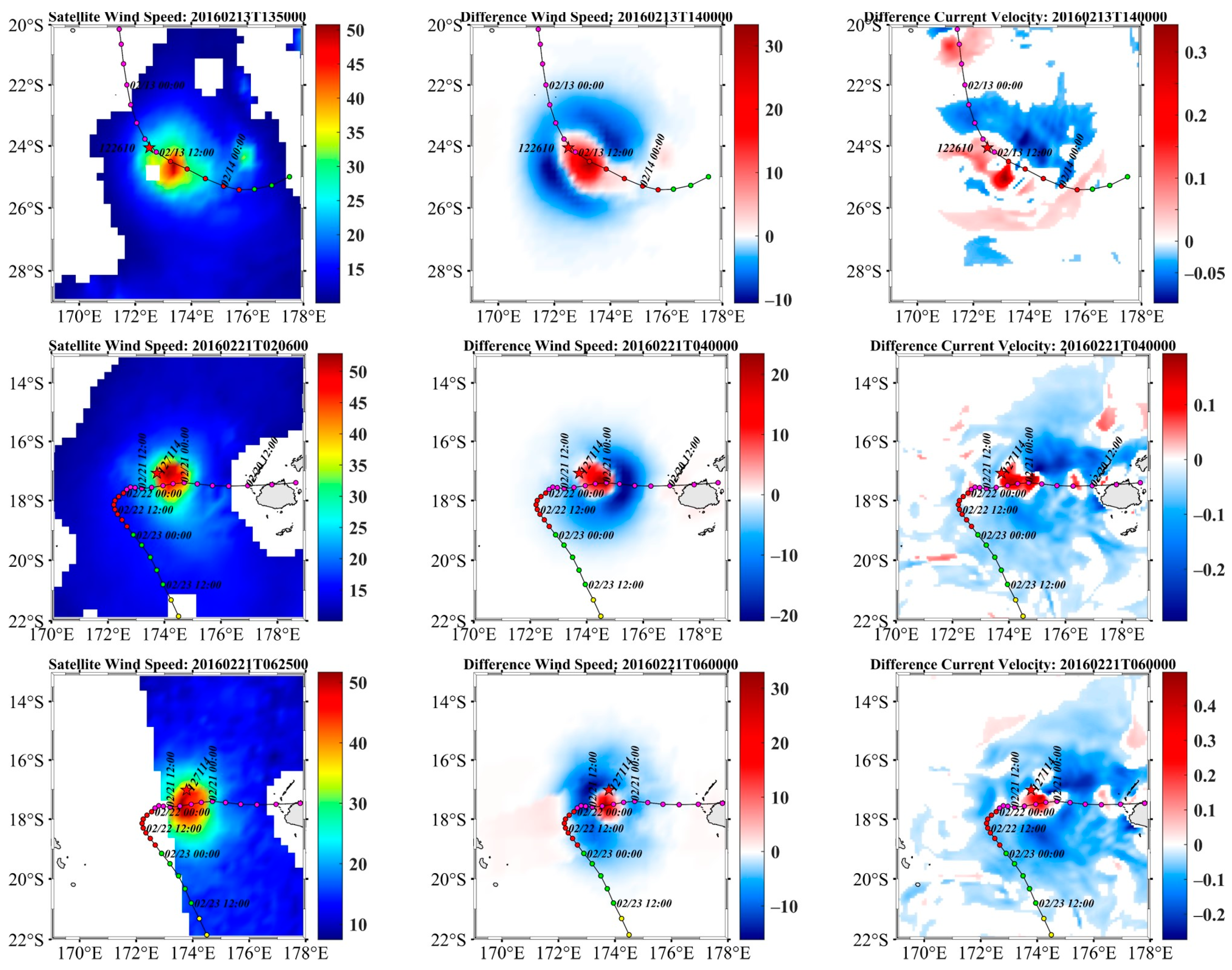
3.4. Near Surface Current Velocity Response

As a TC moves over the ocean, the strong wind stress induced by the storm leads to the modification of ocean currents, aligning the current direction with that of the wind forcing. There was a clear near-surface current response across the domain during TCs Winston (2016) and Freddy (2023) (Figure 9 and Figure 10). The first column of Figure 9 displays the satellite-observed wind fields at 13:50 UTC on the 13, at 02:06 UTC on the 21, and at 06:25 UTC on 21 February 2016, along with the differences in wind between CFSR winds and the blended winds provided in the second column (Figure 9). As the wind speed increased, the spatial distribution of the simulated surface current difference between CFSR winds and blended winds also exhibited an increase in current speed. The simulated surface current for Freddy (2023) agrees with that of Winston (2016).

It can be seen that there was a significant difference in wind speed within the 2° range of the TC center (Figure 10). We also compared the simulated ocean surface current velocities using two different wind-forcing fields to evaluate the impact of satellite winds on enhancing the simulation of current responses. The difference in simulated ocean current velocities corresponded to the difference in wind speeds, with the current responses being more pronounced at higher wind speeds. The near-surface currents are primarily influenced by wind stress. The resonance effect of the wind stress leads to the maximum current speed on the left side of the storm’s track. The difference between the observed and simulated currents may be due to the underestimation of the wind speed during high wind conditions.

In our study area, two surface drifter floats were collected from 9 to 28 February 2016. One of the floats (ID 122610) was 91.28 km from the storm center at 14:00 UTC on 13 February 2016, while the other one (ID 122612) was located at 72.19 km and 56.35 km from the storm center at 03:00 UTC on the 21 and at 06:00 UTC on 21 February 2016 (Figure 9). Near the center of TCs, winds play a crucial role in ocean thermodynamic and dynamic responses. However, the wind contribution weakens farther away from the center of TCs, as the ocean responses are mainly influenced by horizontal advection. The ocean 15 m current velocities observed by surface drifter floats were 1.40 m/s, 1.0 m/s, and 1.15 m/s at 14:00 UTC on the 13, at 03:00 UTC on the 21, and at 06:00 UTC on the 21 February 2016, respectively (

Table 2. The ocean current velocities and the corresponding wind speeds. (Units of current velocities and wind speeds are m/s).

UTC Time	${\mathit{W}}_{\mathbf{C}\mathbf{F}\mathbf{S}\mathbf{R}}$	${\mathit{W}}_{\mathbf{B}\mathbf{l}\mathbf{e}\mathbf{n}\mathbf{d}\mathbf{e}\mathbf{d}}$	${\mathit{U}}_{\mathbf{O}\mathbf{b}\mathbf{s}\mathbf{e}\mathbf{r}\mathbf{v}\mathbf{e}\mathbf{d}}$	${\mathit{U}}_{\mathbf{S}\mathbf{i}\mathbf{m}\mathbf{u}\mathbf{l}\mathbf{a}\mathbf{t}\mathbf{e}\mathbf{d}\_\mathbf{C}\mathbf{F}\mathbf{S}\mathbf{R}}$	${\mathit{U}}_{\mathbf{S}\mathbf{i}\mathbf{m}\mathbf{u}\mathbf{l}\mathbf{a}\mathbf{t}\mathbf{e}\mathbf{d}\_\mathbf{B}\mathbf{l}\mathbf{e}\mathbf{n}\mathbf{d}\mathbf{e}\mathbf{d}}$
2016-02-13 14:00	19.55	26.41	1.40	0.54	0.62
2016-02-21 03:00	39.21	45.85	1.00	0.71	0.81
2016-02-21 06:00	37.07	44.99	1.15	0.64	0.75
2023-02-11 12:00	22.22	17.21	0.52	0.23	0.18
2023-02-12 00:00	25.61	28.34	0.91	0.56	0.64

). The current velocity differences between observed and modeled velocities are 0.86 m/s, 0.29 m/s, and 0.51 m/s at 14:00 UTC on the 13, at 03:00 UTC on the 21, and at 06:00 UTC on the 21 February 2016 using the CFSR wind forcing, respectively. These values change to 0.78 m/s, 0.19 m/s, and 0.4 m/s when using the blended wind forcing.

For TC Freddy (2023), the two surface drifter floats were located at 135.5 km and 83.18 km from the storm center at 12:00 UTC and 23:00 UTC on 11 February 2023, respectively (see Figure 10). Similarly, the simulated surface current is smaller than the observed currents. At 12:00 on 11 February, the simulated current forced by CFSR winds was significantly larger than the simulated current forced by the blended winds. This is because the wind speed in CFSR is higher than the wind speed in blended winds. The simulated current velocities were underestimated at all times, and that is likely due to the absence of wave–current interaction processes in the ocean model. Among these, the TC-induced Stokes drift has a significant impact on the near-surface ocean current response.

In order to examine the impact of wind forcing on ocean current responses under TC forcing, the Stokes drift (${\mathbf{u}}_{\mathit{s}}$) is calculated as [65],

$${\mathbf{u}}_{\mathit{s}}\left(\mathit{z}\right)=0.04\mathit{U}exp\left[-\frac{4\sqrt{g\left|z\right|}}{W}\right]$$

(10)

where $\mathit{U}$ is the vector wind fields, $W$ is the scalar wind fields. The adjusted near-surface ocean current velocities, supplemented by Stokes drift, are provided in

Table 3. The observed and adjusted simulated ocean current velocities and the calculated Stokes drift using Equation (10) (Unit of the velocities: m/s).

UTC Time	${\mathit{U}}_{\mathbf{O}\mathbf{b}\mathbf{s}\mathbf{e}\mathbf{r}\mathbf{v}\mathbf{e}\mathbf{d}}$	${\mathit{U}}_{\mathbf{S}\mathbf{i}\mathbf{m}\mathbf{u}\mathbf{l}\mathbf{a}\mathbf{t}\mathbf{e}\mathbf{d}\_\mathbf{C}\mathbf{F}\mathbf{S}\mathbf{R}}$	${\mathit{U}}_{\mathbf{S}\mathbf{i}\mathbf{m}\mathbf{u}\mathbf{l}\mathbf{a}\mathbf{t}\mathbf{e}\mathbf{d}\_\mathbf{B}\mathbf{l}\mathbf{e}\mathbf{n}\mathbf{d}\mathbf{e}\mathbf{d}}$	${\mathbf{u}}_{\mathbf{s}\_\mathbf{C}\mathbf{F}\mathbf{S}\mathbf{R}}$	${\mathbf{u}}_{\mathbf{s}\_\mathbf{B}\mathbf{l}\mathbf{e}\mathbf{n}\mathbf{d}\mathbf{e}\mathbf{d}}$
2016-02-13 14:00	1.40	0.58	0.71	0.03	0.09
2016-02-21 03:00	1.00	1.03	1.27	0.31	0.46
2016-02-21 06:00	1.15	0.91	1.19	0.27	0.44
2023-02-11 12:00	0.52	0.33	0.22	0.10	0.04
2023-02-12 00:00	0.91	0.71	0.84	0.15	0.20

. After accounting for the Stokes drift, the simulated currents more closely resemble the observed surface currents. Compared with the sea surface velocity observed by surface drifting buoys, the sea surface velocity simulated by incorporating the satellite observations is closer to the observed value. Therefore, the simulated near-surface ocean current velocities quantitatively verify that the optimized wind forcing plays a significant role in the numerical simulation of the upper ocean responses.

4. Conclusions

We investigated the impact of satellite winds on numerical simulations based on multi-satellite observations, in situ measurements, and a 3D ocean circulation model (ROMS). The blended winds were generated by combining the surface winds observed by active and passive satellite-based microwave sensors with the CFSR analysis winds. By comparing observations with simulations, we confirmed that incorporating optimal TC wind forcing from satellite observations partially improved the accuracy of numerical simulations.

The blended winds can resolve high winds in and around TCs, which is a crucial feature for improving the simulations and predictions of the TC-ocean interaction. The reanalysis wind product, such as CFSR, is unable to accurately depict the high wind values along the storm tracks. The multi-satellite scatterometers and radiometers demonstrate a high sensitivity to strong winds and are not affected by rain attenuation. As a result, they provide precise wind measurements during severe storms. For instance, according to the IBTrACS best track data, the maximum sustained wind speed of Winston was 74.5 m/s on 19 February 2016. At the same time, AMSR2 recorded a maximum wind speed of 64.7 m/s, while the maximum wind speed of the CFSR winds was only 38.1 m/s. Comparisons with the best track data show that the satellite winds outperform the CFSR winds. Therefore, combining the multi-source satellite wind data with reanalysis winds can improve the wind forcing of numerical models.

The maximum amplitude of the SST decrease was 4.85 °C for Winston on 21 February 2016. However, the ROMS-simulated SST dropped by 2.85 °C and 4.36 °C when using wind forcing from CFSR alone and blended winds, respectively. Regarding TC Freddy (2023), both of the modeled SST anomalies were slightly weaker than the observed ones. The stronger surface winds can enhance vertical mixing, bringing cooler, deeper water to the surface, which results in a decrease in the sea surface temperature. In addition, the primary reason for the differences between the simulated SST of the two experiments is the underestimation of wind intensity at extreme wind speeds (up to ~55 m/s) by CFSR compared to the satellite observations.

Both the vertical temperature profiles and MLD showed that the TC blended wind forcing resulted in more accurate thermal responses than the CFSR winds. The Argo-measured mixed layer depth was 41.1 m on the right side of the storm track, whereas the MLD was 34.8 m and 36.4 m simulated by CFSR alone and the blended winds on 16 February 2016. Analyzing the vertical temperature profiles, the simulation using blended winds performs best in terms of the skill score (SS). Among the simulated vertical temperatures, the RMSD and $R^2$ of the blended wind forcing experiment were 0.81 and 0.98, respectively. The higher RMSD and the lower values of $R^2$ of the CFSR wind forcing experiment were 2.13 and 0.86, respectively. This suggests that the accuracy of ocean temperature simulation could be improved by optimizing the atmospheric wind forcing fields of the numerical model through the integration of multi-source satellite wind data.

Consistent with the ocean temperature, a similar phenomenon was observed with oceanic currents. We quantitatively compared the measured current by surface drifters with the current simulated by ROMS using two different wind field inputs. The ocean current velocities observed by surface drifter floats were 1.40 m/s, 1.15 m/s, and 0.91 m/s at 14:00 UTC on the 13, at 06:00 UTC on the 21 February 2016, and at 00:00 UTC on 12 February 2023, respectively. The differences in current velocity between observed and simulated data were 0.86 m/s, 0.29 m/s, and 0.51 m/s when using wind forcing from the CFSR alone. Corresponding variances of 0.78 m/s, 0.19 m/s, and 0.4 m/s were simulated when using wind forcing from the blended winds. The impact of wind forcing on the upper ocean responses to TCs in numerical simulations was further confirmed. In general, the blended model can effectively simulate the storm wind fields. Therefore, the numerical simulations of upper ocean responses to TCs based on the blended winds are more accurate.

With the development of satellite constellations, the temporal and spatial resolution of oceanic observations are gradually increasing. Spaceborne synthetic aperture radars, radiometers, and scatterometers can provide high spatial resolution and high temporal resolution of ocean surface wind fields even under extreme weather conditions. These active and passive sensors can improve the wind forcing and ocean modeling of the upper ocean response to TCs. Nevertheless, numerical simulations are also affected by other factors. To improve the overall accuracy of model predictions, it is possible to integrate atmospheric, oceanic, and wave models to study the overall oceanic responses and dynamic processes. Moreover, contributions to the TCs from the impacts of improved drag formulations and dissipative heating are potentially problematic. However, these aspects are not within the scope of this study and are reserved for future investigations.

References

1. Price, J.F. Upper Ocean Response to a Hurricane. J. Phys. Oceanogr. 1981, 11, 153–175. [Google Scholar] [CrossRef]
2. Bender, M.A.; Ginis, I.; Kurihara, Y. Numerical simulations of tropical cyclone-ocean interaction with a high-resolution coupled model. J. Geophys. Res. Atmos. 1993, 98, 23245–23263. [Google Scholar] [CrossRef]
3. Bender, M.A.; Ginis, I. Real-Case Simulations of Hurricane–Ocean Interaction Using a High-Resolution Coupled Model: Effects on Hurricane Intensity. Mon. Weather Rev. 2000, 128, 917–946. [Google Scholar] [CrossRef]
4. Sanford, T.B.; Price, J.F.; Girton, J.B.; Webb, D.C. Highly resolved observations and simulations of the ocean response to a hurricane. Geophys. Res. Lett. 2007, 34, L13604. [Google Scholar] [CrossRef]
5. Halliwell, G.R.; Shay, L.K.; Jacob, S.D.; Smedstad, O.M.; Uhlhorn, E.W. Improving Ocean Model Initialization for Coupled Tropical Cyclone Forecast Models Using GODAE Nowcasts. Mon. Weather Rev. 2008, 136, 2576–2591. [Google Scholar] [CrossRef]
6. Halliwell, G.R.; Shay, L.K.; Brewster, J.K.; Teague, W.J. Evaluation and Sensitivity Analysis of an Ocean Model Response to Hurricane Ivan. Mon. Weather Rev. 2011, 139, 921–945. [Google Scholar] [CrossRef]
7. Morey, S.L.; Bourassa, M.A.; Davis, X.J.; O’Brien, J.J.; Zavala-Hidalgo, J. Remotely sensed winds for episodic forcing of ocean models. J. Geophys. Res. Ocean. 2005, 110, C10024. [Google Scholar] [CrossRef]
8. Prasad, T.G.; Hogan, P.J. Upper-ocean response to Hurricane Ivan in a 1/25° nested Gulf of Mexico HYCOM. J. Geophys. Res. 2007, 112, C04013. [Google Scholar] [CrossRef]
9. Seroka, G.; Miles, T.; Xu, Y.; Kohut, J.; Schofield, O.; Glenn, S. Rapid shelf-wide cooling response of a stratified coastal ocean to hurricanes. J. Geophys. Res. Ocean. 2017, 122, 4845–4867. [Google Scholar] [CrossRef]
10. Kistler, R.; Kalnay, E.; Collins, W.; Saha, S.; White, G.; Woollen, J.; Chelliah, M.; Ebisuzaki, W.; Kanamitsu, M.; Kousky, V.; et al. The NCEP-NCAR 50-Year Reanalysis: Monthly Means CD-ROM and Documentation. Bull. Am. Meteorol. Soc. 2001, 82, 247–267. [Google Scholar] [CrossRef]
11. Saha, S.; Moorthi, S.; Pan, H.L.; Wu, X.; Wang, J.; Nadiga, S.; Tripp, P.; Kistler, R.; Woollen, J.; Behringer, D.; et al. The NCEP Climate Forecast System Reanalysis. Bull. Am. Meteorol. Soc. 2010, 91, 1015–1058. [Google Scholar] [CrossRef]
12. Uppala, S.M.; KÅllberg, P.W.; Simmons, A.J.; Andrae, U.; Bechtold, V.D.C.; Fiorino, M.; Gibson, J.K.; Haseler, J.; Hernandez, A.; Kelly, G.A.; et al. The ERA-40 re-analysis. Q. J. R. Meteorol. Soc. 2005, 131, 2961–3012. [Google Scholar] [CrossRef]
13. Kiss, P.; Jánosi, I.M. Comprehensive empirical analysis of ERA-40 surface wind speed distribution over Europe. Energy Convers. Manag. 2008, 49, 2142–2151. [Google Scholar] [CrossRef]
14. Schenkel, B.A.; Lin, N.; Chavas, D.; Oppenheimer, M.; Brammer, A. Evaluating Outer Tropical Cyclone Size in Reanalysis Datasets Using QuikSCAT Data. J. Clim. 2017, 30, 8745–8762. [Google Scholar] [CrossRef]
15. Signell, R.P.; Carniel, S.; Cavaleri, L.; Chiggiato, J.; Doyle, J.D.; Pullen, J.; Sclavo, M. Assessment of Wind Quality for Oceanographic Modelling in Semi-Enclosed Basins. J. Mar. Syst. 2005, 53, 217–233. [Google Scholar] [CrossRef]
16. Wakelin, S.; Proctor, R. The impact of meteorology on modelling storm surges in the Adriatic Sea. Glob. Planet. Chang. 2002, 34, 97–119. [Google Scholar] [CrossRef]
17. Hodur, R.M. The Naval Research Laboratory’s Coupled Ocean/Atmosphere Mesoscale Prediction System (COAMPS). Mon. Weather Rev. 1997, 125, 1414–1430. [Google Scholar] [CrossRef]
18. Powell, M.D.; Houston, S.H.; Amat, L.R.; Morisseau-Leroy, N. The HRD real-time hurricane wind analysis system. J. Wind Eng. Ind. Aerodyn. 1998, 77–78, 53–64. [Google Scholar] [CrossRef]
19. Price, J.F.; Sanford, T.B.; Forristall, G.Z. Forced Stage Response to a Moving Hurricane. J. Phys. Oceanogr. 1994, 24, 233–260. [Google Scholar] [CrossRef]
20. Holland, G.J. An Analytic Model of the Wind and Pressure Profiles in Hurricanes. Mon. Weather Rev. 1980, 108, 1212–1218. [Google Scholar] [CrossRef]
21. Holland, G. A Revised Hurricane Pressure-Wind Model. Mon. Weather Rev. 2008, 136, 3432–3445. [Google Scholar] [CrossRef]
22. Holland, G.J.; Belanger, J.I.; Fritz, A. A Revised Model for Radial Profiles of Hurricane Winds. Mon. Weather Rev. 2010, 138, 4393–4401. [Google Scholar] [CrossRef]
23. Uhlhorn, E.W.; Klotz, B.W.; Vukicevic, T.; Reasor, P.D.; Rogers, R.F. Observed Hurricane Wind Speed Asymmetries and Relationships to Motion and Environmental Shear. Mon. Weather Rev. 2014, 142, 1290–1311. [Google Scholar] [CrossRef]
24. Olfateh, M.; Callaghan, D.P.; Nielsen, P.; Baldock, T.E. Tropical cyclone wind field asymmetry-Development and evaluation of a new parametric model. J. Geophys. Res. Ocean. 2017, 122, 458–469. [Google Scholar] [CrossRef]
25. Willoughby, H.E.; Rahn, M.E. Parametric Representation of the Primary Hurricane Vortex. Part I: Observations and Evaluation of the Holland (1980) Model. Mon. Weather Rev. 2004, 132, 3033–3048. [Google Scholar] [CrossRef]
26. Landsea, C.W.; Franklin, J.L. Atlantic Hurricane Database Uncertainty and Presentation of a New Database Format. Mon. Weather Rev. 2013, 141, 3576–3592. [Google Scholar] [CrossRef]
27. Murty, P.L.N.; Bhaskaran, P.K.; Gayathri, R.; Sahoo, B.; Kumar, T.S.; SubbaReddy, B. Numerical study of coastal hydrodynamics using a coupled model for Hudhud cyclone in the Bay of Bengal. Estuar. Coast. Shelf Sci. 2016, 183, 13–27. [Google Scholar] [CrossRef]
28. Murty, P.L.N.; Srinivas, K.S.; Rao, E.P.R.; Bhaskaran, P.K.; Shenoi, S.S.C.; Padmanabham, J. Improved cyclonic wind fields over the Bay of Bengal and their application in storm surge and wave computations. Appl. Ocean Res. 2020, 95, 102048. [Google Scholar] [CrossRef]
29. Shao, Z.; Liang, B.; Li, H.; Wu, G.; Wu, Z. Blended wind fields for wave modeling of tropical cyclones in the South China Sea and East China Sea. Appl. Ocean Res. 2018, 71, 20–33. [Google Scholar] [CrossRef]
30. Pan, Y.; Chen, Y.; Li, J.; Ding, X. Improvement of wind field hindcasts for tropical cyclones. Water Sci. Eng. 2016, 9, 58–66. [Google Scholar] [CrossRef]
31. McConochie, J.D.; Hardy, T.A.; Mason, L.B. Modelling tropical cyclone over-water wind and pressure fields. Ocean Eng. 2004, 31, 1757–1782. [Google Scholar] [CrossRef]
32. Rayson, M.D.; Ivey, G.N.; Jones, N.L.; Lowe, R.J.; Wake, G.W.; McConochie, J.D. Near-inertial ocean response to tropical cyclone forcing on the Australian North-West Shelf. J. Geophys. Res. Ocean. 2015, 120, 7722–7751. [Google Scholar] [CrossRef]
33. Wei, J.; Liu, X.; Wang, D.X. Dynamic and thermal responses of the Kuroshio to typhoon Megi (2004). Geophys. Res. Lett. 2014, 41, 8495–8502. [Google Scholar] [CrossRef]
34. Yin, X.; Wang, Z.; Liu, Y.; Xu, Y. Ocean response to Typhoon Ketsana traveling over the northwest Pacific and a numerical model spproach. Geophys. Res. Lett. 2007, 34, L21606. [Google Scholar] [CrossRef]
35. Brennan, M.J.; Hennon, C.C.; Knabb, R.D. The Operational Use of QuikSCAT Ocean Surface Vector Winds at the National Hurricane Center. Weather Forecast. 2009, 24, 621–645. [Google Scholar] [CrossRef]
36. Draper, D.W.; Long, D.G. Evaluating the effect of rain on SeaWinds scatterometer measurements. J. Geophys. Res. Ocean. 2004, 109, C02005. [Google Scholar] [CrossRef]
37. Reul, N.; Tenerelli, J.; Chapron, B.; Vandemark, D.; Quilfen, Y.; Kerr, Y. SMOS satellite L-band radiometer: A new capability for ocean surface remote sensing in hurricanes. J. Geophys. Res. Ocean. 2012, 117, C02006. [Google Scholar] [CrossRef]
38. Yueh, S.H.; Fore, A.G.; Tang, W.; Hayashi, A.; Stiles, B.; Reul, N.; Weng, Y.; Zhang, F. SMAP L-Band Passive Microwave Observations of Ocean Surface Wind During Severe Storms. IEEE Trans. Geosci. Remote Sens. 2016, 54, 7339–7350. [Google Scholar] [CrossRef]
39. Meissner, T.; Ricciardulli, L.; Wentz, F.J. Capability of the SMAP Mission to Measure Ocean Surface Winds in Storms. Bull. Am. Meteorol. Soc. 2017, 98, 1660–1677. [Google Scholar] [CrossRef]
40. Knapp, K.R.; Kruk, M.C.; Levinson, D.H.; Diamond, H.J.; Neumann, C.J. The International Best Track Archive for Climate Stewardship (IBTrACS): Unifying Tropical Cyclone Data. Bull. Am. Meteorol. Soc. 2010, 91, 363–376. [Google Scholar] [CrossRef]
41. GHRSST Project Office; Helen, B.; Ioanna, K.; Sandra, C. Sea Surface Temperature: An introduction to Users on the Set of GHRSST Products (1/2023); Zenodo: Geneva, Switzerland, 2023. [Google Scholar] [CrossRef]
42. Gaiser, P.W.; St Germain, K.M.; Twarog, E.M.; Poe, G.A.; Purdy, W.; Richardson, D.; Grossman, W.; Jones, W.L.; Spencer, D.; Golba, G.; et al. The WindSat spaceborne polarimetric microwave radiometer: Sensor description and early orbit performance. IEEE Trans. Geosci. Remote Sens. 2004, 42, 2347–2361. [Google Scholar] [CrossRef]
43. Meissner, T.; Ricciardulli, L.; Manaster, A. Tropical Cyclone Wind Speeds from WindSat, AMSR and SMAP: Algorithm Development and Testing. Remote Sens. 2021, 13, 1641. [Google Scholar] [CrossRef]
44. Ricciardulli, L.; Manaster, A. Intercalibration of ASCAT Scatterometer Winds from MetOp-A, -B, and -C, for a Stable Climate Data Record. Remote Sens. 2021, 13, 3678. [Google Scholar] [CrossRef]
45. Entekhabi, D.; Yueh, S.; O’Neill, P.E.; Kellogg, K.H.; Allen, A.; Bindlish, R.; Brown, M.; Chan, S.; Colliander, A.; Crow, W.; et al. SMAP Handbook. National Aeronautics and Space Administration. 2014; p. 192. Available online: https://smap.jpl.nasa.gov/mission/description/ (accessed on 4 December 2023).
46. Fernandez, D.E.; Carswell, J.R.; Frasier, S.; Chang, P.S.; Black, P.G.; Marks, F.D. Dual-polarized C- and Ku-band ocean backscatter response to hurricane-force winds. J. Geophys. Res. Oceans 2006, 111, C08013. [Google Scholar] [CrossRef]
47. Sapp, J.W.; Alsweiss, S.O.; Jelenak, Z.; Chang, P.S.; Frasier, S.J.; Carswell, J. Airborne Co-polarization and Cross-Polarization Observations of the Ocean-Surface NRCS at C-Band. IEEE Trans. Geosci. Remote Sens. 2016, 54, 5975–5992. [Google Scholar] [CrossRef]
48. Mouche, A.A.; Chapron, B.; Zhang, B.; Husson, R. Combined Co- and Cross-Polarized SAR Measurements Under Extreme Wind Conditions. IEEE Trans. Geosci. Remote Sens. 2017, 55, 6746–6755. [Google Scholar] [CrossRef]
49. Chandra, A.; Kumar, S. Sea Surface Temperature and Ocean Heat Content during Tropical Cyclones Pam (2015) and Winston (2016) in the Southwest Pacific Region. Mon. Weather Rev. 2021, 149, 1173–1187. [Google Scholar] [CrossRef]
50. Wang, Y.; Liu, Q.; Ma, Y. Upper Ocean Response to Typhoon Megi (2010). IOP Conf. Ser. Earth Environ. Sci. 2017, 52, 012063. [Google Scholar] [CrossRef]
51. Elipot, S.; Lumpkin, R.; Perez, R.C.; Lilly, J.M.; Early, J.J.; Sykulski, A.M. A global surface drifter data set at hourly resolution. J. Geophys. Res. Ocean. 2016, 121, 2937–2966. [Google Scholar] [CrossRef]
52. Lumpkin, R.; Pazos, M. Measuring surface currents with Surface Velocity Program drifters: The instrument, its data, and some recent results. In Lagrangian Analysis and Prediction of Coastal and Ocean Dynamics; Cambridge University Press: Cambridge, UK, 2007; pp. 39–67. [Google Scholar]
53. Shchepetkin, A.F.; McWilliams, J.C. The regional oceanic modeling system (ROMS): A split-explicit, free-surface, topography-following-coordinate oceanic model. Ocean Model. 2005, 9, 347–404. [Google Scholar] [CrossRef]
54. Fairall, C.W.; Bradley, E.F.; Hare, J.E.; Grachev, A.A.; Edson, J.B. Bulk Parameterization of Air–Sea Fluxes: Updates and Verification for the COARE Algorithm. J. Clim. 2003, 16, 571–591. [Google Scholar] [CrossRef]
55. Umlauf, L.; Burchard, H. A generic length-scale equation for geophysical turbulence models. J. Mar. Res. 2003, 61, 235–265. [Google Scholar] [CrossRef]
56. Umlauf, L.; Burchard, H.; Hutter, K. Extending the k − ω turbulence model towards oceanic applications. Ocean Model. 2003, 5, 195–218. [Google Scholar] [CrossRef]
57. Robertson, R.; Hartlipp, P. Surface wind mixing in the Regional Ocean Modeling System (ROMS). Geosci. Lett. 2017, 4, 24. [Google Scholar] [CrossRef] [PubMed]
58. Chassignet, E.P.; Hurlburt, H.E.; Smedstad, O.M.; Halliwell, G.R.; Hogan, P.J.; Wallcraft, A.J.; Baraille, R.; Bleck, R. The HYCOM (Hybrid Coordinate Ocean Model) data assimilative system. J. Mar. Syst. 2007, 65, 60–83. [Google Scholar] [CrossRef]
59. Kudryavtsev, V.; Monzikova, A.; Combot, C.; Chapron, B.; Reul, N.; Quilfen, Y. A Simplified Model for the Baroclinic and Barotropic Ocean Response to Moving Tropical Cyclones: 1. Satellite Observations. J. Geophys. Res. Ocean. 2019, 124, 3446–3461. [Google Scholar] [CrossRef]
60. Kudryavtsev, V.; Monzikova, A.; Combot, C.; Chapron, B.; Reul, N. A Simplified Model for the Baroclinic and Barotropic Ocean Response to Moving Tropical Cyclones: 2. Model and Simulations. J. Geophys. Res. Ocean. 2019, 124, 3462–3485. [Google Scholar] [CrossRef]
61. Mei, W.; Pasquero, C.; Primeau, F. The effect of translation speed upon the intensity of tropical cyclones over the tropical ocean. Geophys. Res. Lett. 2012, 39, L07801. [Google Scholar] [CrossRef]
62. Peng, S.; Li, Y. A parabolic model of drag coefficient for storm surge simulation in the South China Sea. Sci. Rep. 2015, 5, 15496. [Google Scholar] [CrossRef]
63. Kara, A.B.; Rochford, P.A.; Hurlburt, H.E. An optimal definition for ocean mixed layer depth. J. Geophys. Res. Ocean. 2000, 105, 16803–16821. [Google Scholar] [CrossRef]
64. Lim Kam Sian, K.T.; Dong, C.; Liu, H.; Wu, R.; Zhang, H. Effects of Model Coupling on Typhoon Kalmaegi (2014) Simulation in the South China Sea. Atmosphere 2020, 11, 432. [Google Scholar] [CrossRef]
65. McWilliams, J.C.; Restrepo, J.M. The Wave-Driven Ocean Circulation. J. Phys. Oceanogr. 1999, 29, 2523–2540. [Google Scholar] [CrossRef]
Figure 1. (a) Best track of Tropical Cyclones (TCs) Winston (2016) and Freddy (2023) from the International Best Track Archive for Climate Stewardship (IBTrACS). The color bar shows maximum sustained wind speed (m/s), which indicates typhoon intensity. (b,d) Translation Velocity (red), TC-Rossby Number (blue) for TC Winston (2016), and Freddy (2023) from IBTrACS. (c,e) Time series comparisons of maximum winds (black line) from IBTrACS, the Climate Forecast System Reanalysis (CFSR) winds (green line), and multiple-satellite winds (colorful dots) during TC Winston (2016) and Freddy (2023).
Remotesensing 16 01832 g001
Figure 2. (a1a4) Spatial distribution of 10 m wind observed from the satellites at 18:50 UTC on 12 February, 21:06 UTC on 13 February, 05:35 UTC on 17 February, and 02:06 UTC on 21 February, 2016. (b1b4) Spatial distribution of CFSR winds and (c1c4) the blended winds at 19:00 UTC on 12 February, 21:00 UTC on 13 February, 06:00 UTC on 17 February, and 02:00 UTC on 21 February, 2016. (d1d4) The difference between the blended winds and CFSR winds at Winston in 2016. The black line represents the TC track, and the colorful dots indicate the TC positions at 3 h intervals.
Remotesensing 16 01832 g002
Figure 3. (a1a4) Spatial distribution of 10 m wind observed from the satellites at 17:57 UTC on 8 February, 11:17 UTC on 11 February, 12:18 UTC on 15 February, and 13:59 UTC on 18 February 2023. (b1b4) The CFSR winds and (c1c4) the blended winds at 18:00 UTC on 8 February, 11:00 UTC on 11 February, 12:00 UTC on 15 February, and 14:00 UTC on 18 February 2023. (d1d4) The difference between the blended winds and CFSR winds at Freddy in 2023. The black line represents the TC track, and the colorful dots indicate the TC positions at 3 h intervals.
Remotesensing 16 01832 g003
Figure 4. The difference between the blended winds and the satellite winds for (ad) TC Winston (2016) and (eh) TC Freddy (2023). The black line represents the TC track, and the colorful dots indicate the TC positions at 3 h intervals.
Remotesensing 16 01832 g004
Figure 5. The Group for High-Resolution Sea Surface Temperature (GHRSST) data show SST changes induced by TC Winston: (a) on 12 February 2016; (d) on 17 February 2016; (g) on 21 February 2016. ROMS-simulated SST changes from CFSR winds: (b) on 12 February 2016; (e) on 17 February 2016; (h) on 21 February 2016. ROMS-simulated SST changes from the blended winds: (c) on 12 February 2016; (f) on 17 February 2016; (i) on 21 February 2016. The black line represents the TC track, and the colorful dots indicate the TC positions at 3 h intervals. The color bar represents the ocean temperature, in units of °C.
Remotesensing 16 01832 g005
Figure 6. The Group for High-Resolution Sea Surface Temperature (GHRSST) data show SST changes induced by TC Freddy: (a) on 8 February 2023; (d) on 11 February 2023; (g) on 18 February 2023. ROMS-simulated SST changes from CFSR winds: (b) on 8 February 2023; (e) on 11 February 2023; (h) on 18 February 2023. ROMS-simulated SST changes from the blended winds: (c) on 8 February 2023; (f) on 11 February 2023; (i) on 18 February 2023. The black line represents the TC track, and the colorful dots indicate the TC positions at 3 h intervals. The color bar represents the ocean temperature, in units of °C.
Remotesensing 16 01832 g006
Figure 7. The differences in wind speed between the blended winds and CFSR winds during TC Winston were as follows: (a) at 10:36 UTC on the 13; (c) at 12:40 UTC on the 16; (e) at 06:25 UTC on the 21 February 2016. The red star denotes the locations of Argo floats (R5902145, R5904145, and R5900953). The black line represents the TC track, and the colorful dots indicate the TCs positions at 3 h intervals. The color bar represents the wind speed in units of m/s. (b,d,f) The vertical temperature differences of the Argo measured (black line), ROMS simulated from CFSR winds (blue line), and the blended winds (red line) during the passage of TC Winston.
Remotesensing 16 01832 g007
Figure 8. (a) The difference in wind speed between the blended winds and CFSR winds during TC Freddy at 22:28 UTC on 10 February 2023. The red star denotes the location of the Argo float (R5905214). The black line represents the TC track, and the colorful dots indicate the TC positions at 3 h intervals. The color bar represents the wind speed in units of m/s. (b) The vertical temperature differences of the Argo measured (black line), ROMS simulated from CFSR winds (blue line), and the blended winds (red line).
Remotesensing 16 01832 g008
Figure 9. The satellite observed ocean surface wind speeds (first column) and the differences in the wind speed between CFSR and blended winds (second column) at 13:50 UTC on the 13, 02:06 UTC on the 21, and 06:25 UTC on the 21 February 2016. The simulated ocean surface current velocity differences between CFSR and the blended wind fields (third column) at 14:00 UTC on the 13, at 03:00 UTC on the 21, and at 06:00 UTC on 21 February 2016. The black line represents the TC track, and the colorful dots indicate the TC positions at 3 h intervals. The red star denotes the locations of surface drifter floats.
Remotesensing 16 01832 g009
Figure 10. Same as Figure 9, but for TC Freddy (2023).
Remotesensing 16 01832 g010