KNN Local Linear Regression for Demarcating River Cross-Sections with Point Cloud Data from UAV Photogrammetry URiver-X

Abstract

Aerial surveying with unmanned aerial vehicles (UAVs) has been popularly employed in river management and flood monitoring. One of the major processes in UAV aerial surveying for river applications is to demarcate the cross-section of a river. From the photo images of aerial surveying, a point cloud dataset can be abstracted with the structure from the motion technique. To accurately demarcate the cross-section from the cloud points, an appropriate delineation technique is required to reproduce the characteristics of natural and manmade channels, including abrupt changes, bumps and lined shapes. Therefore, a nonparametric estimation technique, called the K-nearest neighbor local linear regression (KLR) model, was tested in the current study to demarcate the cross-section of a river with a point cloud dataset from aerial surveying. The proposed technique was tested with synthetically simulated trapezoidal, U-shape and V-shape channels. In addition, the proposed KLR model was compared with the traditional polynomial regression model and another nonparametric technique, locally weighted scatterplot smoothing (LOWESS). The experimental study was performed with the river experiment center in Andong, South Korea. Furthermore, the KLR model was applied to two real case studies in the Migok-cheon stream on Hapcheon-gun and Pori-cheon stream on Yecheon-gun and compared to the other models. With the extensive applications to the feasible river channels, the results indicated that the proposed KLR model can be a suitable alternative for demarcating the cross-section of a river with point cloud data from UAV aerial surveying by reproducing the critical characteristics of natural and manmade channels, including abrupt changes and small bumps as well as different shapes. Finally, the limitation of the UAV-driven demarcation approach was also discussed due to the penetrability of RGB sensors to water.

1. Introduction

Unmanned aerial vehicles (UAVs) have been popularly employed in recent years, especially to investigate and survey earth systems, such as agriculture and coastal areas [1,2,3,4,5,6,7,8,9,10]. Furthermore, river management and fluvial networks have received considerable attention for UAV applications [11,12,13,14,15]. Additionally, flood monitoring and assessment are one of the major fields in which UAV aerial surveying data have been used [16,17,18,19,20,21].

For example, Andreadakis, Diakakis, Vassilakis, Deligiannakis, Antoniadis, Andriopoulos, Spyrou and Nikolopoulos [17] employed a combination of Structure from Motion (SfM) and optical granulometric techniques in estimating peak discharge and illustrated that the combined UAV technique accurately determined peak discharge. Anders, Smith, Suomalainen, Cammeraat, Valente and Keesstra [16] tested different flying altitudes and area coverage orientations in semiarid and medium-relief areas with respect to cell size and vertical and horizontal accuracy. Perks, Russell and Large [21] applied a novel algorithm to track features associated with free-surface velocity and to allow accurate geometric correction of velocity vectors.

In UAV aerial surveying applications for river management and flood analysis, the demarcation of the cross-section of a river is critical. Accurate demarcation of the cross-section is mostly required to calculate the peak discharge and flow amount. From this calculation, a riverbank is designed to prevent overflow from the designed floods of the cross-section. Inaccurate demarcation of the cross-section might lead to overestimation or underestimation of the current flow amount. However, the dense cloud point dataset obtained from UAV aerial surveying and the SfM technique might contain systemic errors [22,23] and does not provide direct cross-sectional information. It is necessary to develop an appropriate technique to demarcate the cross-section from the point cloud dataset. Furthermore, the demarcation process with the point cloud dataset can be used to develop an automated procedure to extract the cross-section densely along a riverbank. This procedure enables flood-risk managers to analyze the entire riverbank of a basin to find the most vulnerable point [24].

There have been some studies related with river bathymetry measures and riverbed elevation generally using watercraft with multibeam sonar or remotely sensed data of digital elevation models (DEMs). The demarcation of the cross-section in a river has been mainly made with a DEM in the literature [25,26,27,28,29]. Tarekegn et al. [30] employed Advanced spaceborne thermal emission and reflection radiometer (ASTER) to generate 15 m resolution DEM for 2D hydrodynamic flood modeling, and Matgen et al. [31] presented an automatic delineation of flooded areas with Synthetic Aperture Radar (SAR) images. Azizian and Brocca [32] performed a comprehensive evaluation of remotely sensed DEMs for flood inundation mapping including the recently available Advanced Land Observing Satellite (ALOS) DEM. Biswal et al. [33] suggested a multi-DEM approach using machine learning techniques to demarcate cross-sections adopting the medium resolution DEMs such as shuttle radar topography mission (SRTM) and ASTER. Petikas, Keramaris and Kanakoudis [28] proposed a novel method to automatically extract river cross-sections from a DEM along with a parametric cross-section extraction algorithm.

Most of the existing studies were focused on drawing sections with low resolution DEMs and improving accuracy. Sanders [29] tested several online public domain DEMs to parametrize 2D hydrodynamic models and concluded that those DEMs contain high vertical and horizontal biases. Gichamo, Popescu, Jonoski and Solomatine [25] proposed an approach that simulates river cross-sections from ASTER Global DEM and discussed that the low resolution and the inadequate vertical accuracy could be improved by preprocessing the DEM. Channel widths of small and medium-sized rivers are too small to use DEM-based methods since the resolution of available DEMs are much coarse to draw cross-sections.

Meanwhile, UAV aerial surveying is easily available and has become a very economic method to acquire 2D data. A cross-sectional algorithm for the cloud point dataset of UAV aerial surveying has not been tested in depth, especially for deriving river cross-sections, since the characteristics of the point cloud dataset are far different from the DEM in that a study area for UAV aerial surveying is commonly smaller and many more points can be acquired from UAV aerial surveying.

Therefore, the objective of the current study is to provide a demarcation technique for river cross-sections from the point clouds of UAV aerial surveying, especially in a small study area. For example, about 80% of national rivers and over 40% of local rivers are maintained by the construction of dikes and revetments for flood control in South Korea. The shape of manmade rivers is mostly trapezoidal due to the stability and easy discharge. A cross-section of manmade rivers also often contains abrupt changes and small bumps as well as smooth variations from aging in natural rivers. The demarcation technique must reproduce the characteristics of manmade channels as well as the ones of typical rivers from aging in natural channels. The proposed demarcation model based on the KLR model was tested to determine whether to reproduce those characteristics.

2. Mathematical Description

With the point cloud data obtained from UAV aerial surveying and postprocessing, the river cross-section must be demarcated. A nonparametric regression approach is adopted in the current study, especially K-nearest neighbor local regression (KLR) compared with the parametric polynomial regression method. The KLR model was originally developed by Le, et al. [34] to predict and simulate hydrologic variables describing a non-linear and heteroscedasticity relationship (non-constant variance of a predictand along with a predictor). The model also presents a strong interpolation ability, especially with a large number of datasets. Therefore, the KLR model was applied to the demarcation of a river cross-section, since the UAV aerial surveying and photogrammetry produce a large number of cloud points and the elevation of a river cross-section is highly non-linear. The KLR model was compared to a parametric model (polynomial regression) and another nonparametric model (LOcally WEighted Scatterplot Smoothing, LOWESS). A detailed description of polynomial regression and the proposed nonparametric regression model (KLR) is shown as well as the comparable nonparametric model, LOWESS.

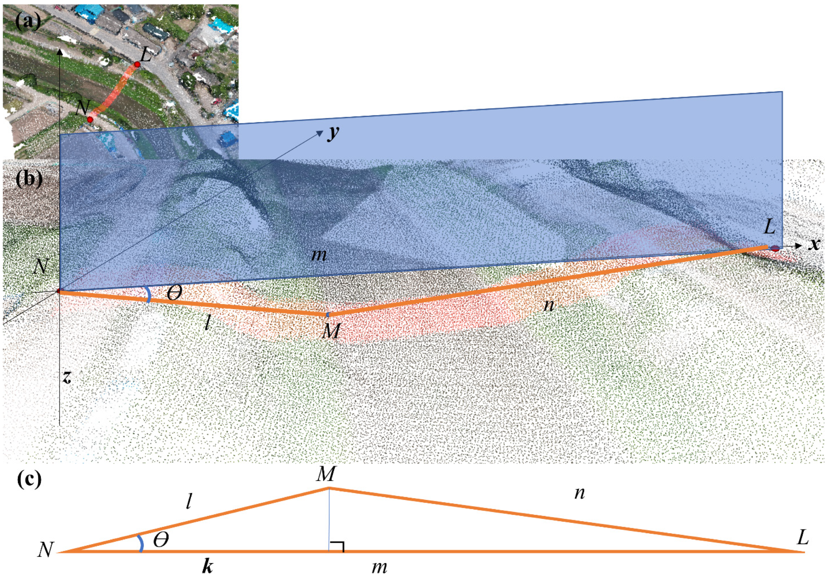
2.1. Distance Measurement of the Point Cloud

The point cloud data from UAV photography are presented with transverse mercator (TM) projection for x and y while the elevation (z-axis) was measured with respect to the WGS84 ellipsoid referring a vertical reference level. The TM projection is a conformal projection presented by Lambert in 1772. To demarcate a cross-section of a river, the point cloud data must be projected to a new coordinate system.

As an example in Figure 1, the new coordinate system can be based on the line that connects N and L points presented with the thick red line in Figure 1a. The extended thick red line is designated as the new x-coordinate, as shown in Figure 1b, and the same z-axis can be defined as the original TM data. The y-coordinate can be chosen as the axis that is perpendicular to the x–z plane and the point N is the origin of the local reference system. Let it be assumed that point M, as in Figure 1b, is selected among the selected point clouds contained in the NL line. Note that the thick red line in Figure 1a is a group of selected points from the point cloud data for defining the cross-section of the river, as shown in Figure 1b.

All of the selected red points must be aligned according to the distance from the datum point (here, N) with the new coordinate system. The new distance for the new x-coordinate can be defined as k, as shown in Figure 1c. This distance is estimated with the following equations.

The distances of l, m and n with the TM coordinate can be estimated as follows. For example, $N_{TM}\left(x\right)$ represents the x-coordinate of the TM projection for point N:

$$l=\sqrt{{\left(N_{TM}\left(x\right)-M_{TM}\left(x\right)\right)}^2+{\left(N_{TM}\left(y\right)-M_{TM}\left(y\right)\right)}^2}$$

(1)

$$m=\sqrt{{\left(N_{TM}\left(x\right)-L_{TM}\left(x\right)\right)}^2+{\left(N_{TM}\left(y\right)-L_{TM}\left(y\right)\right)}^2}$$

(2)

$$n=\sqrt{{\left(L_{TM}\left(x\right)-M_{TM}\left(x\right)\right)}^2+{\left(L_{TM}\left(y\right)-M_{TM}\left(y\right)\right)}^2}$$

(3)

From the calculated angle of MNL (Ɵ) in Equation (4), the new x-coordinate distance (k) can be calculated as in Equation (5) with the law of cosines (i.e., $n^2=l^2+m^2-2lmcos\theta$) as the following:

$$cos\theta =\frac{l^2+m^2-n^2}{2lm}$$

(4)

$$k=lcos\theta$$

(5)

In the application, there are no points that lie exactly on the NL line. Therefore, the points should be extracted in the following order.

(1) The target cross-section is to be predetermined as NL in Figure 1.

(2) Points nearby the NL line are abstracted from the point cloud dataset. Here, a width that captures the points should be determined. For example, ±1 cm above and below the NL line can be used as in the current study.

(3) The length of the collected points were estimated with Equations (1)–(5).

2.2. Procedure of the KLR

It is assumed that the current condition of the predictor x_t and its corresponding predictand y_t with the observed data (or cloud point data) pairs ($x_i$,$y_i$), for i = 1,…,n, is given for the n number of data points (i.e., the selected cloud points). In the current study, the pair ($x_i$,$y_i$) refers to the observed data of the x-coordinate (i.e., distance from the base location) and its corresponding elevation of the y-coordinate for the ith observed data (or cloud point data). The pair datapoints ($x_i$,$y_i$) were calculated as x = k in Equation (5) and y = z as the elevation of the point. This estimation process is coded in Estimate_Xdist_CrossSect_URiverX.m file with the Matlab environment. Note that the base location refers to the point that the x-coordinate of a cross-section begins. The number of neighbors (k) is also assumed to be known. The predictand Y_t is estimated (i.e., the predicted elevation with the length unit, meter in the current study) with the target x_t distance according to the following steps:

(a) Estimate the distances between the current and observed (here, point cloud data) states of the predictors for all n observations as follows:

$$D_j={\left(x_j-x_t\right)}^2\hspace{1em}\hspace{1em}j=1\dots , n$$

(6)

(b) Store the location indices for the k smallest distances.

(c) Fit the local linear regression to the observed dataset of the selected location indices [x_(p), y_(p)] for p = 1,…,k, where (p) indicates the pth decreasing ordered location index relative to the distance measure in step (a).

(c-1) Build the weight matrix using the simple selection weight as follows:

$${\mathbf{W}}_{KLR}=diag\left[\frac{1}{\delta },\frac{1/2}{\delta },...,\frac{1/k}{\delta }\right]$$

(7)

where $\delta ={\sum }_{p=1}^{k}1/p$.

$${\stackrel{⃡}{\mathbf{X}}}_t=\left(\begin{array}{c}\begin{array}{cc}1& x_t-x_{\left(1\right)}\\ 1& x_t-x_{\left(2\right)}\end{array}\\ \begin{array}{cc}1& ⋮\\ 1& x_t-x_{\left(k\right)}\end{array}\end{array}\right)$$

(8)

(c-2) Estimate the parameter vector ${\widehat{\mathit{\beta }}}_t^{KLR}$ with the weighted least square estimator from the weight matrix W_KLR in Equation (7) as

$${\widehat{\mathit{\beta }}}_t^{KLR}=({{\stackrel{⃡}{\mathbf{X}}}_t}^T{\mathit{W}}_{KLR}{\stackrel{⃡}{\mathbf{X}}}_t{)}^{-1}{{\stackrel{⃡}{\mathbf{X}}}_t}^T{\mathit{W}}_{KLR}{\mathbf{y}}_{KLR}$$

(9)

where ${\mathbf{y}}_{KLR}$ is the corresponding predicted value for the ordered observations $[y_{\left(1\right)},y_{\left(2\right)},...,y_{\left(k\right)}{]}^T$ and it is a vector with ${\widehat{\mathit{\beta }}}_t^{KLR}={\left[{\widehat{\beta }}_{0,t}^{KLR}{\widehat{\beta }}_{1,t}^{KLR}\right]}^T$.

(d) Estimate the current predictor as follows:

$$y_t={\overrightarrow{\mathbf{x}}}_t^T{\widehat{\mathit{\beta }}}_t^{KLR}$$

(10)

where ${\overrightarrow{\mathbf{x}}}_t^T=\left(1x_t\right)$.

(e) Repeat steps (a)–(d) until the required data are simulated.

The related procedure is coded in the [Predict_KLR_URiverX.m] Matlab file with the input data of the UAV point cloud dataset and its transformation with the base point of each cross-section in Equations (1)–(5).

For selecting the number of neighbors k, cross-validation (CV) based methods such as generalized cross-validation [35] are available. However, the number of data points is extremely large to apply CV-based approaches consuming a long computational time. Therefore, a heuristic approach for estimating k for the KNNR model given by $k=\sqrt{n}$ [35,36,37] was applied in the current study. The heuristic approach for KLR was tested in the current study with the multiplier as

$$k=a\sqrt{n}$$

(11)

where a is a multiplier and is a positive integer (i.e., 1, 2, 3, 4). In the result section, the appropriate multiplier was suggested for real applications.

As noted, only the partial dataset is employed for the observations rather than the whole observation dataset, unlike other regressions. For the point cloud dataset from UAV photogrammetry, this proposed approach in the current study is highly advantageous, since the neighboring data point is sufficient and the fitting of the target point must not be affected by the points that are far away from the target point. This advantage is further discussed in the Results section.

3. Simulation Study

The performance of the KLR model in fitting the point cloud data for river cross-sections is tested with the simulated point cloud data.

3.1. Model Description and Fitting

A manmade river cross-section is generally trapezoidal due to maximum discharge and easy construction [38]. Therefore, a trapezoidal channel was assumed with a 4 m top at both sides and a 6 m base width as well as a 1:1 side slope with a 6 m height, as shown by the thick solid blue line of Figure 2. The channel points were assumed to be measured with 0.1 m intervals, for a total of 161 points. It is assumed that these points work as cloud points that UAV cameras might capture in aerial surveying. The assumed cloud point dataset was generated based on the assumed 161 points (see the thick solid blue line in Figure 2), as follows:

$$Z=Y+\epsilon$$

(12)

where Y is the assumed points, and $\epsilon ~N(0,{\mathsf{\sigma }}_{\epsilon }^2)$, i.e., normally distributed error. Note that the generated data (Z) are presented with red circles in Figure 2.

In the current study, ${\sigma }_{\epsilon }^2$ = 0.2 was used following similar variability of observed data after testing several values. The magnitude of this error variance (${\sigma }_{\epsilon }^2$) represents the differences in the photo locations for the same cloud point of the real ground location (i.e., Y in this case). High variance indicates that extracted point clouds include high errors, and vice versa.

In the left and right panels of Figure 2, the simulated data are presented with red circles. The number of synthetically simulated data points was chosen to be 2 times and 10 times the assumably measured 161 points that were applied for the assumable measured trapezoid line (i.e., 322 and 1610 points), as shown in the left and right panels of Figure 2, respectively. Note that the recommended overlap is 70–80% frontal and 60% side in general cases in a photo survey [39,40] which has also been discussed by Haala, et al. [41] that it is beneficial if large redundancy is available with highly overlapping image blocks and furthermore during georeferencing, they are especially advantageous while to obtain a dense and accurate surface reconstruction. In a regular case, each cross-section point is assumed to be captured approximately 10 times. Therefore, the number of simulated data points is set to 10 times the number of trapezoidal channel points (a total of 1610), as shown in the left panels of Figure 2. Additionally, it is possible that a certain zone can be sparse with a smaller number of points. This zone is assumed to be 2 times, and 2 times the channel points were also tested, as shown in the left panels of Figure 2.

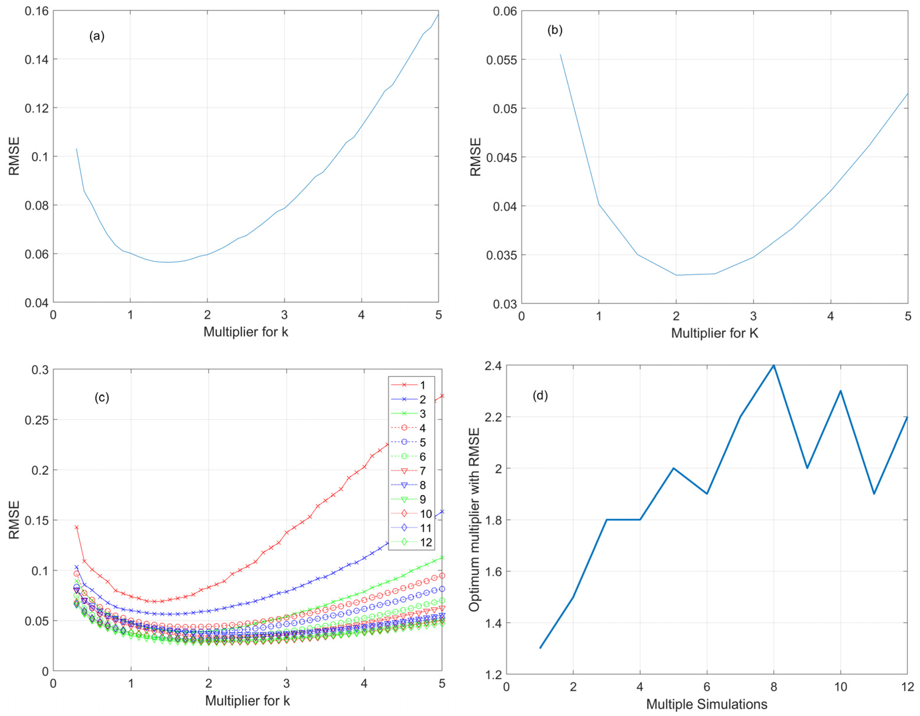
3.2. Simulation Results

In the left panels of Figure 2, the fitted cross-section line to the KLR model is shown with the dashed black line for the generated data case with two times the assumed target points, while the simulated data are presented with the red circles as noted. Note that the multiplier (a) for the number of nearest neighbors as in k = $a\sqrt{n}$ in Equation (11) was tested in this figure. As shown in the left panels of Figure 2, the multiplier a = 1, 2, 3, 4 is shown in each panel. The fitted KLR line with a smaller multiplier presents more irregularity, while the line with a higher multiplier appears to be smooth. For example, the top part of the trapezoid channel with the 22 m of the y-coordinate shows that the KLR line with the multiplier a = 1 (Figure 2(a-1)) was drawn rather coarse, but the straight shape of the original channel is preserved. At the same time, the fitted line with the high multiplier a = 4 (Figure 2(a-4)) presents a very smooth feature and presents the original top and bottom horizontal parts, which are rather too curved.

The multipliers of a = 2 and 3 in the fitted KLR model, as shown (Figure 2(a-2),(a-3)), appear to mix the smooth and horizontal features well by fitting the top and bottom horizontal lines, and the angled part of the original channel is reproduced well. This finding indicates that an appropriate multiplier (a in Equation (11)) is required to present the straight and angled trapezoid channel better.

This characteristic continues to be the case with the high number of captured cloud points, as shown in the right panels of Figure 2 (i.e., 10 times the target points, for a total of 1610 points, as shown with the red circles in this figure). It is comparable to the case of two times the target points in the left panels of Figure 2 in that all of the fitted line with the KLR model in the case of 10 times presents better the original trapezoid channel than the case of 2 times. It is obvious that a higher number of points can significantly improve the quality of the KLR model, since the nonparametric KLR model directly applies the observed data and its performance highly depends on the number of data points. In other words, while parametric models, such as linear regression and polynomial regression, estimate the parameters from the data and the parameters are employed, the nonparametric KLR model employs the data itself directly to estimate the cross-section.

The horizontal and angled trapezoid shape (i.e., the solid thick blue line in the right panels of Figure 2) is reproduced well by the KLR model (see the dashed black line), even though a coarse zig-zag line is still observed in the case of the small multiplier (i.e., a = 1, see Figure 2(b-1)). The angled portion is also too curved in the case of the high multiplier (i.e., a = 4, see Figure 2(b-4)).

The results of Figure 2 illustrate that a value between 2 and 3 can be a good selection for the multiplier. Further testing was performed to select the multiplier for the number of nearest neighbors by varying the multiplier from 0.5 to 5.0 with a 0.5 interval. The root mean square error (RMSE) and the mean absolute error (MAE) were estimated as

$$RMSE=\sqrt{\frac{1}{\mathrm{N}}{\sum }_{t=1}^N{\left(y_t-Y_t^{model}\right)}^2}$$

(13)

$$MAE=\frac{1}{\mathrm{N}}{\sum }_{t=1}^N|y_t-Y_t^{model}|$$

(14)

where $Y_t^{model}$ is the estimate from a model like the KLR in Equation (9), and $y_t$ represents the original points with N trapezoid points (here, 161 points).

The RMSE results of the KLR estimate with different multipliers (i.e., a in Equation (11)) are shown in Figure 3 for the case of 2 times (Figure 3a) the original trapezoidal points and the case of 10 times (Figure 3b). In the 2 and 10 times cases, the optimum multiplier (i.e., the smallest multiplier a) can be selected to be between 1.5 and 2.5. To fully reveal the characteristics of the multiplier with multiple simulations, all of the multiple simulations from 1 to 12, indicating the number of overlapped photos, were tested while finding the optimum multiplier. The result in Figure 3c,d shows that a smaller optimum multiplier is selected with a smaller number of overlapped photos (or multiple simulation points) as much as 1.5–2.0, and vice versa as much as 2.0–2.5.

To compare other approaches to fit the point cloud in demarcating the cross-section of a river, polynomial regression and locally weighted scatterplot smoothing (LOWESS) were also tested. The result is presented for the fitted line to the polynomial regression (top panels, Figure 4(a-1),(b-1)) and the LOWESS model (bottom panels, Figure 4(a-2),(b-2)), respectively. The fitted line to the polynomial regression of second degree (see the thick dash-dotted black line with the circle marker in the top panels of Figure 4) does not reproduce the top and bottom horizontal lines of the trapezoid channel well. Better performance in the fourth degree polynomial regression model is presented (see the dotted black line with the reverse triangle marker). However, the depth of the trapezoid center is overestimated. Other degrees of polynomial regression models were also tested, but no better performance was observed.

Furthermore, the LOWESS model was additionally fitted to the simulated trapezoid channel data. Note that the LOWESS model is also a nonparametric regression model as described already. The major difference between the LOWESS model and the KLR model is that the LOWESS model includes all of the observed data in the estimate, as shown in Equations (S2) and (S3), while the KLR model includes only the k-nearest neighbor observations, as in Equation (7). The performances of the LOWESS and KLR models were compared in detail in Lee, Ouarda and Yoon [34] for the heteroscedastic relation of time series data. The result in the study of Lee, Ouarda and Yoon [34] indicated that the KLR model reproduced an abrupt change in the heteroscedastic relation. The results of the LOWESS model are presented in the bottom panels Figure 4(a-2),(b-2)). The results indicate that the bottom part of the trapezoidal channel is reproduced well with the LOWESS model. However, the model does not reproduce the abruptly curved area well.

Additionally, different KNN models were tested and compared with the KLR model since the KLR algorithm was improved from the KNN algorithm. The result of the KNN is presented in Figure 5a and indicates that the demarcated surface from the KNN model is rather rough since the model randomly selects one among k-closest neighbors with the weight probability in Equation (7). Because no smoothing process is present in the KNN model in Figure 5a, the demarcated cross-section from this model is coarser than the one of the KLR model shown in Figure 5c. Furthermore, the KNN1 model (i.e., KNN with k = 1) selects the closest neighbor of the measured values for the channel demarcation and a coarse cross-section was made as shown in Figure 5b, similar to the one of the KNN model in Figure 5a. Note that this KNN1 model provides the result when no smoothing process is applied. The cross-section without any smoothing process will be drawn by connecting the closet points of the observed cloud point. The result of a DEM might be equivalent to the case of the KNN1 model.

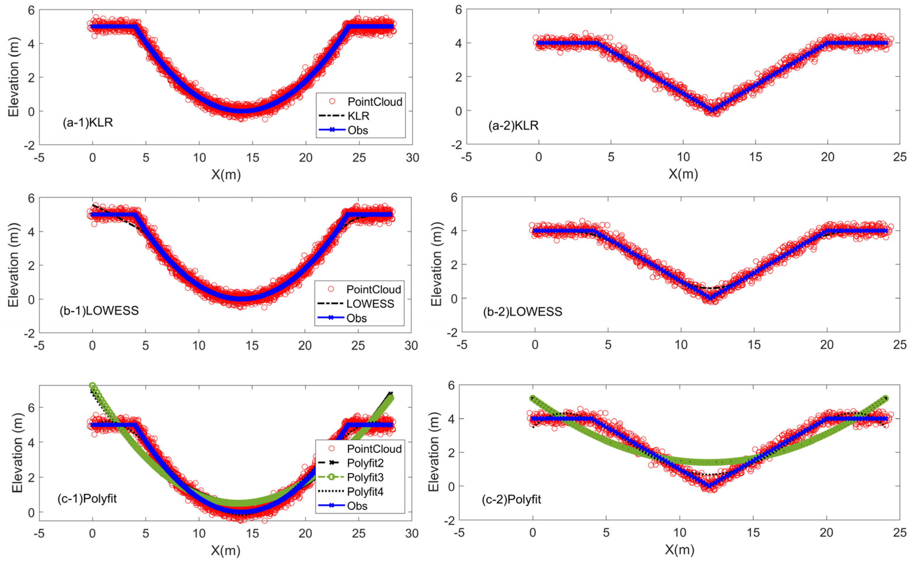
3.3. Simulation Tests with V-Shape and U-Shape Cross-Sections

In order to further test the performance of the proposed KLR model, two additional shapes of cross-sections as a U- and V-shape were tested. The U-shape channel was included, since most of natural channels present this shape and the V-shape channel can be either manmade or natural.

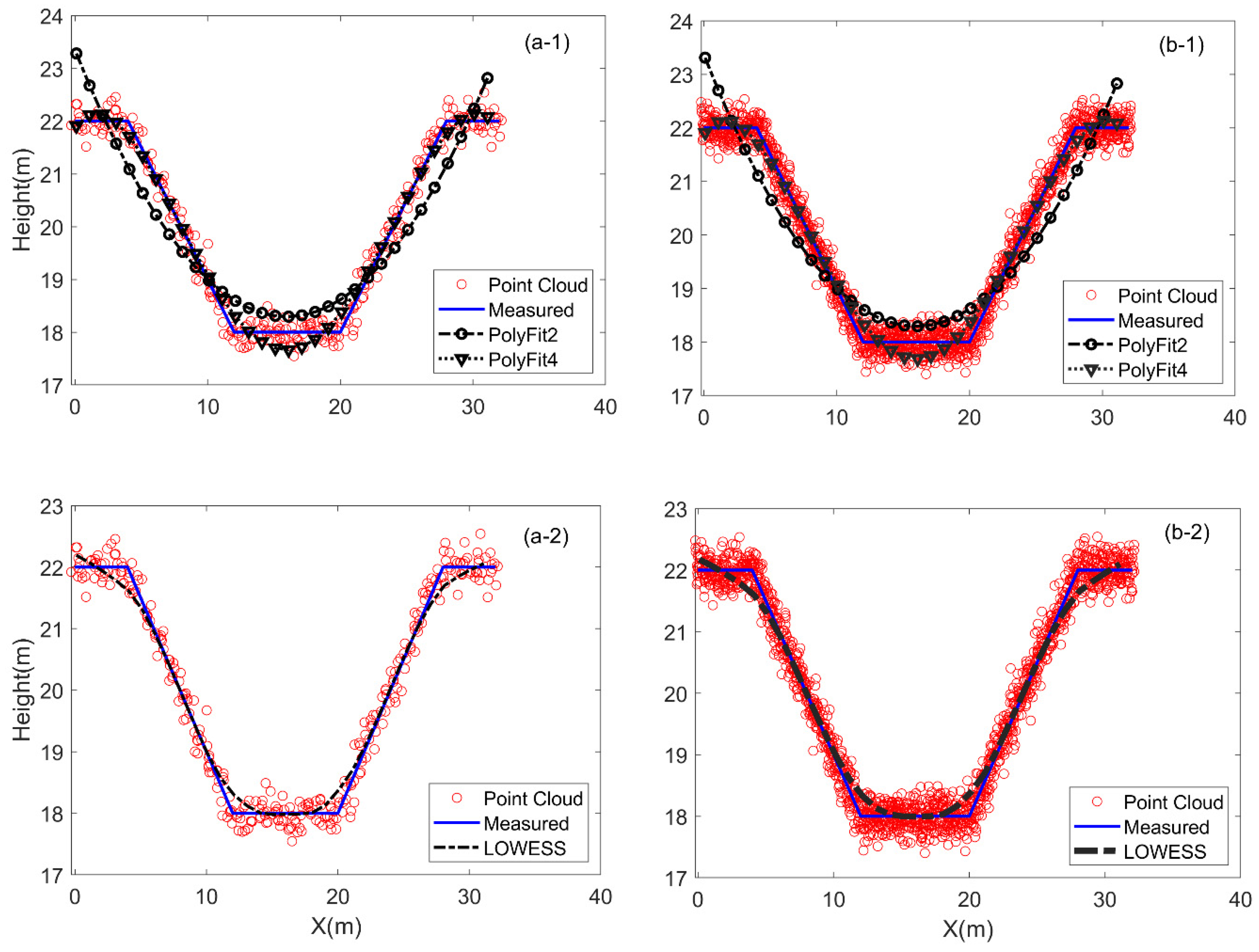
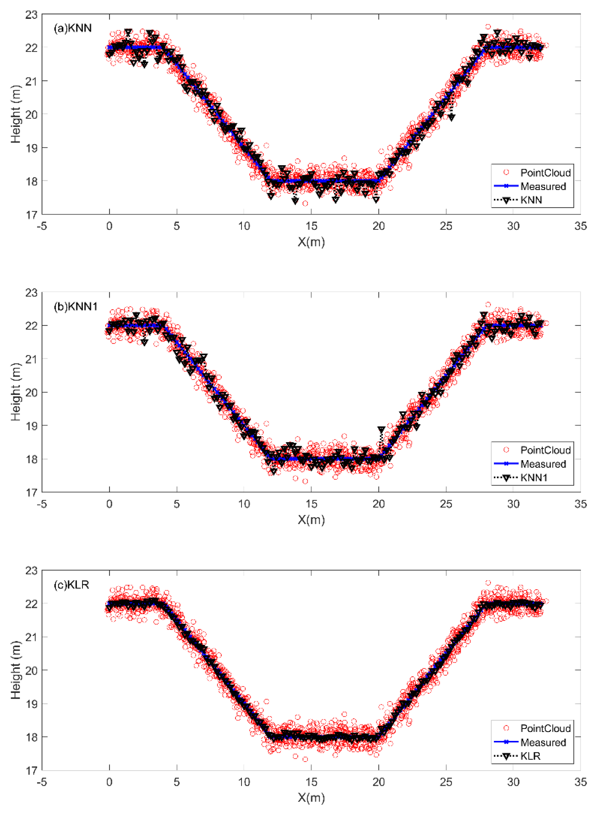
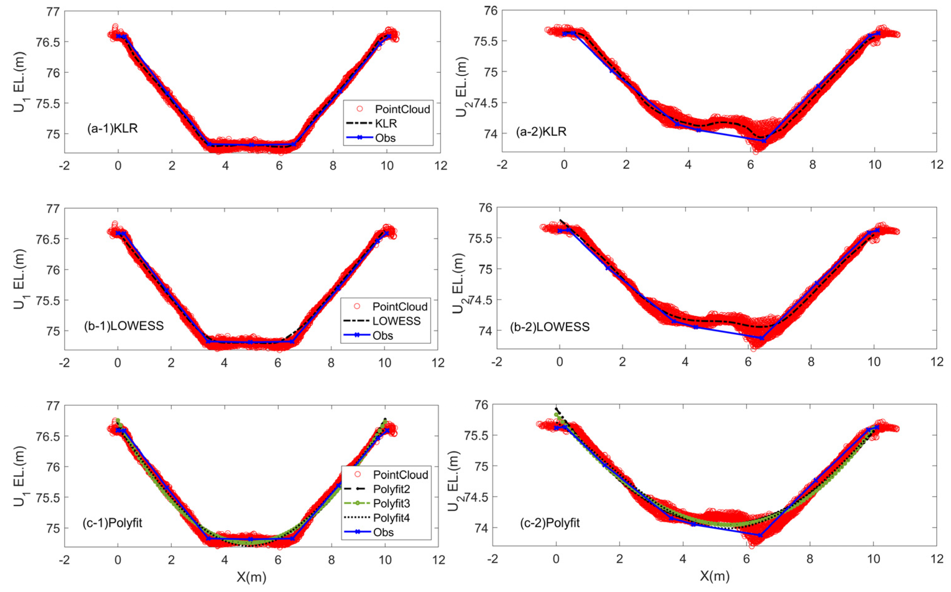
3.3.1. U-Shape Cross-Section

The U-shape cross-section that is close to a natural river was tested. The U-shape cross was modelled with a power function from Neal et al. [41] as

$$w_f=w_F{\left(\frac{h_f}{h_F}\right)}^{\frac{1}{s}}$$

(15)

$$h_f=h_F{\left(\frac{w_f}{w_F}\right)}^s$$

(16)

where $w_f$ indicates the flow width, while $w_F$ is the bank-full flow width and $h_f$ and $h_F$ are the height of flow width and the height in a bank-full condition, respectively. Additionally, s is the parameter to vary the shape of the cross-section. Here, s = 5 was set as used in Neal, Odoni, Trigg, Freer, Garcia-Pintado, Mason, Wood and Bates [41] as a basic value. To design a similar bank to the trapezoid model in the previous test, $h_F$ = 5 m and $w_F$ = 20 m was used. The number of points for the U-shape cross-section is divided to 262 points including the flat riverbank and the designed cross-section was presented in a blue solid line with cross markers as shown in the left panels of Figure 6. The synthetic point cloud data were simulated with Equation (11) and the number of point clouds was 10 times the U-shape cross-sections (i.e., 2620 points), shown with the red dots in the left panels of Figure 6.

This designed U-shape cross-section was fitted to the proposed KLR model and the other models as LOWESS and PolyFit, as shown in the left panels of Figure 6. Note that a = 2 (see Equation (11)) was applied for the KLR model from the result of the trapezoid case. The result in the left panels of Figure 6 indicates that the KLR model reproduces well the U-shape cross-section without any deviation. Meanwhile, the LOWESS model fitted the U-shape cross-section well in the middle part, but the connected part (between 4 m and 6 m of the x-coordinate) of the U-shape cross-section was not fitted well. The PolyFit model fairly fitted the U-shape cross-section with the fourth model (i.e., PolyFit4) except for slight deviation in the connected area between the slope and top bank. The PolyFit2 and PolyFit3 models poorly performed due to its limit of the flexibility.

3.3.2. V-Shape Cross-Section

One of the unique shapes of cross-sections is the V-shape for a river cross-section. The V-shape weir (or triangle shape, v-notch) was often built to provide a highly accurate solution for open channel flow measurement. The V-shape river cross-section can also be developed naturally when the sides are cut down and attacked by weathering. In addition, the loosened material slowly creeps down the slope by gravity. A V-shape cross-section was synthetically designed as shown in the right panels of Figure 6 with the height of 4 m and the top width of 16 m so that the slopes of both sides are in 1:2. The cross-section was divided to 121 points, including the flat riverbank shown with the blue solid line with cross markers in the right panels of Figure 6. Also, 10 times of the points was synthetically generated for point cloud data with Equation (11) and presented with the red dots.

The point cloud data were fitted to the KLR, LOWESS and PolyFit models and shown in Figure 6(a-2),(b-2),(c-2), respectively. Here, a = 2.0 was also employed for the KLR model. The result of the KLR model indicates that the V-shape cross-section also fitted well by the KLR model with a minimal deviation at the acute angle bottom section. Meanwhile, the LOWESS model highly deviated at the acute bottom section and slight deviation was present at the top connected part. The PolyFit model did not fairly fit the V-shape model even with PolyFit4. A further higher order model was tested (i.e., PolyFit5 and PolyFit6) and no improvement was found when increasing the order for the PolyFit model.

Table 1. Performance measures of RMSE and MAE for three different models, KLR, LOWESS and PolyFit, for synthetically simulated data of three different shape cross-sections as trapezoidal, U-shape and V-shape.

	Shape	KLR	LOWESS	PolyFit4
RMSE	Trapezoid	0.0289	0.1397	0.1565
	U-shape	0.0326	0.1868	0.1728
	V-shape	0.0325	0.1353	0.2299
MAE	Trapezoid	0.1549	0.3697	0.3789
	U-shape	0.1536	0.3158	0.3518
	V-shape	0.1558	0.2807	0.4369

presents the estimated RMSE and MAE for the three tested models of KLR, LOWESS and PolyFit4 with trapezoidal, U-shape and V-shape cross-section data. Note that only PolyFit4 was presented, since fourth degree was the best for the PolyFit models. The RMSE and MAE estimates present that the KLR model outperforms the other fitting models, while the other two models of PolyFit4 and LOWESS are comparable to each other for trapezoidal and U-shape cross-sections. For the V-shape channel, the LOWESS much better performed than the PolyFit4, since the PolyFit4 is a parametric model that connects the points rather smoothly and abrupt change cannot be modelled well due to its limited flexibility. Overall, the simulation study indicates that the proposed KLR model is a good alternative to demarcate the different shaped cross-sections.

Further, nonparametric models and other regression models, such as logistic regression [42,43,44,45], can be tested. However, the simulation study with the trapezoid channel that is similar to the real river cross-section shows that the presented KLR nonparametric model originally developed by Lee, Ouarda and Yoon [34] is suitable for demarcating the cross-section of a river. The major reason for the good performance is that the KLR model employs only k-nearest neighbor observations. This approach might not be beneficial when an overall trend is needed, and not enough observations are available. However, the point cloud data taken from UAV aerial surveying often provide a large enough number of points in the data set. Furthermore, the cross-sections in a manmade river can contain irregularity and abrupt changes by river aging. This feature can be captured only through fitting nearby observations. Therefore, the KLR model might be a suitable alternative to demarcating the cross-section of a river with the cloud point data set.

4. Experimental Study

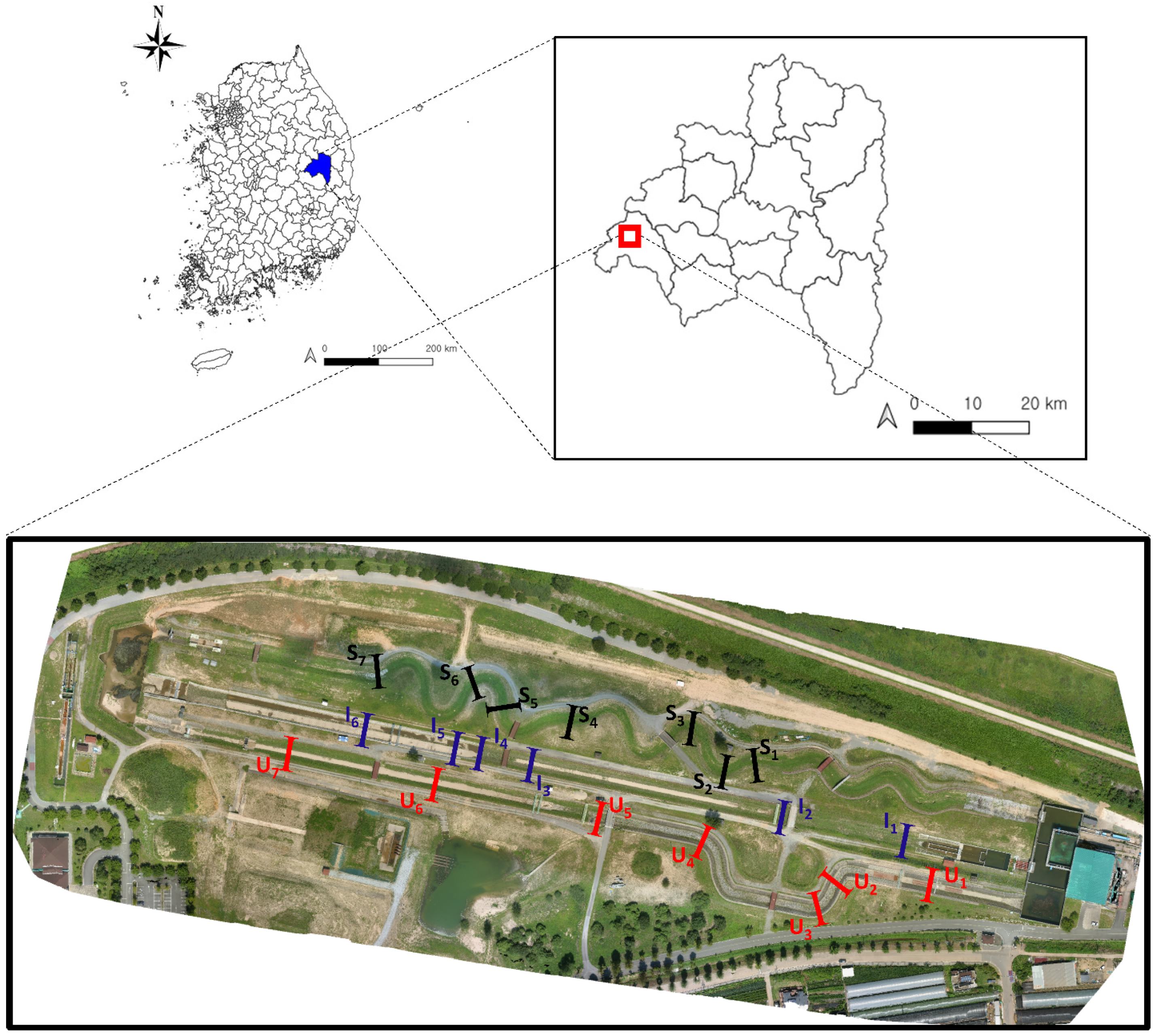
4.1. Experimental Site

In order to validate the performance of the proposed KLR model, the River Experiment Center (REC) in the Korea Institute of Civil Engineering and Building Technology was selected as an experimental site [46], as shown in Figure 7. The REC consists of a total area 193,051 m³ with three rivers of open channels with a length of 560~680 m, width of 11 m and depth of 2 m. The three channels are (1) the steep river (U-shape), (2) the meandering river (S-shape) and (3) the straight river (I-shape) as shown in the bottom panel of Figure 7. The steep river (U-shape) with a length of 590 m has a slope of 1.4% and its flow can have a velocity up to 5.0 m/s in the upstream to test the stability of bank revetment. The slope of the downstream at the steep river is 0.125% and is employed for hydraulic experiments, including vegetation development over the banks and sediment transport in the riverbed. The straight river (I-shape) with a length of 560 m has a low slope and it contains concrete compound for international cooperation study. The meandering river (S-shape) of the REC with a length of 682 m has a 1.2~1.7 sinuosity that can be employed for various experiments, including pollutant dispersion and flow structures.

On each river, six to seven cross-sections were selected, as shown in the bottom panel of Figure 7, to test the demarcation method of the current study. The channels were ground-surveyed and estimated with the UAV-based demarcation method. The steep river (S-shape) is located at the bottom and seven cross-sections were surveyed as U₁, U₂,... and U₇. The straight river (I-shape) is in the middle among three rivers with six cross-sections as I₁,.. and I₆. The meandering river (S-shape) is placed at the top and seven cross-sections were tested as S₁, S₂,... and S₇.

4.2. Application Methodology

4.2.1. Ground Surveying

For comparing demarcation methods, the real ground points were surveyed with a multiband receiver of EMLID Reach RS2 employing the global positioning system (GPS), global navigation system in Russia (GLONASS), BeiDou and Galileo. The EMLID Reach RS2 with centimeter precision was used for GNSS surveying, as shown in Figure S3a,b of the Supplementary Materials. At each channel point, about 10~15 points from the three rivers in the REC were surveyed with the GNSS system.

4.2.2. UAV Aerial Surveying

For aerial surveying of the REC, the Autel Evo II shown in Figure S3c of the Supplementary Materials was employed with 4000 × 3000 pixels with the vertical and horizontal resolutions and 2.41 cm of the average ground sampling distance. Note that the XT701 camera was applied with International Organization for Standardization(ISO)-100 and the 1/2” CMOS. The built-in flight path module of the Autel Evo II in the controller (see Figure S3d) was used to automatically obtain the aerial images of the REC, especially the targeted three experiment rivers. For the UAV photogrammetry of the REC, Pix4D Mapper was employed.

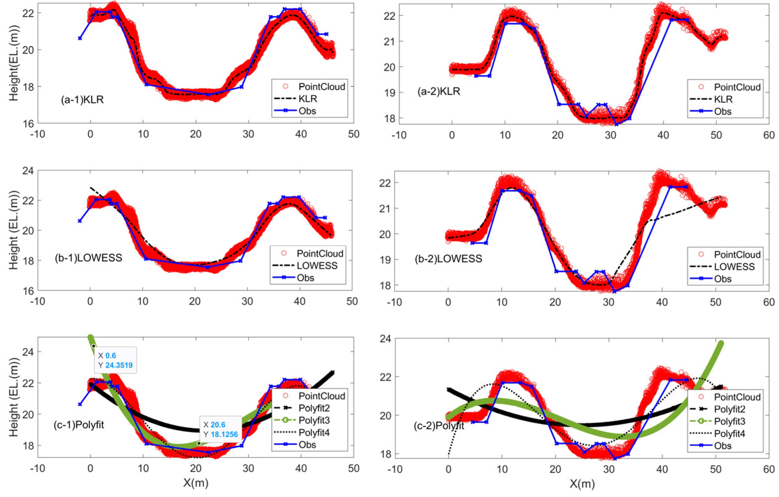
4.3. Experiment Results

In order to improve its accuracy for the UAV aerial surveying, 10 GCPs were employed with ground surveying and 34 check points were estimated for checking the entire accuracy of the REC. The RMSE of the GCPs was 0.007 m for Z and 0.017 m and 0.055 m for X and Y. The RMSE of the check points was 0.047 m for Z and 0.040 and 0.071 for X and Y. This result indicates that the UAV aerial surveying produced the ground positions of the REC, including the target three rivers and channels. The detailed quality report from the Pix4Dmapper is uploaded in the Mendeley Data repository on the website of https://data.mendeley.com/datasets/xdw4cgnvhm/2, accessed on 14 May 2024. For I₁ in the left panels of Figure 8, the point cloud (red circles) matched fairly the observed result of ground surveying (blue solid line with x marker) with a slight difference at the edge of the channel bottom in 4 m and 8 m of the x-coordinate. The KLR shown in Figure 8(a-1) draws the cross-section of I₁ following the point cloud. A similar result can be found with the LOWESS in Figure 8(b-1) except that the left-top part of the channel (i.e., around 0 m of the x-coordinate) is not preserved with the LOWESS. The polynomial regression of different degrees, shown in Figure 8(c-1), performed very similarly to each other. The method fairly depicted the cross-section of I₁ except for the left-top part of the abrupt change.

The fifth channel of the straight river (I₅) shown in the right panels of Figure 8 presents two different bottom sections. This type of channel is common in reality when a river bottom is renovated to use the portion of the river bottom as a playground or a parking place. The observed ground surveying data (blue solid line with x marker in the right panels of Figure 8) matched well the point cloud (red circles) from the UAV aerial surveying. The KLR method demarcated this channel with two bottom sections in Figure 8(a-2), including the abrupt varied part of the bottom (2 m, 5 m, 7 m and 11 m of the x-coordinate) and the top (0 m, 1 m and 12 m of the x-coordinate). The LOWESS shown in Figure 8(b-2) does not depict well the channel, especially in the abrupt changed parts. With the polynomial regression in Figure 8(c-2), a higher degree model is needed, since it includes two different bottom sections. Likely, the fourth polynomial model showed the best performance among other degree polynomials. However, the changed part was not reproduced well with any degree polynomial regression model. Similar characteristics can be observed in the other channels for I₂, I₃, I₄ and I₅ shown in Figures S4–S7 of the Supplementary Materials. The RMSE and MAE results of the tested channels are presented in

Table 2. Performance measures of RMSE for three different models as KLR, LOWESS and PolyFit for the river experiment center (REC). Note that a bold number indicates the best performance among the three models.

	No.	KLR	LOWESS	Polynomial
				2	3	4
I-shape	1	0.072	0.125	0.183	0.183	0.138
	2	0.101	0.154	0.231	0.235	0.156
	3	0.074	0.192	0.281	0.284	0.148
	4	0.054	0.12	0.17	0.174	0.177
	5	0.054	0.17	0.33	0.291	0.289
	6	0.062	0.127	0.359	0.287	0.205
U-shape	1	0.029	0.074	0.134	0.13	0.088
	2	0.066	0.118	0.182	0.155	0.119
	3	0.045	0.072	0.113	0.111	0.094
	4	0.054	0.083	0.149	0.146	0.105
	5	0.170	0.183	0.196	0.183	0.219
	6	0.131	0.183	0.374	0.363	0.201
	7	0.171	0.246	0.419	0.427	0.204
S-shape	1	0.122	0.145	0.435	0.429	0.151
	2	0.088	0.112	0.398	0.398	0.118
	3	0.204	0.216	0.428	0.416	0.203
	4	0.164	0.197	0.452	0.467	0.178
	5	0.187	0.186	0.433	0.419	0.213
	6	0.123	0.146	0.402	0.404	0.136
	7	0.145	0.146	0.48	0.488	0.22

and

Table 3. Performance measures of MAE for three different models as KLR, LOWESS and PolyFit for the river experiment center (REC). Note that a bold number indicates the best performance among the three models.

	No.	KLR	LOWESS	Polynomial
				2	3	4
I-shape	1	0.062	0.114	0.162	0.163	0.13
	2	0.083	0.135	0.194	0.197	0.125
	3	0.06	0.146	0.183	0.184	0.123
	4	0.048	0.097	0.142	0.143	0.144
	5	0.04	0.112	0.275	0.233	0.178
	6	0.05	0.098	0.299	0.224	0.139
U-shape	1	0.021	0.061	0.117	0.112	0.08
	2	0.059	0.104	0.141	0.132	0.105
	3	0.035	0.058	0.099	0.098	0.076
	4	0.039	0.072	0.126	0.126	0.091
	5	0.117	0.14	0.173	0.142	0.177
	6	0.083	0.151	0.3	0.29	0.169
	7	0.148	0.209	0.341	0.331	0.167
S-shape	1	0.094	0.113	0.377	0.339	0.12
	2	0.082	0.091	0.342	0.344	0.105
	3	0.167	0.173	0.36	0.33	0.162
	4	0.142	0.156	0.392	0.368	0.154
	5	0.147	0.136	0.379	0.374	0.19
	6	0.101	0.117	0.372	0.371	0.1
	7	0.118	0.112	0.43	0.43	0.172

. The performance measures reflected the superiority of the KLR model presenting the smallest RMSE and MAE for the channels of the straight river (i.e., I-shape).

The first channel of the steep river (i.e., U₁) is presented in the left panels of Figure 9 and it has a typical shape of a manmade river as presented in the simulation study of Section 3 in Figure 2 and Figure 4. The observed data of the ground surveying (blue solid line with x marker) matches well the aerial surveying data of the point cloud (red circles) in Figure 9. The KLR model depicted well this typical trapezoid channel, as shown in Figure 9(a-1). The LOWESS and the polynomial regression model also depicted this channel with a slight deviation at the angled bottom part (3 m and 7 m in the x-coordinate) presented in Figure 9(b-1),(c-1), respectively.

The second channel of the steep river (U₂) shown in the right panels of Figure 9 has a winding bottom. The drawn channel with the ground surveyed data shows that the varied bottom was not surveyed well. The ground surveying of the channel bottom often missed this variation due to its time limit and accessibility. In contrast, the demarcation method with the point cloud of the UAV aerial surveying depicted the detailed winding bottom. The KLR model reproduced this channel shape well, including the winding bottom as shown in Figure 9(a-2). The LOWESS also demarcated this channel fairly (see Figure 9(b-2)). However, the polynomial regression (see Figure 9(c-2)) did not depict this cross-section well by smoothing the winding bottom too much. Similar results can be observed to the other channels for U₃, U₄, U₅ and U₆ shown in Figures S4–S7 of the Supplementary Materials. The performance measures of RMSE and MAE in Table 2 and Table 3, respectively, also showed that the KLR model performed the best for the channels of the steep river with a U-shape.

The selected channels for the meandering river (S-shape) are presented in Figure 10 for S₃ (left panels) and S₆ (right panels), respectively. Both channels show the common natural U-shape in the simulation study of Section 3.3.1. The third channel of the meandering river is shown in the left panels of Figure 10 (i.e., S₃). The observed result from the ground surveying showed a slight deviation to the point cloud with the UAV aerial surveying. This deviation is also shown in other channels for the meandering river (S₁, S₂, S₄, S₅ and S₇ shown in Figures S13–S17 of the Supplementary Materials). Locating the exact cross-section might be difficult to measure especially in a meandering river and this location difficulty might result in the deviation. This U-shape channel is depicted fairly with the KLR and LOWESS models (see Figure 10(a-1),(b-1)) as well as the polynomial regression of the fourth degree (Figure 10(c-1)). The sixth channel of the meandering river (S₆) shown in the right panels of Figure 10 performed similar to the S₃ with a better representation of the observed result by the point cloud. Note that the natural U-shape channel is demarcated fairly well with all three methods shown in the simulation study. The RMSE and MAE results of the tested channels of the meandering river (S-shape) are presented in Table 2 and Table 3, respectively. The KLR model showed the smallest magnitude for S_1, S_2, S_4, S₅ and S₇. Meanwhile, the performance result for S₃ and S₆ showed that the polynomial regression with the fourth degree presented the best performance in Table 2 and Table 3. Note that some deviation between the observed result and the point cloud data is shown for the meandering river. Additionally, the S₃ and S₆ channels have the U-shape of the common natural river as discussed in the simulation study and the smooth characteristics of a U-shape channel can be reproduced well with the polynomial regression.

5. Case Study of Hapcheon

5.1. Study Area and Data Acquisition

5.1.1. Study Area

The study area is located in the Migok-cheon stream flowing through Hapcheon-gun, South Korea, as shown in Figure 11a. The Migok-cheon stream has an 8.8 km length and 13.9 km² watershed area. The slope of the stream is approximately 1/50~1/400, and the study area has a slope of 1/350. This stream conjuncts to the Hwanggang River at the end of the stream, and the Hwanggang River whose major discharge was made from Hapcheon Dam above is joined into the Nakdong River directly afterward. Therefore, the Migok-cheon stream is highly affected by the water levels of the Hwanggang River. Additionally, the fundamental engineering plan to prevent floods for the Migok-cheon stream was made in 2004 and the plan was updated in 2019 [47].

In the middle of the Hwanggang River, the Hapcheon dam is located for electricity generation and water resources. The upstream Hapcheon River consists of a number of mountains, and the slope is high, producing rapid floods and short concentration times to induce floods. For example, in August 2020, the Hapcheon dam outflowed a large amount of water downstream and induced a high-water level in the Hwanggang River. A number of streams joining the Hwanggang River overflowed due to the high level of the Hwanggang River, including the Migok-cheon stream [48]. To reduce damage from floods in the area of the Migok-cheon stream, an early warning system for floods is being considered. For the early warning system for floods, detailed cross-sections of the Migok-cheon stream must be obtained to decide which water level is appropriate for an alarm. In the current study, four sites were selected to test the performance of the proposed model located along the Migok-cheon stream as shown in Figure 11b. The Naesamhak village is located on the left side of the river, while only cultivation land is on the right side indicating that the left bank has higher importance to water managers. The Unsam bridge is also placed in the middle the Migok-cheon stream.

5.1.2. Data Acquisition

Aerial photos over the selected Migok-cheon were obtained with the unmanned aerial vehicle (also termed drone), DJI Phantom 4. This UAV is one of the most popular professional drones on the market and contains an advanced stereo vision positioning system that provides precise hovering even without satellite positioning support [49]. The camera applied is FC3411 with ISO-110 and the image sensor of 1/2.3” CMOS, and the images taken from DJI Phantom 4 are 5472 × 3648 pixels at approximately 10 M with the horizontal and vertical resolutions of 75 DPI. Pix4Dcapture was employed to map the target area. The flight with a height of 75 meters was made on 8 July 2021.

Ground control points (GCPs) are the points on the ground that have measured or known coordinates. To obtain GCPs, 10 specific points were measured over the target area on the ground with global positioning system (GPS) surveying. The EMLID Reach RS2 (https://emlid.com/reachrs2/, accessed on 1 May 2024), multiband RTK GNSS receiver, with centimeter precision, was employed for GNSS surveying.

The aerial photos were postprocessed to build a point cloud dataset with WebODM. The WebODM (https://github.com/OpenDroneMap/WebODM, accessed on 1 May 2024) is an open-source tool for generating map point clouds, and terrain and 3D surface models from aerial images.

5.2. Results

5.2.1. Selected Sites for Cross-Section Demarcation

The four tested sites in the Migok-cheon stream are presented in Figure 11b. The overall produced point cloud dataset for the UAV surveying area is presented in the top-left panel of Figure 11b, and the picture of the top-left panel consists of only the collected points. Site-1 is located in the middle of the study area, while Site-2 is in the upper part of the area. Since the nearby area of Site-1 is located in the middle of the UAV surveying coverage, several images can be overleaped and captured for the same points. The other two sites (Site-3 and Site-4) that are located between Site-1 and Site-2 were added for further comparison.

Therefore, the number of points for demarcating a cross-section of the river might be sufficient to capture the detailed characteristics of the cross-section (see the top-right panel of Figure 11b) like in Site-1 (see the red dots in the left panels of Figure 12) as well as Site-3 and Site-4 (see Figure 13). In contrast, Site-2 is located at the upper part of the coverage area, which indicates that the number of points to capture a target cross-section is also limited as shown in the red dots in the right panels of Figure 12. Furthermore, part of the cross-sectional area can be missing due to technical and environmental limitations, such as waterbodies and riverbank sides as well as shadow from the sun. For example, there are some areas in which no cloud point data exists, as on the right side of Site-2. This point is intentionally selected to verify the model performance in such a case.

5.2.2. Demarcation of Selected Cross-Sections

The demarcated cross-sections for the selected sites (i.e., Site-1, Site-2, Site-3 and Site-4) are illustrated in Figure 12 and Figure 13, respectively. Additionally, the RMSE and MAE estimates are presented in

Table 4. Performance measures of RMSE and MAE for three different models as KLR, LOWESS and PolyFit for four sites of Hapcheon-gun.

	Site No.	KLR	LOWESS	PolyFit2	PolyFit3	PolyFit4
RMSE	Site-1	0.4063	0.8389	1.8548	1.8046	1.4218
	Site-2	0.4010	0.6736	1.3762	1.1252	0.8753
	Site-3	0.3236	0.4514	1.4722	1.4327	0.9753
	Site-4	0.4786	0.9419	1.3834	1.9593	0.7068
MAE	Site-1	0.5393	0.8197	1.3034	1.2934	1.1224
	Site-2	0.4406	0.5764	1.1758	1.1611	0.9482
	Site-3	0.5746	0.7439	1.1536	1.0342	0.8221
	Site-4	0.6422	0.8307	1.1500	1.1057	0.7615

to show the performance of the presented models. In the left panels of Figure 12, the extracted cloud points for Site-1 are presented with red circles. As noted, a number of cloud points were extracted from the UAV aerial photogrammetry for Site-1, since the site is located with enough photo coverage. The KLR fitted line shown with the dashed black line of Figure 12(a-1) indicates that the fitted line reproduces the characteristics of the natural cross-section of the river well, including the overall trapezoidal shape and the natural bumps at the bottom. This line is compared with field measurements reported in BRTMA [47]. Slight differences can be seen between field measurements (shown with the solid blue line with the x marker) and the KLR fitted line since field measurements took place approximately 3 years ago. The LOWESS model and the PolyFit models with the degree of 2, 3 and 4 were also tested and their results were presented in Figure 12(b-1),(c-1), respectively. The LOWESS fairly fitted the point cloud data except the left side between 14 m and 20 m of the x-coordinate with deviation from major cloud points. Meanwhile, all the Polyfit models (i.e., second, third and fourth degrees) did not fit the point cloud data fairly with high deviation from the point cloud.

The cross-section of Site-2 is presented in the right panels of Figure 12 and shows that the middle part of the left slope of the stream has no cloud point data. The KLR fitted line shows that the overall characteristics of the cross-section are reproduced. Even the missing part of the cross-section between 12 m and 17 m of the x-coordinate is also interpolated well with the KLR model by comparing field measurements (see the solid blue line with the x marker in the right panels of Figure 12). Some differences between the fitted line and the field measurement might result from the year difference. This result indicates that a missing part of the aerial surveying can be filled up with the interpolation of the KLR method. This can be a good benefit of the KLR model in demarcating the cross-sections with the UAV point cloud data, since this missing data can be sometimes inevitable. Otherwise, further UAV surveying might be required to fill up the gap costing additional time and money.

The LOWESS model also fitted the point cloud data fairly well through all the section (see Figure 12(b-2)) except that slight deviation can be observed on the right side of the top bank between 40 m and 42 m of the x-coordinate. Further, the missing part (between 12 m and 17 m of the x-coordinate) was not fairly interpolated with the LOWESS model. This might be induced from the lack of the points in this missing area, since the farther left side has denser points and the predicted points from the LOWESS model might be affected by these dense points. The PolyFit does not estimate the model well due to the lack of model flexibility to an abrupt change of the cross-sections as mentioned.

Site-3 contains a number of cloud points as shown in the left panels of Figure 13. The KLR model fitted the cloud points well while the LOWESS model presents a good performance (see Figure 13(b-1)), but the deviation from the cloud points is observed in the left bank section (i.e., between 0 m and 3 m of x-coordinate). The PolyFit4 model as shown (in Figure 13(c-1)) fairly performs in fitting the cloud data points. It is because the shape of the cross-section is rather smoothly curved. The Site-4 result shown in the right panels of Figure 13 indicates that the KLR model (Figure 13(a-2)) performs well in fitting the cloud points from the UAV surveying, while the LOWESS model (Figure 13(b-2)) presents significant deviation from the cloud points on the right side and the PolyFit models (Figure 13(c-2)) did not fairly perform.

The performance measures of RMSE and MAE are presented in Table 4 for all four sites and three tested models. The RMSE value of KLR is between 0.32 and 0.47 while that of the LOWESS and PolyFit is between 0.45 and 0.94 and 0.71 and 1.4. This performance result indicates that KLR outperforms the LOWESS and PolyFit models for all four sites. The PolyFit model (RMSE: 0.70 and MAE: 0.76) better performs than the LOWESS model (RMSE: 0.94 and MAE: 0.83) for Site-4, while LOWESS is always better for other sites. The overall result of the case study indicates that the KLR method can reproduce the characteristics of the cross-section of a natural river and be a good alternative to demarcate a cross-section in a river.

6. Discussion

The results of the synthetic simulation study and two case studies as well as the experiment study of the REC site present that the proposed KLR model can demarcate the cross-sections of a river with different shapes. However, there are some limitations and conditions to apply the proposed model in the demarcation of river cross-sections. At first, UAV sensors cannot penetrate water depth unless bathymetric technology is not applied. Currently, river photogrammetry with bathymetry data have been applied to penetrate water bodies using specialized sensors, such as Light Detection and Ranging (LiDAR), which is called bathymetry LiDAR [50,51]. The case study of the current study does not use bathymetry data, since the water depth is very shallow and not critical to illustrate a river cross-section. The proposed KLR model with the point cloud data must be carefully applied to a dry stream or very shallow river with the water surface whose level is ignorable especially for its discharge amount. Otherwise, bathymetry data must be applied using a special sensor (e.g., bathymetry LiDAR).

Secondly, the KLR model should define the number of K-neighbors. The result of the tested model illustrates that the value of 1.5–2.5 for ‘a’ in Equation (11) might be a good range. Further estimation procedures might be required in some cases to produce cross-sections that are more accurate. However, the value is not very sensitive at each case presented in the current study. Note that a = 2.0 was employed for the U-shape and V-shape synthetic cross-section and the case study without any further estimation procedure.

Furthermore, traditional ground surveying might be essential to supplement UAV or LiDAR-based point clouds for the purpose of hydraulic modeling due to the penetration capability of sensors and sensitivity even with capable sensors. A ground surveying for a few cross-sections can be performed in addition to UAV surveying. The ground-surveyed cross-sections can be employed to validate the UAV-based cross-sections. This additional ground surveying might greatly improve the quality of the UAV-based cross-sections.

The UAV-based demarcation of cross-sections still has some limitations and conditions to ensure its credibility, such as water penetration and additional requirement of ground surveying. Nevertheless, the proposed KLR model can be applicable to the demarcation of different cross-section shapes with UAV point cloud data. In addition, UAV sensors and photogrammetry technology have been developed so that the current KLR method might be more useful and applicable with UAV-based data. UAV surveying can be a potential surrogate for its relatively cheap and time-saving. The river cross-section with UAV surveying can be beneficial when the ground surveying cannot be made. After initial ground surveying, further resources may not be available for additional ground surveying. In this case, the river cross-section with UAV surveying can extract any place inside the surveyed area.

7. Summary and Conclusions

The current study presents a nonparametric fitting method, KLR, to the point cloud data from UAV areal surveying to demarcate the cross-section of a river. Other than general fitting data, the cross-section of a natural river generally contains sudden variation, an angled shape and even bumps as well as a linear shape. To accommodate all of those features of natural and manmade cross-sections, a highly flexible fitting model is requested. Furthermore, the observed data point from UAV surveying is large enough for the point cloud dataset. Therefore, the KLR model can be chosen to fit the point cloud data for cross-sections. Different river shapes with the simulation study and the experimental site study of the REC were made as well as two case studies of the Migok-cheon stream, Hapcheon-gun and the Pori-cheon stream, Yecheon-gun. From the extensive applications of the proposed model in the current study, the results conclude that the suggested KLR model can reproduce the critical characteristics of the different shape cross-sections of a river with the point cloud data from UAV aerial surveying.

The major limitation of the point cloud data employed in the current study is that RGB photographs were employed and the vegetation inside the river could generate an obscure cross-sectional shape. Further optical instruments, such as hyperspectral and lidar sensors, could be tested to overcome this limitation. However, a perfect solution that can remove the vegetation inside rivers has not yet been developed. To avoid this issue, points of the cross-section where little vegetation exists can be selected. Further, a general UAV sensor cannot penetrate a water body and a special sensor (e.g., bathymetry LiDAR and multispectral camera) must be employed to capture the shape of the cross-section below the water surface and in a developing stage [52,53]. Therefore, special care must be taken to apply the current model to UAV surveying data. The current demarcation method for a cross-section must be applied to a dry stream or very shallow stream whose flow does not affect the discharge amount. Otherwise, bathymetry data must be employed for demarcating a cross-section of a river. Since the sensors that can penetrate water body and UAV technologies are developing fast, the proposed KLR model with the UAV surveying might become more suitable in the near future to demarcate a cross-section. Seasonal rivers with canopy covers also cannot be measured well with aerial photogrammetry. Further technical development such as a LiDAR survey can overcome this limitation.

The proposed KLR method can be easily adopted for other demarcation cases, such as buildings and structures. The proposed KLR method is a rather simple and direct approach for demarcating an area and structures. Additionally, other nonparametric techniques, such as LOWESS, can be further tested with extensive testing and adjustment. The current study focused on the KLR model, since the clustered data setting is obvious and easy to apply.

References

1. Watanabe, Y.; Kawahara, Y. UAV Photogrammetry for Monitoring Changes in River Topography and Vegetation. Procedia Eng. 2016, 154, 317–325. [Google Scholar] [CrossRef]
2. Hugenholtz, C.H.; Whitehead, K.; Brown, O.W.; Barchyn, T.E.; Moorman, B.J.; LeClair, A.; Riddell, K.; Hamilton, T. Geomorphological mapping with a small unmanned aircraft system (sUAS): Feature detection and accuracy assessment of a photogrammetrically-derived digital terrain model. Geomorphology 2013, 194, 16–24. [Google Scholar] [CrossRef]
3. Remondino, F.; Barazzetti, L.; Nex, F.; Scaioni, M.; Sarazzi, D. UAV photogrammetry for mapping and 3d modelingCurrent status and future perspectives. In Proceedings of the International Archives of the Photogrammetry, Remote Sensing and Spatial Information Sciences—ISPRS Archives, Zurich, Switzerland, 14–16 September 2011; pp. 25–31. [Google Scholar]
4. Siebert, S.; Teizer, J. Mobile 3D mapping for surveying earthwork projects using an Unmanned Aerial Vehicle (UAV) system. Autom. Constr. 2014, 41, 1–14. [Google Scholar] [CrossRef]
5. Lin, C.; Chen, S.Y.; Chen, C.C.; Tai, C.H. Detecting newly grown tree leaves from unmanned-aerial-vehicle images using hyperspectral target detection techniques. ISPRS J. Photogramm. Remote Sens. 2018, 142, 174–189. [Google Scholar] [CrossRef]
6. Marfai, M.A.; Sunarto; Khakim, N.; Fatchurohman, H.; Cahyadi, A.; Wibowo, Y.A.; Rosaji, F.S.C. Tsunami hazard mapping and loss estimation using geographic information system in Drini Beach, Gunungkidul Coastal Area, Yogyakarta, Indonesia. Proc. E3S Web Conf. 2019, 76, 03010. [Google Scholar] [CrossRef]
7. Srivastava, K.; Pandey, P.C.; Sharma, J.K. An approach for route optimization in applications of precision agriculture using uavs. Drones 2020, 4, 58. [Google Scholar] [CrossRef]
8. Taddia, Y.; Pellegrinelli, A.; Corbau, C.; Franchi, G.; Staver, L.W.; Stevenson, J.C.; Nardin, W. High-resolution monitoring of tidal systems using UAV: A case study on poplar island, MD (USA). Remote Sens. 2021, 13, 1364. [Google Scholar] [CrossRef]
9. Wang, S.; Ahmed, Z.; Hashmi, M.Z.; Pengyu, W. Cliff face rock slope stability analysis based on unmanned arial vehicle (UAV) photogrammetry. Geomech. Geophys. Geo-Energy Geo-Resour. 2019, 5, 333–344. [Google Scholar] [CrossRef]
10. Yan, Y.; Ma, S.; Yin, S.; Hu, S.; Long, Y.; Xie, C.; Jiang, H. Detection and Numerical Simulation of Potential Hazard in Oil Pipeline Areas Based on UAV Surveys. Front. Earth Sci. 2021, 9, 665478. [Google Scholar] [CrossRef]
11. Gracchi, T.; Rossi, G.; Stefanelli, C.T.; Tanteri, L.; Pozzani, R.; Moretti, S. Tracking the evolution of riverbed morphology on the basis of uav photogrammetry. Remote Sens. 2021, 13, 829. [Google Scholar] [CrossRef]
12. Langhammer, J. UAV monitoring of stream restorations. Hydrology 2019, 6, 29. [Google Scholar] [CrossRef]
13. Lee, G.; Choi, M.; Yu, W.; Jung, K. Creation of river terrain data using region growing method based on point cloud data from UAV photography. Quat. Int. 2019, 519, 255–262. [Google Scholar] [CrossRef]
14. Sanhueza, D.; Picco, L.; Ruiz-Villanueva, V.; Iroumé, A.; Ulloa, H.; Barrientos, G. Quantification of fluvial wood using UAVs and structure from motion. Geomorphology 2019, 345, 106837. [Google Scholar] [CrossRef]
15. Tomsett, C.; Leyland, J. Remote sensing of river corridors: A review of current trends and future directions. River Res. Appl. 2019, 35, 779–803. [Google Scholar] [CrossRef]
16. Anders, N.; Smith, M.; Suomalainen, J.; Cammeraat, E.; Valente, J.; Keesstra, S. Impact of flight altitude and cover orientation on Digital Surface Model (DSM) accuracy for flood damage assessment in Murcia (Spain) using a fixed-wing UAV. Earth Sci. Inform. 2020, 13, 391–404. [Google Scholar] [CrossRef]
17. Andreadakis, E.; Diakakis, M.; Vassilakis, E.; Deligiannakis, G.; Antoniadis, A.; Andriopoulos, P.; Spyrou, N.I.; Nikolopoulos, E.I. Unmanned aerial systems-aided post-flood peak discharge estimation in ephemeral streams. Remote Sens. 2020, 12, 4183. [Google Scholar] [CrossRef]
18. Zakaria, S.; Mahadi, M.R.; Abdullah, A.F.; Abdan, K. Aerial platform reliability for flood monitoring under various weather conditions: A review. In Proceedings of the International Archives of the Photogrammetry, Remote Sensing and Spatial Information Sciences—ISPRS Archives; Springer: Cham, Switzerland, 2018; pp. 591–602. [Google Scholar]
19. Izumida, A.; Uchiyama, S.; Sugai, T. Application of UAV-SfM photogrammetry and aerial lidar to a disastrous flood: Repeated topographic measurement of a newly formed crevasse splay of the Kinu River, central Japan. Nat. Hazards Earth Syst. Sci. 2017, 17, 1505–1519. [Google Scholar] [CrossRef]
20. Kaewwilai, A.J. Analysis of Flood Patterns in Adams County, Pennsylvania Utilizing Drone Technology and Computer Simulations Analysis of Flood Patterns in Adams County. Pa. Util. Drone 2019, 57, 1–20. [Google Scholar]
21. Perks, M.T.; Russell, A.J.; Large, A.R.G. Technical note: Advances in flash flood monitoring using unmanned aerial vehicles (UAVs). Hydrol. Earth Syst. Sci. 2016, 20, 4005–4015. [Google Scholar] [CrossRef]
22. Tsunetaka, H.; Hotta, N.; Hayakawa, Y.S.; Imaizumi, F. Spatial accuracy assessment of unmanned aerial vehicle-based structures from motion multi-view stereo photogrammetry for geomorphic observations in initiation zones of debris flows, Ohya landslide, Japan. Prog. Earth Planet. Sci. 2020, 7, 24. [Google Scholar] [CrossRef]
23. Carbonneau, P.E.; Dietrich, J.T. Cost-effective non-metric photogrammetry from consumer-grade sUAS: Implications for direct georeferencing of structure from motion photogrammetry. Earth Surf. Process. Landf. 2017, 42, 473–486. [Google Scholar] [CrossRef]
24. Lee, T.; Singh, V.P.S.; Ha, T.H. UAV Photogrammetry-based Flood Early Warning System applied to Migok-cheon Stream, South Korea. J. Hydrol. Eng. 2022. in review. [Google Scholar] [CrossRef]
25. Gichamo, T.Z.; Popescu, I.; Jonoski, A.; Solomatine, D. River cross-section extraction from the ASTER global DEM for flood modeling. Environ. Model. Softw. 2012, 31, 37–46. [Google Scholar] [CrossRef]
26. Petikas, I.; Keramaris, E.; Kanakoudis, V. Calculation of multiple critical depths in open channels using an adaptive cubic polynomials algorithm. Water 2020, 12, 799. [Google Scholar] [CrossRef]
27. Pilotti, M. Extraction of cross sections from digital elevation model for one-dimensional dam-break wave propagation in mountain valleys. Water Resour. Res. 2016, 52, 52–68. [Google Scholar] [CrossRef]
28. Petikas, I.; Keramaris, E.; Kanakoudis, V. A novel method for the automatic extraction of quality non-planar river cross-sections from digital elevation models. Water 2020, 12, 3553. [Google Scholar] [CrossRef]
29. Sanders, B.F. Evaluation of on-line DEMs for flood inundation modeling. Adv. Water Resour. 2007, 30, 1831–1843. [Google Scholar] [CrossRef]
30. Tarekegn, T.H.; Haile, A.T.; Rientjes, T.; Reggiani, P.; Alkema, D. Assessment of an ASTER-generated DEM for 2D hydrodynamic flood modeling. Int. J. Appl. Earth Obs. Geoinf. 2010, 12, 457–465. [Google Scholar] [CrossRef]
31. Matgen, P.; Hostache, R.; Schumann, G.; Pfister, L.; Hoffmann, L.; Savenije, H.H.G. Towards an automated SAR-based flood monitoring system: Lessons learned from two case studies. Phys. Chem. Earth 2011, 36, 241–252. [Google Scholar] [CrossRef]
32. Azizian, A.; Brocca, L. Determining the best remotely sensed DEM for flood inundation mapping in data sparse regions. Int. J. Remote Sens. 2020, 41, 1884–1906. [Google Scholar] [CrossRef]
33. Biswal, S.; Sahoo, B.; Jha, M.K.; Bhuyan, M.K. A hybrid machine learning-based multi-DEM ensemble model of river cross-section extraction: Implications on streamflow routing. J. Hydrol. 2023, 625, 129951. [Google Scholar] [CrossRef]
34. Lee, T.; Ouarda, T.B.M.J.; Yoon, S. KNN-based local linear regression for the analysis and simulation of low flow extremes under climatic influence. Clim. Dyn. 2017, 49, 3493–3511. [Google Scholar] [CrossRef]
35. Lall, U.; Sharma, A. A nearest neighbor bootstrap for resampling hydrologic time series. Water Resour. Res. 1996, 32, 679–693. [Google Scholar] [CrossRef]
36. Lee, T.; Ouarda, T.B.M.J. Identification of model order and number of neighbors for k-nearest neighbor resampling. J. Hydrol. 2011, 404, 136–145. [Google Scholar] [CrossRef]
37. Lee, T.; Salas, J.D.; Prairie, J. An Enhanced Nonparametric Streamflow Disaggregation Model with Genetic Algorithm. Water Resour. Res. 2010, 46, W08545. [Google Scholar] [CrossRef]
38. Chow, V.T. Open Channel Hydraulics; McGraw-Hill: New York, NY, USA, 1959; p. 350. [Google Scholar]
39. Falkner, E.; Morgan, D. Aerial Mapping: Methods and Applications; CRC Press: Boca Raton, FL, USA, 2001; p. 216. [Google Scholar]
40. Weilberg, M. Photogrammetry and Remote Sensing; Syrawood Publishing House: New York, NY, USA, 2016; p. 216. [Google Scholar]
41. Neal, J.C.; Odoni, N.A.; Trigg, M.A.; Freer, J.E.; Garcia-Pintado, J.; Mason, D.C.; Wood, M.; Bates, P.D. Efficient incorporation of channel cross-section geometry uncertainty into regional and global scale flood inundation models. J. Hydrol. 2015, 529, 169–183. [Google Scholar] [CrossRef]
42. Ahmad, M.I.; Sinclair, C.D.; Werritty, A. Log-logistic flood frequency analysis. J. Hydrol. 1988, 98, 205–224. [Google Scholar] [CrossRef]
43. Elek, P.; Márkus, L. A long range dependent model with nonlinear innovations for simulating daily river flows. Nat. Hazards Earth Syst. Sci. 2004, 4, 277–283. [Google Scholar] [CrossRef]
44. Orlowsky, B.; Bothe, O.; Fraedrich, K.; Gerstengarbe, F.W.; Zhu, X. Future climates from bias-bootstrapped weather analogs: An application to the Yangtze River basin. J. Clim. 2010, 23, 3509–3524. [Google Scholar] [CrossRef]
45. Simonoff, J.S. Smoothing Methods in Statistics; Springer: New York, NY, USA, 1996; p. 353. [Google Scholar]
46. Lee, C.; Kim, J.; Kang, W.; Ji, W.; Jung, S. KICT River Experiment Center. Water Future 2022, 55, 91–97. [Google Scholar]
47. BRTMA. Reports of Fundamental River Plan for Hwanggang Downstream Rivers. 2019; Volume 1021. Available online: http://www.river.go.kr/ (accessed on 14 May 2024).
48. Seong, K.; Lee, S.O.; Jung, H.J.; Lee, T. Safety first? Lessons from the Hapcheon Dam flood in 2020. Nat. Hazards 2020. in review. [Google Scholar]
49. Hamdi, D.A.; Iqbal, F.; Alam, S.; Kazim, A.; MacDermott, A. Drone forensics: A case study on DJI phantom 4. In Proceedings of the Proceedings of IEEE/ACS International Conference on Computer Systems and Applications, AICCSA, Abu Dhabi, United Arab Emirates, 3–7 November 2019. [Google Scholar]
50. Fernandez-Diaz, J.C.; Glennie, C.L.; Carter, W.E.; Shrestha, R.L.; Sartori, M.P.; Singhania, A.; Legleiter, C.J.; Overstreet, B.T. Early results of simultaneous terrain and shallow water bathymetry mapping using a single-wavelength airborne LiDAR sensor. IEEE J. Sel. Top. Appl. Earth Obs. Remote Sens. 2014, 7, 623–635. [Google Scholar] [CrossRef]
51. Allouis, T.; Bailly, J.; Pastol, Y.; Le Roux, C. Comparison of LiDAR waveform processing methods for very shallow water bathymetry using Raman, near-infrared and green signals. Earth Surf. Process. Landf. 2010, 35, 640–650. [Google Scholar] [CrossRef]
52. Lee, C.H.; Liu, L.W.; Wang, Y.M.; Leu, J.M.; Chen, C.L. Drone-Based Bathymetry Modeling for Mountainous Shallow Rivers in Taiwan Using Machine Learning. Remote Sens. 2022, 14, 3343. [Google Scholar] [CrossRef]
53. Mandlburger, G.; Kölle, M.; Nübel, H.; Soergel, U. BathyNet: A Deep Neural Network for Water Depth Mapping from Multispectral Aerial Images. PFG—J. Photogramm. Remote Sens. Geoinf. Sci. 2021, 89, 71–89. [Google Scholar] [CrossRef]
Figure 1. Example of the distance measurement: (a) aerial photo with a selected cross-section (two red dots, L and N and thick red line); (b) magnified photo of the panel (a) with assisted 3D axis (x, y and z) and the selected point (M); (c) emphasized triangle with the points of NML. Note that (1) the cross-section can be defined with the x-axis by connecting points N and L with the line; (2) point M is the example point that contains the red line at the panel (a), which is a group of points in reality; and (3) the actual distance of M from N in the x-axis is represented as k, which can be designated as N to the point that meets line NL perpendicularly from M. The aerial images were taken from the authors.
Remotesensing 16 01820 g001
Figure 2. Assumed synthetic trapezoidal channel (not a real one) to test the KLR model (thick black dotted line) for the simulated point cloud data with Equation (S6) to a total of 322 points (red dots) with different portions of the number of neighbors ( k = a n , here a = 1, 2, 3 and 4 at each row panels). Note that (1) the trapezoidal sections are consistent with a 4 m top both sides and a 6 m base width as well as a 1:1 side slope with a 6 m height; (2) the number of points for the channel was divided at each 0.1 m to a total of 161 points (blue line); (3) two times the divided data are simulated with Equation (S6) to a total of 322 points (red dots) shown in the left panels (a) while five times larger point data than the points in the left panels (a) were simulated and shown in the right panels (b); and (4) the elevation of the bottom channel was assumed to be 18 m.
Remotesensing 16 01820 g002
Figure 3. Root mean square error (RMSE) between the KLR estimate with different multipliers (a) of the number of neighbors ( k = a n ) and the original trapezoid points for the case of 2 times the original points (a) and 10 times (b); with the original trapezoid points for all of the cases between 1 and 12 times the original points (c); as well as the optimum multiplier (d) with the RMSE value at the top panel for each multiple simulation. Note that increasing the number of multiple simulations indicates that the number of overlapped photos increases and the cloud points are multiplied.
Remotesensing 16 01820 g003
Figure 4. Polynomial regression (top panels, (a-1,b-1)) with the black dashed line with circles and the black dotted line with triangle markers for PolyFit2 and PolyFit4, respectively (see Equations (2) and (4)) and LOWESS (bottom panels, (a-2,b-2)) were fitted to the stochastically simulated point cloud data (red circles) of two times the divided points (322 points) in the left panels ((a-1,a-2)) and five times larger than those points shown in the right panels ((b-1,b-2)) for the synthetic trapezoidal channel points (blue line).
Remotesensing 16 01820 g004
Figure 5. Different KNN-based methods to estimate the synthetic trapezoidal channel as (a) KNN, (b) KNN1 and (c) KLR models. Note that (1) the KNN model was reproduced from the original paper of Lall and Sharma [35]; and (2) the KNN1 model (i.e., k = 1) indicates that the closet point was used to demarcate the channel.
Remotesensing 16 01820 g005
Figure 6. Synthetic U-shape river cross-section (blue solid line with cross markers) and the simulated point could data (red circles) of 10 times the synthetic channel with Equation (S6) as well as the fitted estimates to KLR (a), LOWESS (b) and PolyFit (c). Note that (1) the U-shape river cross-section was designed with the power function as in Equations (12) and (13) and the U-shape was synthetically built following the reference of Neal, Odoni, Trigg, Freer, Garcia-Pintado, Mason, Wood and Bates [41] and the section was divided into 262 points; (2) the V-shape river cross-section was designed with the height of 4 m and top width of 16 m and the section was divided into 121 points.
Remotesensing 16 01820 g006
Figure 7. Location of the River Experiment Center (REC) at the top panels and the selected channels of the ground surveying for the straight river with I-shape (I1, … I6), the meandering river with S-shape (S1, … S7) and the steep river with U-shape (U1, …U7) rivers. The aerial image is taken and produced by the authors and no copyright is required.
Remotesensing 16 01820 g007
Figure 8. Point cloud data (red circles) for the channel I1 (1) and I5 (2) of the REC site and model-fitted line (black dashed line) with KLR (a), LOWESS (b) and PolyFit (c) as well as the ground surveying.
Remotesensing 16 01820 g008
Figure 9. Point cloud data (red circles) for the channel U1 (1) and U2 (2) of the REC and model-fitted line (black dashed line) with KLR (a), LOWESS (b) and PolyFit (c) as well as the ground surveying.
Remotesensing 16 01820 g009
Figure 10. Point cloud data (red circles) for the channels S3 (1) and S6 (2) of the REC and model-fitted line (black dashed line) with KLR (a), LOWESS (b) and PolyFit (c) as well as the ground surveying.
Remotesensing 16 01820 g010
Figure 11. Study area of the applied stream in the panel (a), Migok-cheon in South Korea, located in the province of Hapcheon-gun and locations of four tested sites in the panel (b) in the Migok-cheon stream. Note that the other four panels surrounding the left-top panel magnify each tested site by showing the point clouds of the observed data taken from the UAV photogrammetry. The aerial images were taken from the authors.
Remotesensing 16 01820 g011
Figure 12. Point cloud data (red circles) and model-fitted line (black dashed line) with KLR (a), LOWESS (b) and PolyFit (c) as well as the observed surveying for Site-1 (left panels) and Site-2 (right panels). Note that (1) the observed line was drawn from the previous surveying in BRTMA [47]; and (2) the detailed information including the map is attached in the Supplementary Materials (Figures S1 and S2 as well as Table 1).
Remotesensing 16 01820 g012
Figure 13. Point cloud data (red circles) and model-fitted line (black dashed line) with KLR (a), LOWESS (b) and PolyFit (c) as well as the observed surveying for Site-3 (left panels) and Site-4 (right panels). Note that (1) the observed line was drawn from the previous surveying in BRTMA [47]; and (2) the detailed information including the map is attached in Supplementary Materials (Figures S1 and S2 as well as Table 1).
Remotesensing 16 01820 g013