Path Planning of UAV Formations Based on Semantic Maps

Abstract

This paper primarily studies the path planning problem for UAV formations guided by semantic map information. Our aim is to integrate prior information from semantic maps to provide initial information on task points for UAV formations, thereby planning formation paths that meet practical requirements. Firstly, a semantic segmentation network model based on multi-scale feature extraction and fusion is employed to obtain UAV aerial semantic maps containing environmental information. Secondly, based on the semantic maps, a three-point optimization model for the optimal UAV trajectory is established, and a general formula for calculating the heading angle is proposed to approximately decouple the triangular equation of the optimal trajectory. For large-scale formations and task points, an improved fuzzy clustering algorithm is proposed to classify task points that meet distance constraints by clusters, thereby reducing the computational scale of single samples without changing the sample size and improving the allocation efficiency of the UAV formation path planning model. Experimental data show that the UAV cluster path planning method using angle-optimized fuzzy clustering achieves an 8.6% improvement in total flight range compared to other algorithms and a 17.4% reduction in the number of large-angle turns.

1. Introduction

In recent years, UAVs and their application technologies have continuously matured and developed. Due to their low cost, maneuverability, and portability, they are widely used in fields such as collaborative reconnaissance, cooperative strikes, aerial performances, express logistics, and geological exploration [1,2,3,4]. However, due to limitations in UAV endurance and payload capacity, a single UAV cannot effectively handle sudden changes in complex, long-duration mission environments. Therefore, UAV control systems based on large-scale UAV formations do not meet current practical needs and are a focus of research for scholars both domestically and internationally. It has been proven that utilizing UAV formations to perform tasks in complex environments is an efficient and safe method. Compared to satellite remote sensing platforms, UAV platforms exhibit many unique advantages, such as lower altitude flight that is close to the ground, more easily controllable flight attitudes, the ability to perform tasks around-the-clock, and the flexible integration of optical sensors [5]. Consequently, considering the types of actual missions, environmental factors, and the dynamic movement characteristics of UAVs, achieving high-efficiency and low-risk reconnaissance and search operations introduces the problem of UAV path planning.

Regarding the issue of UAV path planning, some researchers use reinforcement learning (RL) to address the problem, aiming to improve the timeliness and robustness of UAV formation path planning. Rahim et al. proposed a reinforcement learning (RL)-based Col-UAV scheme that allows UAVs to share all forward information by maintaining a common Q-table, thereby reducing overall time and internal complexity [6]. Yan et al. combined RL algorithms with safety attributes, proposing a safe reinforcement learning method for UAV path planning [7]. Mixed-integer programming (MIP) is also a commonly used approach to solve UAV path planning problems and is often applied to discrete variable problems under specific constraints. Lippi et al. transformed the task allocation problem for robots into a general mixed-integer linear programming (MILP) problem, optimizing task execution quality and robot workload while minimizing overall execution time [8]. Jean Berger et al. proposed a mixed-integer programming (MIP) formulation to solve the optimal path planning problem for multi-robot discrete search and rescue (SAR), maximizing the cumulative success probability of target detection [9]. Formation optimization methods, as a popular approach for optimal control problems, have also been a focus in UAV formation path planning in recent years. Liang et al. considered multiple complex constraints, including task time constraints and UAV ammunition consumption, and proposed a multi-UAV cooperative multi-task allocation method based on a discrete particle formation algorithm [10]. Wang Jian et al. addressed the UAV task allocation problem under uncertain target values, establishing a minimum risk model based on belief functions using uncertainty theory [11]. Learning through interaction with the environment to complete optimal strategies is commonly used to handle dynamic environmental problems in UAV formation path planning, but it faces computational challenges in large-scale problems [12,13,14]. Mixed-integer programming transforms the UAV formation path planning problem into a mathematical model for obtaining the optimal solution and is often used in static environments; though, it becomes challenging to compute the optimal solution in highly constrained problems [15,16]. Formation optimization algorithms, by simulating bio-inspired behaviors, search for optimal solutions in complex problems and exhibit good global search capability and robustness [17,18]. Fuzzy clustering can decompose complex formation problems into several clusters with similar attributes based on approximate constraints among individuals. As an unsupervised learning method, fuzzy clustering does not require prior knowledge of the dataset, and the introduction of fuzzy partitioning makes it more consistent with the structure of real datasets.

The development of artificial intelligence and computer vision technologies has provided new ideas and directions for UAV formation path planning. Jiang et al. proposed a PAD-based remote sensing (PBRS) route planning scheme, which plans the UAV’s round-trip route based on the PAD’s location and divides the entire target area into multiple PAD-based subregions [19]. Zheng et al. introduced local target points in dynamic path planning algorithms to overcome the limitation that LiDAR can only obtain partial obstacle information (it is unable to acquire shape and size) [20]. Reference [21] proposed a method for continuously representing the environment and used the artificial potential field method to cooperatively plan the paths of multiple UAVs. Although the continuous description of the environment greatly improves the accuracy of the planned route, the scale of computation and storage also increases significantly, making it unsuitable for general optimization algorithms. The probabilistic roadmap method is a path planning method based on random sampling, initially applied to vehicle path planning [22]. Reference [23] applied the probabilistic roadmap method to multi-UAV cooperative path planning, selecting and connecting N nodes while removing connections that contact obstacles, thus obtaining a feasible path. However, if the sampling points are not reasonably distributed or are insufficient in number, the probabilistic roadmap algorithm is incomplete. To improve this algorithm, the number of sampling points can be appropriately increased, but the feasible path obtained this way is not necessarily optimal.

This paper addresses the problem of path planning for UAV clusters guided by UAV remote sensing images, aiming to design a path planning model that meets the requirements of the shortest flight path for UAV cluster target search. The main contributions of this paper are as follows:

• By introducing semantic information into the environmental representation, semantic segmentation processing is performed on UAV aerial images to separate the category labels of objects in different scenes and obtain high-probability areas where targets may appear, guiding UAVs to search for targets [24]. Based on the preloaded semantic maps in the system, UAVs plan flight paths to prioritize the search of high-probability areas, avoiding the blind search of UAVs, saving search time, and improving search efficiency [25].
• An optimized heading angle fuzzy clustering UAV cluster path planning method is proposed. Based on the prior information of the semantic map, a three-point optimized Dubins heading angle model is established, and a general formula for calculating the heading angle is proposed to quantitatively calculate the heading angle of task points. Secondly, for the task allocation problem in the path planning model of large-scale UAV clusters, we adopted an improved fuzzy clustering algorithm P-FCM, which performs fuzzy clustering processing on all task points, reducing the computational scale of single UAV path planning and balancing the computational load and optimized path.

2. UAV Formation Path Planning Model

2.1. Semantic Map Generation and Task Point Acquisition

2.1.1. Semantic Map Generation

Before UAV formation path planning, the UVAs need to perceive the task environment through sensors, obtain maps of the task area, and gather information on targets and threats. Pixel-level semantic segmentation technology is a primary method of scene understanding. It labels all pixels in an image according to their respective categories using predefined identifiers or color signals, grouping pixels of the same type into color regions to distinguish targets [26]. Each region contains semantic knowledge information such as buildings, cars, highways, and more. Semantic image segmentation technology has had significant impacts in fields such as medical image analysis, autonomous driving, and geographic information systems, making it a key issue in modern computer vision [27].

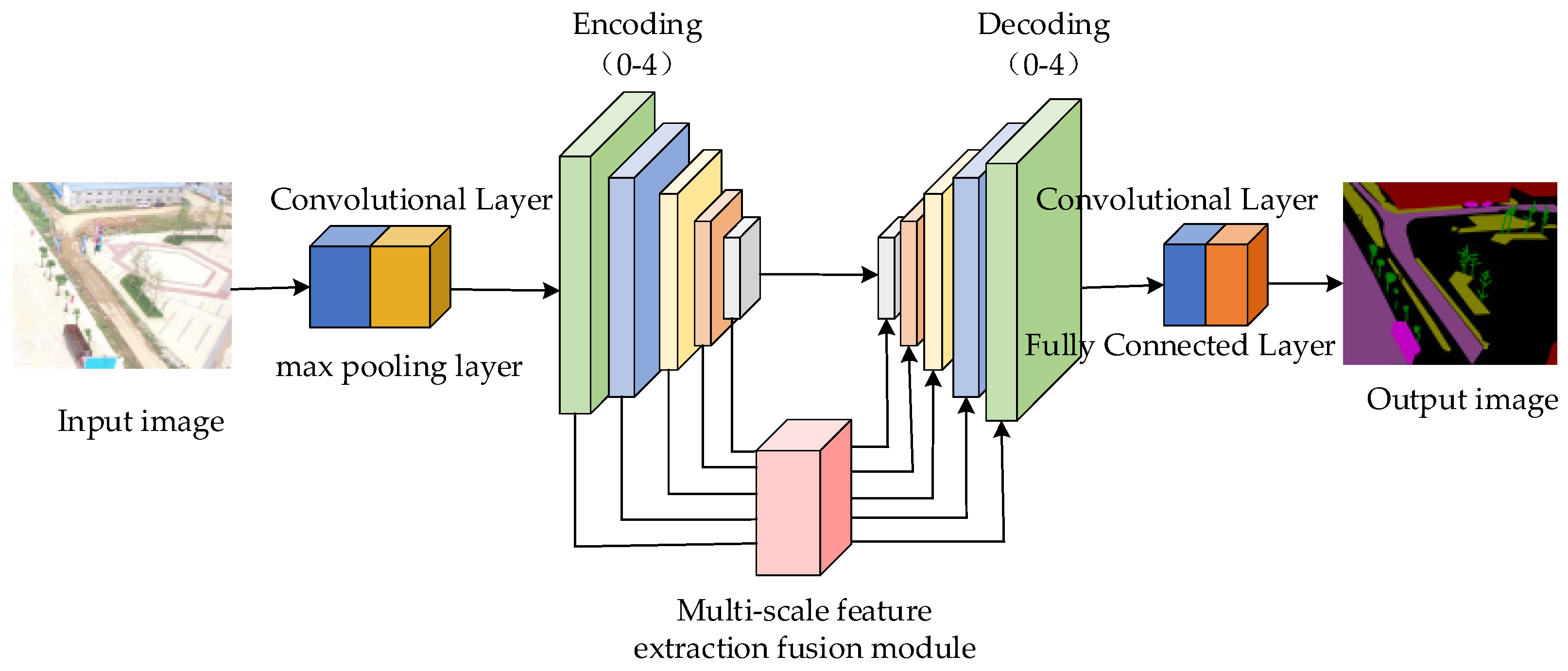
This paper uses a UAV multi-scale feature extraction integrated semantic segmentation network model. This model utilizes skip connections to transmit information between encoding and decoding layers. In the encoding layers, continuous downsampling of features extracts semantic features of a reasonable scale for targets [28]. On the other hand, the decoder gradually restores image clarity through a multi-scale feature extraction fusion module that performs continuous upsampling of features. Figure 1 illustrates the semantic segmentation network model with multi-scale feature extraction fusion.

In this paper, the network model introduces a multi-scale feature extraction and fusion module, utilizing multi-scale spatial feature extraction and multi-scale channel feature extraction to synergistically optimize the extracted complementary information, thereby learning more detailed feature representations. Specifically, after the input image is processed by the max-pooling layer and convolutional layer; then, it enters the encoding layer, where the encoder downsamples the image features and outputs the feature results. Next, before each upsampling layer’s decoder, a multi-scale feature extraction and fusion module is added. This module sends the processed image feature values into the decoding layer, where the decoder performs continuous upsampling to restore the image resolution. During this process, the image data are normalized and processed by the ReLU activation function each time it passes through a convolutional layer. Each upsampling layer doubles the feature dimensions while reducing the number of channels to half of the original. Additionally, the fused features output by the multi-scale feature extraction and fusion module are integrated with the encoded results of the same feature dimensions through skip connections. The skip connections use element-wise summation to merge corresponding elements.

The multi-scale feature extraction and fusion module presented in this paper effectively integrates detail and semantic information by combining the multi-scale channel feature extraction module with the multi-scale spatial feature extraction module. This approach incorporates a substantial amount of contextual information during the convolution process, addressing the issue of poor segmentation performance in shallow algorithmic models. Consequently, it enhances the recovery of finer segmentation details for various targets. The specific network structure of the module is illustrated in Figure 2.

The multi-scale feature extraction and fusion module is primarily divided into two components: the multi-scale channel feature extraction module and the multi-scale spatial feature extraction module. Here, ${\mathrm{X}}_{\mathrm{i}}\in {\mathrm{R}}^{\mathrm{C}\times \mathrm{H}\times \mathrm{W}}$ represents the features from the i-th stage of the encoder, with the feature channels and dimensions being C and $\mathrm{H}\times \mathrm{W}$, respectively. The operator $\oplus$ denotes element-wise multiplication, while $\oplus$ denotes element-wise addition. ${\mathrm{X}}_{\mathrm{i}}$ serves as the input to the multi-scale feature extraction and fusion module. The first component is the multi-scale channel feature extraction module. Initially, global average pooling is used to extract the primary channel information from the input features. This information is then input into a $1\times 1\times 1$ sized convolution layer to compress the convolution parameters. The sigmoid activation function is applied to normalize the input values, resulting in the multi-scale channel feature mask ${\mathrm{M}}_{\mathrm{ic}}$. The processed result is then multiplied with the original feature values to obtain the calibrated feature map ${\mathrm{U}}_{\mathrm{ic}1}$. The second component is the multi-scale spatial feature extraction module. This module derives spatial feature maps by leveraging spatial correlations among the input feature maps. Compared to multi-scale channel feature extraction, this component focuses more on the spatial information of the feature maps. The input feature map is sequentially processed through convolutional and activation layers, and the output from the sigmoid layer produces the activated multi-scale spatial feature mask ${\mathrm{M}}_{\mathrm{is}}$. Combining this with the original feature values yields the spatially calibrated feature map ${\mathrm{U}}_{\mathrm{is}1}$, thus completing the spatial information calibration process.

To mitigate the influence of background information on the results and address the issue of insufficient global context due to the shallow nature of the algorithm and thereby enhancing the segmentation capability of the model, context information can be incorporated during the decoding process. This involves further refinement of the features at each stage of model processing. In the multi-scale channel feature extraction and multi-scale spatial feature extraction modules, the input is the original feature block ${\mathrm{X}}_{\mathrm{i}}$. The weighted feature maps ${\mathrm{U}}_{\mathrm{ic}1}$ and ${\mathrm{U}}_{\mathrm{is}1}$ are balanced, and the feature weights are re-adjusted to obtain the corresponding weight maps ${\mathrm{U}}_{\mathrm{ic}}$ and ${\mathrm{U}}_{\mathrm{is}}$.

$${\mathrm{U}}_{\mathrm{ic}}={\mathrm{X}}_{\mathrm{i}}\oplus {\mathrm{U}}_{\mathrm{ic}1}={\mathrm{X}}_{\mathrm{i}}+{\mathrm{M}}_{\mathrm{ic}}\otimes {\mathrm{X}}_{\mathrm{i}}$$

(1)

$${\mathrm{U}}_{\mathrm{is}}={\mathrm{X}}_{\mathrm{i}}\oplus {\mathrm{U}}_{\mathrm{is}1}={\mathrm{X}}_{\mathrm{i}}+{\mathrm{M}}_{\mathrm{is}}\otimes {\mathrm{X}}_{\mathrm{i}}$$

(2)

A higher weight ratio indicates greater importance. Therefore, in this study, the range of values for the elements in ${\mathrm{M}}_{\mathrm{ic}}$ and ${\mathrm{M}}_{\mathrm{is}}$ is set from 0 to 1. When a value at a particular position approaches 1, the corresponding feature ${\mathrm{U}}_{\mathrm{i}}$ at that position increases. Conversely, when the value at a position approaches 0, the feature ${\mathrm{U}}_{\mathrm{i}}$ at that position remains close to the initial feature ${\mathrm{X}}_{\mathrm{i}}$. Consequently, after processing through the fusion module, the multi-scale spatial features are adapted to the multi-scale channel features while preserving the information of the original features. This approach enhances network learning and improves feature representation.

Furthermore, the output feature ${\mathrm{F}}_{\mathrm{i}}\in {\mathrm{R}}^{\mathrm{C}\times \mathrm{H}\times \mathrm{W}}$ from the multi-scale feature extraction and fusion module can be obtained using the following algorithm:

$${\mathrm{F}}_{\mathrm{i}}={\mathrm{f}}^{1\times 1}\left(\mathrm{concat}\left({\mathrm{U}}_{\mathrm{ic}},{\mathrm{U}}_{\mathrm{is}}\right)\right)$$

(3)

Here, concat denotes the concatenation operation performed along the channel dimension, and ${\mathrm{f}}^{1\times 1}$ represents a nonlinear transformation encompassing ReLU activation: a convolutional network with a stride of 1 and batch normalization. After this processing, the feature dimensions remain unchanged, while the total number of channels is reduced to half of the initial count.

Global features and detail features are effectively represented throughout the process. This not only significantly reduces the computational burden of the model, but also enhances the segmentation performance by connecting information across different layers, thereby achieving a richer global context with minimal computational cost. Additionally, incorporating initial feature maps from each stage further strengthens the global feature extraction capability. The multi-scale feature extraction and fusion module refines the output fused features, thereby enhancing the interaction between data. This, in turn, improves the analysis and prediction of features through the fusion of encoded stages, ultimately enhancing the segmentation characteristics.

The UAV aerial semantic map is obtained through the semantic segmentation network model mentioned in this section, as shown in Figure 3.

2.1.2. Task Point Acquisition

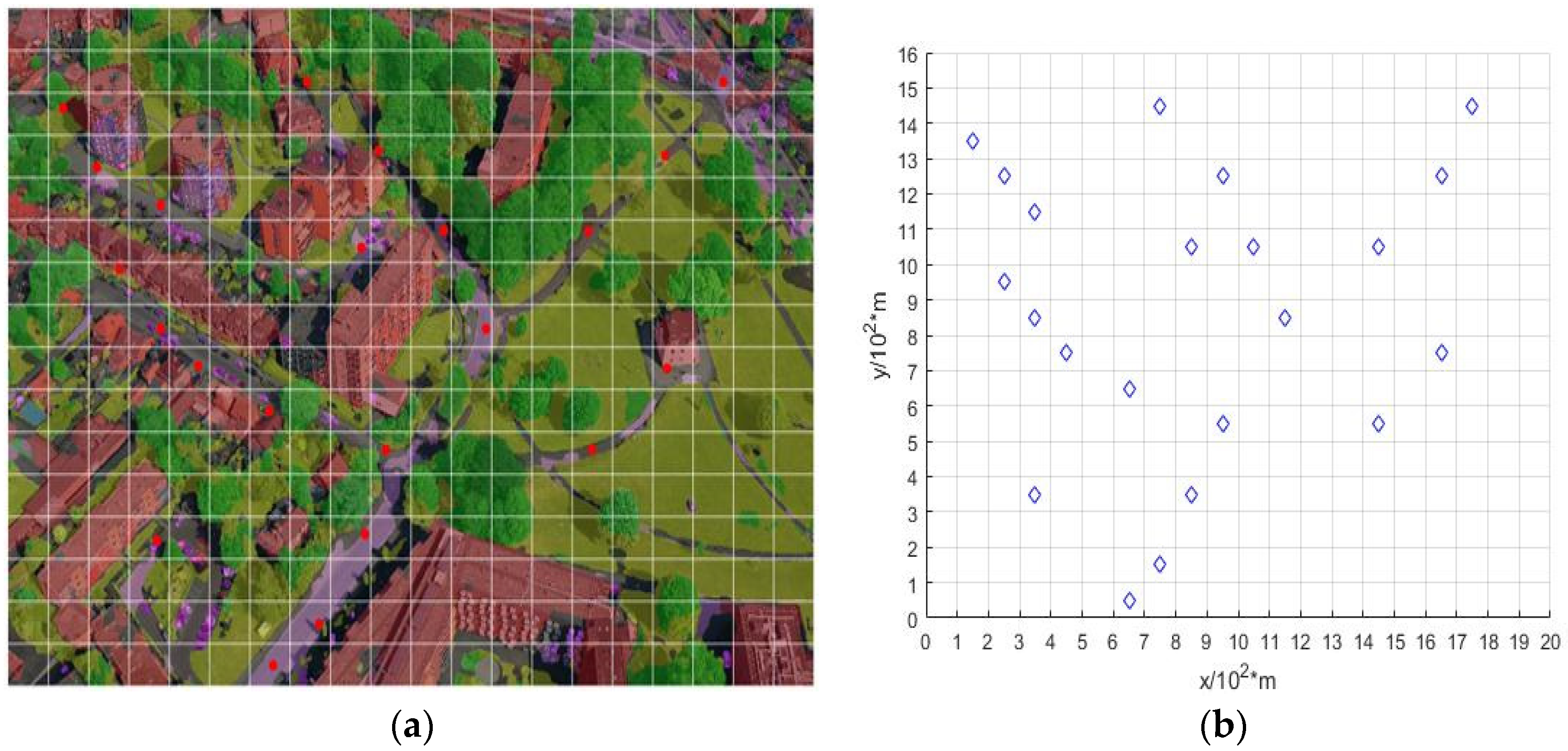
The UAV target reconnaissance mission area map is obtained through UAV aerial photography, as shown in Figure 4a. Using the multi-scale feature extraction fusion UAV semantic segmentation method proposed in the previous section, the task map with semantic information is acquired, as shown in Figure 4b.

How to extract sufficient and effective information from semantic segmentation results is the focus of this research. Assuming the UAV needs to search for vehicles, different probability values are assigned to different scenes in the semantic segmentation results based on the likelihood of vehicles appearing. For example, the probability of vehicles appearing on roads may be set to 0.8, while in vegetation areas it might be set to 0.3. Probability values in other locations are set according to the likelihood of vehicle presence. The final result is a UAV aerial semantic map that includes probability information for task points.

Based on the semantic map, regions requiring a focused search are identified, which may consist of multiple scattered areas. To efficiently search these areas, selective processing of search regions is conducted. Here, a sliding window approach is used to select essential points in the task area reconnaissance. The central point of high-probability areas serves as the center Oc, and essential points within the region are selected using a unit step length d, as shown in Equation (4).

$${(\mathrm{x},\mathrm{y})}_{\mathrm{k}+1}={(\mathrm{x},\mathrm{y})}_{{\mathrm{O}}_{\mathrm{c}}}+{{\displaystyle \sum }}^{ }\mathsf{\Delta }\mathrm{d}$$

(4)

By traversing all search regions and focusing on scattered small areas, selecting the networks with the highest probability as necessary search points provides guidance for UAV target reconnaissance, as shown in Figure 5.

2.2. UAV Motion Model

The motion state of the UAV is linear, and the trajectory of its movement can be expressed as follows:

$$\mathrm{F}\left(\mathrm{t}\right)={\left[\mathrm{x}\left(\mathrm{t}\right),\mathrm{y}\left(\mathrm{t}\right),\mathsf{\theta }\left(\mathrm{t}\right)\right]}^{\mathrm{T}}\in {\mathrm{R}}^2\times {\mathrm{S}}^1$$

(5)

In the above expression, x(t) and y(t) represent the position of the UAV in the inertial coordinate system as a function of time, while θ denotes the heading angle of the UAV relative to the X-axis. Given that the UAV aerial images do not include height information, this study considers only the UAV formation path planning problem in a two-dimensional coordinate system.

Assuming a constant motion speed of 1 for the UAV in the path planning model and a maximum curvature of $1/\mathsf{\gamma }$, the kinematic equations are expressed as follows:

$$\left(\begin{array}{c} \dot{\mathrm{x}}\\ \dot{\mathrm{y}}\\ \dot{\mathsf{\theta }}\end{array}\right)=\left(\begin{array}{c}\cos \mathsf{\theta }\\ \sin \mathsf{\theta }\\ \mathrm{c}/\mathsf{\gamma }\end{array}\right)$$

(6)

where θ ∈ [−1/γ, 1/γ], and the constant c is a control variable that varies with time for the UAV, with $|\mathrm{c}|\le 1$.

2.3. Task Assignment Model

The UAV path planning problem can be equated to the Multiple Traveling Salesman Problem (MTSP). Essentially, it involves assigning task points to individual UAVs within a formation based on the number of required task objectives and the constraints of the UAV’s flight characteristics. The goal is to find a path that meets the shortest travel distance requirements while ensuring the safety of the entire formation and the completion of all objectives [29]. To address this issue, we have developed a UAV formation path planning model. In this model, target demands and UAV characteristics serve as constraints, while target tasks and the UAV formation are the input variables, and the planned path for the UAV formation is the expected output.

2.3.1. Constructing the Objective Function

The total flight distance from the starting point of the UAV formation to its return is used as the optimization objective in the task assignment model. The model includes n task points, represented by the set $\mathrm{Target}=\left[\left({\mathrm{x}}_1,{\mathrm{y}}_1\right),\left({\mathrm{x}}_2,{\mathrm{y}}_2\right),\cdots ,\left({\mathrm{x}}_{\mathrm{n}},{\mathrm{y}}_{\mathrm{n}}\right)\right]$. The distance between two task points in the UAV formation’s mission planning path is given by the following equation:

$${\mathrm{d}}_{\mathrm{i},\mathrm{j}}=\sqrt{{\left({\mathrm{x}}_{\mathrm{i}}-{\mathrm{x}}_{\mathrm{j}}\right)}^2+{\left({\mathrm{y}}_{\mathrm{i}}-{\mathrm{y}}_{\mathrm{j}}\right)}^2}$$

(7)

In this study, the UAVs discussed are fixed-wing aircraft. The trajectory of these UAVs is constrained by curvature limits, meaning that the UAV formation follows a path with a certain range of curvature constraints [30]. Here, we simulate the UAV’s actual trajectory-changing capability using Dubins curves with a turning radius R.

$${\mathrm{d}}_{\mathrm{i},\mathrm{j}}=\mathrm{l}+\mathrm{r}+\mathrm{D}$$

(8)

In Equation (8), D represents the straight-line segment of the Dubins curve path, while l and r denote the left and right turning curve segments, respectively, in the Dubins curve path.

The optimization objective of the UAV formation task assignment model is to minimize the total travel distance of the UAV formation. According to Equation (8), the objective function can be expressed as follows:

$$\min \mathrm{L}={{\displaystyle \sum }}_{\mathrm{i}=1,\mathrm{j}=1,\mathrm{q}=1}^{\mathrm{n},\mathrm{n},\mathrm{m}}{\mathrm{d}}_{\mathrm{i},\mathrm{j}}{\ast \mathrm{k}}_{\mathrm{i},\mathrm{j},\mathrm{q}}$$

(9)

In Equation (9), ${\mathrm{k}}_{\mathrm{i},\mathrm{j},\mathrm{q}}$ represents whether UAV q has a planned task between target points i and j, where ${\mathrm{k}}_{\mathrm{i},\mathrm{j},\mathrm{q}}$ takes values of 0 or 1.

2.3.2. Constructing Constraint Conditions

Equation (10) represents the range constraints for UAV formation task execution, ensuring that the UAV formation flies within a specified range and thereby reducing flight paths.

$$\{\begin{array}{c}1\le {\mathrm{x}}_{\mathrm{i}}\le {\mathrm{x}}_{\max }\\ 1\le {\mathrm{y}}_{\mathrm{i}}\le {\mathrm{y}}_{\max }\end{array}$$

(10)

Equation (11) defines the flight characteristics constraint for UAV formation, incorporating UAV speed and maneuvering capabilities into the model.

$$\{\begin{array}{c}\mathrm{V}=1\\ -1/\mathsf{\gamma }\le \mathsf{\theta }\le 1/\mathsf{\gamma }\end{array}$$

(11)

Equation (12) represents the number of tasks assigned to each individual UAV, ensuring that each UAV is assigned at least k tasks. Equation (13) denotes the total number of tasks for the UAV formation, ensuring that all task points are allocated to the corresponding UAVs. Equation (14) specifies the number of UAVs assigned to each task point, with the requirement that each task point is assigned only once. Equation (15) is the criterion for determining the start and end points, where $\left({\mathrm{x}}_{\mathrm{w}},{\mathrm{y}}_{\mathrm{w}}\right)$ represents the coordinates of the last target point planned by an individual UAV, ensuring that each UAV’s starting and ending points are the same.

$${{\displaystyle \sum }}_{\mathrm{i}=1,\mathrm{j}=1,\forall \mathrm{q}\in \mathrm{m}}^{\mathrm{n},\mathrm{n}}{\mathrm{k}}_{\mathrm{i},\mathrm{j},\mathrm{q}}\ge \mathrm{k}$$

(12)

$${{\displaystyle \sum }}_{\mathrm{i}=1,\mathrm{j}=1,\mathrm{q}=1}^{\mathrm{n},\mathrm{n},\mathrm{m}}{\mathrm{k}}_{\mathrm{i},\mathrm{j},\mathrm{q}}=\mathrm{n}$$

(13)

$${{\displaystyle \sum }}_{\mathrm{i}\in \mathrm{n},\mathrm{j}\in \mathrm{n},\mathrm{q}=1}^{\mathrm{m}}{\mathrm{k}}_{\mathrm{i},\mathrm{j},\mathrm{q}}=1$$

(14)

$${\mathrm{d}}_{1,\mathrm{F}}=|\left({\mathrm{x}}_1,{\mathrm{y}}_1\right),\left({\mathrm{x}}_{\mathrm{F}},{\mathrm{y}}_{\mathrm{F}}\right)|=0,\forall \left(\mathrm{x},\mathrm{y}\right)\in \mathrm{Target}$$

(15)

3. Heading Angle Optimization Model

Let ${\mathsf{\phi }}_{\mathrm{x}}$, ${\mathsf{\phi }}_{\mathrm{y}}$, and ${\mathsf{\phi }}_{\mathsf{\theta }}$ be the parameters of the shortest path. Combining Equation (6) with the UAV motion equations and based on the theorem in optimal control theory, the Hamiltonian function for the UAV’s shortest path is constructed as follows [31]:

$$\mathrm{H}\left(\mathrm{x},\mathrm{y},\mathsf{\theta }\right)=1+{\mathsf{\phi }}_{\mathrm{x}}\cos \mathsf{\theta }+{\mathsf{\phi }}_{\mathrm{y}}\sin \mathsf{\theta }+{\mathsf{\phi }}_{\mathsf{\theta }}\mathrm{c}/\mathsf{\gamma }$$

(16)

Based on Equation (16) and applying Pontryagin’s maximum principle, the necessary conditions for the shortest path of a Dubins curve can be obtained [32].

$${\displaystyle \frac{\mathrm{d}}{\mathrm{dt}}}\left[\begin{array}{c}{\mathsf{\phi }}_{\mathrm{x}}\\ {\mathsf{\phi }}_{\mathrm{y}}\\ {\mathsf{\phi }}_{\mathsf{\theta }}\end{array}\right]=\left(\begin{array}{c}0\\ 0\\ {\mathsf{\phi }}_{\mathrm{x}}\mathrm{s}\mathrm{i}\mathrm{n}\mathsf{\theta }-{\mathsf{\phi }}_{\mathrm{y}}\mathrm{c}\mathrm{o}\mathrm{s}\mathsf{\theta }\end{array}\right)$$

(17)

The above equation indicates that ${\mathsf{\phi }}_{\mathrm{x}}$ and ${\mathsf{\phi }}_{\mathrm{y}}$ are constants over the interval [0, T]. From Equation (17), the following expression can be obtained:

$$\begin{array}{c}{\mathsf{\phi }}_{\mathrm{x}}\left({\mathrm{t}}_1^{+}\right)={\mathsf{\phi }}_{\mathrm{x}}\left({\mathrm{t}}_1^{-}\right)+{\mathrm{k}}_1\\ {\mathsf{\phi }}_{\mathrm{y}}\left({\mathrm{t}}_1^{+}\right)={\mathsf{\phi }}_{\mathrm{y}}\left({\mathrm{t}}_1^{-}\right)+{\mathrm{k}}_2\\ \begin{array}{c}{\mathsf{\phi }}_{\mathsf{\theta }}\left({\mathrm{t}}_1^{+}\right)={\mathsf{\phi }}_{\mathsf{\theta }}\left({\mathrm{t}}_1^{-}\right)\\ \mathrm{H}\left({\mathrm{t}}_1^{+}\right)=\mathrm{H}\left({\mathrm{t}}_1^{-}\right)\end{array}\end{array}$$

(18)

Figure 6 is a diagram of the optimal path. On the segments of the optimal path, ${\mathsf{\phi }}_{\mathsf{\theta }}=0$, and ${\mathrm{d}\mathsf{\phi }}_{\mathsf{\theta }}/\mathrm{dt}=0$. Substitute the above equation to solve the system of simultaneous equations and utilize the results from Equation (18) as follows:

$$\begin{array}{c}{\mathsf{\phi }}_{\mathrm{x}}=-\cos {\mathsf{\theta }}_0\\ {\mathsf{\phi }}_{\mathrm{y}}=-\sin {\mathsf{\theta }}_0\\ \begin{array}{c}{\mathsf{\phi }}_{\mathrm{x}}+{\mathrm{k}}_1=-\cos {\mathsf{\theta }}_1\\ {\mathsf{\phi }}_{\mathrm{y}}+{\mathrm{k}}_2=-\sin {\mathsf{\theta }}_1\end{array}\end{array}$$

(19)

From the above equation, it can be derived that ${\mathrm{k}}_1/{\mathrm{k}}_2=-\tan ({\mathsf{\theta }}_0+{\mathsf{\theta }}_1)/2$. The Hamiltonian function is continuous on the optimal arc at (${\mathrm{x}}_1,{\mathrm{y}}_1$), and therefore can be expressed as follows:

$$\begin{gathered} \underset{||\mathrm{c}||\le 1}{\mathrm{Min}}\left[1+{\mathsf{\phi }}_{\mathrm{x}}\cos {\mathsf{\theta }}_{\mathrm{m}}+{\mathsf{\phi }}_{\mathrm{y}}\sin {\mathsf{\theta }}_{\mathrm{m}}+{\mathsf{\phi }}_{\mathsf{\theta }}\mathrm{c}\right]= \\ \underset{||\mathrm{c}||\le 1}{\min }\left[1+\left({\mathsf{\phi }}_{\mathrm{x}}+{\mathrm{k}}_1\right)\cos {\mathsf{\theta }}_{\mathrm{m}}+{\mathsf{\phi }}_{\mathrm{y}}+{\mathrm{k}}_2\sin {\mathsf{\theta }}_{\mathrm{m}}+{\mathsf{\phi }}_{\mathsf{\theta }}\mathrm{c}\right] \end{gathered}$$

(20)

From the above equation, it can be seen that:

$${\mathrm{k}}_1\cos {\mathsf{\theta }}_{\mathrm{m}}+{\mathrm{k}}_2\sin {\mathsf{\theta }}_{\mathrm{m}}=0$$

(21)

From Equations (19) and (21), Equation (22) can be obtained.

$${\mathsf{\theta }}_{\mathrm{m}}={\displaystyle \frac{{\mathsf{\theta }}_0+{\mathsf{\theta }}_1}{2}}$$

(22)

The midpoint heading angle can be obtained through Equation (22), which allows for solving the coupled triangular equations to determine the optimal path heading angle parameters. This is challenging to describe with a general formula, as Ma et al.’s paper did not provide a formula that characterizes all possible geometric configurations [33]. Based on the horizon retreat principle, this paper presents a general formula for calculating the heading angle of the target point.

From Figure 7, the total flight path L between the three points after task planning can be obtained as follows:

$$\begin{array}{c}\mathrm{L}={\mathrm{L}}_{\mathrm{BD}}+{\mathrm{L}}_{\mathrm{EC}}+{\mathrm{S}}_{arc \mathrm{DE}}\\ >\mathrm{a}+\mathrm{b}+{\displaystyle \frac{\mathsf{\alpha }+\mathsf{\beta }}{180}}\mathsf{\pi }\mathrm{R}-2\mathrm{R}\sin {\displaystyle \frac{\mathsf{\alpha }}{2}}-2\mathrm{R}\sin {\displaystyle \frac{\mathsf{\beta }}{2}}\\ >\mathrm{a}+\mathrm{b}+{\displaystyle \frac{\mathsf{\alpha }+\mathsf{\beta }}{180}}\mathsf{\pi }\mathrm{R}-4\mathrm{R}\sin {\displaystyle \frac{\mathsf{\alpha }+\mathsf{\beta }}{4}}\cos {\displaystyle \frac{\mathsf{\alpha }-\mathsf{\beta }}{4}} \end{array}$$

(23)

In the above equation, a is the distance from the initial point B to the tangent point D, and b is the distance from the terminal point C to the tangent point E. From the equation, it is evident that the value of L depends on the values of α and β, as shown in Equation (24):

$$\mathrm{S}={\displaystyle \frac{\mathsf{\alpha }+\mathsf{\beta }}{180}}\mathsf{\pi }\mathrm{R}-4\mathrm{R}\sin {\displaystyle \frac{\mathsf{\alpha }+\mathsf{\beta }}{4}}\cos {\displaystyle \frac{\mathsf{\alpha }-\mathsf{\beta }}{4}}$$

(24)

From Equation (24), it can be seen that when α + β is minimized and α = β, the value of Equation (23) is minimized. From Figure 6, it is evident that when the center O is on the angle bisector of angle C, the total flight path L reaches its minimum value, given by ${\mathrm{L}}_{\min }=\mathrm{a}+\mathrm{b}+{\displaystyle \frac{\mathsf{\alpha }+\mathsf{\beta }}{180}}\mathsf{\pi }\mathrm{R}-4\mathrm{R}\sin {\displaystyle \frac{\mathsf{\alpha }+\mathsf{\beta }}{4}}$. The heading angle θ_m at the intermediate point (${\mathrm{x}}_1,{\mathrm{y}}_1$) is ${\mathsf{\theta }}_{\mathrm{m}}={\displaystyle \frac{{\mathsf{\theta }}_3+{\mathsf{\theta }}_2}{2}}$.

4. Improved Fuzzy C-Means Clustering Algorithm

Cluster algorithms are unsupervised learning methods that do not require prior knowledge of dataset information. They segment datasets into different clusters according to specific criteria, ensuring that data points within the same cluster share similar characteristics while maximizing differences between different clusters. This technology is widely applied in data mining, machine learning, pattern recognition, and artificial intelligence for information extraction and classification [34].

Cluster algorithms can be categorized into fuzzy clustering and hard clustering. Hard clustering algorithms such as the K-means algorithm follow the principle of either 0 or 1, meaning each data point belongs exclusively to one cluster [35]. While straightforward, hard clustering may overlook overlaps between data samples from different clusters. Fuzzy clustering, a soft clustering method, introduces the concepts of membership and membership functions, allowing data points to exhibit characteristics of multiple clusters. Based on membership values, data points are classified into clusters with higher likelihoods, making fuzzy clustering more suitable for real-life classification scenarios. The fuzzy C-means clustering algorithm is one of the most widely used clustering methods [36].

In a dataset D containing multiple data points x, there exists a corresponding relationship $\mathrm{U}\left(\mathrm{x}\right)\in \left[0, 1\right]$, where U is the fuzzy set of dataset D and $\mathrm{U}\left(\mathrm{x}\right)$ represents the membership function of data point x to dataset D. The membership function $\mathrm{U}\left(\mathrm{x}\right)$ ranges between 0 and 1: values closer to 1 indicate a higher degree of membership of data point x to fuzzy set U, while values closer to 0 indicate a lower degree of membership.

The fuzzy C-means clustering algorithm (FCM) uses a membership matrix $\mathrm{U}=\left[{\mathrm{u}}_{\mathrm{ij}}\right]$ to represent the degree to which each data point belongs to each cluster. The objective function is as follows.

$$\mathrm{J}\left(\mathrm{U},\mathrm{C}\right)={{\displaystyle \sum }}_{\mathrm{j}=1}^{\mathrm{N}}{{\displaystyle \sum }}_{\mathrm{i}=1}^{\mathrm{M}}{\left({\mathrm{u}}_{\mathrm{ij}}\right)}^{\mathrm{k}}\ast {||{\mathrm{c}}_{\mathrm{i}}-{\mathrm{x}}_{\mathrm{j}}||}^2$$

(25)

In Equation (25), N is the size of dataset D, M is the number of cluster centers, k is the weighting exponent (typically set to 2), and ${\mathrm{c}}_{\mathrm{i}}$ represents the coordinates of cluster centers. Equation (25) calculates the membership degree of data points, where minimizing its value yields optimal results.

$$\min \left\{\mathrm{J}\left(\mathrm{U},\mathrm{C}\right)\right\}=\min \left\{{{\displaystyle \sum }}_{\mathrm{j}=1}^{\mathrm{N}}{{\displaystyle \sum }}_{\mathrm{i}=1}^{\mathrm{M}}{\left({\mathrm{u}}_{\mathrm{ij}}\right)}^{\mathrm{k}}\ast ||{\mathrm{c}}_{\mathrm{i}}-{{\mathrm{x}}_{\mathrm{j}}||}^2\right\}=\min \left\{{{\displaystyle \sum }}_{\mathrm{i}=1}^{\mathrm{M}}{\left({\mathrm{u}}_{\mathrm{ij}}\right)}^{\mathrm{k}}\ast ||{\mathrm{c}}_{\mathrm{i}}-{{\mathrm{x}}_{\mathrm{j}}||}^2\right\}$$

(26)

Equation (26) satisfies the constraint conditions ${{\displaystyle \sum }}_{\mathrm{i}=1}^{\mathrm{M}}{\mathrm{u}}_{\mathrm{ij}}=1$.

$$\mathrm{F}={{\displaystyle \sum }}_{\mathrm{i}=1}^{\mathrm{M}}{\left({\mathrm{u}}_{\mathrm{ij}}\right)}^{\mathrm{k}}\ast ||{\mathrm{c}}_{\mathrm{i}}-{{\mathrm{x}}_{\mathrm{j}}||}^2+\mathsf{\lambda }\left({{\displaystyle \sum }}_{\mathrm{i}=1}^{\mathrm{M}}{\mathrm{u}}_{\mathrm{ij}}-1\right)$$

(27)

$${\displaystyle \frac{\partial \mathrm{F}}{\partial {\mathrm{u}}_{\mathrm{ij}}}}={{\mathrm{m}\ast \mathrm{u}}_{\mathrm{ij}}}^{\mathrm{k}-1}\ast ||{\mathrm{c}}_{\mathrm{i}}-{{\mathrm{x}}_{\mathrm{j}}||}^2-\mathsf{\lambda }=0\Rightarrow { \mathrm{u}}_{\mathrm{ij}}={\left({\displaystyle \frac{\mathsf{\lambda }}{\mathrm{k}}}\right)}^{{\displaystyle \frac{1}{\mathrm{k}-1}}}{\left({\displaystyle \frac{\mathsf{\lambda }}{||{\mathrm{c}}_{\mathrm{i}}-{{\mathrm{x}}_{\mathrm{j}}||}^2}}\right)}^{{\displaystyle \frac{1}{\mathrm{k}-1}}}$$

(28)

$${\displaystyle \frac{\partial \mathrm{F}}{\partial \mathsf{\lambda }}}={{\displaystyle \sum }}_{\mathrm{i}=1}^{\mathrm{M}}{\mathrm{u}}_{\mathrm{ij}}-1=0$$

(29)

Substitute Equation (29) into Equation (28) to obtain Equation (30).

$${{\displaystyle \sum }}_{\mathrm{i}=1}^{\mathrm{M}}{\left({\displaystyle \frac{\mathsf{\lambda }}{\mathrm{k}}}\right)}^{{\displaystyle \frac{1}{\mathrm{k}-1}}}{\left({\displaystyle \frac{\mathsf{\lambda }}{||{\mathrm{c}}_{\mathrm{i}}-{{\mathrm{x}}_{\mathrm{j}}||}^2}}\right)}^{{\displaystyle \frac{1}{\mathrm{k}-1}}}-1=0⟹{\left({\displaystyle \frac{\mathsf{\lambda }}{\mathrm{k}}}\right)}^{{\displaystyle \frac{1}{\mathrm{k}-1}}}={\displaystyle \frac{1}{{{\displaystyle \sum }}_{\mathrm{i}=1}^{\mathrm{M}}{\left(\frac{\mathsf{\lambda }}{||{\mathrm{c}}_{\mathrm{i}}-{{\mathrm{x}}_{\mathrm{j}}||}^2}\right)}^{\frac{1}{\mathrm{k}-1}}}}$$

(30)

Substituting Equation (30) into Equation (28) yields the membership matrix U.

$${\mathrm{u}}_{\mathrm{ij}}={\displaystyle \frac{1}{{{\displaystyle \sum }}_{\mathrm{j}=1}^{\mathrm{N}}{\left(\frac{||{\mathrm{c}}_{\mathrm{i}}-{{\mathrm{x}}_{\mathrm{i}}||}^2}{||{\mathrm{c}}_{\mathrm{i}}-{{\mathrm{x}}_{\mathrm{j}}||}^2}\right)}^{-\frac{1}{\mathrm{k}-1}}}}$$

(31)

Taking the derivative of Equation (21) with respect to the cluster center c, we obtain the following equation:

$${\displaystyle \frac{\partial \mathrm{J}\left(\mathrm{U},\mathrm{C}\right)}{\partial {\mathrm{c}}_{\mathrm{i}}}}={\displaystyle \frac{{{\displaystyle \sum }}_{\mathrm{j}=1}^{\mathrm{N}}{{\displaystyle \sum }}_{\mathrm{i}=1}^{\mathrm{M}}{\left({\mathrm{u}}_{\mathrm{ij}}\right)}^{\mathrm{k}}\ast \partial ||{\mathrm{c}}_{\mathrm{i}}-{{\mathrm{x}}_{\mathrm{j}}||}^2}{\partial {\mathrm{c}}_{\mathrm{i}}}}$$

(32)

$$||{\mathrm{c}}_{\mathrm{i}}-{{\mathrm{x}}_{\mathrm{j}}||}^2=||{\mathrm{c}}_{\mathrm{i}}-{{\mathrm{x}}_{\mathrm{j}}||}_{\mathrm{A}}={\left({\mathrm{c}}_{\mathrm{i}}-{\mathrm{x}}_{\mathrm{j}}\right)}^{\mathrm{T}}\mathrm{A}\left({\mathrm{c}}_{\mathrm{i}}-{\mathrm{x}}_{\mathrm{j}}\right)$$

(33)

In Equation (33), A represents the weight. Substituting Equation (33) into Equation (32), we obtain the following equation:

$${\displaystyle \frac{\partial \mathrm{J}\left(\mathrm{U},\mathrm{C}\right)}{\partial {\mathrm{c}}_{\mathrm{i}}}}={{\displaystyle \sum }}_{\mathrm{j}=1}^{\mathrm{N}}{{\mathrm{u}}_{\mathrm{ij}}}^{\mathrm{k}}{\displaystyle \frac{\partial {\left({\mathrm{c}}_{\mathrm{i}}-{\mathrm{x}}_{\mathrm{j}}\right)}^{\mathrm{T}}\mathrm{A}\left({\mathrm{c}}_{\mathrm{i}}-{\mathrm{x}}_{\mathrm{j}}\right)}{\partial {\mathrm{c}}_{\mathrm{i}}}}={{\displaystyle \sum }}_{\mathrm{j}=1}^{\mathrm{N}}{{\mathrm{u}}_{\mathrm{ij}}}^{\mathrm{k}}\left(2\mathrm{A}\ast \left({\mathrm{c}}_{\mathrm{i}}-{\mathrm{x}}_{\mathrm{j}}\right)\right)=0$$

(34)

From Equation (34), the cluster center c can be obtained, which is as follows:

$$2\mathrm{A}\ast \left({{\displaystyle \sum }}_{\mathrm{j}=1}^{\mathrm{N}}{{\mathrm{u}}_{\mathrm{ij}}}^{\mathrm{k}}{\mathrm{c}}_{\mathrm{i}}-{{\displaystyle \sum }}_{\mathrm{j}=1}^{\mathrm{N}}{{\mathrm{u}}_{\mathrm{ij}}}^{\mathrm{k}}{\mathrm{x}}_{\mathrm{j}}\right)=0⟹{\mathrm{c}}_{\mathrm{i}}={\displaystyle \frac{{{\displaystyle \sum }}_{\mathrm{j}=1}^{\mathrm{N}}{{\mathrm{u}}_{\mathrm{ij}}}^{\mathrm{k}}{\mathrm{x}}_{\mathrm{j}}}{{{\displaystyle \sum }}_{\mathrm{j}=1}^{\mathrm{N}}{{\mathrm{u}}_{\mathrm{ij}}}^{\mathrm{k}}}}$$

(35)

In Equations (31) and (35), it is observed that the values of the membership matrix U and cluster centers c are interdependent. Therefore, in the iterative process of the fuzzy C-means clustering algorithm, both parameters are calculated iteratively and updated continuously until the objective function $\mathrm{J}\left(\mathrm{U},\mathrm{C}\right)$ reaches convergence accuracy. The final values are determined by the membership matrix U and cluster centers c. However, at the beginning of the algorithm iteration, there are no initial values for U and c. Hence, it is necessary to set initial values for the membership matrix U and cluster centers c, as these parameters dictate the processing results and convergence speed of the fuzzy clustering algorithm. This paper proposes a method for selecting initial values for the membership matrix and cluster centers based on the fuzzy C-means clustering algorithm.

The steps to determine the initial membership matrix are as follows:

(1)

Input task point coordinates, initial UAV coordinates, number of UAVs, and search radius.

(2)

Randomly generate an initial membership matrix U.

(3)

Use the UAV position as the center and a radius R as the search radius to determine the task points within the search radius, as shown in Figure 8. Green dots are identified task points within the search radius, blue dots are task points to be identified outside the search radius.

(4)

Initially classify the task points by assigning those located within the UAV search radius and exclusively belonging to one cluster to the UAV search radius cluster. Classify task points within the overlap areas and outside the search radius as clusters to be classified.

(5)

Modify the initial membership matrix U by updating the membership values of the classified task points from step (3) to correspond to their respective clusters, as shown in Figure 9.

(6)

Output the modified initial membership matrix U.

In the cooperative task allocation model, there exists a formation set of UAVs, ${\mathrm{U}}_{\mathrm{uav}}=\left({\mathrm{u}}_1,{\mathrm{u}}_2\cdots {\mathrm{u}}_{\mathrm{n}-1},{\mathrm{u}}_{\mathrm{n}}\right)$, and this set is in the coordinate system ${\mathrm{S}}_{\mathrm{uav}}={\left[{\mathrm{x}}_{\mathrm{i}},{\mathrm{y}}_{\mathrm{i}}\right]}_{\mathrm{M}}$. The set of task points is $\mathrm{T}={\left[{\mathrm{x}}_{\mathrm{i}},{\mathrm{y}}_{\mathrm{i}}\right]}_{\mathrm{N}}$, where M is much smaller than N. Let matrix D represent the Euclidean distances between task points; the distance matrix D can be obtained as follows:

$${\mathrm{D}}_{\mathrm{ij}}=||{\mathrm{T}}_{\mathrm{i}}-{{\mathrm{T}}_{\mathrm{j}}||}^2$$

(36)

$$\mathrm{D}=\left[\begin{array}{ccc}\begin{array}{cc}\begin{array}{c}{\mathrm{D}}_{11}\\ {\mathrm{D}}_{21}\end{array}& \begin{array}{c}{\mathrm{D}}_{12}\\ {\mathrm{D}}_{22}\end{array}\end{array}& \cdots & \begin{array}{c}{\mathrm{D}}_{\mathrm{N}-1}\\ {\mathrm{D}}_{2\left(\mathrm{N}-1\right)}\end{array}\\ ⋮& \ddots & ⋮\\ \begin{array}{cc}{\mathrm{D}}_{\mathrm{N}1}& {\mathrm{D}}_{\mathrm{N}2}\end{array}& \cdots & {\mathrm{D}}_{\mathrm{m}\left(\mathrm{N}-1\right)}\end{array}\right]$$

(37)

Sum each row of matrix D to obtain Equation (38), which represents the total distance from the i-th task point to all other points.

$$\mathrm{G}=\left[\begin{array}{c}{{\displaystyle \sum }}^{ }{\mathrm{D}}_{1\mathrm{i}}\\ {{\displaystyle \sum }}^{ }{\mathrm{D}}_{2\mathrm{i}}\\ \begin{array}{c}⋮\\ {{\displaystyle \sum }}^{ }{\mathrm{D}}_{\mathrm{Ni}}\end{array}\end{array}\right]$$

(38)

The steps for selecting the cluster center ccc are as follows:

(1)

Input the initial membership matrix U, initial UAV coordinates, distance matrix D, total distance matrix G, and convergence threshold η.

(2)

From the initial UAV coordinates, construct the distance matrix D for other points relative to the UAV. Perform a minimum element search on matrix D to find the point closest to the initial UAV position and use this point as the initial cluster center c.

(3)

Merge the cluster containing the cluster center c with the cluster to be determined. Calculate its distance matrix G according to Equation (37) and select the task point corresponding to the minimum element of matrix G as the new cluster center.

(4)

Use the cluster center obtained in the previous step as the new cluster center and repeat step 2 until the objective function is less than the threshold.

(5)

Repeat the above steps to find the cluster center ccc for each cluster.

(6)

Output the cluster center c for all clusters.

5. Results and Analysis

In Section 2 and Section 3, we introduced an optimized heading angle algorithm and a UAV formation task allocation model based on an improved fuzzy C-means clustering algorithm. To validate the effectiveness of our proposed algorithms, we simulated the scenario of a single UAV searching multiple task points within a small area of 1 × 1 km². Additionally, we conducted simulations in two larger areas of 10 × 10 km² and 20 × 20 km², where target points were randomly distributed with quantities of 50 and 100. Task points were classified according to different algorithms.

Experiment 1: A single UAV performed path planning for 10 task points within a 1 × 1 km² area. The planning paths were compared using the ETSP model, AA algorithm, 2-opt algorithm, and optimized heading angle algorithm. The efficiency of these four algorithms was evaluated and compared.

Figure 10 illustrates the planned paths using the ETSP model, AA algorithm, 2-opt algorithm, and optimized heading angle algorithm. The simulation focused on path planning for a drone within a small area. Due to the inherent characteristics of the drone and varying heading angles, different algorithms yielded different planning results. The figure clearly shows that the path planned using the ETSP model is the shortest, which is suitable for rotary-wing drones but does not align with the actual conditions for fixed-wing drones.

Table 1. Initial coordinate settings for the UAV.

UAV Serial Number	Coordinate	UAV Speed (Relative Map Scale)	Minimum Turning Radius
UAV 1	5, 0	1	100 m

shows the initial parameters of the UAV.

Table 2. Total path length planning for 10 task points within a 1 km × 1 km area using different algorithms.

	ETSP	AA Algorithm	2-Opt Algorithm	Optimized Heading Angle Algorithm
Total distance (km)	30.8076	59.0470	35.2839	32.9486

shows the total travelling distance for different algorithms to plan the paths. The path length for the classic AA algorithm is the longest, totaling 59.0470 km. The proposed optimized heading angle algorithm results in a total path length that is only 6.9% longer than the shortest path obtained with the ETSP model and 6.6% longer than that from the 2-opt algorithm. The proposed optimized heading angle algorithm aligns with practical requirements.

Experiment 2: Four UAVs were used to classify and process 100 task points within a 20 km × 20 km area. The task planning efficiency was compared among the improved FCM algorithm, original FCM algorithm, and MTSP model.

Table 3. Initial coordinate settings for the UAV formation.

UAV Serial Number	Coordinate	UAV Speed (Relative Map Scale)	Minimum Turning Radius
UAV 1	0, 0	1	100 m
UAV 2	20, 0	1	100 m
UAV 3	20, 20	1	100 m
UAV 4	0, 20	1	100 m

shows the initial coordinates of the UAV.

Figure 11 shows the classification results of task points using the original FCM algorithm, improved FCM algorithm, and MTSP model. From the Figure 11, it is evident that the classification based on the MTSP model is notably more chaotic. Compared to the original FCM algorithm, the improved FCM algorithm demonstrates greater flexibility in classifying boundary task points.

Table 4. The distribution of task points in each cluster of 100 task points within a 20 km × 20 km area using different classification algorithms.

Algorithm	UAV 1 Cluster	UAV 2 Cluster	UAV 3 Cluster	UAV 4 Cluster
Original FCM	20	27	27	26
Improved FCM	19	25	32	24
MTSP model	25	23	26	26

presents the distribution of task points in each cluster within the 20 × 20 area using different classification algorithms. It is observed that in the UAV3 cluster region, there is a higher density of task point distribution, and the improved FCM algorithm shows more refined classification in this area.

Table 5. Total path length planning for 100 task points within a 20 km × 20 km area using different classification algorithms.

	Original FCM	Improved FCM	MTSP Model
Total distance (km)	186.0763	177.1994	193.9360
Number of large-angle turns	46	38	51

displays the total path lengths planned by the different algorithms. The improved FCM algorithm has the shortest distance, with a 4.8% improvement over the original FCM algorithm and an 8.6% improvement over the MTSP model. Additionally, the improved FCM classification algorithm proposed in this paper results in the shortest number of large-angle turns (>30°), with only 38 turns.

Experiment 3: Four UAVs were used to classify and process 50 task points within a 10 km × 10 km area. Task planning efficiency was compared among the improved FCM algorithm, original FCM algorithm, and MTSP model.

Figure 12 depicts the classification results of task points using the original FCM algorithm, improved FCM algorithm, and MTSP model within a smaller area. In this experiment, the number of task points was reduced from 100 to 50. It is evident that the MTSP model shows noticeable improvement in classification compared to the larger-scale experiment, yet still falls short of the classification effectiveness achieved by the improved FCM algorithm.

Table 6. The distribution of task points in each cluster of 50 task points within a 10 × 10 km area using different classification algorithms.

Algorithm	UAV 1 Cluster	UAV 2 Cluster	UAV 3 Cluster	UAV 4 Cluster
Original FCM	10	15	15	10
Improved FCM	11	13	16	10
MTSP model	10	14	12	14

presents the distribution of task points in each cluster using different algorithms, while

Table 7. Total path length planning for 50 task points within a 10 km × 10 km area using different classification algorithms.

	Original FCM	Improved FCM	MTSP Model
Total distance	78.0042	73.5801	76.6597
Number of large-angle turns	25	23	25

shows the total planned path lengths. The data in Table 7 indicate that the improved FCM algorithm exhibits the fewest large-angle turns, totaling 25, and also has the shortest total path length among the three algorithms, with improvements of 5.7% and 4% over the other two algorithms, respectively.

Experiment 4: Four UAVs were used to classify and search 100 task points within a 20 km × 20 km area. Path planning was prearranged, comparing the search efficiency of the optimized heading angle model, AA algorithm, and ETSP model for UAV formation path planning.

Figure 13 shows the trajectory planning for multiple UAVs and multiple target points using different algorithms. It is evident from the figure that the optimized heading angle model algorithm successfully completes the path planning task for multiple UAVs and targets. It avoids the circling around in UAV3 cluster as seen with the AA algorithm, resulting in smoother planned trajectories that better meet our practical needs. Moreover, the total mileage of the path planned by the optimized heading angle model is the shortest. As calculated in

Table 8. Total path length planning for 100 task points within a 20 km × 20 km area using different algorithms.

	Optimized Heading Angle Model	AA Algorithm	ETSP Model
Total distance	179.9206	185.5463	177.1994

, using the optimized heading angle model provides a minimum improvement of 2.1% in multi-task and multi-UAV path planning models.

6. Conclusions

In addressing the problem of shortest path planning for UAV formations guided by semantic map information, this paper employs a semantic segmentation network model based on multi-scale feature extraction for UAVs, obtaining a UAV aerial semantic map enriched with environmental information. Building upon the semantic map, we propose an algorithm for optimizing heading angles using fuzzy clustering for UAV formation path planning. A general formula for computing the optimal heading angle is provided. In Section 5, experimental results comparing the optimized heading angle model with AA algorithm and ETSP model for task allocation path planning demonstrate that our proposed optimized heading angle model achieves a minimum 4.1% improvement in travel distance and reduces major turning angles by 17.4%.

For large-scale UAV formation planning, we enhanced the FCM algorithm by modifying the initial membership matrix U and clustering centers based on the initial positions of the UAVs. Results from Experiment 2 and Experiment 3 indicate that our enhanced C-means clustering algorithm effectively classifies task point sets within different task ranges. The planned trajectories post-classification shows an 8.6% improvement over the original FCM algorithm and MTSP model, aligning with the design requirements of this paper.

However, during the task point classification process, distance constraints between task points were not considered, potentially resulting in suboptimal trajectory planning in certain individual cases. Therefore, future work will focus on a more detailed study of constraint conditions in the model classification phase.

References

1. Khuwaja, A.A.; Chen, Y.; Zhao, N.; Alouini, M.-S.; Dobbins, P. A Survey of Channel Modeling for UAV Communications. IEEE Commun. Surv. Tutor. 2018, 20, 2804–2821. [Google Scholar] [CrossRef]
2. McEnroe, P.; Wang, S.; Liyanage, M. A Survey on the Convergence of Edge Computing and AI for UAVs: Opportunities and Challenges. IEEE Internet Things J. 2022, 9, 15435–15459. [Google Scholar] [CrossRef]
3. Zhong, Y.; Wang, X.; Xu, Y.; Wang, S.; Jia, T.; Hu, X.; Zhao, J.; Wei, L.; Zhang, L. Mini-UAV-Borne Hyperspectral Remote Sensing: From Observation and Processing to Applications. IEEE Geosci. Remote Sens. Mag. 2018, 6, 46–62. [Google Scholar] [CrossRef]
4. Nex, F.; Armenakis, C.; Cramer, M.; Cucci, D.A.; Gerke, M.; Honkavaara, E.; Kukko, A.; Persello, C.; Skaloud, J. UAV in the advent of the twenties: Where we stand and what is next. ISPRS J. Photogramm. Remote Sens. 2022, 184, 215–242. [Google Scholar] [CrossRef]
5. Zhang, Z.; Zhu, L. A Review on Unmanned Aerial Vehicle Remote Sensing: Platforms, Sensors, Data Processing Methods, and Applications. Drones 2023, 7, 398. [Google Scholar] [CrossRef]
6. Rahim, S.; Razaq, M.M.; Chang, S.Y.; Peng, L. A reinforcement learning-based path planning for collaborative UAVs. In Proceedings of the 37th ACM/SIGAPP Symposium on Applied Computing (SAC ’22), Virtual, 25–29 April 2022; Association for Computing Machinery: New York, NY, USA, 2022; pp. 1938–1943. [Google Scholar]
7. Li, Y.; Zhang, X.; Zhu, Y.; Gao, Z. A UAV Path Planning Method in Three-Dimensional Urban Airspace based on Safe Reinforcement Learning. In Proceedings of the 2023 IEEE/AIAA 42nd Digital Avionics Systems Conference (DASC), Barcelona, Spain, 1–5 October 2023; pp. 1–7. [Google Scholar] [CrossRef]
8. Lippi, M.; Marino, A. A Mixed-Integer Linear Programming Formulation for Human Multi-Robot Task Allocation. In Proceedings of the 2021 30th IEEE International Conference on Robot & Human Interactive Communication (RO-MAN), Vancouver, BC, Canada, 8–12 August 2021; pp. 1017–1023. [Google Scholar] [CrossRef]
9. Berger, J.; Lo, N. An innovative multi-agent search-and-rescue path planning approach. Comput. Oper. Res. 2015, 53, 24–31. [Google Scholar] [CrossRef]
10. Liang, G.; Kang, Y.-H.; Xing, Z.; Yin, G.Y. UAV Cooperative Multi-task Assignment Based on Discrete Particle Swarm Optimization Algorithm. Comput. Simul. 2018, 35, 22–28. (In Chinese) [Google Scholar]
11. Wang, J.; Guo, J.; Murong, Z. Minimum-risk problem of unmanned aerial vehicle task allocation with expert belief degree. Control. Decis. 2019, 34, 2036–2040. (In Chinese) [Google Scholar]
12. Gao, L.; Han, Z.; Hong, D.; Zhang, B.; Chanussot, J. CyCU-Net: Cycle-consistency unmixing network by learning cascaded autoencoders. IEEE Trans. Geosci. Remote Sens. 2022, 60, 5503914. [Google Scholar] [CrossRef]
13. Gao, L.; Li, J.; Zheng, K.; Jia, X. Enhanced autoencoders with attention-embedded degradation learning for unsupervised hyperspectral image super-resolution. IEEE Trans. Geosci. Remote Sens. 2023, 61, 5509417. [Google Scholar] [CrossRef]
14. Su, Y.; Gao, L.; Jiang, M.; Plaza, A.; Sun, X.; Zhang, B. NSCKL: Normalized spectral clustering with kernel-based learning for semisupervised hyperspectral image classification. IEEE Trans. Cybern. 2023, 53, 6649–6662. [Google Scholar] [CrossRef]
15. Yao, P.; Wang, H.; Ji, H. Multi-UAVs tracking target in urban environment by model predictive control and improved grey wolf optimizer. Aerosp. Sci. Technol. 2016, 55, 131–143. [Google Scholar] [CrossRef]
16. Riehl, J.R.; Collins, G.E.; Hespanha, J.P. Cooperative search by UAV teams: A model predictive approach using dynamic graphs. IEEE Trans. Aerosp. Electron. Syst. 2011, 47, 2637–2656. [Google Scholar] [CrossRef]
17. Huang, L.; Qu, H.; Ji, P.; Liu, X.; Fan, Z. A novel coordinated path planning method using k-degree smoothing for multi-UAVs. Appl. Soft Comput. 2016, 48, 182–192. [Google Scholar] [CrossRef]
18. Wu, Y.; Wu, S.; Hu, X. Cooperative path planning of UAVs & UGVs for a persistent surveillance task in urban environments. IEEE Internet Things J. 2021, 8, 4906–4919. [Google Scholar]
19. Jiang, Y.; Bai, T.; Wang, D.; Wang, Y. Coverage Path Planning of UAV Based on Linear Programming—Fuzzy C-Means with Pigeon-Inspired Optimization. Drones 2024, 8, 50. [Google Scholar] [CrossRef]
20. Zheng, L.; Zhang, P.; Tan, J.; Chen, M. The UAV Path Planning Method Based on Lidar. In Intelligent Robotics and Applications; Yu, H., Liu, J., Liu, L., Ju, Z., Liu, Y., Zhou, D., Eds.; ICIRA 2019; Lecture Notes in Computer Science; Springer: Cham, Switzerland, 2019; Volume 11742. (In Chinese) [Google Scholar]
21. Liang, X.; Meng, G.; Luo, H.; Chen, X. Dynamic path planning based on improved boundary value problem for unmanned aerial vehicle. Clust. Comput. 2016, 19, 2087–2096. [Google Scholar] [CrossRef]
22. Hao, Q.; Zhao, H.; Huang, H.; Gui, G.; Ohtsuki, T.; Adachi, F. Deep Reinforcement Learning Aided Online Trajectory Optimization of Cellular-Connected UAVs with Offline Map Reconstruction. In Proceedings of the 2023 IEEE 97th Vehicular Technology Conference (VTC2023-Spring), Florence, Italy, 20–23 June 2023; pp. 1–5. [Google Scholar]
23. Liu, L.; Wang, D.; Yu, J.; Yao, P.; Zhong, C.; Fu, D. A Hierarchical Heuristic Architecture for Unmanned Aerial Vehicle Coverage Search with Optical Camera in Curve-Shape Area. Remote Sens. 2024, 16, 1502. [Google Scholar] [CrossRef]
24. Mo, Y.; Wu, Y.; Yang, X.; Liu, F.; Liao, Y. Review the state-of-the-art technologies of semantic segmentation based on deep learning. Neurocomputing 2022, 7, 493. [Google Scholar] [CrossRef]
25. Xie, Y.; Tian, J.; Zhu, X.X. Linking Points With Labels in 3D: A Review of Point Cloud Se-mantic Segmentation. IEEE Geosci. Remote Sens. Mag. 2020, 8, 38–59. [Google Scholar] [CrossRef]
26. Cheng, J.; Deng, C.; Su, Y.; An, Z.; Wang, Q. Methods and datasets on semantic seg-mentation for Unmanned Aerial Vehicle remote sensing images: A review. ISPRS J. Photogramm. Remote Sens. 2024, 211, 1–34. [Google Scholar] [CrossRef]
27. Park, J.; Yoo, H.; Wang, Y. Drivable Dirt Road Region Identification Using Image and Point Cloud Semantic Segmentation Fusion. IEEE Trans. Intell. Transp. Syst. 2022, 23, 13203–13216. [Google Scholar] [CrossRef]
28. Wei, D.; Wang, H. MFFLNet: Lightweight semantic segmentation network based on multi-scale feature fusion. Multim. Tools Appl. 2023, 83, 30073–30093. [Google Scholar]
29. Liu, L.; Wang, X.; Yang, X.; Liu, H.; Li, J.; Wang, P. Path planning techniques for mobile robots: Review and prospect. Expert Syst. Appl. 2023, 227, 120254. [Google Scholar] [CrossRef]
30. Sujit, P.B.; Saripalli, S.; Sousa, J.B. Unmanned Aerial Vehicle Path Following: A Survey and Analysis of Algorithms for Fixed-Wing Unmanned Aerial Vehicless. IEEE Control Syst. Mag. 2014, 34, 42–59. [Google Scholar] [CrossRef]
31. Athans, M.; Falb, P.L. Optimal Control; McGraw-Hill: New York, NY, USA, 1966. [Google Scholar]
32. Shkel, A.M.; Lumelsky, V.J. Classification of the Dubins’ set. Robot. Auton. Syst. 2001, 34, 179–202. [Google Scholar] [CrossRef]
33. Ma, X.; Castanon, D.A. Receding Horizon Planning for Dubins Traveling Salesman Problems. In Proceedings of the 45th IEEE Conference on Decision and Control, San Diego, CA, USA, 13–15 December 2006. [Google Scholar] [CrossRef]
34. Mi, Y.; Shi, Y.; Li, J.; Liu, W.; Yan, M. Fuzzy-Based Concept Learning Method: Exploiting Data With Fuzzy Conceptual Clustering. IEEE Trans. Cybern. 2020, 52, 582–593. [Google Scholar] [CrossRef]
35. Sinaga, K.P.; Yang, M.-S. Unsupervised K-Means Clustering Algorithm. IEEE Access 2020, 8, 80716–80727. [Google Scholar] [CrossRef]
36. Lei, T.; Jia, X.; Zhang, Y.; He, L.; Meng, H.; Nandi, A.K. Significantly Fast and Robust Fuzzy C-Means Clustering Algorithm Based on Morphological Reconstruction and Membership Filtering. IEEE Trans. Fuzzy Syst. 2018, 26, 3027–3041. [Google Scholar] [CrossRef]
Figure 1. Semantic segmentation network model with multi-scale feature extraction fusion.
Remotesensing 16 03096 g001
Figure 2. Multi-scale feature extraction and fusion module.
Remotesensing 16 03096 g002
Figure 3. UAV aerial semantic map.
Remotesensing 16 03096 g003
Figure 4. UAV aerial region map and processed semantic segmentation map. (a) UAV aerial map and (b) UAV aerial semantic map.
Remotesensing 16 03096 g004
Figure 5. Illustration of UAV aerial semantic information and task point selection. (a) UAV aerial semantic map and (b) coordinates of task points map.
Remotesensing 16 03096 g005
Figure 6. Diagram of the optimal path.
Remotesensing 16 03096 g006
Figure 7. Diagram of the near-optimal path.
Remotesensing 16 03096 g007
Figure 8. Illustration of initial task point classification.
Remotesensing 16 03096 g008
Figure 9. Illustration of resetting of the membership matrix.
Remotesensing 16 03096 g009
Figure 10. Path planning results using different algorithms in a 1 × 1 km2 area (a) ETSP model algorithm; (b) AA algorithm; (c) optimized heading angle algorithm; and (d) 2-opt algorithm.
Remotesensing 16 03096 g010
Figure 11. Illustration of classification and path planning of task points using different algorithms in a 20 km × 20 km area (a) Diagram depicting classification results using the original FCM algorithm; (b) path planning diagram using the original FCM algorithm; (c) diagram depicting classification results using the improved FCM algorithm; (d) path planning diagram using the improved FCM algorithm; (e) diagram depicting classification results using the MTSP model; and (f) path planning diagram using the MTSP model.
Remotesensing 16 03096 g011aRemotesensing 16 03096 g011b
Figure 12. Illustration of classification and path planning of task points using different algorithms in a 10 km × 10 km area (a) Diagram depicting classification results using the original FCM algorithm; (b) path planning diagram using the original FCM algorithm; (c) diagram depicting classification results using the improved FCM algorithm; (d) path planning diagram using the improved FCM algorithm; (e) diagram depicting classification results using the MTSP model; and (f) path planning diagram using the MTSP model.
Remotesensing 16 03096 g012
Figure 13. Illustration of path planning for UAV formation using different algorithms. (a) Path planned based on the ETSP model; (b) path planned based on the AA algorithm; and (c) path planned based on the optimized heading angle model.
Remotesensing 16 03096 g013aRemotesensing 16 03096 g013b