Abstract
Loop closure detection is an important component of the Simultaneous Localization and Mapping (SLAM) algorithm, which is utilized in environmental sensing. It helps to reduce drift errors during long-term operation, improving the accuracy and robustness of localization. Such improvements are sorely needed, as conventional visual-based loop detection algorithms are greatly affected by significant changes in viewpoint and lighting conditions. In this paper, we present a semantic spatial structure-based loop detection algorithm. In place of feature points, robust semantic features are used to cope with the variation in the viewpoint. In consideration of the semantic features, which are region-based, we provide a corresponding matching algorithm. Constraints on semantic information and spatial structure are used to determine the existence of loop-back. A multi-stage pipeline framework is proposed to systematically leverage semantic information at different levels, enabling efficient filtering of potential loop closure candidates. To validate the effectiveness of our algorithm, we conducted experiments using the uHumans2 dataset. Our results demonstrate that, even when there are significant changes in viewpoint, the algorithm exhibits superior robustness compared to that of traditional loop detection methods.
1. Introduction
Visual place recognition, also known as loop closure detection (LCD), plays a crucial role in environment sensing. It helps to establish accurate environment maps, improve navigation accuracy and reliability, and enhance the robustness and stability of the system. The VPR algorithm can accurately compare contemporary environmental information with historical data to effectively identify the loop phenomenon, ensuring that the constructed map is accurate. Loop detection has significantly improved both the accuracy and stability of the automatic navigation system, providing users with a smoother and more reliable navigation experience. It also helps the system identify and filter abnormal data, further enhancing its robustness and guaranteeing stable operation in a variety of complex environments.
As an essential component of the SLAM (Simultaneous Localization and Mapping) system, VPR has undergone extensive research in the fields of computer vision and robotics. From the perspective of practical applications, the VPR algorithms must achieve high precision—requiring as much as 100% accuracy in some instances—to achieve the necessary security, reliability, complex environmental challenges, navigation, and path-planning requirements for large-scale application scenarios [1]. Therefore, the algorithm must be capable of resisting changes when faced with different lighting conditions, viewpoints, seasons, distances, occlusions, or background clutter [2]. However, the majority of current VPR algorithms are appearance-based and therefore suffer from perceptual aliasing issues [3]. Recognition difficulties may occur; for example, the presence of similar objects, such as trees and buildings, may lead to different locations mistakenly being identified as the same place.
In VPR algorithms, the most crucial step is effectively representing a position in order to allow a one-to-one mapping relation to be established between the encoded image and the corresponding 3D position on the map. For a substantial period, the VPR has been limited to approaches in which images are represented by handcrafted features. These may include local features such as SIFT [4] and SURF [5], or global features such as HOG [6]. These pixel-scale based features perform well in terms of accuracy. However, as mentioned previously, these algorithms are sensitive to changes in the camera viewpoint and may fail to detect loops in the wake of significant changes in perspective, as completely different feature points may be obtained when a scene is viewed from different angles. In the current SLAM systems, the Bag-of-Words (BOW) model is the most popular. However, this model still relies on feature point extraction, and therefore it cannot adequately handle changes in viewpoint. Unlike traditional methods, deep learning-based loop closure detection models, such as CNN networks, primarily utilize CNNs to extract local and global information, and employ Rotation-Invariant Attention Networks to address viewpoint variations. However, this approach struggles to effectively address challenges such as lighting changes, seasonal variations, and differing viewpoints, leading to suboptimal loop closure detection. In light of this, integrating semantics into this process has become increasingly popular. Introducing semantics can effectively address changes in viewpoint and lighting. However, the semantic information expressed in the image region is unable to provide precise localization. In addition, many existing methods are based on deep learning, which consumes significant computational resources, limiting the applicability of such approaches. Therefore, despite the widespread availability of mature semantic segmentation methods, it is necessary to explore the role of semantics in loop detection and determine the ways in which semantic information can be used to improve the loop detection performance.
To address the shortcomings of appearance-based methods and to improve their accuracy, this paper proposes a semantic spatial structure-based loop detection algorithm. The innovations of this paper are twofold. Firstly, the structured semantic feature based on spatial constrains not only implements the robust semantic information, but also preserves the accuracy of traditional feature information, achieving accurate and robust loop detection. Secondly, the multi-stage pipeline framework facilitates efficient coarse matching and accurate fine matching, in addition to quick and accurate filtering of the loop-back key frames.
The contributions of this article are as follows:
- Leveraging robust semantic features is suggested as an alternative to raw feature points, mitigating issues that arise as a result of illumination variations and viewpoint changes. These semantic features demonstrate greater resilience against such variations, enhancing the robustness of loop closure detection.
- Constraints based on semantic information and spatial structure are proposed for semantic feature matching. By integrating semantic cues with spatial relationships, the algorithm achieves more precise and reliable loop closure detection. This integration effectively addresses the issues related to the low accuracy of region-based semantic features.
- A multi-stage pipeline framework is proposed to systematically leverage semantic information by sequentially applying the fast module and accurate module. Course matching efficiently filters out potential loop closure candidates. By progressively refining matches based on semantic and spatial coherence, the algorithm outperforms traditional methods.
2. Related Works
The loop closure detection algorithm has undergone significant development and is currently divided into two main subtypes: traditional-method-based loop closure detection algorithms and deep learning-based loop closure detection algorithms. The representative approach in the traditional category involves various Bag-of-Words (BOW) algorithms. Although they are based on traditional methods, these algorithms are the most widely used category, with popular models including ORB-SLAM [7,8,9] and VINS-Mono [10]. Alternative methods involve deep learning-based loop closure detection algorithms, such as NetVLAD [11], which has been substantially improved by numerous researchers. In the following sections, we will provide detailed introductions for loop closure detection algorithms that consider the features of both subtypes.
One cannot comprehensively discuss traditional-method-based loop closure detection algorithms without mentioning the Bag of Words (BOW) and its numerous variants. The original BOW algorithm, initially proposed in [12], involves detecting feature points, generating feature descriptors, clustering these descriptors, and assigning similar feature descriptors to the same visual word. The result is a visual vector representation for an image, denoted as , where represents the ID of the visual word and represents the weight of that visual word, which is calculated using TF-IDF. This method also defines a k-ary tree using k-means clustering, assuming a tree depth of L, resulting in a potential visual words. For an online input image, finding the corresponding words only requires KL comparisons. This BOW approach effectively represents images as discrete visual words, laying the foundation for subsequent loop closure detection. Expanding upon the original Bag-of-Words algorithm, the authors of [13] describe a place recognition algorithm used in ORB-SLAM [7]. Its main advantage lies in the optimization of computational speed achieved using binary features. This method builds upon the foundations of Bag of Words and geometric verification, discretizing the Bag-of-Words algorithm into binary space. In doing so, it marks the first instance in which a binary vocabulary is utilized for loop closure detection in the context of place recognition. In addition to a series of Bag-of-Words models, another classic loop closure detection algorithm, FAB-MAP [14], implements a probabilistic approach to appearance-based place recognition. The proposed system is not confined to localization; it can also determine whether new observations originate from previously unseen locations, thereby expanding its map. Moreover, the probabilistic approach in this paper allows for explicit consideration of perceptual aliasing in the environment. The algorithm’s complexity scales linearly with the number of locations on the map, making it ideally suited to online loop closure detection in mobile robotics. The concept of Random Ferns was initially introduced in [15]. In this approach, Random Ferns are employed to compressively encode each frame of an image and effectively assess the similarity between different frames. However, a major drawback of this method is that, in the presence of changes in viewpoint, significant biases can occur, which can affect the robustness compared to that provided by methods based on invariant features. Representative algorithms utilizing Random Ferns include [16,17,18,19]. SeqSLAM [20] does not require that a global best match be identified through a visual frontend; instead, it selects a short sequence of images as the best match, i.e., matching between sequences. It searches for the best candidate to match the current image in each local neighborhood, then identifies a continuous sequence of the best matches from the current image sequence. However, SeqSLAM is heavily reliant on exhaustive sequence matching, a computationally expensive process that hinders its ability to handle large maps. To combat this issue, Fast-SeqSLAM [21] was proposed. This method reduces time complexity without compromising accuracy, using an Approximate Nearest Neighbors (ANN) [22] algorithm to match the current image with the robot’s map. It also extends the SeqSLAM approach by incorporating a non-greedy search strategy to identify the closest match for the current image sequence.
In deep learning-based loop closure detection algorithms, Convolutional Neural Networks (CNNs) [23] stand out as the most popular networks, and many representative algorithms are built upon CNNs. The authors of [24] were the first to successfully fine-tune a particular CNN for place recognition with the intention of learning appearance-invariant representations. Meanwhile, in their work, Sünderhauf et al. [25] present a landmark-based visual place recognition method that combines object proposal techniques and CNN features. Their method uses Edge Box [26] to detect potential landmarks within an image and then extract CNN features using AlexNet [27] for each detected landmark. Another algorithm, NetVLAD [11] is also highly representative of its type. Typically, traditional methods (such as SIFT) yield multiple local features for an image. For example, Vector of Locally Aggregated Descriptors (VLAD) compresses several local features into a specific-sized global features through clustering, achieving dimensionality reduction. NetVLAD aggregates feature maps from pre-trained models to obtain a global descriptor for an image, providing the capability to handle scene and viewpoint changes. However, when creating global features, NetVLAD does not specifically consider more fine-grained local features, resulting in a relatively low recall rate in scene recognition. Scene recall algorithms based on local features only aggregate local features without considering higher-level information. Patch-NetVLAD [28] leverages the advantages of both local and global features and utilizes NetVLAD residuals to obtain patch-level features. This feature effectively addresses the impact of environmental and viewpoint changes on Visual Place Recognition. Compared to the original NetVLAD, Patch-NetVLAD significantly improves VPR recall rates. In consideration of viewpoint variations, the Rotation-Invariant Attention Network proposed in [29] is worthy of further investigation. The authors of [30] propose using a deep scene representation to achieve the invariance of CNN features and enhance the discriminative power of the algorithm. Meanwhile, [31] combats the poor generalization ability of CNN networks in new environments. The proposed MTLN treats each small-scale dataset as an individual task and uses complementary information from multiple tasks to improve the generalization. The teacher–student model utilized in [32,33] can also provide a framework for improving a model’s generalization ability. Multi-sensor fusion is another potential strategy for enhancing the accuracy of VPR systems. Many methods adopt a two-stream network and design additional constraint conditions to extract shared features for different modalities. However, the interaction between the feature extraction processes of different modalities is rarely considered. In [34], a partially interactive collaboration method is proposed to exploit the complementary information of different modalities in order to reduce the modality gap.
Recently, incorporating semantics into VPR tasks has become a popular research trend, allowing researchers to prevent recognition errors caused by changes in lighting, seasons, and other variations that may affect the appearance of a scene. In their work, the authors of [35] propose a novel strategy that models the visual scene by preserving its geometric and semantic structure while improving appearance invariance through a robust visual representation. This method relies on high-level visual landmarks consisting of appearance-invariant descriptors that are extracted by a pre-trained CNN via image patches. This landmark-based VPR method utilizes high-level semantic features extracted from CNN to specify patches in an image, facilitating the construction of a covisibility graph. However, the researchers do not associate each patch with a specific object label, and thus they consider their approach to be only semi-semantic-based [36]. Similar methodologies have been utilized to address the Visual Question Answering (VQA) problem, demonstrating the effectiveness of semantic spatial fusion. This paper adopts a similar approach based on this concept. In [37], the authors focus on a highly challenging problem: recognizing a previously visited location viewed from the opposite direction. To this end, they propose a novel descriptor referred to as Local Semantic Tensor (LoST) built on feature maps of RefineNet [38], which is a high-resolution semantic segmentation network that matches images semantically. This work was improved upon by the authors of [39], who presented a pipeline that simultaneously uses semantic information at three levels: the database level for environment segmentation; the image level for place matching; and the pixel level for a final spatial-consistency check. These authors proposed a hybrid image descriptor that semantically aggregates salient visual information, complemented by appearance-based description, and augments a conventional coarse-to-fine recognition pipeline with keypoint correspondences extracted from within the convolutional feature maps of a pre-trained network.
In consideration of the aforementioned advantages of semantic information, this paper introduces semantic information to address position recognition errors caused by changes in lighting and perspective within the same scene. Moreover, considering the resource-intensive nature of deep learning methods and the hardware constraints that limit their applicability, this paper combines spatial information with traditional position recognition methods, achieving satisfactory results.
3. Overall Structure
Figure 1 shows the framework of the loop detection algorithm proposed in this paper. The framework consists of three-stage pipeline modules: a semantic image preprocessing module, a coarse matching module based on semantic vectors, and a fine matching module based on semantic space structure. Firstly, the role of the semantic image preprocessing module is to identify the semantic instances by separating the semantic image with depth information. Meanwhile, the coarse matching module uses 2D semantic information to generate semantic vectors and quickly discards historical frames that may have loops. Finally, the fine matching module constructs a semantic space structure based on semantic images and depth images, compares it with the historical frames retained during the coarse screening, and outputs the final loop detection result.

Figure 1.
Loop closure detection framework.
Compared with traditional loop detection algorithms, our proposed algorithm uses semantic and spatial structure information to prevent false positives and false negatives. In addition to this, the integration of semantic information helps us to discern unique landmarks or features that remain consistent across different viewpoints or illumination conditions, ensuring that detected loops correspond to genuine similarities rather than coincidental resemblances. Conversely, spatial structural information empowers algorithms to consider not only visual appearance but also the relative positions and orientations of features, facilitating more precise loop closure decisions. Through the collaborative utilization of semantic and spatial structural information, this algorithm enhances its capability to identify meaningful loops amidst variations in perspective and lighting, exhibiting improved robustness and detection accuracy.
3.1. Semantic Image Preprocessing
Due to the semantic segmentation method adopted in this paper, which does not differentiate between different instances of the same category, neighboring objects of the same class in the image will be connected in the semantic graph, making it impossible to distinguish their boundaries. Figure 2 shows a typical example, in which a sofa in the foreground and a chair in the background are indistinguishable in the semantic graph due to their shared category and close proximity to one another in the image. This situation lessens the effectiveness of subsequent algorithms and reduces the accuracy of loop closure detection, necessitating additional processing.
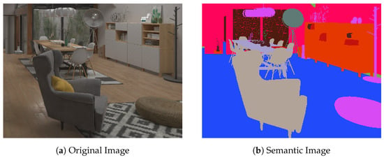
Figure 2.
Semantic adhesion phenomenon.
To distinguish between different instances of the same class in the image, this paper considers the differences in spatial position, such as the significant discrepancies in the depth information between objects like the sofa and the chair in the example above. The method employed here is to identify distance discontinuities in the depth image and map them onto the semantic image to segment connected semantics.
3.1.1. Depth Image Mutation Area Detection
The goal of this section is to detect the positions of abrupt changes in distance in the depth image, i.e., locations at which the depth values of adjacent pixels vary significantly. This objective is similar to edge detection in ordinary images; therefore, this paper adopts an edge detection approach.
Current edge detection methods can be divided into two categories: those based on first-order derivatives and those based on second-order derivatives. Common operators based on the former include Roberts, Prewitt, and Sobel. Meanwhile, the Laplacian operator [40] is frequently used for second-order derivatives. The first-order operator produces edge responses even on flat surfaces such as the ground and walls, and the response strengths at different positions on the same surface are inconsistent. This is due to the characteristics of the first-order operator and the depth image itself.
In light of the abovementioned factors, this paper uses the Laplacian operator to detect distance change regions in the depth image. In two-dimensional space, the Laplacian operator can be written as follows:
where and represent the second-order partial derivatives of the image function f in the x and y directions, respectively.
Since directly computing the second-order derivative is challenging, this paper uses a discrete convolution kernel K to approximate the Laplacian operator, as shown in the following equation:
The process of using the Laplacian operator to find distance change regions in the depth image is as follows:
- The depth image is convolved with the discrete convolution kernel K to obtain an approximation of the second-order derivative.
- The distance change positions are sought based on the convolution result.
- An appropriate threshold is applied to binarize the result.
Figure 3 depicts the distance change regions detected by the algorithm on the depth image. These regions reflect abrupt changes in the distance from the scene to the camera and can help segment semantic regions connected by different instances.
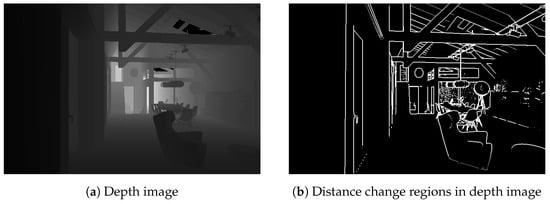
Figure 3.
Distance change detection in depth image.
3.1.2. Semantic Image Preprocessing
To eliminate the influence of semantic regions connected by different instances on the semantic image, this paper adopts the following processing steps:
- The method described in Section 3.1.1 is used to detect the positions of distance discontinuities in the depth image. This is based on the reasonable assumption that the distance from the camera to the same instance will remain relatively stable, while the distance from stuck regions of different instances will change.
- The semantic image is aligned with the depth image and the pixel values in the semantic image are set to correspond to the positions of distance discontinuities, which are shown in black, further segmenting the stuck regions.
- A preprocessed semantic image is created.
Figure 4 compares a semantic image before and after preprocessing. The preprocessed semantic image separates different instances with black lines, improving the discernibility of the semantic image.
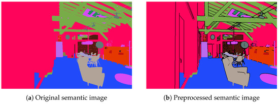
Figure 4.
Comparison between semantic images before and after preprocessing.
3.2. Semantic Vector-Based Coarse Matching Module
Due to the high computational complexity and time-consuming nature of the proposed semantic spatial structure-based fine matching module, it is infeasible to apply it to all historical frames. Therefore, in this paper, we utilize a hierarchical loop detection method, employing a coarse matching module to rapidly screen potential loop candidate frames from historical frames. Subsequently, the fine matching module is used to perform a more detailed similarity evaluation on the candidate frames in order to determine the existence of loops. This hierarchical loop detection method ensures accurate loop detection and improves the efficiency of our suggested method.
Figure 5 is a flowchart of the proposed semantic-vector-based coarse matching module, which includes the following steps:
- The semantic vector of the current frame is extracted as the basis for similarity evaluation.
- The similarity between historical frames and the current frame is evaluated based on semantic vectors.
- Non-maximum suppression is performed, and only the frame with the highest score among temporally adjacent frames is retained.

Figure 5.
Flowchart of semantic-vector-based coarse matching.
3.2.1. Semantic Vector Extraction
Semantic categories in semantic segmentation can be separated into dynamic semantic and static semantic classes based on whether they are in motion. Although the types and quantities of dynamic objects in the same scene may change frequently, the types and quantities of static classes remain relatively constant. Therefore, the types and quantities of static classes can provide preliminary screening for loop detection. When the types and quantities of static classes in two frames are similar, the probability that these two frames belong to the same scene is high, whereas, when there is a significant difference in the types and quantities of static classes between two frames, the likelihood that these two frames belong to the same scene is low. In light of this, a semantic vector extraction method is proposed in this paper.
The steps of the proposed method are as follows:
- For each frame, the semantic image is preprocessed using the method described in Section 3.1.1, as shown in Figure 6a.
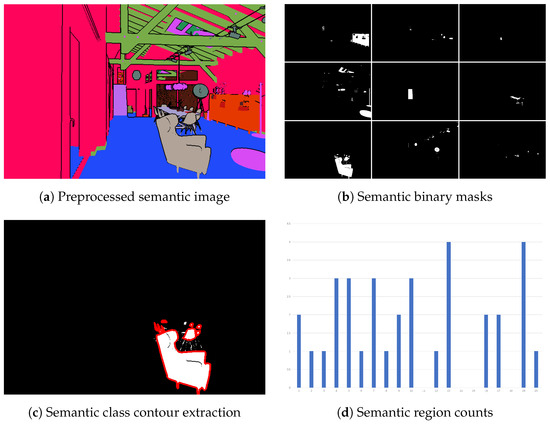 Figure 6. Semantic vector extraction.
 - For all static semantic classes, the semantics are extracted from the image through color lookup, forming a binary image. Figure 6b presents binary images of several major semantic classes. Notably, due to the lack of discrimination, walls and floors appear in almost all frames and are thus removed during this step.
- For each binary image, contour tracing is performed for extraction purposes. The contour extraction algorithm scans the image from the top-left corner, identifies the first white pixel, then moves along the boundary in a clockwise or counterclockwise direction, recording all the pixels passed until it returns to the starting point, thus obtaining a contour. This process is repeated until all regions have been traced. Figure 6c illustrates the contour extraction result for the chair semantic class.
- To form a vector that represents the types and quantities of objects in the current frame, the number of contours is used as an approximate value of the instance count. This vector is constructed by counting the number of occurrences of each semantic class and its corresponding contours that appear in the image. At this point, the length of the vector indicates the number of semantic classes in the environment, with the occurrence frequency of each semantic class in the current frame corresponding to the value at its position in the vector. If the contour area does not exceed a threshold , it is not considered. Figure 6d demonstrates an intuitive display of a semantic vector, where the horizontal axis represents semantic classes and the vertical axis represents the frequency of semantic occurrence.
3.2.2. Similarity Evaluation between Current Frame and Historical Frames
Although various measurement methods can be used to calculate the similarity between semantic vectors, such as the cosine similarity, Euclidean distance, Manhattan distance, and correlation coefficient, due to the significant differences in the value ranges of various semantics in this paper, using Manhattan and Euclidean distances to measure similarity is not appropriate. Considering the long-term operation of the SLAM system, which requires matching the current frame with a large number of historical frames, high demands are placed on computational efficiency and parallelism. Therefore, we do not adopt correlation coefficient methods in this paper, either. Consequently, cosine similarity is chosen to measure the similarity between semantic vectors.
Assuming there are two vectors and , their cosine similarity S can be calculated using the following formula:
Here, · denotes the dot product, represents the sum of element-wise multiplication of and , and and are the magnitudes of vectors and , respectively.
In addition to directly computing the cosine similarity between vectors, different weights can be assigned to different semantics. For example, items such as kitchenware and beds in indoor scenes possess higher robustness in semantic detection and can provide a better reflection of the current position information; thus, they can be assigned higher weights. Assuming the weights of different semantics are for a semantic vector , the weighted semantic vector can be obtained as follows:
where represents the new semantic vector obtained after incorporating weight information.
Once the methods for computing similarity between two vectors have been introduced, the similarity between the current frame and historical frames is calculated as follows:
- Since the similarity between adjacent frames is often high, but not meaningful for loop detection, a sliding window threshold is set in this paper. The loop detection algorithm does not evaluate the similarity between the current frame and the nearest frames.
- We calculate the similarity between the current frame and historical frames.
- We select the top k frames with the highest similarity scores from , where the similarity score exceeds the threshold .
The resulting k frames are the loop candidate frames in this paper. In addition to accelerating using matrix operations, fuzzy retrieval tools such as the Faiss library can also be utilized. Although the accuracy of fuzzy retrieval methods may decrease, their efficiency is superior; they are capable of handling retrievals at the billion level within milliseconds, making them suitable for SLAM systems that require higher real-time performance but have less stringent accuracy requirements.
3.2.3. Non-Maximum Suppression of Candidate Frames
Since adjacent image frames often contain similar scene information, to avoid redundant loop detection in the same scene, non-maximum suppression is performed on the k loop candidate frames obtained in the previous step. The detailed steps of this process are as follows:
- We arrange the similarity scores of the k loop candidate frames in descending order.
- Starting from the loop candidate frame with the highest similarity score, we remove the other loop candidate frames that exist within a time window T. Loop candidates with lower similarity scores around the frame with the highest score (scored at 0.9) are also removed, and new contenders are added to ensure an adequate number of candidates.
- The above steps are repeated until all loop candidate frames have been screened.
3.3. Fine Matching Module Based on Semantic Spatial Structure
After the coarse filtering of historical frames in Section 3.2, several candidate frames that may form loops with the current frame are obtained. However, relying solely on semantic vectors for similarity evaluation does not guarantee sufficient accuracy. For instance, different bedrooms or living rooms may have high semantic vector similarities. To address this issue, this paper introduces spatial structural information as a stronger constraint to further filter candidate frames.
The specific implementation steps of the proposed method are as follows:
- We extract the centroid positions of each contour area (i.e., each object) from the preprocessed semantic graph.
- We calculate the coordinates of the centroids in three-dimensional space.
- After that, we calculate the gravity direction based on SLAM frontend and IMU information.
- Next, we project the three-dimensional centroid positions along the gravity direction to reduce their dimensionality to two.
- Then, we utilize triangulation algorithms to extract the graph structure formed by the two-dimensional centroid positions.
- Finally, we use graph matching algorithms to calculate the graph structure similarity between the current frame and candidate frames, and multiply it by the vector similarity to obtain the final output.
3.3.1. Computation of Contour Centroids
This paper adopts the method introduced in Section 3.2.1 to extract all contours from the preprocessed semantic image and approximates each contour-surrounded region as an object. To fulfill the necessary processing steps required to obtain object position information, we must begin by determining the spatial coordinates of each object. Directly computing the point cloud corresponding to each object and finding its centroid is a more accurate approach, but is inefficient in this situation. Instead, a simpler and effective method is employed to calculate the centroid of each contour in the two-dimensional image and subsequently compute the centroid’s spatial coordinates as a representative of the object’s spatial position.
To compute the centroid of a contour, this paper utilizes the concept of moments in images. For a grayscale image where u and v are discrete variables, the equation can be transformed to
These are referred to as raw image moments. Using raw image moments, simple attributes such as the total grayscale sum and centroid can be computed as follows:
Figure 7 presents the centroid extraction results in actual operation. It can be observed that the majority of centroids effectively represent their corresponding regions.
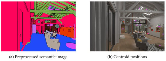
Figure 7.
Contour centroid computation result.
3.3.2. Computation of Centroid Spatial Coordinates
After obtaining the centroids of contours on the image, it is necessary to calculate their spatial positions in the camera coordinate system. The computation process varies depending on the sensor used. In this section, we employ a depth sensor to complete this calculation.
Upon aligning the depth image with the color image, the depth value at a pixel in the depth image represents the distance from the camera to the spatial point projected onto the color image at . Using the camera intrinsics and depth value, the spatial position of a point in the camera coordinate system can be identified.
According to the aligned images, this paper calculates the spatial coordinates of all contour centroids as an approximation of the objects’ positions in space. Figure 8 illustrates the spatial coordinates of centroids extracted in the previous section.
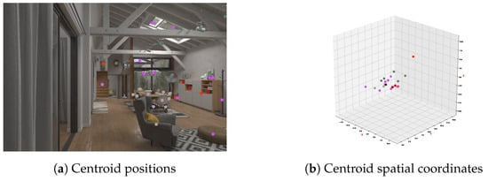
Figure 8.
Visualization of centroid spatial coordinates.
3.3.3. Computation of Gravity Direction
To determine the gravity direction of the current frame, this paper performs IMU initialization at the start of the SLAM system, determining the initial gravity direction, and subsequently identifies the gravity direction of the current frame based on the pose transformation matrices calculated by the SLAM frontend.
After IMU initialization, the initial gravity direction can be obtained. In this paper, we denote it as . Since the gravity direction in the camera coordinate system changes with the camera pose variations in subsequent frames, continuous tracking is required, necessitating the involvement of frontend pose information. Assuming the camera’s first frame pose change matrix calculated by the frontend after IMU initialization is , the new gravity direction can be computed as follows using the three-dimensional rigid body motion model:
As the frontend computes the pose change relative to the previous frame for each frame, only left multiplication of the previous frame’s gravity direction by the current frame’s rotation matrix is needed to identify the new gravity direction. Based on this principle, the gravity direction for the second frame can be computed as follows:
Continuing this recursively, the gravity direction for the nth frame is determined as follows:
At this point, the system can compute the gravity direction for all frames based on the initial gravity direction obtained from IMU initialization and the pose changes estimated by the frontend.
3.3.4. Projection of Centroids along Gravity Direction
In Section 3.3.2, we computed the spatial positions of all the centroids. Due to the high computational complexity of three-dimensional information, this section performs dimensionality reduction. The paper projects the point cloud along the gravity direction to compute the two-dimensional coordinates of each point on the ground plane as the result of dimensionality reduction.
3.3.5. Generation of Delaunay Triangulation Graph
A graph is a data structure used to represent objects and relationships using vertices and edges. In this paper, graph nodes represent objects, while the graph edges represent relative spatial relationships between objects, which allows us to describe the environmental information of a frame image using a graph structure.
The Delaunay triangulation algorithm possesses good connectivity and sparsity, and the generated graph structure is unique. Considering the above factors, this paper utilizes the Delaunay triangulation algorithm to generate a graph structure based on the two-dimensional point set. Delaunay triangulation is a method that partitions a set of points in a plane or space into triangles. It can be used to generate an undirected graph in which each point is a vertex and each edge connects two adjacent triangles.
After generating the graph structure for each frame image, it is necessary to evaluate the similarity of the graphs. For two given graphs, the method used to calculate similarity in this paper is as follows:
- The node similarity and edge similarity are calculated by comparing the similarity between nodes and edges in two graphs. In this case, node similarity is determined based on node semantics, where nodes with the same semantics have a similarity of 1, and nodes with different semantics have a similarity of 0. Edge similarity is calculated using the Gaussian affinity function. For two edges with lengths and , the edge similarity is calculated as follows:where is a constant, which is taken as in this paper.
- Next, the graph similarity matrix is established based on the node similarity matrix and edge similarity matrix.
- Next, optimal graph matching is achieved. The optimization objective function for graph matching is as follows:Here, is the similarity matrix calculated in the previous step, and is the column vectorized representation of the matching matrix. This paper employs the Reweighted Random Walks for Graph Matching (RRWM) algorithm [41] to compute the optimal matching between two graphs.
- The final similarity score between two graphs is calculated using the following formula:where s represents the similarity between two graph structures, ranging from 0 to 1, where 0 indicates complete dissimilarity and 1 indicates complete similarity. Additionally, represents the column vectorized representation of the optimal matching matrix, and and represent the number of matched nodes and edges, respectively.
The similarity results of vector matching and graph matching are multiplied to obtain the final loop detection score for two frame images. A high score indicates a strong probability of loop closure between two frame images.
4. Experimental Results and Analysis
4.1. Dataset Description
Based on the algorithm principle, the proposed method focuses on using the semantic information to improve the loop detection performance. This means that the method used to obtain the semantic information has no influence on the experimental conclusion. Therefore, to evaluate the performance of the proposed loop closure detection algorithm in indoor scenarios, we conducted experiments involving the Apartment scene from the uHumans2 dataset. The uHumans2 dataset provides rich information such as stereo camera images, depth images, 2D LiDAR, 2D semantic segmentation images, IMU data, ground truth odometry, etc. To simulate real-world scenarios, several semantic subclasses provided by the dataset were merged into multiple main categories.
4.2. Comparison of Algorithms and Important Parameter Settings
To evaluate the performance of the algorithm, it was compared with the Bag-of-Words model and a 2D image-based graph matching algorithm. The parameter settings for each algorithm are as follows:
- Semantic space structure-based loop closure detection algorithm: When performing the contour extraction, the minimum contour area was set as ; contours with an area smaller than this threshold were excluded from all subsequent computations. During semantic vector coarse matching, a non-maximum suppression window threshold of and a minimum similarity of were set.
- Bag-of-Words model: A properly sized tree with a depth of 5 and 10 branches was established as the dictionary of the Bag-of-Words model. During dictionary generation, all feature points of all images in the dataset were extracted, and their descriptors were then clustered layer by layer using the K-means++ algorithm. The final leaf nodes represented the words to which the features belong. The similarity between two images was then computed based on the constructed bag.
- ORB-SLAM3: This algorithm utilizes the vocabulary constructed by ORB-SLAM3 to build a bag of words and then computes the similarity between two images based on this constructed bag of words.
- Two-dimensional image-based graph matching algorithm: Spatial positions and projections in semantic space were not calculated. All other settings were the same as those of the proposed algorithm.
4.3. Robustness to Illumination Variation
To investigate the proposed method’s robustness to changes in illumination conditions, brightness variation and Gaussian noise were manually added to test images. Some examples are shown in Figure 9. The specific procedures for adding variations were as follows:
- Brightness variation: A brightness offset of was added to each pixel of the image, where was sampled from with intervals of 10 (except for 0). After adding the offset, pixel values exceeding the range of [0, 255] were clipped to 0 or 255.
- Gaussian noise: Gaussian noise with a mean of 0 and a standard deviation of was added to each of the RGB channels of each pixel, where was sampled from [5, 50] at intervals of five. Similarly, pixel values exceeding the range of [0, 255] were clipped.
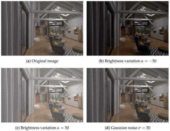
Figure 9.
Examples of illumination variation test cases.
The original images and the test images with brightness offsets or Gaussian noise were processed to extract semantics using the algorithms described in Section 3.1. In theory, the structured semantic features are superior to traditional point features and unstructured semantic features in loop detection. Therefore, the similarity was calculated using the Bag-of-Words model, the 2D image-based graph matching algorithm, ORB-SLAM3, and the proposed algorithm, and the results are shown in Figure 10. The x-axis represents the parameter values used for image alteration, the y-axis represents the similarity score, and the bar graphs of three colors represent the four algorithms.
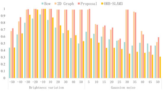
Figure 10.
Bag-of-Words model, 2D graph matching, ORB-SLAM3, and this article’s algorithm similarity evaluation result.
Firstly, the effect of brightness variation on the performance of the four algorithms was analyzed. Our results demonstrate that, when the brightness of the test image increased, both the proposed algorithm and the 2D image-based graph matching algorithm maintained high similarity scores due to the robustness of the semantic neural network in this scenario. However, the algorithm based on the Bag-of-Words model showed a significant decrease in performance. Furthermore, integrating ORB-SLAM3 into the analysis, we observe that it outperformed our trained Bag-of-Words model under these conditions but still fell short compared to the algorithms proposed in this study and the 2D image-based graph matching approach. Conversely, when the brightness of the test image decreased, the performance of the proposed algorithm was slightly better than that of the 2D image-based graph matching algorithm, while it exhibited a significant advantage over the algorithm based on the Bag-of-Words model, including ORB-SLAM3 and our trained Bag-of-Words model.
Next, the effect of adding noise on algorithm performance was analyzed. Compared with the algorithm based on the Bag-of-Words model, including ORB-SLAM3 and our trained Bag-of-Words model, the proposed algorithm achieved a superior performance in most cases, although the proposed algorithm’s scores fluctuated more due to the insufficient training of the neural network, causing the semantic segmentation results to be sensitive to noise interference. This issue can be addressed by further training the neural network. Compared with the 2D image-based graph matching algorithm, the proposed algorithm achieved an equal or slightly better performance.
In summary, the proposed algorithm exhibited superior robustness to illumination and noise, compared to traditional algorithms, and therefore was more conducive to loop closure detection.
4.4. Robustness to Viewpoint Change
To explore the robustness of the proposed loop closure detection method to changes in viewpoint, the living room scene from the Apartment dataset was selected as the validation object. This scene exhibited rich changes in viewpoint, as shown in Figure 11. Using Figure 11a as the reference frame, its similarity to other images was detected. Figure 12 shows some scenarios that are prone to false positives. Additionally, since adjacent frame images usually have high similarity, and the reference frame was the first frame in the dataset, similarity evaluation was not performed on the first 300 frames of the dataset.
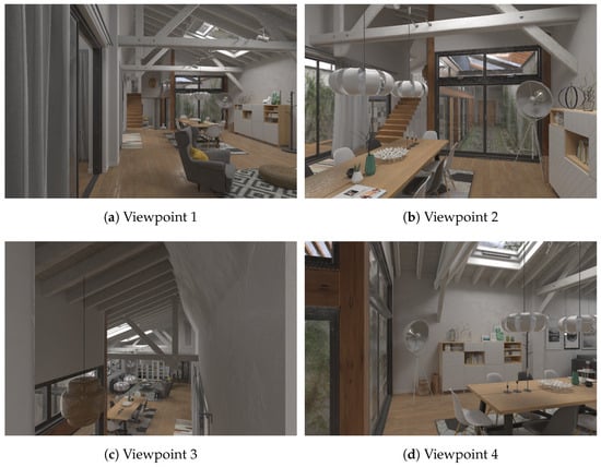
Figure 11.
Viewpoint change in living room scene.
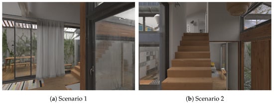
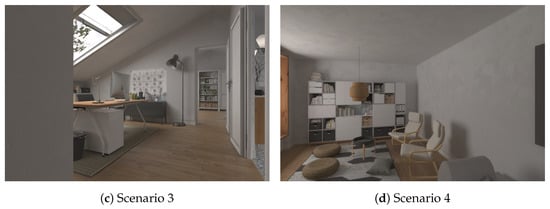
Figure 12.
Scenarios prone to false positives.
Figure 13 displays the similarity change curves for each frame using four different methods. The x-axis represents the frame number, while the y-axis represents the similarity score. The red dashed lines indicate the positions that correspond to three different shooting angles (Figure 11b–d); the black dashed lines indicate the positions that correspond to four scenarios that are prone to false positives (Figure 12a–d). A robust loop closure detection should exhibit high scores near the red dashed lines and significant differentiation from other positions, while scores near the black dashed lines should be as low as possible, with scores elsewhere remaining close to 0.
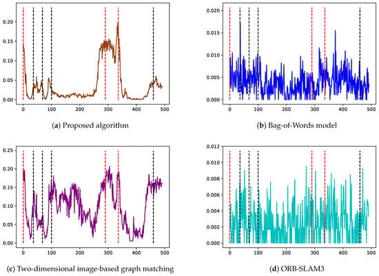
Figure 13.
Similarity change curves between the first frame and other frames.
Firstly, when we focus on the results of the Bag-of-Words model and ORB-SLAM3 (Figure 13b,d), these methods exhibit unstable performance when there are drastic changes in the shooting angle, with low scores observed in correctly matched regions and the highest scores in incorrectly matched regions. Secondly, for the 2D image-based method (Figure 13c), although there is an improvement in performance compared to the Bag-of-Words model, high scores are still observed in areas prone to false positives. Finally, when the method proposed in this paper is examined (Figure 13a), the correct closed-loop region achieves a significantly higher score, while the incorrect closed-loop region achieves a lower score.
To evaluate the performance of each algorithm, precision–recall curves were plotted, as shown in Figure 14. Precision–recall curves are a common method for evaluating loop closure detection performance, exhibiting the relationship between precision and recall under different threshold settings. Precision represents the proportion of all detected loops that are true positives, while recall represents the proportion of all true loops that are detected. When analyzing precision–recall curves, the focus is usually on two factors: the extent to which the curve shifts towards the upper-right corner and the recall value corresponding to 100% precision. The closer the curve is to the upper-right corner, the higher the precision at the same recall level, or the higher the recall at the same precision level. A higher recall value at 100% precision indicates that the algorithm can detect more true loops without false detections.
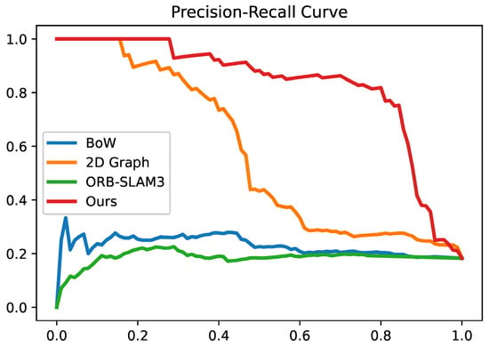
Figure 14.
Precision–recall curves.
Figure 14 shows that the proposed method achieves the best results, reaching a recall of nearly 30% at 100% precision and presenting the curve that is closest to the upper-right corner.
4.5. Ablation Experiments
We performed ablation experiments in order to assess the individual contributions of the semantic vector matching and the semantic space structure-based graph matching modules. Specifically, each module was removed from the fusion framework and the loop closure detection performance was evaluated independently.
Figure 15 presents the similarity change curves resulting from the ablation experiments. The first two subfigures correspond to the performance of the fusion framework after the removal of one module. The curves illustrate how the absence of each module affects the detection of correct loop closures and the occurrence of false positives.

Figure 15.
The similarity change curve between the first frame and other frames of each module and fusion result.
Initially, when removing the semantic space structure-based graph matching module (Figure 15a), the system exhibits a similar pattern. Though some correct loop closures may still be detected, the absence of spatial constraints results in a higher occurrence of false positives.
Conversely, when focusing on the semantic vector matching module (Figure 15b) removal, obviously, this component helps the system filter the space with similar semantics. Although some correct matches are detected, the false positive rate remains greater in spaces with similar spatial structures.
Lastly, when both modules are utilized (Figure 15c), the system’s performance significantly improves. Leveraging both semantic context and spatial constraints leads to more accurate loop closure detection, with reduced false-positive occurrences. This fusion of semantic vector matching and semantic space structure-based graph matching enhances the system’s robustness and effectiveness in loop closure detection.
These ablation experiments highlight the crucial roles played by both semantic vector matching and semantic space structure-based graph matching in the fusion framework, demonstrating their complementary contributions to robust loop closure detection.
4.6. Analysis and Discussions
4.6.1. Discussion of the Efficiency
In our current research, we conducted an in-depth investigation into methods of enhancing the efficiency of matching modules, particularly when working with vast amounts of data. The computational efficiency of our method based on ORB-SLAM3 is evaluated and shown in Table 1. As shown in the table, the time consumed by coarse matching is not significantly different from that consumed when using the ORB-SLAM3 algorithm. To achieve this, we introduced matrix operations to optimize the performance of the coarse matching module. Leveraging the parallel processing capabilities and computational efficiency of matrix operations, we successfully accelerated the speed of the module, accelerating the entire processing workflow.

Table 1.
The time consumed by our proposed algorithm and by ORB-SLAM3.
However, despite the significant boost in the efficiency of the coarse matching module, the fine matching module still requires frame-by-frame calculations to determine the matching degree between frames. Although this approach ensures accurate matching, it inevitably reduces the operational speed. Thus, we devised an innovative strategy in order to strike a balance between accuracy and efficiency.
The fine matching works specifically for the frames filtered via coarse matching. We utilize the coarse matching module to perform an initial screening of a large number of frames and identify a small subset of potential loopback candidate frames. This step significantly reduces the number of frames that require fine matching, reducing the computational burden. In the uHumans2 dataset used in our evaluation, for example, approximately 10 out of every 500 frames are filtered via coarse matching. Subsequently, we perform fine matching on these candidate frames using a frame-by-frame calculation method. This approach maintains high loop detection accuracy while improving overall efficiency by reducing the amount of computation required.
By adopting this strategy, our algorithm not only achieves real-time performance but also maintains a high level of accuracy in loop detection. This both enhances the responsiveness of our system and improves its reliability and stability when working with large-scale datasets. In the future, we will continue to investigate ways of optimizing our algorithms, further enhancing the performance and practicality of our system.
4.6.2. Discussion of the Lighting Condition Variation
The proposed structured semantic feature not only possesses the ability to compare semantic information with the traditional feature points, but also avoids issues associated with insufficient accuracy caused by spatial structures. We have demonstrated that our proposed method outperforms semantic feature and feature points to solve the problem of illumination change. It uses semantic information to obtain illumination-invariant features and uses spatial structure constraints to address the inaccuracy caused by semantic regions. In contrast, in experiments involving changes in lighting conditions, we used a roughly trained neural network to obtain semantic information. However, because the network had not been trained to a sufficient level, it was not sufficiently robust in the face of strong changes in light and, as such, our scheme did not exhibit such noticeable superiority in this case. By using semantic information, our method can more easily adapt to various lighting changes, including the local brightness variation of the same scene. Under ideal conditions, a fully trained network should be able to achieve better semantic segmentation results in the case of global light changes, local light changes, or picture noise, making our method more robust than traditional methods.
5. Conclusions
The loop closure detection algorithm proposed in this paper effectively addresses the issue of non-robust loop closure detection in scenarios in which there are significant changes in illumination and viewpoint by adding semantic and spatial structure information as constraints. Furthermore, our results indicate that the proposed method is more accurate and robust than traditional loop detection algorithms. This suggests that the proposed method can adapt to a wider range of complex scenarios, providing a potential solution to the challenges faced in loop detection tasks.
Author Contributions
Conceptualization, X.C. and L.J.; methodology, X.C. and Y.Z.; software, Y.Z., M.K. and J.W.; writing—original draft, Y.Z. and J.J.; writing—review and editing, Y.Z., M.K., J.W. and L.D. All authors have read and agreed to the published version of the manuscript.
Funding
This work was supported, in part, by the National Natural Science Foundation of China under Grant 62006178 and the Fundamental Research Funds for the Central Universities XJSJ23082.
Data Availability Statement
The uHumans2 datasets utilized in this study are publicly available for research purposes. The uHumans2 dataset can be accessed and downloaded from the Massachusetts Institute of Technology’s website at [https://web.mit.edu/sparklab/datasets/uHumans2/, accessed on 20 March 2024].
Conflicts of Interest
The authors declare no conflicts of interest.
Abbreviations
The following abbreviations are used in this manuscript:
| SLAM | Simultaneous Localization and Mapping. |
| LCD | Loop Closure Detection. |
| VPR | Visual Place Recognition. |
| BOW | Bag of Words. |
| ANN | Approximate Nearest Neighbors. |
| CNN | Convolutional Neural Networks. |
References
- Zhang, X.; Wang, L.; Su, Y. Visual place recognition: A survey from deep learning perspective. Pattern Recognit. 2021, 113, 107760. [Google Scholar] [CrossRef]
- Zheng, X.; Chen, X.; Lu, X.; Sun, B. Unsupervised Change Detection by Cross-Resolution Difference Learning. IEEE Trans. Geosci. Remote Sens. 2022, 60, 1–16. [Google Scholar] [CrossRef]
- Lowry, S.; Sünderhauf, N.; Newman, P.; Leonard, J.J.; Cox, D.; Corke, P.; Milford, M.J. Visual place recognition: A survey. IEEE Trans. Robot. 2015, 32, 1–19. [Google Scholar] [CrossRef]
- Lowe, D.G. Distinctive image features from scale-invariant keypoints. Int. J. Comput. Vis. 2004, 60, 91–110. [Google Scholar] [CrossRef]
- Bay, H.; Ess, A.; Tuytelaars, T.; Van Gool, L. Speeded-up robust features (SURF). Comput. Vis. Image Underst. 2008, 110, 346–359. [Google Scholar] [CrossRef]
- Dalal, N.; Triggs, B. Histograms of oriented gradients for human detection. In Proceedings of the 2005 IEEE Computer Society Conference on Computer Vision and Pattern Recognition (CVPR’05), IEEE, San Diego, CA, USA, 20–25 June 2005; Volume 1, pp. 886–893. [Google Scholar]
- Mur-Artal, R.; Montiel, J.M.M.; Tardos, J.D. ORB-SLAM: A versatile and accurate monocular SLAM system. IEEE Trans. Robot. 2015, 31, 1147–1163. [Google Scholar] [CrossRef]
- Mur-Artal, R.; Tardós, J.D. Orb-slam2: An open-source slam system for monocular, stereo, and rgb-d cameras. IEEE Trans. Robot. 2017, 33, 1255–1262. [Google Scholar] [CrossRef]
- Campos, C.; Elvira, R.; Rodríguez, J.J.G.; Montiel, J.M.; Tardós, J.D. Orb-slam3: An accurate open-source library for visual, visual–inertial, and multimap slam. IEEE Trans. Robot. 2021, 37, 1874–1890. [Google Scholar] [CrossRef]
- Qin, T.; Li, P.; Shen, S. Vins-mono: A robust and versatile monocular visual-inertial state estimator. IEEE Trans. Robot. 2018, 34, 1004–1020. [Google Scholar] [CrossRef]
- Arandjelovic, R.; Gronat, P.; Torii, A.; Pajdla, T.; Sivic, J. NetVLAD: CNN architecture for weakly supervised place recognition. In Proceedings of the IEEE Conference on Computer Vision and Pattern Recognition, Las Vegas, NV, USA, 27–30 June 2016; pp. 5297–5307. [Google Scholar]
- Nister, D.; Stewenius, H. Scalable recognition with a vocabulary tree. In Proceedings of the 2006 IEEE Computer Society Conference on Computer Vision and Pattern Recognition (CVPR’06), New York, NY, USA, 17–22 June 2006; Volume 2, pp. 2161–2168. [Google Scholar]
- Gálvez-López, D.; Tardos, J.D. Bags of binary words for fast place recognition in image sequences. IEEE Trans. Robot. 2012, 28, 1188–1197. [Google Scholar] [CrossRef]
- Cummins, M.; Newman, P. FAB-MAP: Probabilistic localization and mapping in the space of appearance. Int. J. Robot. Res. 2008, 27, 647–665. [Google Scholar] [CrossRef]
- Lepetit, V.; Lagger, P.; Fua, P. Randomized trees for real-time keypoint recognition. In Proceedings of the 2005 IEEE Computer Society Conference on Computer Vision and Pattern Recognition (CVPR’05), IEEE, San Diego, CA, USA, 20–25 June 2005; Volume 2, pp. 775–781. [Google Scholar]
- Newcombe, R.A.; Izadi, S.; Hilliges, O.; Molyneaux, D.; Kim, D.; Davison, A.J.; Kohi, P.; Shotton, J.; Hodges, S.; Fitzgibbon, A. Kinectfusion: Real-time dense surface mapping and tracking. In Proceedings of the 2011 10th IEEE International Symposium on Mixed and Augmented Reality, IEEE, Basel, Switzerland, 26–29 October 2011; pp. 127–136. [Google Scholar]
- Whelan, T.; Salas-Moreno, R.F.; Glocker, B.; Davison, A.J.; Leutenegger, S. ElasticFusion: Real-time dense SLAM and light source estimation. Int. J. Robot. Res. 2016, 35, 1697–1716. [Google Scholar] [CrossRef]
- Klein, G.; Murray, D. Parallel tracking and mapping for small AR workspaces. In Proceedings of the 2007 6th IEEE and ACM International Symposium on Mixed and Augmented Reality, IEEE, Nara, Japan, 13–16 November 2007; pp. 225–234. [Google Scholar]
- Glocker, B.; Shotton, J.; Criminisi, A.; Izadi, S. Real-time RGB-D camera relocalization via randomized ferns for keyframe encoding. IEEE Trans. Vis. Comput. Graph. 2014, 21, 571–583. [Google Scholar] [CrossRef]
- Milford, M.J.; Wyeth, G.F. SeqSLAM: Visual route-based navigation for sunny summer days and stormy winter nights. In Proceedings of the 2012 IEEE International Conference on Robotics and Automation, IEEE, Saint Paul, MN, USA, 14–18 May 2012; pp. 1643–1649. [Google Scholar]
- Siam, S.M.; Zhang, H. Fast-SeqSLAM: A fast appearance based place recognition algorithm. In Proceedings of the 2017 IEEE International Conference on Robotics and Automation (ICRA), IEEE, Singapore, 29 May–3 June 2017; pp. 5702–5708. [Google Scholar]
- Indyk, P.; Motwani, R. Approximate nearest neighbors: Towards removing the curse of dimensionality. In Proceedings of the Thirtieth Annual ACM Symposium on Theory of Computing, Dallas, TX, USA, 24–26 May 1998; pp. 604–613. [Google Scholar]
- LeCun, Y.; Bottou, L.; Bengio, Y.; Haffner, P. Gradient-based learning applied to document recognition. Proc. IEEE 1998, 86, 2278–2324. [Google Scholar] [CrossRef]
- Lopez-Antequera, M.; Gomez-Ojeda, R.; Petkov, N.; Gonzalez-Jimenez, J. Appearance-invariant place recognition by discriminatively training a convolutional neural network. Pattern Recognit. Lett. 2017, 92, 89–95. [Google Scholar] [CrossRef]
- Sünderhauf, N.; Shirazi, S.; Jacobson, A.; Dayoub, F.; Pepperell, E.; Upcroft, B.; Milford, M. Place recognition with convent landmarks: Viewpoint-robust, condition-robust, training-free. In Robotics: Science and Systems XI; 2015; pp. 1–10. Available online: https://www.roboticsproceedings.org/rss11/p22.pdf (accessed on 9 May 2024).
- Zitnick, C.L.; Dollár, P. Edge boxes: Locating object proposals from edges. In Proceedings of the Computer Vision–ECCV 2014: 13th European Conference, Zurich, Switzerland, 6–12 September 2014; Proceedings, Part V 13. Springer: Berlin/Heidelberg, Germany, 2014; pp. 391–405. [Google Scholar]
- Krizhevsky, A.; Sutskever, I.; Hinton, G.E. Imagenet classification with deep convolutional neural networks. Adv. Neural Inf. Process. Syst. 2012, 25. Available online: https://proceedings.neurips.cc/paper_files/paper/2012/file/c399862d3b9d6b76c8436e924a68c45b-Paper.pdf (accessed on 9 May 2024). [CrossRef]
- Hausler, S.; Garg, S.; Xu, M.; Milford, M.; Fischer, T. Patch-netvlad: Multi-scale fusion of locally-global descriptors for place recognition. In Proceedings of the IEEE/CVF Conference on Computer Vision and Pattern Recognition, Nashville, TN, USA, 20–25 June 2021; pp. 14141–14152. [Google Scholar]
- Zheng, X.; Sun, H.; Lu, X.; Xie, W. Rotation-Invariant Attention Network for Hyperspectral Image Classification. IEEE Trans. Image Process. 2022, 31, 4251–4265. [Google Scholar] [CrossRef]
- Zheng, X.; Yuan, Y.; Lu, X. A Deep Scene Representation for Aerial Scene Classification. IEEE Trans. Geosci. Remote Sens. 2019, 57, 4799–4809. [Google Scholar] [CrossRef]
- Zheng, X.; Gong, T.; Li, X.; Lu, X. Generalized Scene Classification From Small-Scale Datasets with Multitask Learning. IEEE Trans. Geosci. Remote Sens. 2022, 60, 1–11. [Google Scholar] [CrossRef]
- Zheng, X.; Cui, H.; Xu, C.; Lu, X. Dual Teacher: A Semisupervised Cotraining Framework for Cross-Domain Ship Detection. IEEE Trans. Geosci. Remote Sens. 2023, 61, 1–12. [Google Scholar] [CrossRef]
- Zheng, X.; Cui, H.; Lu, X. Multiple Source Domain Adaptation for Multiple Object Tracking in Satellite Video. IEEE Trans. Geosci. Remote Sens. 2023, 61, 1–11. [Google Scholar] [CrossRef]
- Zheng, X.; Chen, X.; Lu, X. Visible-Infrared Person Re-Identification via Partially Interactive Collaboration. IEEE Trans. Image Process. 2022, 31, 6951–6963. [Google Scholar] [CrossRef] [PubMed]
- Cascianelli, S.; Costante, G.; Bellocchio, E.; Valigi, P.; Fravolini, M.L.; Ciarfuglia, T.A. Robust visual semi-semantic loop closure detection by a covisibility graph and CNN features. Robot. Auton. Syst. 2017, 92, 53–65. [Google Scholar] [CrossRef]
- Zheng, X.; Wang, B.; Du, X.; Lu, X. Mutual Attention Inception Network for Remote Sensing Visual Question Answering. IEEE Trans. Geosci. Remote Sens. 2022, 60, 1–14. [Google Scholar] [CrossRef]
- Garg, S.; Suenderhauf, N.; Milford, M. Lost? appearance-invariant place recognition for opposite viewpoints using visual semantics. arXiv 2018, arXiv:1804.05526. [Google Scholar]
- Lin, G.; Milan, A.; Shen, C.; Reid, I. Refinenet: Multi-path refinement networks for high-resolution semantic segmentation. In Proceedings of the IEEE Conference on Computer Vision and Pattern Recognition, Honolulu, HI, USA, 21–26 July 2017; pp. 1925–1934. [Google Scholar]
- Garg, S.; Suenderhauf, N.; Milford, M. Semantic–geometric visual place recognition: A new perspective for reconciling opposing views. Int. J. Robot. Res. 2022, 41, 573–598. [Google Scholar] [CrossRef]
- Marr, D.; Hildreth, E. Theory of edge detection. Proc. R. Soc. Lond. Ser. B. Biol. Sci. 1980, 207, 187–217. [Google Scholar]
- Cho, M.; Lee, J.; Lee, K.M. Reweighted random walks for graph matching. In Proceedings of the Computer Vision–ECCV 2010: 11th European Conference on Computer Vision, Heraklion, Crete, Greece, 5–11 September 2010; Proceedings, Part V 11. Springer: Berlin/Heidelberg, Germany, 2010; pp. 492–505. [Google Scholar]
Disclaimer/Publisher’s Note: The statements, opinions and data contained in all publications are solely those of the individual author(s) and contributor(s) and not of MDPI and/or the editor(s). MDPI and/or the editor(s) disclaim responsibility for any injury to people or property resulting from any ideas, methods, instructions or products referred to in the content. |
© 2024 by the authors. Licensee MDPI, Basel, Switzerland. This article is an open access article distributed under the terms and conditions of the Creative Commons Attribution (CC BY) license (https://creativecommons.org/licenses/by/4.0/).