Memory Augmentation and Non-Local Spectral Attention for Hyperspectral Denoising

Abstract

In this paper, a novel hyperspectral denoising method is proposed, aiming at restoring clean images from images disturbed by complex noise. Previous denoising methods have mostly focused on exploring the spatial and spectral correlations of hyperspectral data. The performances of these methods are often limited by the effective information of the neighboring bands of the image patches in the spectral dimension, as the neighboring bands often suffer from similar noise interference. On the contrary, this study designed a cross-band non-local attention module with the aim of finding the optimal similar band for the input band. To avoid being limited to neighboring bands, this study also set up a memory library that can remember the detailed information of each input band during denoising training, fully learning the spectral information of the data. In addition, we use dense connected module to extract multi-scale spatial information from images separately. The proposed network is validated on both synthetic and real data. Compared with other recent hyperspectral denoising methods, the proposed method not only demonstrates good performance but also achieves better generalization.

1. Introduction

Unlike natural images and traditional grayscale images, hyperspectral images (HSIs) collected through hyperspectral sensors contain over a hundred spectral bands for the same scene [1,2,3]. Benefiting from the richness of spectral information, HSIs play a crucial role in earth observation, such as target detection [4], mineral exploration [5], image classification [6], and more. However, due to the complexity and uncertainty of imaging, HSIs inevitably suffer from noise interference, including Gaussian noise, striping noise, and mixed noise [7]. The presence of image noise reduces image quality and affects the interpretation of target information, which greatly hinders the application of hyperspectral images. Therefore, hyperspectral denoising algorithms have emerged to enhance image quality as much as possible.

In recent years, a large number of denoising algorithms have been proposed for HSIs disturbed by noises. According to the solution method, these can be divided into three categories, which are filtering-based denoising methods, optimization-based denoising methods, and deep learning-based denoising methods [7,8,9].

1.1. Filtering-Based Methods

Filtering-based methods comprise spatial filtering denoising approaches and transform domain-denoising methods [10]. Specifically, spatial filtering methods employ various operators in the spatial domain to eliminate image noise [11,12,13,14,15]. In [13], a multidimensional Wiener filtering was designed for hyperspectral denoising, treating an HSI as a third-order tensor and utilizing filtering along different directions to remove noise in different dimensions of the image. A Gabor filter was employed to detect stripe patterns in each band [14]. Simultaneously, transform-based denoising methods utilize various projection transformations to recover a clean image from the contaminated image, including Fourier transform [16], Wavelet transform [15], and Principal Component Analysis (PCA) [17], among others. To be specific, the proposed approach HSSNR [15] uses Wavelet transform to learn the signal variation in the spectral and spatial dimensions of hyperspectral data. PCA was introduced in [17], in which a 2-D bivariate wavelet threshold and 1-D dual-tree complex wavelet transform method are introduced to improve image quality. Additionally, the well-known BM4D [18] implements the group collaborative filtering paradigm, in which similar patches are stacked in a high-dimensional array, and the image quality is improved via joint filtering in the transform domain.

1.2. Optimization-Based Methods

Recently, optimization-based denoising methods have been greatly developed, which use a variety of optimization methods to improve the stability and effectiveness of algorithms, including low-rank [19], sparse representation [20,21] and self-similarity [22,23] methods. Specifically, due to the limited distribution of spatial ground objects and the correlation of multiple adjacent spectra, low-rank attributes widely exist in the spatial and spectral dimensions of hyperspectral images. So far, a large number of methods based on low-rank constraints and subspace learning have been applied to HSI denoising [24]. Meanwhile, a KBR-based tensor sparsity measure was proposed in [25], where a tensor is sparsely represented using Tucker decomposition and CP decomposition. In [26], a strategy utilizing low-rank matrix recovery (LRMR) was proposed, which focuses on learning the features of stripe noise. Considering that each band in an HSI may be affected by different levels of noise interference, an adaptive iterative factor selection strategy combining low-rank matrix factorization was proposed (NAILRMA) in [27]. Its main innovation was to optimize and solve the problem of noise inconsistency in different bands. In addition, due to the continuity and universality of the distribution of hyperspectral objects, self-similarity is an inherent property of hyperspectral images, which has been widely used in many popular denoising methods. At present, the development trend of spectral denoising methods is to combine the spatial and spectral similarity of images to improve the quality of images [28,29]. In [30], the authors proposed a low-rank restoration method that combines spatial and spectral information for image denoising, which simultaneously embeds the TV regularization, nuclear norm, and $L_1$ norm (LRTV). TV regularization is used to maintain the spatial structural information of the image, while the nuclear norm is used to learn the low-rank attributes of the spectrum. This method has a good effect on removing multiple types of noise. Unfortunately, optimization-based methods usually require hand-crafted priors and iterative solutions, which hinders the performance of HSI denoising to a certain extent.

1.3. Deep Learning-Based Methods

Due to the automatic learning of features, deep learning-based denoising methods have attracted increasing attention [31]. As is well known, there is the strong correlation in the spatial and spectral dimensions of HSIs; hence, various methods have been dedicated to learning the spatial and spectral information. For instance, Chang et al. proposed a denoising method based on convolutional neural networks (HSIDeNet) [32] that aggregates the multi-scale contextual information of images through dilated convolution and multi-channel filters. Ref. [33] proposed a spectrally enhanced rectangular transformer to explore the non-local similarity and the low-rank properties of HSIs (SERT). A model with noise intensity estimation (Partial-DNet) was designed for HSI blind denoising in [34]. The noise intensity of each frequency band is estimated, and the channel attention mechanism is introduced, which is subsequently fused with the observed image to generate a feature map. In [35], a recursive neural network (QRNN3D) was used for denoising that can simultaneously explore the spatial spectral correlation and global correlation of images. Dong et al. proposed a separable 3-D denoising method that can significantly reduce computational costs [36]. Yuan et al. proposed a single-band deep convolutional neural network denoising method (HSI-DCNN) that takes into account the spatial and spectral information of HSIs [37]. HSI-DCNN uses a single band and its adjacent bands as inputs to the network, while utilizing multi-scale features to improve feature-expression capabilities. In addition, Maffei et al. proposed an image denoising method (HSI-SDeCNN) based on a single-model convolutional neural network [38]. HSI-SDeCNN uses noise level mapping to balance denoising results, and the raw data detail information. Unfortunately, these methods only consider the relationships among adjacent bands and fail to capture the inter-relationships on a global scale in the spectral dimension. The above methods all fail to consider the non-local and global similarity of hyperspectral images in the spectral dimension.

To alleviate the above problems, this paper proposes a novel hyperspectral denoising method based on non-local memory-augmented spectral attention. Specifically, the proposed network consists of two stages. In the first stage, a Dense Connected Module (DCM) is used to extract local spatial information from hyperspectral images. In addition, this method utilizes the multi-layer spatial information of HSIs as much as possible by inputting three different scales. The second stage of the network mainly explores spectral similarity information in the HSIs, which includes two modules: a non-local spectral attention and a global spectral memory-augmented module (MAN). Among them, the non-local attention module aims to extract useful information from adjacent band features to supplement the current band information and remove noise. In this module, similar band features in the neighborhood are queried based on the current band features, which can explore non-local structural information in the spectral dimension. However, this approach ignores the global structural relationship of the spectrum. To address this issue, this study designed a global memory-augmented attention module. This module sets up a global memory library to remember the information of all bands in the data and uses the features of the current band to directly query all useful information in the memory library for restoring the current band. Subsequently, combining the outputs of the two spectral attention modules and processing them further through convolutional layers before fusing them with the original features can help the model capture different spectral aspects of the input data and integrate them effectively. Finally, the upsampling module is used to fuse the information from three scales and output the denoising result. The denoising performance of our proposed method conducted on synthetic and real data demonstrates its superiority over state-of-the-art methods. In summary, the contributions of this study can be concluded as follows:

• Using the current band and its adjacent K bands as inputs to the network, the DCM is used to extract spatial information from the inputs, and it is applied on multi-scale spaces to fully learn the spatial structure of the image.
• The non-local memory-augmented spectral attention module is designed to learn the non-local and global correlations among data spectra at each scale.
• A series of ablation experiments were conducted, and the results were compared with those of existing methods on both synthetic and real data, which demonstrate the superiority of the proposed method.

The remainder of this paper is arranged as follows. Section 2 introduces the concepts related to hyperspectral denoising. The proposed network is described in detail in Section 3. The experimental results are discussed in Section 4. A summary of this paper is presented in Section 5.

2. Related Work

Due to the instability of sensors and the influence of the atmosphere, the collected HSIs often contain various types of noise. The purpose of the hyperspectral denoising task is to restore clean images X from noisy images Y, and the noise model can be expressed as follows:

$$Y=X+N$$

(1)

where Y represents a noisy HSI with the size of $H\times W\times B$, and B is the band number of the hyperspectral data. X is the clean image, and N denotes all random noise in the image. As previously studied [39], N may be the stripe noise, Gaussian noise, and the impulse noise, as well as various complex mixed noises.

To obtain clean images X, a large number of hyperspectral denoising methods have been proposed. Specifically, deep learning-based methods are widely used to learn the deep features of images. The mainstream idea of deep learning-based denoising methods is to explore the spatial and spectral information of the hyperspectral data, which can compensate for the information loss of the input spectral band and improve the denoising performance [40,41,42,43]. However, most of these methods are unable to fully learn the spectral structure of the data. In particular, when adjacent bands are affected by similar noise interference, the learned neighborhood band information cannot provide more effective information supplementation for the input band, resulting in a low denoising performance.

3. Proposed Method

Most of the existing denoising methods do not consider the non-local relationship among spectral bands. When facing complex noise, the performance of most methods is significantly reduced, affecting the performance of image quality improvement. To solve the above problems, this study also set up a memory library that can remember the detailed information of each input band during denoising training, fully learning the spectral information of the data. In addition, we use a dense connected module to extract multi-scale spatial information from images separately. This method can learn the non-local structural relationship between the space and spectrum to improve the denoising effect.

3.1. Overall Network Architecture

As shown in Figure 1, the network mainly includes two stages, which are spatial information extraction and non-local spectral information augmentation.

In the first stage of the network, a Dense Connected Module (DCM) is used to extract the spatial multi-scale features of the input current band and its adjacent K bands, aiming to fully utilize the spatial multi-scale information of the data in the denoising process. The second stage of the network consists of two modules: a non-local spectral attention module and a global spectral memory-augmented module. The non-local spectral module aims to extract useful spectral information from adjacent band features. In this module, the current band feature $F_b$ is used to query neighboring band features. The memory-augmented attention module utilizes a global memory library to remember useful information from adjacent bands in the training set and then uses the current band features to directly query the memory library for useful information when restoring the current band. Subsequently, convolving with a kernel size of 1 and fusing two spectral attention outputs $X_b$ and $Y_b$ with the current band feature can further improve the model’s ability to extract relevant information from the input data. Finally, the upsampling module is used to fuse the information from three scales and output the final denoising result.

3.2. Spatial Information Extaction Module

Due to the fact that traditional convolutional neural networks can capture the features of similar objects in different local regions using stacked convolutional layers to extract hierarchical features, we use a dense connected network [44] to extract local features, as shown in Figure 2. According to Figure 2, the output of the DCM module can be obtained as follows:

$$F_l=Relu(W_l\otimes fuse(F_{in},F_1,\dots F_{l-1})),l=1,\dots \mathrm{L}$$

(2)

where l denotes the layer of network, and the activation function Relu is used here. $W_l$ represents the convolutional kernel size, and $fuse$ (.) is a fusion operation. Then, the features $F_l$ extracted from each layer are fused as the final extracted features. The advantage is that multiple layers of local spatial feature representations can be obtained. The fusion operation can be obtained through a 1 × 1 convolution operation, which can be expressed as follows:

$${\mathrm{F}}_{\mathrm{DCM}}=W_{fuse}\otimes fuse(F_{in},F_1,\dots F_L)$$

(3)

where ${\mathrm{F}}_{\mathrm{DCM}}$ is the output of the spatial information extraction module. $W_{fuse}$ is the weight parameter during fusion.

3.3. Non-Local Memory-Augmented Attention Module

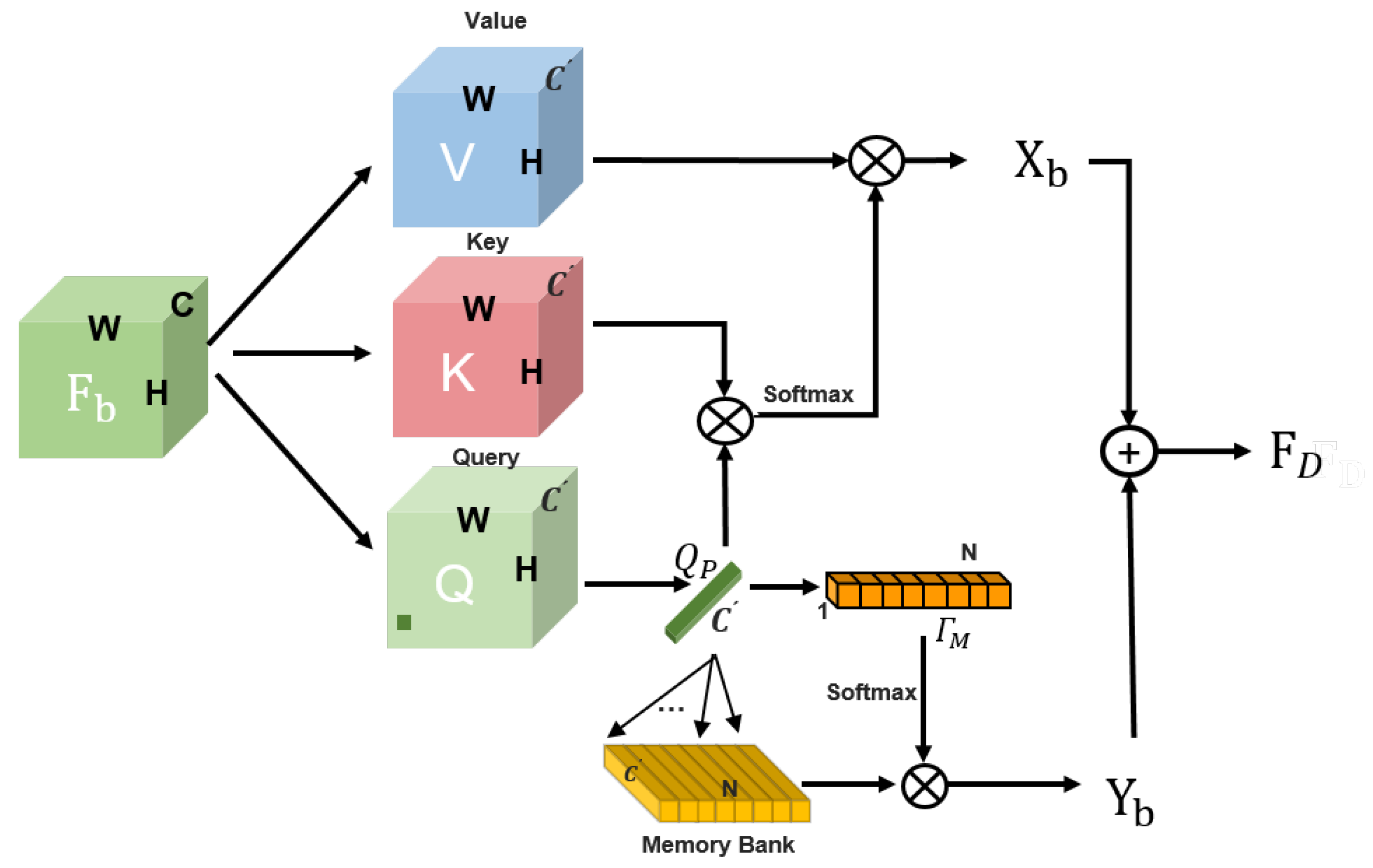
Given the current band $I\in R^{H\times W}$ of the image, its adjacent bands are $\left\{I_{b-\tau ,\cdots ,}{I}_{b+\tau }\right\}$, where H and W are the height and width of the HSI, and $T=2\tau +1$ represents the neighboring band span of the current band. In the first stage of our network, each band is passed through a DCM in the feature space to obtain a feature map $\left\{F_{b-\tau ,\cdots ,}{F}_{b+\tau }\right\}$. To model the non-local spectral correlation of the HSI, we designed a cross-band non-local spectral memory-augmented attention network (MAN), as shown in Figure 3.

The MAN consists of two parts, namely, the non-local spectral attention module and the global spectral memory-augmented attention module.

Firstly, the output feature $F_b\in R^{C^{\prime }\times H\times W}$ in the first stage of the current band is used as the query tensor, while the output feature $\{F_{b-\tau },\dots F_{b+\tau }\}$ of adjacent bands is used as the key tensor and value tensor, where C is the dimension of the feature map. In Figure 3, the tensors $Q\in R^{C^{\prime }\times H\times W}$, $K\in R^{C^{\prime }\times H\times W}$, and $V\in R^{C^{\prime }\times T\times H\times W}$ represent the query tensor, the key tensor, and the value tensor, respectively, where $C^{\prime }=C/2$. Generally, Q and K are directly matrixed into $\widehat{Q}\in R^{HW\times C\prime }$ and $\widehat{K}\in R^{C\prime \times HWT}$. The correlation matrix $\Gamma$ is then calculated as $\Gamma =\widehat{Q}\widehat{K}$.

The biggest drawback of this strategy is the introduction of large matrix operations, which imposes a heavy burden on computer memory. Therefore, to alleviate this phenomenon, we set the focus on the neighborhood of a single band, and at this point, the scale of $\Gamma$ is $HW\times HW,$ which can greatly reduce the computational cost. The goal of non-local spectral attention in hyperspectral denoising tasks is to query as many bands as possible in the spectral dimension that are most similar to the current band. However, if there is a significant difference in the spectral bands found, this not only leads to excessive network computation but also reduces the denoising performance.

To reduce matching errors in spectral bands, similar to [45], a Gaussian weight G was set here, which is multiplied by the correlation matrix $\Gamma$, and the center of the Gaussian map is located at the position of the query band. In short, the Gaussian map of each band in the first dimension of $\Gamma$ is different. Throughout the entire network learning process, the standard deviation of the Gaussian function is used as a learnable parameter to find the optimal denoising performance. The learnable Gaussian map can maintain a good balance between the non-local and local relationships in spectral dimensions. Ultimately, the output of the cross-band non-local attention module can be expressed as follows:

$$X_b=(\Gamma \otimes G)·V$$

(4)

where ⊗ is a Hadamard product.

However, due to the frequent approximation of noise interference between adjacent bands, the complementary information is limited. Therefore, we attempt to find the best non-local correlation band for the current band from a global perspective to better supplement spectral information for denoising. For this purpose, we set up a memory-augmented spectral attention network here. This module maintains a global memory $\mathbf{S}$, which is a learnable parameter in the network. Therefore, all non-local correlated bands of the current band are queried in the memory $\mathbf{S}$, which is ${\Gamma }_S=\widehat{Q}\mathbf{S}\in R^{HW\times N}$. The final output $Y_b$ can be obtained through the following steps:

$$Y_b=softmax\left({\Gamma }_S\right)·{\mathbf{S}}^T$$

(5)

And then, the output $X_b$ and $Y_b$ of the cross-band non-local spectral attention module and the memory-augmented module are fused through a 1 × 1 convolution and added as residuals to the input feature $F_b$ of the current band. Finally, the upsampling module is used to fuse information from three scales and output the final denoising result.

3.4. Implementation Details

Firstly, the three scale sizes are 32, 64, and 128. The first $\tau$ and last $\tau$ bands adjacent to the current band are taken as inputs for the network, where $K=2\tau$. Then, these cropped image patches are randomly flipped by 90 degrees, 180 degrees, and 270 degrees in the horizontal direction to enhance the diversity of the training data. Next, an Adam optimization algorithm was used to optimize the network. The initial learning rate was set to $2\times {10}^{-4}$, and the number of iterations was set to 200.

4. Experiments and Discussions

To demonstrate the effectiveness of the designed network, experiments were conducted on four datasets, including Washington DC (WDC) data, Pavia Center (PC) data, and Pavia University and Indian Pines data. Among them, WDC data and PC data were used as the basic data for synthesizing noise, and Pavia University and Indian Pines data were used as real-scene HSIs to further verify the practicality of all denoising methods. Due to the proposed method being an HSI denoising method based on spatial and spectral similarity constraints, five popular comparison methods were selected here, namely, LRMR [26], NAILRMA [27], LRTV [30], Partial-DNet [34], and SERT [33]. It is worth noting that LRMR, NAILRMA, and LRTV are all traditional optimization-based methods that improve the performances of algorithms by linearly characterizing the spatial–spectral structure of HSIs. In contrast, Partial-DNet and SERT learn the inter-relationships within HSIs through deep networks, and they have advantages in hyperspectral denoising tasks due to their ability to learn deep features of the data. This section demonstrates the effectiveness of the proposed method in exploring spatial and spectral structures by comparing the denoising results of six algorithms on different datasets.

To train the denoising network, the minimum residual MSE loss function is used here, which is mathematically expressed as follows:

$$L\mathrm{oss}=\frac{1}{2N}\sum _{i=1}^N{\left|\right|Net(y_i,k_i,\theta )-{\phi }_i\left|\right|}_2^2$$

(6)

where N denotes the training image pairs. ${\phi }_i=y_i-x_i$, and $x_i$, $y_i$, and $k_i$ denote the ith band of the clean image, the ith noisy band, and K bands in the neighborhood of the current band, respectively. $\theta$ is the network trainable parameters. This section also uses three widely used quantitative evaluation indicators to measure the denoising performance of the algorithms, namely, the PSNR, SSIM, and SAM. Specifically, the PSNR and SSIM compare the pixels of HSI images before and after denoising, while the SAM compares the spectral angular distance of images before and after denoising. To make the comparison of all algorithms more fair, sll experiments were conducted on the PyTorch platform using an NVIDIA RTX 3080 GPU.

4.1. The Synthetic Data Experiments and Discussions

The WDC contains hyperspectral data with a size of 1280 × 303 × 191. Images with a random sampling size of 1080 × 303 × 191 were used for training, while the rest were used for testing. The original size of the PC dataset was 1096 × 715 × 102, of which 1096 × 480 × 102 was used for training, and the rest was used for testing. When synthesizing data, similar to [46], four different levels of noise were added to the WDC and PC data to test the denosing methods’ ability for the following, different levels of noise:

(1) Case 1: In each band, zero-mean Gaussian noise with a variance of 0.1 is added;

(2) Case 2: In each band, zero-mean Gaussian noise with a variance range of 0.1~0.2 is added;

(3) Case 3: On the basis of Case 2, 20 bands are randomly selected and receive impulse noise with a variance of 0.2;

(4) Case 4: On the basis of Case 3, deadline noise is added with a width of 1–3 to 20 bands, with 10 bands selected from the bands with added impulse noise.

The quantitative results of all compared algorithms and the proposed method for HSI denoising conducted on four levels of noise data are shown in

Table 1. Results on the WDC Mall Data. Bold represents the optimal result.

Case		Case 1			Case 2			Case 3			Case 4
Dataset	Method	PSNR	SSIM	SAM	PSNR	SSIM	SAM	PSNR	SSIM	SAM	PSNR	SSIM	SAM
WDC Mall	Noisy	20.12	0.7881	17.6382	16.83	0.6634	24.2778	16.1	0.6285	26.4034	16.11	0.6277	26.4657
	LRMR	32.42	0.9783	4.9984	30.02	0.9638	6.2842	29.79	0.9626	6.2298	29.71	0.9622	6.3255
	NAILRMA	32.07	0.9779	5.2971	30.61	0.9686	5.9188	30.19	0.966	6.0014	30.04	0.9654	6.1164
	LRTV	33.04	0.9807	4.2104	31.1	0.9690	5.1222	30.8	0.9667	5.8929	30.76	0.9665	6.8520
	Partial-DNet	34.56	0.9870	3.4544	31.29	0.9752	5.4685	30.43	0.9705	5.9257	30.61	0.9718	5.8856
	SERT	33.23	0.9862	3.2852	31.04	0.9738	3.7545	30.16	0.9653	4.3179	30.44	0.9729	4.2128
	Ours	35.05	0.9886	2.0968	32.65	0.9809	2.7523	32.70	0.9794	2.9013	32.16	0.9791	2.8974

and

Table 2. Results on the Pavia Center Data. Bold represents the optimal result.

Case		Case 1			Case 2			Case 3			Case 4
Dataset	Method	PSNR	SSIM	SAM	PSNR	SSIM	SAM	PSNR	SSIM	SAM	PSNR	SSIM	SAM
Pavia Centre	Noisy	20.11	0.7761	18.688	16.96	0.6536	24.8008	15.34	0.5686	28.6074	15.41	0.5707	28.5094
	LRMR	31.74	0.9704	5.4259	29.13	0.9489	7.1564	28.4	0.9407	7.2550	28.2	0.9405	7.4484
	NAILRMA	32.99	0.9765	4.5047	30.5	0.9605	5.784	29.31	0.9508	6.0994	28.86	0.9492	6.5254
	LRTV	32.32	0.9712	4.9303	30.07	0.9517	7.8147	29.51	0.9392	9.8325	29.5	0.9373	11.3173
	Partial-DNet	34.48	0.9863	3.4566	31.87	0.9784	4.5559	30.15	0.9721	5.4706	30.38	0.9724	5.3533
	SERT	34.78	0.9869	2.5432	32.61	0.9797	2.7931	31.69	0.9934	2.9822	31.82	0.9737	3.9649
	Ours	35.16	0.9881	2.2259	33.14	0.9826	2.7808	32.41	0.9799	3.0055	32.22	0.9793	3.0561

. Among them, the best denoising results for each metric are displayed in bold. From Table 1 and Table 2, it can be seen that the proposed method is significantly superior to the LRMR, NAILRMA, and LRTV methods on the WDC dataset and the PC dataset. Because all three kinds of methods are based on low-rank matrices, they lose the spatial structure information of data during the denoising process.

In analyzing the denoising results of different types of noise data, it is evident that deep learning-based HSI denoising methods are generally superior to traditional machine learning-based methods. Deep learning-based denoising methods fully consider the spectral and spatial correlations of hyperspectral images. In comparing the Partial and SERT methods based on deep learning, it was found that the proposed method can achieve better results than the other methods in most of the three evaluation indicators. The above results indicate that the proposed method is beneficial in exploring the spatial–spectral relationship of HSIs. Its use of local memory-enhanced spectral attention techniques can fully learn the relationship between the spectral dimensions of data, thereby better restoring clean images. In addition, it can be summarized from Table 1 and Table 2 that as the types of noise become increasingly complex, the performances of all algorithms decrease, but the proposed method performs more stably when dealing with different levels of noise.

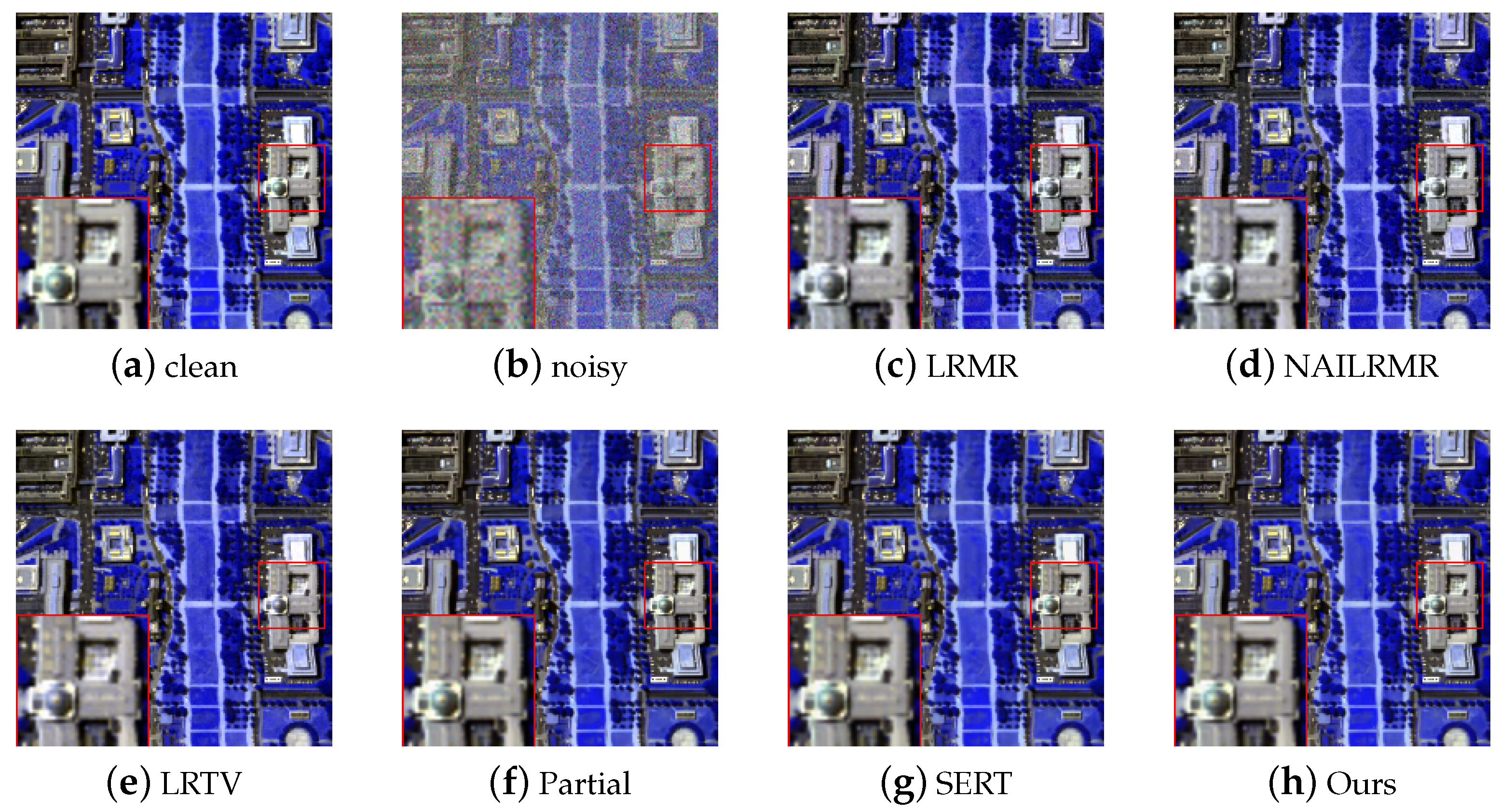
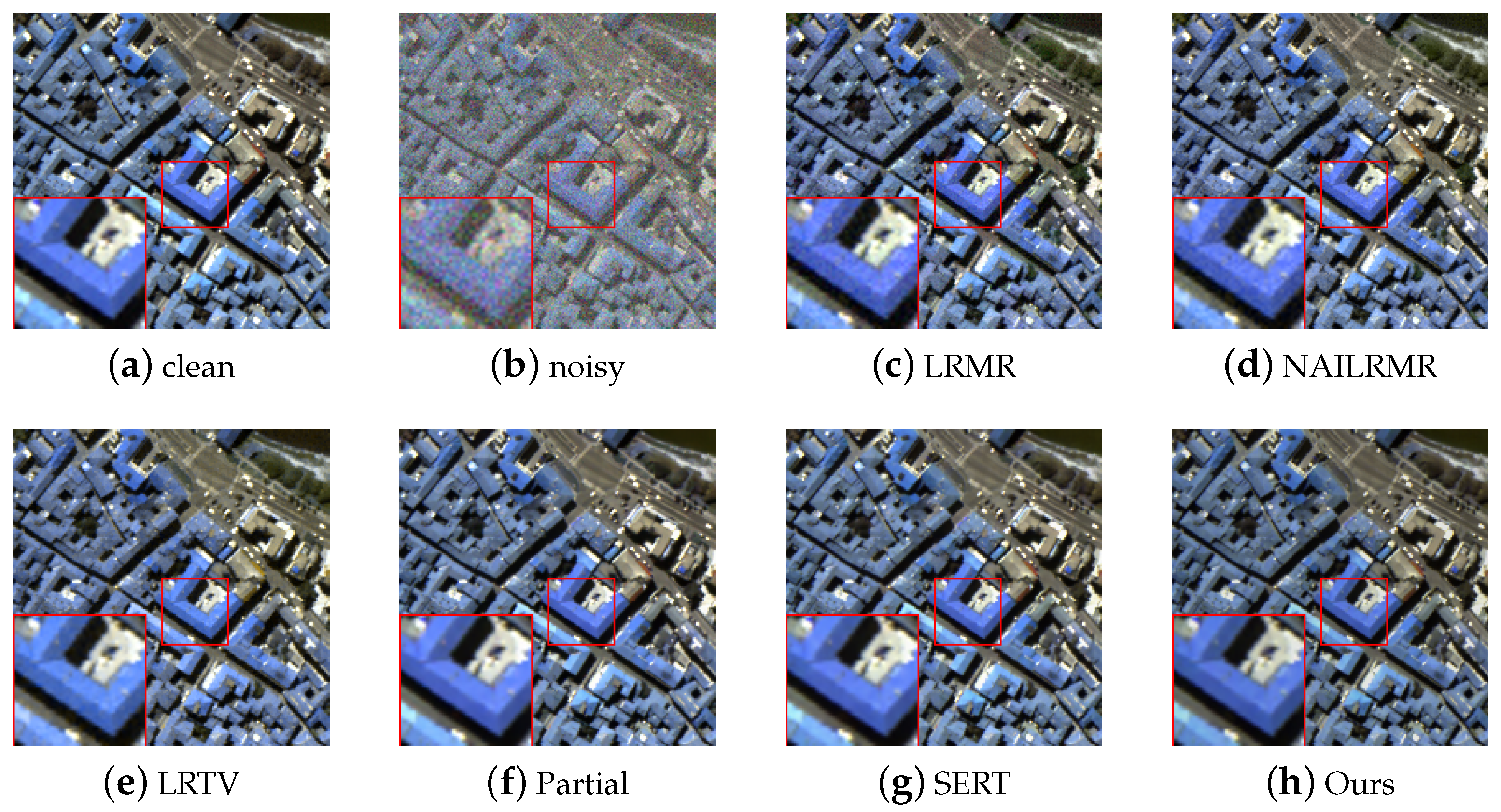
To comprehensively compare the denoising effects, the visualization results of denoising for Case 2 data are shown in Figure 4 and Figure 5. From Figure 4 and Figure 5, it can be seen that there is some residual noise in the denoising results of LRMR, NAILRMA, and LRTV. At the same time, Partial DNet and SERT have good denoising effects, but the denoised images still have some noise and incomplete structural information preservation, losing many details. In contrast, the proposed algorithm has better reconstruction results, especially in some detail and edge areas, which can be restored more clearly.

4.2. The Real Data Experiments and Discussions

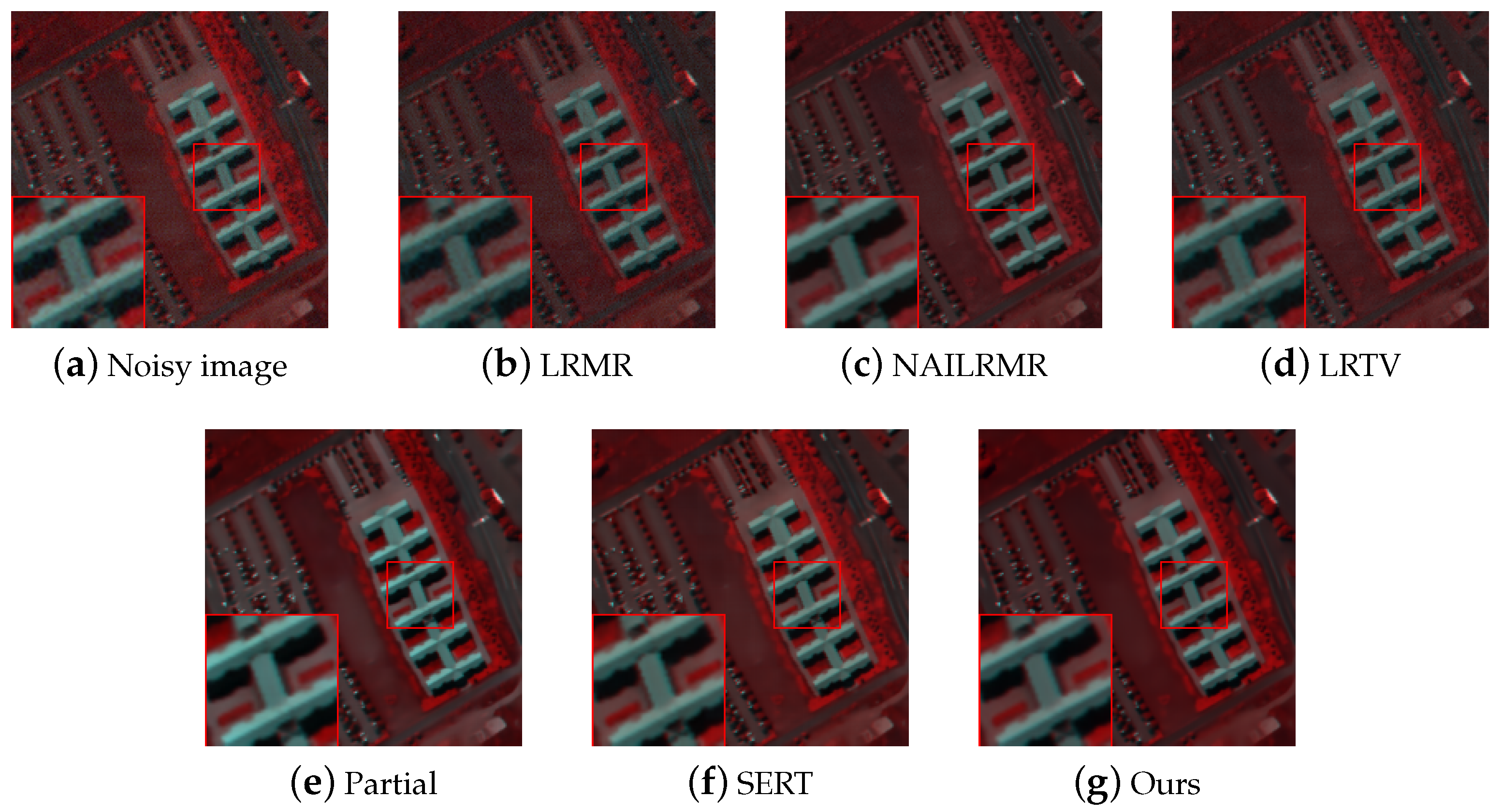
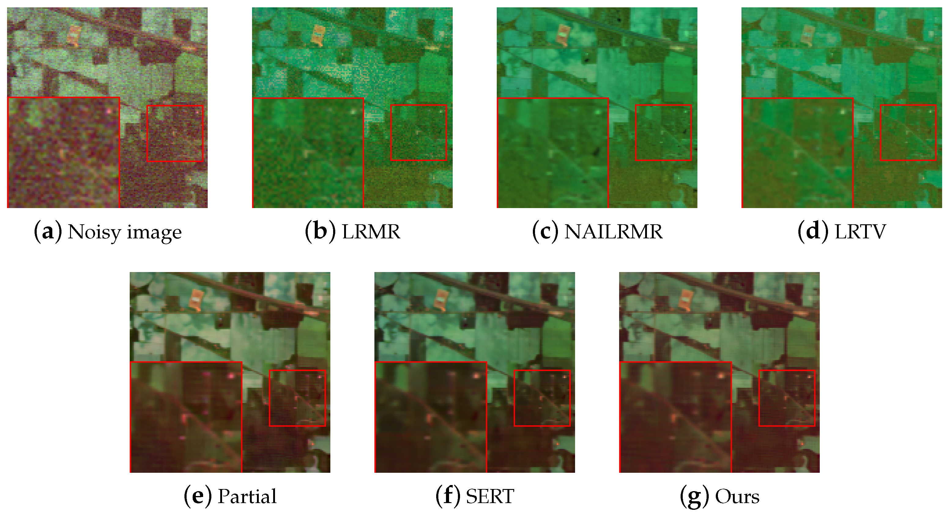
Simialr to [34], the Indian Pines dataset and Pavia University dataset were used as real data to test the performances of five comparison algorithms and the proposed method. The size of the Indian Pines dataset is $145\times 145\times 206$, which was collected by AVIRIS. Meanwhile, the size of the Pavia University dataset is $200\times 200\times 103$. When testing the real datasets, the network trained under Case 2 on the artificially synthesized data was selected as the training model for the two real dataset. Due to the lack of corresponding clean images in real noisy images, a quantitative comparative analysis could not be performed. Therefore, only the visual comparison results of the denoised algorithm and the proposed method are presented here. The visual image-comparison results of each method on the Indian Pines dataset and Pavia University dataset are shown in Figure 6b–g and Figure 7b–g.

Figure 6a is a pseudocolor image from the original HSI Pavia University dataset affected by noise interference, and Figure 6b–g are the denoised results of algorithms LRMR, NAILRMR, LRTV, Partial DNet, SERT, and the proposed algorithm, respectively. According to the previous literature [34], the Pavia University dataset is weakly affected by noise interference. Therefore, the results of traditional denoising algorithms LRMR, NAILRMR, and LRTV are similar to those of deep learning-based denoising methods Partial-DNet and SERT on the Pavia University dataset. After zooming in on all the denoising results, it can be found that our proposed algorithm maintained better and clearer texture details, and some oversmoothing phenomena occurred using the Partial-DNet and SERT methods.

As is well known, the Indian Pines dataset is highly affected by noise interference. Therefore, in Figure 7, it is evident that there are differences between the original noisy image, Figure 7a, and the denoising results of the six algorithms, Figure 7b–g. It can be concluded that the three machine learning-based comparison methods, including LRMR, NAILRMA, and LRTV, cannot completely remove complex noise. After denoising, there are still a large amount of noise in the results. On the contrary, the two methods based on deep learning have much better visual effects than the traditional methods, but they lose many details in some texture areas compared to the proposed method, where there are some oversmoothing phenomena, as shown in Figure 7. Overall, the proposed hyperspectral denoising algorithm based on non-local memory-augmented spectral attention outperforms the comparison methods in terms of visualization on real datasets, with better performances in denoising and detail preservation.

4.3. The Ablation Experiments and Discussions

To obtain the best model, we conducted ablation experiments and confirmed the optimal parameter T on Case 2 data from PC data. In the proposed network, we set a total of T bands, including the current band and its adjacent bands, as inputs to the network to improve the spectral efficiency of the denoising algorithm. Therefore, the input bands T is a key parameter in the denoising network. We explored the influence of T on denoising results, and

Table 3. Results of different T values on Case 3 of the PC data. Bold represents the optimal result.

T	PSNR	SSIM	SAM
T = 15	31.14	0.9733	3.4633
T = 20	31.23	0.9753	3.3062
T = 25	31.88	0.9776	3.2401
T = 30	32.22	0.9792	3.0667
T = 35	32.41	0.9799	3.0055
T = 40	32.32	0.9797	3.0323
T = 45	32.26	0.9790	3.0331

presents the quantitative evaluation results of the algorithm under different spectral band inputs. It can be clearly seen from Table 3 that the denoising performance of this study’s proposed method first improves with the increase in T, and the denoising effect is best when $T=35$. As T further increases, the algorithm performance gradually decreases. Therefore, T was set to 35 here. It could also be demonstrated through parameter experiments that non-local spectral information is crucial for the proposed method.

In addition,

Table 4. Results of ablation experiments on Case 3 of the PC data. Bold represents the optimal result.

	PSNR	SSIM	SAM
o/w	32.22	0.9792	3.0667
w/o	31.23	0.9749	3.3920
Ours	32.41	0.9799	3.0055

provides quantitative evaluation indicators for the ablation experiments of various parts of the network used to analyze the effectiveness of the proposed method. The network mainly consists of two parts. The first part is the spatial information extraction module, which aims to use pixel and spatial relationships to assist in the image restoration performance. To verify its effectiveness, we removed this module from the overall network framework and express it as o/w in the Table 4. From Table 4, we can conclude that its denoising results decreased by about 0.2 dB compared to the original method. The SSIM decreased by 0.0007, and the SAM increased by 0.0612. This is sufficient to prove that the proposed spatial information extraction module is beneficial for hyperspectral denoising tasks. The second part is the non-local memory-enhanced spectral attention module. In order to verify its effectiveness, we removed this module from the overall network framework and express it as w/o in the table. It can be seen that its denoising results decreased by about 1.18 dB compared to the original method; the SSIM decreased by 0.005, and the SAM increased by 0.3865, fully proving the effectiveness of the non-local memory-enhanced spectral attention module. Overall, the above ablation experiments demonstrated the superiority of the proposed network in denoising tasks.

5. Conclusions

We proposed a hyperspectral denoising method that has better robustness against complex noise. Unlike general denoising methods that use spatial–spectral correlations, the proposed method uses a designed cross-band non-local module to search for bands that can provide information supplementation for the current band. Due to the introduction of a memory-augmented module, the proposed network can also remember the detailed information of all bands during training, thereby supplementing the information loss of non-local similarity bands in the global spectral dimension. In addition, the proposed method uses a dense connected network to extract multi-scale spatial information from hyperspectral data. Compared with state-of-the-art denoising algorithms, the proposed network performed better on both synthetic and real data. Unfortunately, the method proposed in this paper is based on 2-D images. An original hyperspectral image is a 3-D image, and the proposed memory-augmented module-based denoising method still unfolds the 3-D image into a 2-D image for processing, losing some irreparable correlation information. In the future, we will explore methods for directly denoising 3D images.

References

1. Yao, H.; Chen, R.; Chen, W.; Sun, H.; Xie, W.; Lu, X. Pseudolabel-Based Unreliable Sample Learning for Semi-Supervised Hyperspectral Image Classification. IEEE Trans. Geosci. Remote Sens. 2023, 61, 5527116. [Google Scholar] [CrossRef]
2. Zheng, X.; Wang, B.; Du, X.; Lu, X. Mutual Attention Inception Network for Remote Sensing Visual Question Answering. IEEE Trans. Geosci. Remote Sens. 2022, 60, 5606514. [Google Scholar] [CrossRef]
3. Zheng, X.; Yuan, Y.; Lu, X. A Deep Scene Representation for Aerial Scene Classification. IEEE Trans. Geosci. Remote Sens. 2019, 57, 4799–4809. [Google Scholar] [CrossRef]
4. Zheng, X.; Cui, H.; Lu, X. Multiple Source Domain Adaptation for Multiple Object Tracking in Satellite Video. IEEE Trans. Geosci. Remote Sens. 2023, 61, 5626911. [Google Scholar] [CrossRef]
5. Zheng, X.; Gong, T.; Li, X.; Lu, X. Generalized Scene Classification from Small-Scale Datasets With Multitask Learning. IEEE Trans. Geosci. Remote Sens. 2022, 60, 5609311. [Google Scholar] [CrossRef]
6. Sun, H.; Li, Q.; Yu, J.; Zhou, D.; Chen, W.; Zheng, X.; Lu, X. Deep Feature Reconstruction Learning for Open-Set Classification of Remote-Sensing Imagery. IEEE Geosci. Remote Sens. Lett. 2023, 20, 6009405. [Google Scholar] [CrossRef]
7. Li, S.; Geng, X.; Zhu, L.; Ji, L.; Zhao, Y. Hyperspectral Image Denoising Based on Principal-Third-Order-Moment Analysis. Remote Sens. 2024, 16, 276. [Google Scholar] [CrossRef]
8. Feng, X.; Tian, S.; Abhadiomhen, S.E.; Xu, Z.; Shen, X.; Wang, J.; Zhang, X.; Gao, W.; Zhang, H.; Wang, C. Edge-Preserved Low-Rank Representation via Multi-Level Knowledge Incorporation for Remote Sensing Image Denoising. Remote Sens. 2023, 15, 2318. [Google Scholar] [CrossRef]
9. Ren, J.; Luo, Y.; Fan, C.; Feng, W.; Su, L.; Wang, H. RAU-Net-Based Imaging Method for Spatial-Variant Correction and Denoising in Multiple-Input Multiple-Output Radar. Remote Sens. 2024, 16, 80. [Google Scholar] [CrossRef]
10. Huang, Z.; Zhu, Z.; Zhang, Y.; Wang, Z.; Xu, B.; Liu, J.; Li, S.; Fang, H. MD3: Model-Driven Deep Remotely Sensed Image Denoising. Remote Sens. 2023, 15, 445. [Google Scholar] [CrossRef]
11. You, H.; Li, Y.; Qin, Z.; Lei, P.; Chen, J.; Shi, X. Research on Multilevel Filtering Algorithm Used for Denoising Strong and Weak Beams of Daytime Photon Cloud Data with High Background Noise. Remote Sens. 2023, 15, 4260. [Google Scholar] [CrossRef]
12. Liu, S.; Liu, T.; Gao, L.; Li, H.; Hu, Q.; Zhao, J.; Wang, C. Convolutional Neural Network and Guided Filtering for SAR Image Denoising. Remote Sens. 2019, 11, 702. [Google Scholar] [CrossRef]
13. Letexier, D.; Bourennane, S. Noise Removal From Hyperspectral Images by Multidimensional Filtering. IEEE Trans. Geosci. Remote Sens. 2008, 46, 2061–2069. [Google Scholar] [CrossRef]
14. Zhang, B.; Aziz, Y.; Wang, Z.; Zhuang, L.; Ng, M.K.; Gao, L. Hyperspectral Image Stripe Detection and Correction Using Gabor Filters and Subspace Representation. IEEE Geosci. Remote Sens. Lett. 2022, 19, 5504005. [Google Scholar] [CrossRef]
15. Othman, H.; Qian, S.E. Noise reduction of hyperspectral imagery using hybrid spatial-spectral derivative-domain wavelet shrinkage. IEEE Trans. Geosci. Remote Sens. 2006, 44, 397–408. [Google Scholar] [CrossRef]
16. Jiao, J.; Gong, Z.; Zhong, P. Dual-Branch Fourier-Mixing Transformer Network for Hyperspectral Target Detection. Remote Sens. 2023, 15, 4675. [Google Scholar] [CrossRef]
17. Chen, G.; Qian, S.E. Denoising of Hyperspectral Imagery Using Principal Component Analysis and Wavelet Shrinkage. IEEE Trans. Geosci. Remote Sens. 2011, 49, 973–980. [Google Scholar] [CrossRef]
18. Maggioni, M.; Katkovnik, V.; Egiazarian, K.; Foi, A. Nonlocal Transform-Domain Filter for Volumetric Data Denoising and Reconstruction. IEEE Trans. Image Process. 2013, 22, 119–133. [Google Scholar] [CrossRef]
19. Ding, M.; Zhou, Y.; Chi, Y. Self-Attention Generative Adversarial Network Interpolating and Denoising Seismic Signals Simultaneously. Remote Sens. 2024, 16, 305. [Google Scholar] [CrossRef]
20. Wang, X.; Bai, X.; Li, G.; Sun, L.; Ye, H.; Tong, T. Noise Attenuation for CSEM Data via Deep Residual Denoising Convolutional Neural Network and Shift-Invariant Sparse Coding. Remote Sens. 2023, 15, 4456. [Google Scholar] [CrossRef]
21. Fan, Y.R.; Huang, T.Z.; Zhao, X.L.; Deng, L.J.; Fan, S. Multispectral Image Denoising via Nonlocal Multitask Sparse Learning. Remote Sens. 2018, 10, 116. [Google Scholar] [CrossRef]
22. Qin, J.; Zhao, H.; Liu, B. Self-Supervised Denoising for Real Satellite Hyperspectral Imagery. Remote Sens. 2022, 14, 3083. [Google Scholar] [CrossRef]
23. Liu, W.; He, C.; Sun, L. Spectral-Smoothness and Non-Local Self-Similarity Regularized Subspace Low-Rank Learning Method for Hyperspectral Mixed Denoising. Remote Sens. 2021, 13, 3196. [Google Scholar] [CrossRef]
24. Fu, Y.; Lam, A.; Sato, I.; Sato, Y. Adaptive Spatial-Spectral Dictionary Learning for Hyperspectral Image Denoising. In Proceedings of the 2015 IEEE International Conference on Computer Vision (ICCV), Santiago, Chile, 7–13 December 2015; pp. 343–351. [Google Scholar] [CrossRef]
25. Xie, Q.; Zhao, Q.; Meng, D.; Xu, Z. Kronecker-Basis-Representation Based Tensor Sparsity and Its Applications to Tensor Recovery. IEEE Trans. Pattern Anal. Mach. Intell. 2018, 40, 1888–1902. [Google Scholar] [CrossRef] [PubMed]
26. Zhao, S.; Yuan, Q.; Li, J.; Shen, H.; Zhang, L. Lunar Hyperspectral Image Destriping Method Using Low-Rank Matrix Recovery and Guided Profile. In Proceedings of the IGARSS 2020–2020 IEEE International Geoscience and Remote Sensing Symposium, Waikoloa, HI, USA, 26 September–2 October 2020. [Google Scholar]
27. He, W.; Zhang, H.; Zhang, L.; Shen, H. Hyperspectral Image Denoising via Noise-Adjusted Iterative Low-Rank Matrix Approximation. IEEE J. Sel. Top. Appl. Earth Obs. Remote Sens. 2015, 8, 3050–3061. [Google Scholar] [CrossRef]
28. Lian, X.; Yin, Z.; Zhao, S.; Li, D.; Lv, S.; Pang, B.; Sun, D. A Neural Network for Hyperspectral Image Denoising by Combining Spatial–Spectral Information. Remote Sens. 2023, 15, 5174. [Google Scholar] [CrossRef]
29. Dou, H.X.; Pan, X.M.; Wang, C.; Shen, H.Z.; Deng, L.J. Spatial and Spectral-Channel Attention Network for Denoising on Hyperspectral Remote Sensing Image. Remote Sens. 2022, 14, 3338. [Google Scholar] [CrossRef]
30. He, W.; Zhang, H.; Zhang, L.; Shen, H. Total-Variation-Regularized Low-Rank Matrix Factorization for Hyperspectral Image Restoration. IEEE Trans. Geosci. Remote Sens. 2016, 54, 178–188. [Google Scholar] [CrossRef]
31. Feng, D.; Wang, X.; Wang, X.; Ding, S.; Zhang, H. Deep Convolutional Denoising Autoencoders with Network Structure Optimization for the High-Fidelity Attenuation of Random GPR Noise. Remote Sens. 2021, 13, 1761. [Google Scholar] [CrossRef]
32. Chang, Y.; Yan, L.; Fang, H.; Zhong, S.; Liao, W. HSI-DeNet: Hyperspectral Image Restoration via Convolutional Neural Network. IEEE Trans. Geosci. Remote Sens. 2019, 57, 667–682. [Google Scholar] [CrossRef]
33. Li, M.; Liu, J.; Fu, Y.; Zhang, Y.; Dou, D. Spectral Enhanced Rectangle Transformer for Hyperspectral Image Denoising. In Proceedings of the 2023 IEEE/CVF Conference on Computer Vision and Pattern Recognition (CVPR), Vancouver, BC, Canada, 17–24 June 2023; pp. 5805–5814. [Google Scholar] [CrossRef]
34. Yuan, Y.; Ma, H.; Liu, G. Partial-DNet: A Novel Blind Denoising Model With Noise Intensity Estimation for HSI. IEEE Trans. Geosci. Remote Sens. 2022, 60, 5505913. [Google Scholar] [CrossRef]
35. Wei, K.; Fu, Y.; Huang, H. 3-D Quasi-Recurrent Neural Network for Hyperspectral Image Denoising. IEEE Trans. Neural Netw. Learn. Syst. 2021, 32, 363–375. [Google Scholar] [CrossRef]
36. Dong, W.; Wang, H.; Wu, F.; Shi, G.; Li, X. Deep Spatial–Spectral Representation Learning for Hyperspectral Image Denoising. IEEE Trans. Comput. Imaging 2019, 5, 635–648. [Google Scholar] [CrossRef]
37. Yuan, Q.; Zhang, Q.; Li, J.; Shen, H.; Zhang, L. Hyperspectral Image Denoising Employing a Spatial–Spectral Deep Residual Convolutional Neural Network. IEEE Trans. Geosci. Remote Sens. 2019, 57, 1205–1218. [Google Scholar] [CrossRef]
38. Maffei, A.; Haut, J.M.; Paoletti, M.E.; Plaza, J.; Bruzzone, L.; Plaza, A. A Single Model CNN for Hyperspectral Image Denoising. IEEE Trans. Geosci. Remote Sens. 2020, 58, 2516–2529. [Google Scholar] [CrossRef]
39. Han, J.; Pan, C.; Ding, H.; Zhang, Z. Double-Factor Tensor Cascaded-Rank Decomposition for Hyperspectral Image Denoising. Remote Sens. 2024, 16, 109. [Google Scholar] [CrossRef]
40. Yang, F.; Chen, X.; Chai, L. Hyperspectral Image Destriping and Denoising Using Stripe and Spectral Low-Rank Matrix Recovery and Global Spatial-Spectral Total Variation. Remote Sens. 2021, 13, 827. [Google Scholar] [CrossRef]
41. Feng, X.; Zhang, W.; Su, X.; Xu, Z. Optical Remote Sensing Image Denoising and Super-Resolution Reconstructing Using Optimized Generative Network in Wavelet Transform Domain. Remote Sens. 2021, 13, 1858. [Google Scholar] [CrossRef]
42. Zhang, J.; Cai, Z.; Chen, F.; Zeng, D. Hyperspectral Image Denoising via Adversarial Learning. Remote Sens. 2022, 14, 1790. [Google Scholar] [CrossRef]
43. Wang, Y.; Xu, S.; Cao, X.; Ke, Q.; Ji, T.Y.; Zhu, X. Hyperspectral Denoising Using Asymmetric Noise Modeling Deep Image Prior. Remote Sens. 2023, 15, 1970. [Google Scholar] [CrossRef]
44. Cao, X.; Fu, X.; Xu, C.; Meng, D. Deep Spatial-Spectral Global Reasoning Network for Hyperspectral Image Denoising. IEEE Trans. Geosci. Remote Sens. 2022, 60, 5504714. [Google Scholar] [CrossRef]
45. Yu, J.; Liu, J.; Bo, L.; Mei, T. Memory-Augmented Non-Local Attention for Video Super-Resolution. In Proceedings of the 2022 IEEE/CVF Conference on Computer Vision and Pattern Recognition (CVPR), New Orleans, LA, USA, 18–24 June 2022; pp. 17813–17822. [Google Scholar] [CrossRef]
46. Cao, C.; Yu, J.; Zhou, C.; Hu, K.; Xiao, F.; Gao, X. Hyperspectral Image Denoising via Subspace-Based Nonlocal Low-Rank and Sparse Factorization. IEEE J. Sel. Top. Appl. Earth Obs. Remote Sens. 2019, 12, 973–988. [Google Scholar] [CrossRef]
Figure 1. Structure of the denoising method proposed in this paper.
Remotesensing 16 01937 g001
Figure 2. Architecture of DCM.
Remotesensing 16 01937 g002
Figure 3. Structure of the MAN.
Remotesensing 16 01937 g003
Figure 4. Pseudocolor results (red: band 17, green: band 27, and blue: band 57) of Case 2 on the WDC dataset. (a) Clean. (b)Noisy. (c) LRMR. (d) NAILRMR. (e) LRTV.(f) Partial-DNet. (g) SERT. (h) Ours.
Remotesensing 16 01937 g004
Figure 5. Pseudocolor results (red: band 17, green: band 27, and blue: band 57) of Case 2 on the Pavia Center dataset. (a) Clean. (b) Noisy. (c) LRMR. (d) NAILRMR. (e) LRTV.(f) Partial-DNet. (g) SERT. (h) Ours.
Remotesensing 16 01937 g005
Figure 6. Pseudocolor results (red: band 77, green: band 2, and blue: band 1) of Case 2 on the Pavia Unversity dataset. (a) Noisy image. (b) LRMR. (c) NAILRMR. (d) LRTV. (e) Partial-DNet. (f) SERT. (g) Ours.
Remotesensing 16 01937 g006
Figure 7. Pseudocolor results (red: band 1, green: band 109, and blue: band 203) of Case 2 on the Indian Pines data. (a) Noisy image. (b) LRMR. (c) NAILRMR. (d) LRTV. (e) Partial-DNet. (f) SERT. (g) Ours.
Remotesensing 16 01937 g007