Abstract
Wildfires present a significant threat to ecosystems and human life, requiring effective prevention and response strategies. Equally important is the study of post-fire damages, specifically burnt areas, which can provide valuable insights. This research focuses on the detection and classification of burnt areas and their severity using RGB and multispectral aerial imagery captured by an unmanned aerial vehicle. Datasets containing features computed from multispectral and/or RGB imagery were generated and used to train and optimize support vector machine (SVM) and random forest (RF) models. Hyperparameter tuning was performed to identify the best parameters for a pixel-based classification. The findings demonstrate the superiority of multispectral data for burnt area and burn severity classification with both RF and SVM models. While the RF model achieved a 95.5% overall accuracy for the burnt area classification using RGB data, the RGB models encountered challenges in distinguishing between mildly and severely burnt classes in the burn severity classification. However, the RF model incorporating mixed data (RGB and multispectral) achieved the highest accuracy of 96.59%. The outcomes of this study contribute to the understanding and practical implementation of machine learning techniques for assessing and managing burnt areas.
1. Introduction
Wildfires pose an escalating threat to wildlife ecosystems, contributing to the exacerbation of global warming, as well as endangering human life and causing significant material damage [1]. Consequently, the need to combat this threat has intensified, leading to numerous studies in the past decade focusing on optimizing wildfire prevention [2], wildfire detection and monitoring [3], and post-fire analysis [4].
While preventing and detecting wildfires is crucial, assessing their aftermath is equally vital. Accurately delineating fire-affected areas offers multiple benefits, including ecosystem monitoring [5,6,7]. Vegetation ignition, whether through direct flames or wildfire spread, poses a significant threat to wildlife [8,9]. Habitat destruction disrupts ecosystems, emphasizing the need to monitor and study the impacts [10,11,12]. Mapping burnt areas also aids in developing fire risk models [13] because of the various factors influencing fire risk [14,15].
Ground-level data acquisition, often affected by limited access to extensive and remote wildfire-affected areas, has become slow and inefficient [16]. However, advancements in the remote sensing of fire-affected vegetation using unmanned aerial vehicles (UAVs) or satellite imagery have enabled access to high-resolution data [17]. These data can be used for various purposes, including identifying and mapping burnt areas and tracking live wildfires. Satellites, widely employed in remote sensing studies for burnt area identification [18], are favored for their easy data availability, granting access to both pre- and post-fire data and simplifying active fire monitoring [19].
Optical sensors or cameras on manned aircraft, UAVs, or satellites gather aerial data of burnt areas. Manned aircraft were initially employed for active forest fire detection, complementing ground-based fire watchtowers and patrols [20]. However, UAVs offer significant advantages, such as eliminating human operation in hazardous conditions and overcoming flight duration, safety, and pilot-related costs [21,22]. UAV employment goes beyond fire detection, being useful for fire prevention by creating fire risk maps through vegetation monitoring and post-fire analysis by mapping burnt areas [23]. Their application extends to vegetation monitoring in diverse contexts [24,25], being optimal for monitoring small- to medium-sized areas [26]. However, limited endurance due to power constraints often requires specific flight campaigns for such high spatial resolution data [27].
Satellite imaging platforms offer readily available and, in certain cases, free data from different sensors, allowing global-scale studies with moderate spatial resolution due to their continuous orbit [28]. Unlike UAVs, satellite data acquisition is not constrained by time or space, but it does involve a revisiting period, the interval between consecutive observations of the same area [29]. When comparing UAV data resampled to match satellite spatial resolution for burnt area monitoring, both platforms yield similar accuracy results for the same study area [30]. However, data accessibility differs significantly [31]. UAV data collection is more time-consuming and costly [32], especially for multi-temporal analysis, requiring multiple trips.
While some studies exclusively focus on the visible spectrum using RGB sensors for burnt area detection [33,34], the availability of data beyond the visible range from spectral sensors enables diverse methods for distinguishing burnt from non-burnt areas. Spectral indices, computed from values across spectral bands, are widely applied in satellite- and UAV-based studies for vegetation and burnt area detection [35]. Highly effective and prevalent among these indices are the normalized difference vegetation index (NDVI) [36] and the normalized burn ratio (NBR) [37]. Both rely on specific bands in the infrared spectrum, using the near-infrared (NIR) and, in the case of NBR, the shortwave infrared (SWIR) spectra. The prominence of these infrared regions in wildfire and burnt area detection increased when it was found that burnt areas exhibit reduced NIR reflection and increased SWIR reflection, attributed to foliage destruction and reduced water content [17]. Furthermore, these indices can be used in a different manner by capturing pre- and post-fire vegetation imagery and then subtracting index values to compute the delta normalized difference vegetation index (dNDVI) and the delta normalized burn ratio (dNBR) [18,30].
Following data acquisition, processing, and index selection for burnt area identification, a classification method is necessary. Among the various classification methods employed for this purpose, the literature predominantly favors the application of machine learning methods [18]. Among these methods, the random forest (RF) classifier stands out because of its robustness and versatility. It has consistently demonstrated good results for both local and global burnt area classification and burn severity assessment, particularly excelling in multispectral data classification [38,39,40,41,42]. The support vector machine (SVM) is another commonly used method for burnt area classification [43]. Artificial neural networks have been widely employed as classifiers in previous burnt area mapping studies [44,45,46] because of their versatility and widespread use. Bayesian algorithms applied to multispectral data are used to map and delineate perimeters resulting from wildfires in various regions, including North America, Siberia, and the Canary Islands [47,48,49]. While the use of machine learning methods represents the predominant approach for burnt area mapping, simple alternatives, such as threshold estimation for vegetation indices segmentation, have also been explored [34].
The main objective of this article is to compare the performance of SVM and RF models in classifying burnt areas using RGB and multispectral data acquired from a UAV in a post-fire scenario. The study aims to investigate the effectiveness of distinguishing burnt from unburnt areas and performing fire severity classification using datasets created from both types of imagery (RGB, multispectral, and their fusion). The article focuses on the qualitative and quantitative evaluation of supervised machine learning methods applied to these datasets.
2. Materials and Methods
2.1. Study Area
The area explored in this study is a forested region located in northeast Portugal (Figure 1a) within the Vila Real district (41°20–50.1″N, 7°35–38.9″W, altitude 630 m). On 31 August 2022, a wildfire occurred near Parada do Pinhão in the municipality of Sabrosa, resulting in the destruction of approximately 40 hectares of forested land. The study area specifically encompasses the location where the fire originated (Figure 1c, which is predominantly composed of shrubs and maritime pines (Pinus pinaster Aiton), as seen in an orthomosaic of 2019 (Figure 1b).
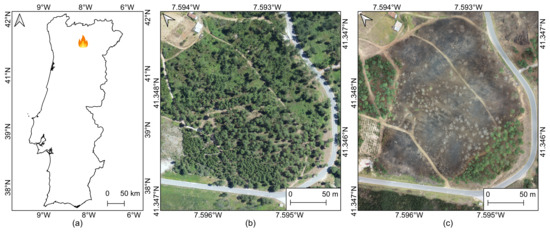
Figure 1.
Location of the fire event within mainland Portugal (a) and an overview of the study area in 2019 (b) and 2023 (c) after the fire occurrence.
2.2. Remote Sensing Data
UAV-based remote sensing data were collected using a Phantom 4 Pro V2.0 (DJI, Shenzhen, China). The multi-rotor UAV was equipped with two imaging sensors: an RGB sensor, which has a resolution of 20 MP and is attached to a 3-axis gimbal, and a Sequoia multispectral sensor (Parrot SA, Paris, France). The multispectral sensor is capable of capturing data with a resolution of 1.2 MP in the green (550 nm ± 40 nm), red (660 nm ± 40 nm), red edge (735 nm ± 10 nm), and NIR (790 nm ± 40 nm) parts of the electromagnetic spectrum. While in flight, a sensor mounted on the UAV collected irradiance data, and reflectance data were acquired from a pre-flight calibration target. Both irradiance and reflectance data were employed for radiometric calibration. A flight campaign was carried out on 19 February 2023, five to six months after the fire disturbance. At that time, there was minimal lowland vegetation regeneration. The mission was designed to capture imagery with 80% longitudinal overlap and 70% lateral overlap at a height of 80 m above the UAV take-off point, covering a total area of eight hectares.
The acquired UAV imagery was processed using a Pix4Dmapper Pro (Pix4D SA, Lausanne, Switzerland). Common tie points were estimated between images to compute a dense point cloud with high point density. Subsequently, the point cloud was interpolated to generate orthorectified raster products. This was achieved by employing the inverse distance weighting (IDW) method with noise filters and surface smoothing. From the RGB imagery (0.024 m spatial resolution), only the orthomosaic was used among the generated products. For the multispectral data (0.094 m spatial resolution), reflectance maps were computed for each band after radiometric calibration. These reflectance maps were used to derive various orthorectified raster products representing vegetation indices, based on literature for burned areas monitoring and vegetation detection (Section 2.3). Data alignment from both sensors was accomplished using identifiable points in the imagery from both sensors, including natural features and artificial targets within the study area.
Furthermore, Sentinel-2 multispectral instrument (MSI) data were used for burn severity mapping by capturing information before and after the occurrence of the fire. These data were used to calculate the pre-fire and post-fire NBR, using bands eight (NIR) and twelve (SWIR). The pre-fire and post-fire NBRs were then subtracted to obtain a dNBR specifically for the fire that took place within the study area. This dNBR was employed for the classification of burn severity. The entire process was conducted using Google Earth Engine [50]. The pre-fire period was defined as a time frame with cloud-free data between 1 July and 25 August 2022, while the post-fire period corresponded to 5 and 30 September 2022. By performing these calculations, burn severity across the entire extent of the fire could be estimated, as depicted in Figure 2.
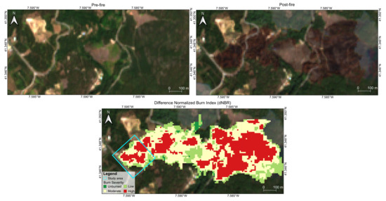
Figure 2.
Overview of the area before and after the fire occurrence (from Sentinel-2 data), along with the fire severity classes from the delta normalized burn ratio (dNBR) of the entire fire extent. Blue polygon corresponds to the UAV surveyed area.
2.3. Computation of Spectral Indices
With the use of digital cameras, the data obtained from each band could be effectively employed in arithmetic operations combining the various available bands, resulting in new and distinctive parameters, referred to as spectral indices. Spectral indices hold significant importance in the realm of remote sensing as they serve to enhance or isolate specific spectral characteristics of the analyzed features or those intended to be identified. Within the field of environmental remote sensing, these indices are often referred to as vegetation indices because of their frequent application in vegetation analysis. The calculation of the NBR and dNBR indices, which are used as a support tool for the labeling of the datasets, are calculated as
While there exist numerous indices employed in remote sensing, a set of seven spectral indices, using bands from the visible spectrum, was selected (Table 1). These indices were chosen based on their established capability to discriminate vegetation and distinguish different characteristics [34,51,52]. Alongside these indices, the normalized red (Rn), green (Gn), and blue (Bn) were also used. These were calculated by dividing a given band (red, green, or blue) by the sum of the pixel values of all bands. This calculation results in a normalized value that considers the relative contribution of the red, green, and blue channels, helping to create a balanced representation of each component in the image.

Table 1.
Vegetation indices computed from RGB data. R: red; G: green; B: blue.
Multispectral sensors capture data from other electromagnetic spectrum regions, allowing the computation of spectral indices by combining bands from both the visible and infrared parts of the spectrum. Table 2 presents a collection of indices used in this study and commonly employed in remote sensing, with many of them using data beyond the visible spectrum, specifically in the NIR and red edge portions.
Table 2.
Vegetation indices computed from multispectral data. G: green; R: red; RE: red edge; N: near-infrared; .
2.4. Dataset Creation
The orthorectified raster products generated from the processing of UAV data served as the basis for constructing datasets, comprising a total of 20 distinct features derived from the indices computed from both multispectral and RGB data (Table 1 and Table 2) as well as the normalized bands from the RGB imagery and the reflectance from the four bands of the multspectral sensor (green, red, red edge, and NIR). These features were employed as predictors for the classification tasks conducted in this study.
Following the creation of mosaics for all products derived from the RGB and multispectral data, the datasets were prepared. The objective was to generate three distinct datasets: one composed of the 10 indices and bands computed from the RGB data, another consisting of the 10 multispectral indices and bands, and a third dataset encompassing all 20 features. This separation (i) allowed a comparative analysis between RGB and multispectral features in terms of their effectiveness in detecting and classifying the severity of burnt areas and (ii) enabled the evaluation of whether the combination of data from both sensors can yield an improved performance when applied in a classification algorithm. Given that the spectral indices were separated into individual raster layers, they needed to be aggregated into three composite raster images, where each band represented a specific feature. As a result, two rasters were created for the RGB and multispectral groups, each containing 10 bands, while an additional raster was generated to combine all 20 bands from both the RGB and multispectral datasets. This aggregation process was conducted within QGIS.
The subsequent step in constructing the three datasets involved extracting the data from the imagery. This was achieved by creating several 2 × 2 m polygons in the form of a vector layer, overlapping them onto the designated image locations and assigning two values to each polygon, representing the classes for two classification scenarios: (1) burn severity classification, in which each polygon was classified into three severity classes (unburnt, mildly burnt, and severely burnt), and (2) burnt classification, in which each polygon was classified as either burnt or unburnt. The dNBR, derived from Sentinel-2 MSI data (Section 2.2), served as a ground-truth reference to some extent for determining the burn severity of specific parts of the study area. However, because of differences in spatial and temporal resolutions between the Sentinel-2 and the UAV data, variations in the overlapping classification arose, and a manual classification override was made through a photo interpretation of the RGB orthomosaic for certain polygons.
A total of 417 polygons were created: 206 in unburnt areas, 105 in mildly burnt areas, and 106 in severely burnt areas. With the annotated polygons, the data from the three concatenated raster products could be extracted. To accomplish this, points were created inside each polygon, with each point representing a single pixel containing the information from all UAV-based data in the aggregated image being analyzed. These points were used for dataset creation as well as for the classification procedure. A total of 150 random points were generated within each polygon, resulting in a total of 68,850 points. Subsequently, the data were extracted from the three raster products containing the features to use in each dataset using the generated points. The process was performed three times to obtain three separate vector files: one file with RGB indices information containing 10 features corresponding to the 10 RGB indices at each point, another file with 10 features consisting of multispectral information, and finally, a file combining all 20 RGB and multispectral indices and bands. Each of these files also included the associated classes (burnt area detection and burn severity) of the polygons in which the randomly generated points were located. Furthermore, the mean value of each feature was extracted from the 417 polygons to evaluate the distribution of data within each feature.
2.5. Implemented Methods
The implementation of the machine learning classification methods was carried out using the TrainImageClassifier function from Orfeo ToolBox (OTB) [63] in QGIS. The TrainImageClassifier function incorporates both SVM and RF classifiers through a graphical user interface (GUI), with the chosen classification method being one of the required parameters for execution. OTB implements several classification methods that use the OpenCV library [64], including the RF algorithm. For the SVM, the LibSVM library [65] is used. The workflow of TrainImageClassifier is straightforward by specifying the input data and the training and testing set options and by selecting the classification method along with the respective parameters.
To further explain the parameters required for this function, three categories were involved. In the input data section, the selection was made for images containing the data divided into bands, where each band corresponded to an independent variable, and the points with class information were also selected. The parameters for the training and validation samples were specified with a value of inserted for both, indicating that there was no limit on the sample size and ensuring that the created models used all the samples from the datasets. Moreover, the training–validation ratio was defined with a 30% validation split for all models. Depending on the model being created, either the severity class or the burn detection class was chosen as the target class to be classified. The function was parameterized to perform an under-sampling of the dataset in both the training and validation sets, ensuring that all classes had the same number of samples as the class with the fewest samples, addressing dataset imbalance. After under-sampling was applied, the total number of samples in the datasets for burnt area classification was 67,800, with 47,460 samples used for model training and 20,340 for validation, while for the severity classification, the total number of samples was 52,200, with 36,540 samples used for model training and 15,660 used for validation. The final section of the TrainImageClassifier GUI was specific to the chosen classification method. After selecting either the SVM or the RF classifiers, the respective model parameters were displayed. The outputs of this function were the created model and a list of performance metrics along with the confusion matrix.
For optimal classification results, an algorithm to automate parameter optimization in machine learning methods was developed in Python using the Scikit Learn library [66]. The script conducts hyperparameter tuning using 5-fold cross-validation and a grid search algorithm across the three datasets. The grid search algorithm explores all possible parameter combinations and selects the best configuration based on a predefined metric. In this study, the average F1-score was chosen as the evaluation metric. Cross-validation was introduced to ensure the results are representative of the entire dataset. In this implementation, 5-fold cross-validation was used to enhance computational efficiency. These algorithms were applied to determine the optimal parameters for both severity analysis, considering three severity classes, and burnt area detection, considering two classes.
For the RF classifier, five parameters were optimized: n_estimators, the number of threes in the forest, tested with values 100, 200, and 500; max_depth, the maximum depth of each decision tree, tested with values 5, 10, 20, and 30; min_samples_split, the minimum number of samples required to split an internal node, tested with values 2, 5, and 10; min_samples_leaf, the minimum number of samples required to be at a leaf node, tested with values 5, 10, 15, and 40; and max_features, the maximum number of features to consider when splitting a node, tested with values (square root of the total number of features in the dataset), 2, and 5. Three parameters were optimized for the SVM classifier: kernel, which specifies the kernel type to be used, a linear kernel or a radial basis function (RBF) kernel; the cost parameter (C), tested with values 0.1, 1, and 10; and gamma, the RBF kernel gamma coefficient, tested with values 0.01, 0.1, and 1. The hyperparameter tuning of the RF and SVM models resulted in the 12 combinations of parameters presented in Table 3 and Table 4, used for constructing the corresponding model.
Table 3.
Selected parameters resulting from the hyperparameter tuning for the random forest models in each classification scenario and dataset. RGB: red, green, blue; MSP: multispectral.
Table 4.
Selected parameters resulting from the hyperparameter tuning for the support vector machine models in each classification scenario and dataset. RGB: red, green, blue; MSP: multispectral; RBF: radial basis function.
The optimized parameters obtained in the hyperparameter tuning for each model were then inserted into the corresponding parameter slots of the TrainImageClassifier function. All models were tested 10 times, with each test using randomly distributed training and testing data with a 30% testing split. Once the classification models were created, another OTB function was used to classify the fully aggregated images with the spectral information. These images were used to build the models from each classifier and dataset combination, which were then applied to classify each pixel of the entire study area. This process offered a qualitative output that allowed the visualization of the classification results from the various models, demonstrating the areas and specific details that were correctly or incorrectly classified by these models.
2.6. Performance Metrics
To gain a more comprehensive and conclusive understanding of each model’s and classifier’s performances, several metrics were calculated from the confusion matrix obtained in the validation phase. These encompassed precision, recall, F1-Score, overall accuracy, and Cohen’s kappa coefficient.
Precision represents the ratio of samples correctly classified as positives (true positives) to the total instances predicted as positive, whether correct (TP) or incorrect (false positives). This metric provides insights into areas where the model can improve by minimizing false positive classifications, thus maximizing precision. In turn, recall indicates the ratio of instances correctly classified as positives (true positives) to the total number of instances that are, in fact, positive, obtained from the sum of instances correctly classified as positive and incorrectly classified as negative (false negatives). It allows monitoring the number of false negative predictions, as a decrease in this number corresponds to an increase in recall. In supervised machine learning classification methods, the goal is to optimize both precision and recall metrics by minimizing false positive and false negative predictions. However, it is crucial to assess the balance between these metrics; emphasizing one could potentially compromise the other. To address this balance, the F1-score is employed. It serves as the harmonic mean of precision and recall metrics.
Cohen’s kappa coefficient and the overall accuracy differ from the precision, recall, and F1-score, as they analyze the overall performance of the models rather than the performance for each class individually. Overall accuracy is a widely used metric for evaluating machine learning classifier performance. It provides a measure of how many correct predictions the model makes out of the total number of samples to predict. Cohen’s kappa coefficient, in contrast, is a distinctive statistic that quantifies the normalized agreement (ranging from to 1) between the observed accuracy of the model () and the expected accuracy (). What makes unique is the use of the expected accuracy, which is calculated as the proportion of agreement between results generated by a random classifier and the actual labeled ground truth. This metric measures how closely the instances classified by the machine learning classifier align with the ground truth labels while considering the agreement that would be expressed by chance. It is particularly valuable for directly comparing different models in the context of the same classification task.
3. Results
3.1. Dataset Analysis
Figure A3a,b (Appendix A) present the boxplots of the RGB indices (visual representation in Figure A1), showing the variation within each severity class. Upon analyzing the normalized RGB bands, it becomes evident that the green band exhibits higher values in unburnt areas while showing similar lower values in burnt classes. Conversely, the blue band displays lower values in unburnt areas and increasingly higher values in the mildly and severely burnt classes. The normalized red band shows comparable values across all classes, with a tendency for slightly higher values in the mild severity class. When considering the remaining indices computed from the RGB data, unburnt areas generally manifest higher values within their interquartile range (IQR), except for EGIR. Concerning the burnt classes, the severely burnt class demonstrates higher values than the mild burnt class for GRVI and VARI, while the opposite trend is observed for GBVI and EGIR. As for the variation in the values of the features computed from the multispectral data (Figure A3c and visual representation in Figure A2), it is observed that most of them present higher values in the unburn class, with the exception of the green and red bands, which demonstrate a slight overlap with the burnt classes. The class order is followed by the mild burnt class and then the severely burnt class, with the exception of GRVI, which presents an opposing behavior for the burnt classes.
3.2. Quantitative Results
3.2.1. Burnt Area Detection
The mean outcomes of each metric computed for the binary classification, specifically for burnt area detection, are presented in Table 5. Furthermore, the table presents the results of the two classification methods used for burnt area detection, namely, the RF and the SVM algorithms. The combined usage of RGB and multispectral features in the RF model provided the best results, yielding the highest values for all the metrics. In terms of the SVM model outcomes, the model trained on the multispectral dataset achieved the best results with this classifier, with an overall accuracy of 97.2%. However, the models trained on the other two datasets also offered similar performances to the multispectral dataset. Specifically, the RGB dataset achieved an overall accuracy of 94.9%, while the dataset combining data from both sensors had an overall accuracy of 96.4%.
Table 5.
Random forest (RF) and support vector machine (SVM) burnt area classification performance for each dataset. Best performance model for each algorithm is in bold. Values represent the average of 10 tests. RGB: red, green, blue; MSP: multispectral; OA: overall accuracy.
3.2.2. Burn Severity Mapping
For the severity mapping, the mean outcomes for each metric are presented in Table 6. These results encompass three classes representing different levels of burn severity: unburnt, mild severity, and severely burnt. The analysis involved three datasets, each containing either RGB indices, multispectral indices, or both. Moreover, the table offers a direct comparison between the two employed classification methods, specifically the RF and SVM algorithms, for the burn severity classification within the study area.
Table 6.
Random forest (RF) and support vector machine (SVM) burn severity classification performance for each dataset. Best performance model for each algorithm is in bold. Values represent the average of 10 tests. RGB: red, green, blue; MSP: multispectral; OA: Overall Accuracy.
3.3. Qualitative Results
3.3.1. Burnt Area Detection
Figure 3a provides an overview of the classification maps, highlighting differences among the results obtained from the various datasets analyzed when employing the top-performing RF and SVM models. The models trained solely with features computed from RGB data exhibit a larger burnt area. Contrarily, models trained with multispectral data demonstrate a smaller burnt area. The use of all features from both sensors leads to opposing results. While applying the SVM model results in a larger burnt area, the RF model showcases a smaller burnt area.

Figure 3.
Burnt area classification for the different datasets and classifiers (a), orthomosaic of the study area (b), and burnt and unburnt areas based on the delta normalized burn ratio (c).
3.3.2. Burn Severity Analysis
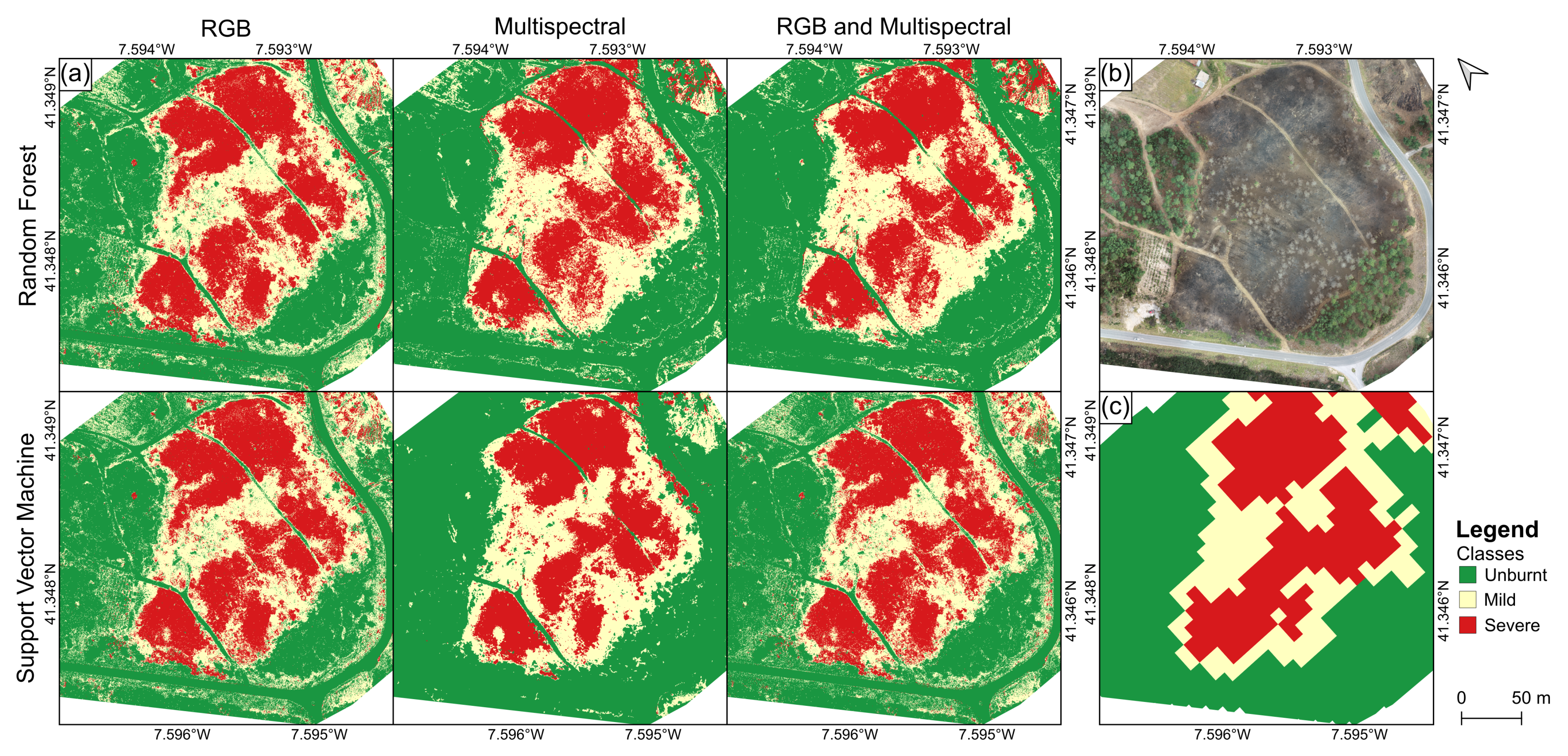
The qualitative results for the severity classification (Figure 4a) were expected to exhibit a slight reduction in performance compared to the results of binary classification for burnt area detection, as quantified in Section 3.2.2.
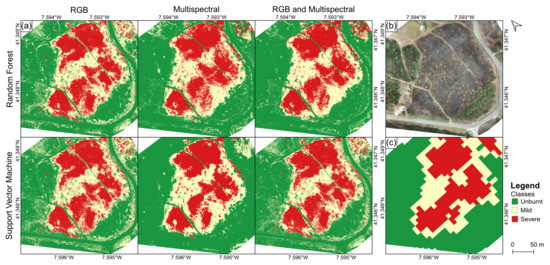
Figure 4.
Burn severity classification for the different datasets and classifiers (a), orthomosaic of the study area (b), and burnt severity based on the delta normalized burn ratio (c).
The classification maps presented in Figure 4 reveal distinct class areas, influenced by the used features and classifier. The application of RGB data identified roughly most of the examined area as unburnt, with a minor variance between mild and high severity in both classifiers. In the SVM model, a larger region was classified as high severity, while the RF model exhibited the opposite trend. However, both models indicated a larger area classified as mild severity as opposed to high severity. When employing models trained with multispectral data, a larger unburnt area was verified in both RF and SVM. In contrast, using features from both sensors, the RF model depicted a larger unburnt area, while the SVM model showed a larger mild severity region compared to severely burnt areas.
4. Discussion
The dataset analysis (Section 3.1) highlights a more pronounced class separation in the multispectral data, whereas the RGB data exhibit overlap between mildly and severely burnt classes, potentially complicating fire severity classification. However, both data types distinctly differentiate burnt from unburnt areas. The multispectral bands align with the findings reported by Pérez-Rodríguez et al. [67] and some indices from Arnett et al. [68] in satellite imagery. Variations in multispectral indices (Figure A3c) allow a comparison with the RGB data. Multispectral indices follow a similar pattern to RGB indices, except for the green and red bands, which slightly overlap with burnt classes, with unburnt areas exhibiting higher values, followed by the mildly burnt class and then the severely burnt class. Notably, GRVI shows different behaviors for the burnt classes.
4.1. Burnt Area Detection
In what concerns burnt area detection, the RF model yielded the best results when using all features (Table 5). The RGB-only dataset shows a strong performance, achieving over 95% across all metrics, including the index, indicating that the accuracies of these models are not merely due to chance. In contrast, the SVM model combining data from both sensors experiences a drop in performance, with the multispectral dataset having the best performance. This implies that the key distinction between RF and SVM outcomes in burnt area classification is that while integrating RGB and multispectral data enhances RF model accuracy moderately, it diminishes SVM model accuracy. This suggests that for SVM, an increase in the number of features negatively impacts burnt area classification.
Regarding the qualitative results for RF classification (Figure 3), the model trained with the RGB dataset effectively outlines the burned area. Nevertheless, some misclassification occurs in unburnt regions, leading to noise-like patterns in these areas. This noise is primarily due to misclassified burnt pixels, aligning with the model performance test findings. Notably, among the RF models, the one trained with the RGB dataset exhibits the lowest performance. Although the performances of the multispectral dataset and the dataset combining data from both sensors are similar, upon closer examination, the RGB & MSP model appears slightly superior, offering a more accurate classification compared to the multispectral model when compared with the ground truth (Figure 3c).
The qualitative results of the SVM classifier (Figure 3) reveal variations among the classification outcomes of different models. It is evident that the model trained with multispectral data exhibits superior performance, in line with the observations outlined in Table 5. However, even when the results with features from RGB or both sensors display increased noise-like patterns, they should not be considered poor, as they effectively delineate the burnt area. Misclassification errors are primarily concentrated in the unburnt regions of the study area. While all datasets demonstrate the ability to differentiate between most burnt and unburnt areas, the multispectral data show a reduced number of misclassifications. This highlights the superior performance of multispectral data in this SVM classification scenario and underscores that adding RGB features alongside the multispectral dataset does not improve the classification outcomes.
The larger burnt area observed with only RGB data (Figure 3a) can be attributed to false positive classifications in non-burned regions, notably on the western side of the study area (Figure 3b). When comparing these results with the dNBR data derived from the Sentinel-2 MSI (Figure 3c), a similar area is obtained if areas classified as low severity are considered unburnt. The use of multispectral data significantly improves the accuracy of burnt area classification, especially in the SVM model, with slight improvements observed when combining data from both sensors in the RF classifier.
While the study areas differ, it is worth noting that the results of this study can be compared to those reported by Petropoulos et al. [43] in terms of burnt area delineation. In their study, employing an SVM with an RBF kernel on Landsat TM multispectral imagery with four or six spectral bands, they achieved 100% accuracy for burnt area detection. In this study, the SVM model trained with multispectral data achieved an overall accuracy of 97.2%, which is slightly lower. This variance in performance can be attributed to differences in platforms, sensors, and spatial resolution. Furthermore, the RF model’s overall accuracy of 99.05% for multispectral imagery is closer to the results of Petropoulos et al. [43].
4.2. Burn Severity Mapping
Regarding the burnt severity results with optimized RF models shown in Table 6, they are generally robust for the models employing multispectral data, surpassing the performance of the RGB-only dataset. However, the RGB dataset struggles to distinguish between mildly and severely burnt classes. Despite this, the RF model trained with RGB features exhibits a high accuracy in classifying unburnt samples, achieving an F1-score exceeding 90%, consistent with its performance in burnt area classification.
Among the two datasets encompassing multispectral data, combining RGB data enhances the RF classification performance slightly (Table 6). The dataset including all features achieves the best results across all metrics. It is important to highlight that the difference between the multispectral-only and all-features datasets is minimal, with variations in the F1-score and overall accuracy within a maximum of 1.51%, primarily observed in the F1-score of the severely burnt class. The SVM results favor the multispectral dataset in all metrics and classes when compared to the other datasets. While the RGB dataset excels in the unburnt class, with an F1-score exceeding 92%, it faces challenges in distinguishing between mild and severe classes. This difficulty is consistently observed in all SVM-based severity models, paralleling the RF issue with the RGB dataset. In contrast, the SVM model relying solely on multispectral data demonstrates the highest performance, aligning with its performance in the burnt area classification. The models using all features and multispectral-only data mirror the RF performance. However, the addition of RGB data slightly hampers the RBF kernel SVM’s performance.
The overall results from the RF and SVM classifiers (Table 6 and Figure 4) suggest that RF excels in classifying burnt area severity when multispectral data are included. However, for models based on RGB data, both RF and SVM exhibit similar accuracy across all performance metrics. Notable differences emerge in models trained with multispectral and mixed datasets. RF significantly outperforms SVM, achieving a 96.59% accuracy for multispectral data compared to SVM’s 83.03%. It is noteworthy that throughout the severity analysis, RF consistently outpaces SVM in computational speed, consistent with prior studies [69,70].
Qualitative RF results (Figure 4a) support the quantitative findings. The RGB model struggles to differentiate between mildly and severely burnt classes, leading to distinct shapes of severely burnt areas, unlike the more consistent shapes produced by the multispectral models. These models maintain uniform burnt area shapes, particularly for high-severity burnt areas characterized by darker soil patches from burnt vegetation. However, despite this limitation, the RGB model effectively identifies most unburnt areas but occasionally misclassifies them as mild severity, including bare soil areas. Gibson et al. [41] used pre- and post-fire Sentinel-2 data to compute various delta indices for RF classification, achieving an overall accuracy of 98.4%. Four severity levels (low, moderate, high, and extreme) and an unburnt class were employed. Similar to this study, the authors obtained the best performance in the unburnt and extreme severity classes (above 95%) while achieving lower performance for moderate severity.
As already discussed, RF models trained on multispectral data excel in classifying burn severity, displaying consistent shapes for severely burnt areas, and accurately identifying unburnt regions. In contrast, SVM models using multispectral data exhibit distinct shapes for severely burnt areas, closely resembling the results obtained by RF models with the same data. In comparison, the RGB and mixed dataset models (Figure 4) not only produce similar shapes for severely burnt areas but also exhibit common misclassifications in the unburnt forest region on the left side of the images. Contrarily, the multispectral SVM model delivers smooth results with minimal misclassification in unburnt zones, even outperforming the RF classifier using the same dataset. In summary, these findings suggest that models trained with the RGB dataset encounter challenges in burn severity classification using both RF and SVM methods. However, they reach superior results in distinguishing between unburnt and burnt classes. On the other hand, models using multispectral data consistently outperform both classifiers. The mixed dataset performs well with the RF classifier but shows relatively lower performance with the SVM classifier.
Regarding fire severity classification, an analysis of the dNBR indicates a larger area of high severity compared to mild severity (Figure 4c). Both RGB models display an underclassification of unburnt areas (Figure 4a), with most of the pixels within these areas being classified as mild severity. In turn, the SVM model trained with multispectral data exhibits a clear overestimation of unburnt areas. It is important to note that because of the higher spatial resolution of UAV data, certain areas, like paths and roads, were classified as unburned in the UAV data while being identified as burnt in the dNBR. Despite these discrepancies, these areas were predominantly correctly classified. Additionally, given the temporal differences between satellite and UAV data, some shrubs that regrew in the burnt areas were classified as unburnt in the UAV data.
In a prior study on fire severity analysis using UAV-based data, Pérez-Rodríguez et al. [67] evaluated burn severity mapping in prescribed fires using a probabilistic neural network (PNN) trained with four multispectral bands. The authors defined the same number of severity classes “Unburnt, Moderate-low and High”, obtaining an overall accuracy of 84.31% for vegetation burn severity classification and 77.78% for soil burn severity. In this study, the RF model obtained 95.39% for the multispectral data; therefore, although this difference can be justified by the fact that Pérez-Rodríguez et al. [67] did not employ spectral indices and used a different classification approach, the severity analysis for this study shows promising results. McKenna et al. [34] addressed this topic by using UAV-based RGB imagery acquired before and after the fire occurrence to calculate delta greenness indices dEGI, dEGIR, and dMEGI, which were also used, although without the delta, in the RGB dataset of this study (Table 1). However, burnt areas were classified using particular thresholds, in contrast to the machine learning approach of this study, and their results reached an overall accuracy of 68% for the dEGIR index threshold for the classification of three severity classes, similar to what was applied in this work. This study, therefore, shows the advantage of using machine learning classification for more accurate burnt area severity mapping and the use of more features other than spectral bands, along with the comparison of two different classifiers, to improve this classification task.
4.3. Considerations of Using UAVs for Fire and Post-Fire Management and Future Improvements
UAV-based data assume a pivotal role in assisting decision-making during and after a fire occurrence. Several studies have leveraged UAV-based aerial imagery for fire-related tasks, such as fire monitoring and detection [71,72,73,74]. Moreover, UAV thermal infrared imagery can be employed during the decay stage of a wildfire to assist authorities in assessing burnt areas for hot spots [75] and smoldering stumps, thereby preventing new ignitions.
In the aftermath of a forest fire, UAVs can contribute to various aspects beyond fire severity and burn area detection. The monitoring of potential landslides can be facilitated by employing photogrammetric point clouds [76]. Moreover, UAV-based data can enhance the detection and analysis of shrubland seasonal growth [77], providing valuable insights into the recovery process [78], assisting in post-fire neighborhood sapling competition [79], and detecting vegetation cover variability between burned and unburned areas [51]. When combined with multi-temporal data, UAV-based data can help in analyzing post-fire conditions of trees and provide decision support for the removal of dead trees and reforestation activities [80]. Additionally, developing woody biomass estimation models using UAV-based data is another investigation topic that can be addressed [81,82]. These models can provide reliable estimations for timber extraction by correlating UAV-based data with traditional forestry inventories.
In the proposed methodology of this study, despite the achieved high accuracy, there is still room for improvement. One approach is to employ feature selection techniques to enhance the efficiency of the applied supervised machine learning methods. Furthermore, exploring post-processing techniques, such as morphological operations for image processing, can help mitigate misclassifications in burnt area delineation, leading to improved qualitative outputs. Similar strategies have been examined in other studies, including the use of object-based image analysis (OBIA) [83] and canopy shadow masks [34]. The accurate identification of burnt areas holds significant importance, as it reduces the occurrence of false positives and false negatives when providing critical data to relevant authorities. Additionally, evaluating the applicability of the approach presented in this study in different forest types with varying predominant species should also be evaluated.
5. Conclusions
This study demonstrates the feasibility of using supervised machine learning models for the classification of burnt areas and fire severity using UAV-based data. An analysis of RGB and multispectral models for burnt area and burn severity classification suggests that, for burnt area classification, models trained with datasets solely incorporating RGB indices can achieve reasonable results, comparable to those of multispectral models, suggesting that, for this binary classification task, there may not be a necessity for more costly hardware, such as multispectral sensors. However, for fire severity classification, RGB-only models face challenges, especially in distinguishing between the mildly and severely burnt classes. Furthermore, the study reveals that the performance of RF models improves when a combined dataset of RGB and multispectral bands and indices is employed. This improvement is evident in both the binary classification of burnt area and the severity analysis.
Author Contributions
Conceptualization, T.S., L.P. and A.M.; methodology, T.S., L.P. and A.M.; software, T.S. and L.P.; validation, T.S. and L.P.; formal analysis, T.S.; investigation, T.S., L.P. and A.M.; resources, L.P. and A.M.; data curation, L.P.; writing—original draft preparation, T.S.; writing—review and editing, L.P. and A.M.; visualization, T.S., L.P. and A.M.; supervision, L.P. and A.M.; project administration, A.M.; funding acquisition, A.M. All authors have read and agreed to the published version of the manuscript.
Funding
This work was supported by National Funds by FCT—Portuguese Foundation for Science and Technology—under projects UIDB/04033/2020 and LA/P/0126/2020 and through IDMEC, under LAETA, project UIDB/50022/2020, and Project Eye in the Sky (PCIF/SSI/0103/2018).
Data Availability Statement
The data that support the findings of this study are available from the corresponding author, upon reasonable request.
Conflicts of Interest
The authors declare no conflicts of interest.
Appendix A
A false-color representation of the computed features derived from RGB and multispectral data is illustrated in Figure A1 and Figure A2, respectively, accompanied by their distribution across each severity class (Figure A3).
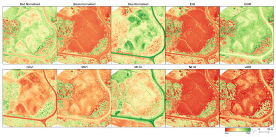
Figure A1.
False-color representation of the raster products computed from RGB bands.
Figure A1.
False-color representation of the raster products computed from RGB bands.
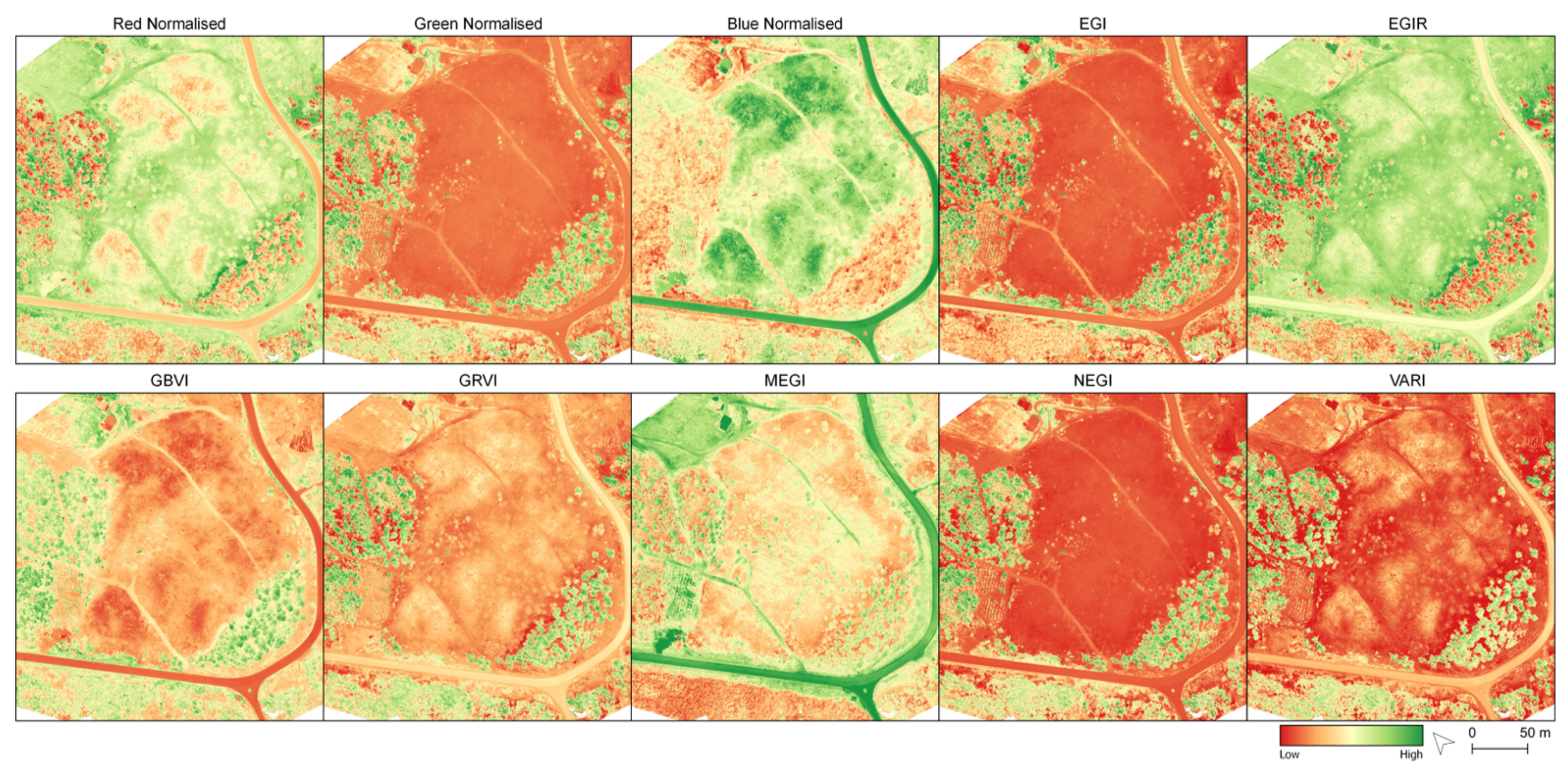
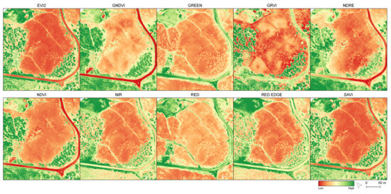
Figure A2.
False-color representation of the raster products computed from multispectral data.
Figure A2.
False-color representation of the raster products computed from multispectral data.
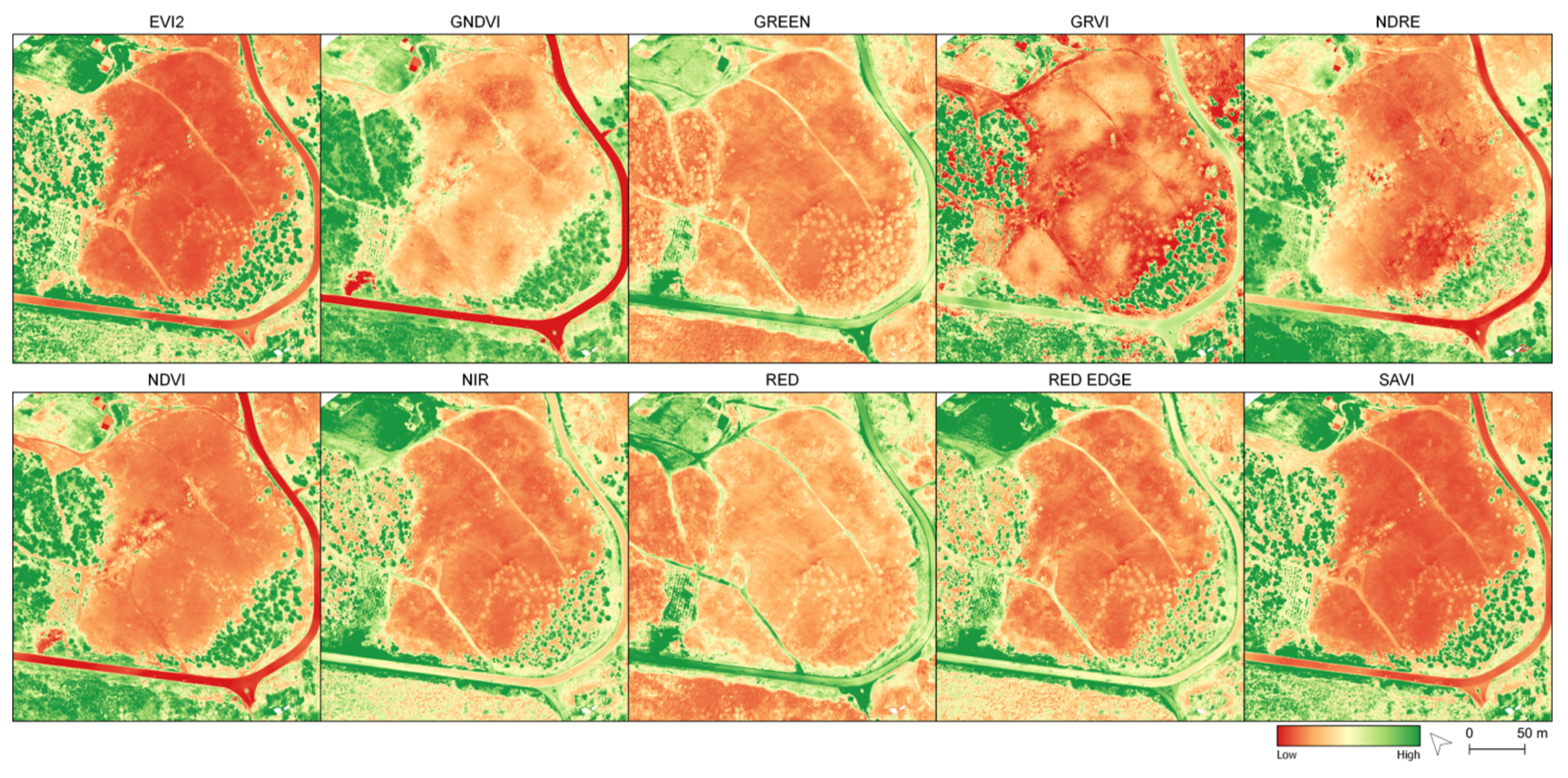
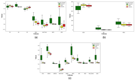
Figure A3.
Variation of the values of the RGB and multispectral indices in the three burn severity classes: (a) normalized RGB indices and bands, (b) RGB indices that are not normalized, and (c) multispectral indices and the reflectance of each band.
Figure A3.
Variation of the values of the RGB and multispectral indices in the three burn severity classes: (a) normalized RGB indices and bands, (b) RGB indices that are not normalized, and (c) multispectral indices and the reflectance of each band.
References
- FAO; UNEP. The State of the World’s Forests 2020: Forests, Biodiversity and People; FAO: Rome, Italy; UNEP: Rome, Italy, 2020; ISBN 978-92-5-132419-6. [Google Scholar]
- Oliveira, S.; Rocha, J.; Sá, A. Wildfire risk modeling. Curr. Opin. Environ. Sci. Health 2021, 23, 100274. [Google Scholar] [CrossRef]
- Mohapatra, A.; Trinh, T. Early Wildfire Detection Technologies in Practice—A Review. Sustainability 2022, 14, 12270. [Google Scholar] [CrossRef]
- Bright, B.C.; Hudak, A.T.; Kennedy, R.E.; Braaten, J.D.; Henareh Khalyani, A. Examining post-fire vegetation recovery with Landsat time series analysis in three western North American forest types. Fire Ecol. 2019, 15, 8. [Google Scholar] [CrossRef]
- Kolden, C.A.; Weisberg, P.J. Assessing accuracy of manually-mapped wildfire perimeters in topographically dissected areas. Fire Ecol. 2007, 3, 22–31. [Google Scholar] [CrossRef]
- Chuvieco, E.; Mouillot, F.; Van der Werf, G.R.; San Miguel, J.; Tanase, M.; Koutsias, N.; García, M.; Yebra, M.; Padilla, M.; Gitas, I.; et al. Historical background and current developments for mapping burned area from satellite Earth observation. Remote Sens. Environ. 2019, 225, 45–64. [Google Scholar] [CrossRef]
- Pereira, P.; Bogunovic, I.; Zhao, W.; Barcelo, D. Short-term effect of wildfires and prescribed fires on ecosystem services. Curr. Opin. Environ. Sci. Health 2021, 22, 100266. [Google Scholar] [CrossRef]
- Sanderfoot, O.; Bassing, S.; Brusa, J.; Emmet, R.; Gillman, S.; Swift, K.; Gardner, B. A review of the effects of wildfire smoke on the health and behavior of wildlife. Environ. Res. Lett. 2022, 16, 123003. [Google Scholar] [CrossRef]
- DeBano, L.F.; Neary, D.G.; Ffolliott, P.F. Fire Effects on Ecosystems; John Wiley & Sons: Hoboken, NJ, USA, 1998. [Google Scholar]
- Caon, L.; Vallejo, V.R.; Ritsema, C.J.; Geissen, V. Effects of wildfire on soil nutrients in Mediterranean ecosystems. Earth-Sci. Rev. 2014, 139, 47–58. [Google Scholar] [CrossRef]
- Albery, G.F.; Turilli, I.; Joseph, M.B.; Foley, J.; Frere, C.H.; Bansal, S. From flames to inflammation: How wildfires affect patterns of wildlife disease. Fire Ecol. 2021, 17, 1–17. [Google Scholar] [CrossRef]
- Pérez-Cabello, F.; Montorio, R.; Alves, D.B. Remote sensing techniques to assess post-fire vegetation recovery. Curr. Opin. Environ. Sci. Health 2021, 21, 100251. [Google Scholar] [CrossRef]
- Chuvieco, E.; Aguado, I.; Yebra, M.; Nieto, H.; Salas, J.; Martín, M.P.; Vilar, L.; Martínez, J.; Martín, S.; Ibarra, P.; et al. Development of a framework for fire risk assessment using remote sensing and geographic information system technologies. Ecol. Model. 2010, 221, 46–58. [Google Scholar] [CrossRef]
- Noonan-Wright, E.; Seielstad, C. Factors influencing risk during wildfires: Contrasting divergent regions in the US. Fire 2022, 5, 131. [Google Scholar] [CrossRef]
- Bergonse, R.; Oliveira, S.; Zêzere, J.L.; Moreira, F.; Ribeiro, P.F.; Leal, M.; e Santos, J.M.L. Biophysical controls over fire regime properties in Central Portugal. Sci. Total Environ. 2022, 810, 152314. [Google Scholar] [CrossRef] [PubMed]
- Liu, W.; Guan, H.; Hesp, P.A.; Batelaan, O. Remote sensing delineation of wildfire spatial extents and post-fire recovery along a semi-arid climate gradient. Ecol. Inform. 2023, 78, 102304. [Google Scholar] [CrossRef]
- Dalezios, N.R.; Kalabokidis, K.; Koutsias, N.; Vasilakos, C. Wildfires and remote sensing: An overview. In Remote Sensing of Hydrometeorological Hazards; CRC Press: Boca Raton, FL, USA, 2017; pp. 211–236. [Google Scholar]
- Kurbanov, E.; Vorobev, O.; Lezhnin, S.; Sha, J.; Wang, J.; Li, X.; Cole, J.; Dergunov, D.; Wang, Y. Remote sensing of forest burnt area, burn severity, and post-fire recovery: A review. Remote Sens. 2022, 14, 4714. [Google Scholar] [CrossRef]
- Crowley, M.A.; Stockdale, C.A.; Johnston, J.M.; Wulder, M.A.; Liu, T.; McCarty, J.L.; Rieb, J.T.; Cardille, J.A.; White, J.C. Towards a whole-system framework for wildfire monitoring using Earth observations. Glob. Chang. Biol. 2023, 29, 1423–1436. [Google Scholar] [CrossRef] [PubMed]
- Yuan, C.; Liu, Z.; Zhang, Y. Fire detection using infrared images for UAV-based forest fire surveillance. In Proceedings of the 2017 International Conference on Unmanned Aircraft Systems (ICUAS), Miami, FL, USA, 13–16 June 2017; pp. 567–572. [Google Scholar]
- Wing, M.G.; Burnett, J.D.; Sessions, J. Remote sensing and unmanned aerial system technology for monitoring and quantifying forest fire impacts. Int. J. Remote Sens. Appl. 2014, 4, 18–35. [Google Scholar] [CrossRef]
- Ollero, A.; Merino, L. Unmanned aerial vehicles as tools for forest-fire fighting. For. Ecol. Manag. 2006, 234, S263. [Google Scholar] [CrossRef]
- Szpakowski, D.M.; Jensen, J.L. A review of the applications of remote sensing in fire ecology. Remote Sens. 2019, 11, 2638. [Google Scholar] [CrossRef]
- Torresan, C.; Berton, A.; Carotenuto, F.; Di Gennaro, S.F.; Gioli, B.; Matese, A.; Miglietta, F.; Vagnoli, C.; Zaldei, A.; Wallace, L. Forestry applications of UAVs in Europe: A review. Int. J. Remote Sens. 2017, 38, 2427–2447. [Google Scholar] [CrossRef]
- Sun, Z.; Wang, X.; Wang, Z.; Yang, L.; Xie, Y.; Huang, Y. UAVs as remote sensing platforms in plant ecology: Review of applications and challenges. J. Plant Ecol. 2021, 14, 1003–1023. [Google Scholar] [CrossRef]
- Matese, A.; Toscano, P.; Di Gennaro, S.F.; Genesio, L.; Vaccari, F.P.; Primicerio, J.; Belli, C.; Zaldei, A.; Bianconi, R.; Gioli, B. Intercomparison of UAV, aircraft and satellite remote sensing platforms for precision viticulture. Remote Sens. 2015, 7, 2971–2990. [Google Scholar] [CrossRef]
- Fernández-Guisuraga, J.M.; Sanz-Ablanedo, E.; Suárez-Seoane, S.; Calvo, L. Using Unmanned Aerial Vehicles in Postfire Vegetation Survey Campaigns through Large and Heterogeneous Areas: Opportunities and Challenges. Sensors 2018, 18, 586. [Google Scholar] [CrossRef] [PubMed]
- Chuvieco, E.; Aguado, I.; Salas, J.; García, M.; Yebra, M.; Oliva, P. Satellite remote sensing contributions to wildland fire science and management. Curr. For. Rep. 2020, 6, 81–96. [Google Scholar] [CrossRef]
- Pádua, L.; Vanko, J.; Hruška, J.; Adão, T.; Sousa, J.J.; Peres, E.; Morais, R. UAS, sensors, and data processing in agroforestry: A review towards practical applications. Int. J. Remote Sens. 2017, 38, 2349–2391. [Google Scholar] [CrossRef]
- Pádua, L.; Guimarães, N.; Adão, T.; Sousa, A.; Peres, E.; Sousa, J.J. Effectiveness of Sentinel-2 in Multi-Temporal Post-Fire Monitoring When Compared with UAV Imagery. ISPRS Int. J. Geo-Inf. 2020, 9, 225. [Google Scholar] [CrossRef]
- Dainelli, R.; Toscano, P.; Di Gennaro, S.F.; Matese, A. Recent advances in unmanned aerial vehicle forest remote sensing—A systematic review. Part I: A general framework. Forests 2021, 12, 327. [Google Scholar] [CrossRef]
- Mohsan, S.A.H.; Othman, N.Q.H.; Li, Y.; Alsharif, M.H.; Khan, M.A. Unmanned aerial vehicles (UAVs): Practical aspects, applications, open challenges, security issues, and future trends. Intell. Serv. Robot. 2023, 16, 109–137. [Google Scholar] [CrossRef]
- Koutsias, N.; Karteris, M.; Chuvico, E. The use of intensity-hue-saturation transformation of Landsat-5 Thematic Mapper data for burned land mapping. Photogramm. Eng. Remote Sens. 2000, 66, 829–840. [Google Scholar]
- McKenna, P.; Erskine, P.D.; Lechner, A.M.; Phinn, S. Measuring fire severity using UAV imagery in semi-arid central Queensland, Australia. Int. J. Remote Sens. 2017, 38, 4244–4264. [Google Scholar] [CrossRef]
- Deshpande, M.V.; Pillai, D.; Jain, M. Agricultural burned area detection using an integrated approach utilizing multi spectral instrument based fire and vegetation indices from Sentinel-2 satellite. MethodsX 2022, 9, 101741. [Google Scholar] [CrossRef] [PubMed]
- Rouse, J.W.; Haas, R.H.; Schell, J.A.; Deering, D.W. Monitoring vegetation systems in the Great Plains with ERTS. NASA Spec. Publ. 1974, 351, 309–317. [Google Scholar]
- Key, C.; Benson, N. Landscape Assessment: Ground measure of severity, the Composite Burn Index and Remote sensing of severity, the Normalized Burn Ratio. In FIREMON: Fire Effects Monitoring and Inventory System; USDA Forest Service, Rocky Mountain Research Station: Ogden, UT, USA, 2006; p. LA 1-51. [Google Scholar]
- Chuvieco, E.; Lizundia-Loiola, J.; Pettinari, M.L.; Ramo, R.; Padilla, M.; Tansey, K.; Mouillot, F.; Laurent, P.; Storm, T.; Heil, A.; et al. Generation and analysis of a new global burned area product based on MODIS 250 m reflectance bands and thermal anomalies. Earth Syst. Sci. Data 2018, 10, 2015–2031. [Google Scholar] [CrossRef]
- Long, T.; Zhang, Z.; He, G.; Jiao, W.; Tang, C.; Wu, B.; Zhang, X.; Wang, G.; Yin, R. 30 m resolution global annual burned area mapping based on landsat images and Google Earth Engine. Remote Sens. 2019, 11, 489. [Google Scholar] [CrossRef]
- García-Llamas, P.; Suárez-Seoane, S.; Taboada, A.; Fernández-Manso, A.; Quintano, C.; Fernández-García, V.; Fernández-Guisuraga, J.M.; Marcos, E.; Calvo, L. Environmental drivers of fire severity in extreme fire events that affect Mediterranean pine forest ecosystems. For. Ecol. Manag. 2019, 433, 24–32. [Google Scholar] [CrossRef]
- Gibson, R.; Danaher, T.; Hehir, W.; Collins, L. A remote sensing approach to mapping fire severity in south-eastern Australia using sentinel 2 and random forest. Remote Sens. Environ. 2020, 240, 111702. [Google Scholar] [CrossRef]
- Collins, L.; Griffioen, P.; Newell, G.; Mellor, A. The utility of Random Forests for wildfire severity mapping. Remote Sens. Environ. 2018, 216, 374–384. [Google Scholar] [CrossRef]
- Petropoulos, G.P.; Kontoes, C.; Keramitsoglou, I. Burnt area delineation from a uni-temporal perspective based on landsat TM imagery classification using Support Vector Machines. Int. J. Appl. Earth Obs. Geoinf. 2011, 13, 70–80. [Google Scholar] [CrossRef]
- Gómez, I.; Martín, M.P. Prototyping an artificial neural network for burned area mapping on a regional scale in Mediterranean areas using MODIS images. Int. J. Appl. Earth Obs. Geoinf. 2011, 13, 741–752. [Google Scholar] [CrossRef]
- Sedano, F.; Kempeneers, P.; Strobl, P.; McInerney, D.; Miguel, J.S. Increasing Spatial Detail of Burned Scar Maps Using IRS-AWiFS Data for Mediterranean Europe. Remote Sens. 2012, 4, 726–744. [Google Scholar] [CrossRef]
- Seydi, S.T.; Hasanlou, M.; Chanussot, J. Burnt-Net: Wildfire burned area mapping with single post-fire Sentinel-2 data and deep learning morphological neural network. Ecol. Indic. 2022, 140, 108999. [Google Scholar] [CrossRef]
- Guindos-Rojas, F.; Arbelo, M.; García-Lázaro, J.R.; Moreno-Ruiz, J.A.; Hernández-Leal, P.A. Evaluation of a Bayesian algorithm to detect Burned Areas in the Canary Islands’ Dry Woodlands and forests ecoregion using MODIS data. Remote Sens. 2018, 10, 789. [Google Scholar] [CrossRef]
- García-Lázaro, J.R.; Moreno-Ruiz, J.A.; Riaño, D.; Arbelo, M. Estimation of burned area in the Northeastern Siberian boreal forest from a Long-Term Data Record (LTDR) 1982–2015 time series. Remote Sens. 2018, 10, 940. [Google Scholar] [CrossRef]
- Ruiz, J.A.M.; Lázaro, J.R.G.; Águila Cano, I.D.; Leal, P.H. Burned area mapping in the North American boreal forest using terra-MODIS LTDR (2001–2011): A comparison with the MCD45A1, MCD64A1 and BA GEOLAND-2 products. Remote Sens. 2013, 6, 815–840. [Google Scholar] [CrossRef]
- United Nations. Step by Step: Burn Severity Mapping in Google Earth Engine. Available online: https://un-spider.org/advisory-support/recommended-practices/recommended-practice-burn-severity/burn-severity-earth-engine (accessed on 15 March 2023).
- Martinez, J.L.; Lucas-Borja, M.E.; Plaza-Alvarez, P.A.; Denisi, P.; Moreno, M.A.; Hernández, D.; González-Romero, J.; Zema, D.A. Comparison of satellite and drone-based images at two spatial scales to evaluate vegetation regeneration after post-fire treatments in a mediterranean forest. Appl. Sci. 2021, 11, 5423. [Google Scholar] [CrossRef]
- Larrinaga, A.R.; Brotons, L. Greenness indices from a low-cost UAV imagery as tools for monitoring post-fire forest recovery. Drones 2019, 3, 6. [Google Scholar] [CrossRef]
- Chen, J.; Yi, S.; Qin, Y.; Wang, X. Improving estimates of fractional vegetation cover based on UAV in alpine grassland on the Qinghai–Tibetan Plateau. Int. J. Remote Sens. 2016, 37, 1922–1936. [Google Scholar] [CrossRef]
- Gobron, N.; Pinty, B.; Verstraete, M.M.; Widlowski, J.L. Advanced vegetation indices optimized for up-coming sensors: Design, performance, and applications. IEEE Trans. Geosci. Remote. Sens. 2000, 38, 2489–2505. [Google Scholar]
- Hunt, E.R., Jr.; Daughtry, C.; Eitel, J.U.; Long, D.S. Remote sensing leaf chlorophyll content using a visible band index. Agron. J. 2011, 103, 1090–1099. [Google Scholar] [CrossRef]
- Tucker, C.J. Red and photographic infrared linear combinations for monitoring vegetation. Remote Sens. Environ. 1979, 8, 127–150. [Google Scholar] [CrossRef]
- Kawashima, S.; Nakatani, M. An algorithm for estimating chlorophyll content in leaves using a video camera. Ann. Bot. 1998, 81, 49–54. [Google Scholar] [CrossRef]
- Gitelson, A.A.; Kaufman, Y.J.; Stark, R.; Rundquist, D. Novel algorithms for remote estimation of vegetation fraction. Remote Sens. Environ. 2002, 80, 76–87. [Google Scholar] [CrossRef]
- Jiang, Z.; Huete, A.R.; Didan, K.; Miura, T. Development of a two-band enhanced vegetation index without a blue band. Remote Sens. Environ. 2008, 112, 3833–3845. [Google Scholar] [CrossRef]
- Gitelson, A.A.; Kaufman, Y.J.; Merzlyak, M.N. Use of a green channel in remote sensing of global vegetation from EOS-MODIS. Remote Sens. Environ. 1996, 58, 289–298. [Google Scholar] [CrossRef]
- Gitelson, A.; Merzlyak, M.N. Spectral reflectance changes associated with autumn senescence of Aesculus hippocastanum L. and Acer platanoides L. leaves. Spectral features and relation to chlorophyll estimation. J. Plant Physiol. 1994, 143, 286–292. [Google Scholar] [CrossRef]
- Huete, A.R. A soil-adjusted vegetation index (SAVI). Remote Sens. Environ. 1988, 25, 295–309. [Google Scholar] [CrossRef]
- Inglada, J.; Christophe, E. The Orfeo Toolbox remote sensing image processing software. In Proceedings of the 2009 IEEE International Geoscience and Remote Sensing Symposium, Cape Town, South Africa, 12–17 July 2009; Volume 4. [Google Scholar]
- Bradski, G. The OpenCV Library. Dr. Dobb’s J. Softw. Tools 2000, 25, 120–123. [Google Scholar]
- Chang, C.C.; Lin, C.J. LIBSVM: A library for support vector machines. ACM Trans. Intell. Syst. Technol. (TIST) 2011, 2, 1–27. [Google Scholar] [CrossRef]
- Pedregosa, F.; Varoquaux, G.; Gramfort, A.; Michel, V.; Thirion, B.; Grisel, O.; Blondel, M.; Prettenhofer, P.; Weiss, R.; Dubourg, V.; et al. Scikit-learn: Machine Learning in Python. J. Mach. Learn. Res. 2011, 12, 2825–2830. [Google Scholar]
- Pérez-Rodríguez, L.A.; Quintano, C.; Marcos, E.; Suarez-Seoane, S.; Calvo, L.; Fernández-Manso, A. Evaluation of Prescribed Fires from Unmanned Aerial Vehicles (UAVs) Imagery and Machine Learning Algorithms. Remote Sens. 2020, 12, 1295. [Google Scholar] [CrossRef]
- Arnett, J.T.; Coops, N.C.; Daniels, L.D.; Falls, R.W. Detecting forest damage after a low-severity fire using remote sensing at multiple scales. Int. J. Appl. Earth Obs. Geoinf. 2015, 35, 239–246. [Google Scholar] [CrossRef]
- Adugna, T.; Xu, W.; Fan, J. Comparison of random forest and support vector machine classifiers for regional land cover mapping using coarse resolution FY-3C images. Remote Sens. 2022, 14, 574. [Google Scholar] [CrossRef]
- Liu, M.; Wang, M.; Wang, J.; Li, D. Comparison of random forest, support vector machine and back propagation neural network for electronic tongue data classification: Application to the recognition of orange beverage and Chinese vinegar. Sens. Actuators B Chem. 2013, 177, 970–980. [Google Scholar] [CrossRef]
- Shamsoshoara, A.; Afghah, F.; Razi, A.; Zheng, L.; Fulé, P.Z.; Blasch, E. Aerial imagery pile burn detection using deep learning: The FLAME dataset. Comput. Netw. 2021, 193, 108001. [Google Scholar] [CrossRef]
- Ghali, R.; Akhloufi, M.A.; Mseddi, W.S. Deep learning and transformer approaches for UAV-based wildfire detection and segmentation. Sensors 2022, 22, 1977. [Google Scholar] [CrossRef]
- Yuan, C.; Liu, Z.; Zhang, Y. Aerial images-based forest fire detection for firefighting using optical remote sensing techniques and unmanned aerial vehicles. J. Intell. Robot. Syst. 2017, 88, 635–654. [Google Scholar] [CrossRef]
- Jiao, Z.; Zhang, Y.; Xin, J.; Mu, L.; Yi, Y.; Liu, H.; Liu, D. A deep learning based forest fire detection approach using UAV and YOLOv3. In Proceedings of the 2019 1st International Conference on Industrial Artificial Intelligence (IAI), Shenyang, China, 23–27 July 2019; pp. 1–5. [Google Scholar]
- Hendel, I.G.; Ross, G.M. Efficacy of remote sensing in early forest fire detection: A thermal sensor comparison. Can. J. Remote Sens. 2020, 46, 414–428. [Google Scholar] [CrossRef]
- Deligiannakis, G.; Pallikarakis, A.; Papanikolaou, I.; Alexiou, S.; Reicherter, K. Detecting and monitoring early post-fire sliding phenomena using UAV–SfM photogrammetry and t-LiDAR-derived point clouds. Fire 2021, 4, 87. [Google Scholar] [CrossRef]
- van Blerk, J.; West, A.; Smit, J.; Altwegg, R.; Hoffman, M. UAVs improve detection of seasonal growth responses during post-fire shrubland recovery. Landsc. Ecol. 2022, 37, 3179–3199. [Google Scholar] [CrossRef]
- Qarallah, B.; Al-Ajlouni, M.; Al-Awasi, A.; Alkarmy, M.; Al-Qudah, E.; Naser, A.B.; Al-Assaf, A.; Gevaert, C.M.; Al Asmar, Y.; Belgiu, M.; et al. Evaluating post-fire recovery of Latroon dry forest using Landsat ETM+, unmanned aerial vehicle and field survey data. J. Arid. Environ. 2021, 193, 104587. [Google Scholar] [CrossRef]
- Fernández-Guisuraga, J.M.; Calvo, L.; Suarez-Seoane, S. Monitoring post-fire neighborhood competition effects on pine saplings under different environmental conditions by means of UAV multispectral data and structure-from-motion photogrammetry. J. Environ. Manag. 2022, 305, 114373. [Google Scholar] [CrossRef] [PubMed]
- Mohan, M.; Richardson, G.; Gopan, G.; Aghai, M.M.; Bajaj, S.; Galgamuwa, G.P.; Vastaranta, M.; Arachchige, P.S.P.; Amorós, L.; Corte, A.P.D.; et al. UAV-supported forest regeneration: Current trends, challenges and implications. Remote Sens. 2021, 13, 2596. [Google Scholar] [CrossRef]
- Bayer, A.P.A. Biomass Forest Modelling Using UAV LiDAR Data under Fire Effect. Master’s Thesis, Universidade de Lisboa, Lisbon, Portugal, 2019. [Google Scholar]
- Shrestha, M.; Broadbent, E.N.; Vogel, J.G. Using GatorEye UAV-Borne LiDAR to Quantify the Spatial and Temporal Effects of a Prescribed Fire on Understory Height and Biomass in a Pine Savanna. Forests 2020, 12, 38. [Google Scholar] [CrossRef]
- Carvajal-Ramírez, F.; da Silva, J.R.M.; Agüera-Vega, F.; Martínez-Carricondo, P.; Serrano, J.; Moral, F.J. Evaluation of fire severity indices based on pre- and post-fire multispectral imagery sensed from UAV. Remote Sens. 2019, 11, 993. [Google Scholar] [CrossRef]
Disclaimer/Publisher’s Note: The statements, opinions and data contained in all publications are solely those of the individual author(s) and contributor(s) and not of MDPI and/or the editor(s). MDPI and/or the editor(s) disclaim responsibility for any injury to people or property resulting from any ideas, methods, instructions or products referred to in the content. |
© 2023 by the authors. Licensee MDPI, Basel, Switzerland. This article is an open access article distributed under the terms and conditions of the Creative Commons Attribution (CC BY) license (https://creativecommons.org/licenses/by/4.0/).