Radar Emitter Signal Intra-Pulse Modulation Open Set Recognition Based on Deep Neural Network

Abstract

Radar emitter signal intra-pulse modulation recognition is important for modern electronic reconnaissance systems to analyze target radar systems. In the actual environment, the intra-pulse modulations of the sampled radar emitter signals contain not only the known types in the library but also the unknown types. Therefore, the existing recognition methods, which are based on a closed set, cannot recognize the unknown samples. In order to solve this problem, in this paper, we proposed a method for radar emitter signal intra-pulse modulation open set recognition. The proposed method could classify the known modulations and identify the unknown modulation by using an original deep neural network-based recognition model trained on a closed set, estimating the signal-to-noise ratio, and calculating the reconstruction loss by an encoder–decoder model. For a given sample, the original deep neural network-based recognition model will label it as a certain known class temporarily. By estimating the SNR of the sample and calculating the reconstruction loss by inputting the sample to the corresponding encoder–decoder model related to the temporary predicted known class, whether the sample belongs to the predicted temporary known class or the unknown class will be confirmed. Experiments were conducted with five different openness conditions. The experimental results indicate that the proposed method has good performance on radar emitter signal intra-pulse modulation open set recognition.

1. Introduction

The modern electromagnetic environment has become more complex with the advancement of modern radar systems [1], and the number of types of intra-pulse modulation of radar emitter signals is increasing. Intra-pulse modulation recognition technologies are important for modern electronic reconnaissance systems, such as electronic support measure (ESM) systems, electronic intelligence (ELINT) systems, and radar warning receivers (RWRs) [2,3,4]. Accurately recognizing the intra-pulse modulation of radar emitter signals could increase the reliability of analyzing the function and information of the target radar.

Due to the rapid development of deep learning, recently, many researchers have combined deep learning methods and radar technologies to recognize intra-pulse modulations of radar emitter signals. In [5], Qu et al. preprocessed time-domain signals to obtain time-frequency images (TFIs) by using a Cohen class time-frequency distribution. Then, they designed a convolutional neural network (CNN) to recognize the intra-pulse modulations. In [6], Yu et al. used short-time Fourier transformation (STFT) to convert radar signals into TFIs, and then trained a CNN model to recognize their intra-pulse modulation. In [7], Yuan et al. proposed a 1-D selective kernel convolutional neural network to recognize eleven types of intra-pulse modulations based on the frequency-domain sequences of radar emitter signals. Wu et al. [8] combined a 1-D CNN and attention mechanism to recognize seven types of radar emitter signal intra-pulse modulations in the time domain. Si et al. [9] used a smooth pseudo-Wigner–Ville distribution transformation to covert dual-component radar signals in the time domain into TFIs and accomplished multi-label recognition tasks by using EfficientNet [10]. Similarly, Wan et al. [11] proposed a novel modulation recognition method of multi-component radar signals based on the deep convolutional neural network with a convolutional block attention module (DCNN-CBAM) to recognize multi-component radar signals. In [12], Cai et al. proposed a self-supervised learning framework with virtual adversarial training, which overcomes the limitation that the performance of radar signal intra-pulse modulation recognition mainly relies on a large number of labeled samples. Unlike most of the fully supervised situations, Yuan et al. [13] focused on a more common situation, where a very limited number of labeled samples and a large number of unlabeled samples are provided, and proposed a semi-supervised intra-pulse modulation recognition method.

However, there are still some problems in the above intra-pulse modulation recognition methods. The existing intra-pulse modulation recognition methods focus on the situation that the types of intra-pulse modulation in the testing dataset are the same types of intra-pulse modulation in the training dataset. Therefore, this type of intra-pulse modulation recognition is closed set recognition (CSR). Based on this assumption, these deep neural network-based methods perform well. But in the real environment, intra-pulse modulations are varied. Except for the known intra-pulse modulation types, unknown types emerge from time to time. These existing deep neural network-based CSR methods will naturally but mistakenly recognize an unknown type of intra-pulse modulation as one of the known types. Although the occurrence probability of this situation could be reduced by collecting as many types of intra-pulse modulations as possible, their collection for a training library is difficult as intra-pulse modulations are mainly used in the military field. In practical applications, it is important to not only classify the known classes but also label the unknown classes, which is called open set recognition (OSR). The OSR of radar emitter signal intra-pulse modulations is a tough challenge of great significance for the analysis of the information of a target radar emitter.

Recently, OSR methods have been shifted to the deep learning field. In [14], Hendrycks et al. presented a method using softmax distributions to detect misclassified and out-of-distribution samples, which provides the possibility of OSR in a deep neural network (DNN). The most representative research is that of Bendale et al. [15], who proposed the OpenMax approach based on the theory of the Weibull distribution, which replaced the softmax layer with an OpenMax layer to reassign the value of the activation vector. In the field of radar signal recognition, many studies have been conducted. For example, in [16], Sun et al. proposed a pseudo-signal generation and recognition neural network to identify specific emitters under an open set condition. Zhou et al. [17] presented two models for radar jamming OSR that can accurately classify known jamming and distinguish unknown jamming.

With increasingly complex electromagnetic environments, intra-pulse modulation recognition methods should be able to deal with an open set condition. These methods should not only classify the known intra-pulse modulations with high accuracy, but also have the ability to identify the unknown intra-pulse modulations correctly. Due to the great success of DNN-based methods in radar emitter signal intra-pulse modulation recognition, we proposed a DNN-based method to solve the OSR problem in intra-pulse modulation. This method does not change the existing well-trained recognition model in a closed set condition. Instead, in this method, taking the number of known intra-pulse modulations, we design the same number of encoder–decoder models to reconstruct the TFIs in the same class through compression and decompression. By estimating the signal-to-noise ratio (SNR) for each sample in a validation dataset, using the corresponding encoder–decoder model to calculate the reconstruction loss for the samples in the validation dataset, the thresholds with SNR for classifying known and unknown intra-pulse modulation could be set based on different recognition accuracies of the known classes. Combined the recognition results from the existing well-trained recognition model with the SNR of the testing samples, thresholds with SNR, and reconstruction loss values, the original recognition result could be revised.

The main contribution of this paper is that unlike most of the closed set situations, we focus on a more common open set situation, where the unknown samples are included for recognition during the testing session. Another contribution is that our method is based on the DNN with a closed set situation, which is trained only with known samples. Through estimating the SNR and calculating the reconstruction loss for testing the sample based on the proposed encoder–decoder model, the recognition result could be confirmed as a certain known class or as an unknown class.

This paper is organized as follows: In Section 2, the proposed method is described in detail. The dataset and experimental settings are shown in Section 3. The extensive experiments and corresponding analysis are described in Section 4. The ablation study is given in Section 5. Finally, the conclusion is presented in Section 6.

2. Materials and Methods

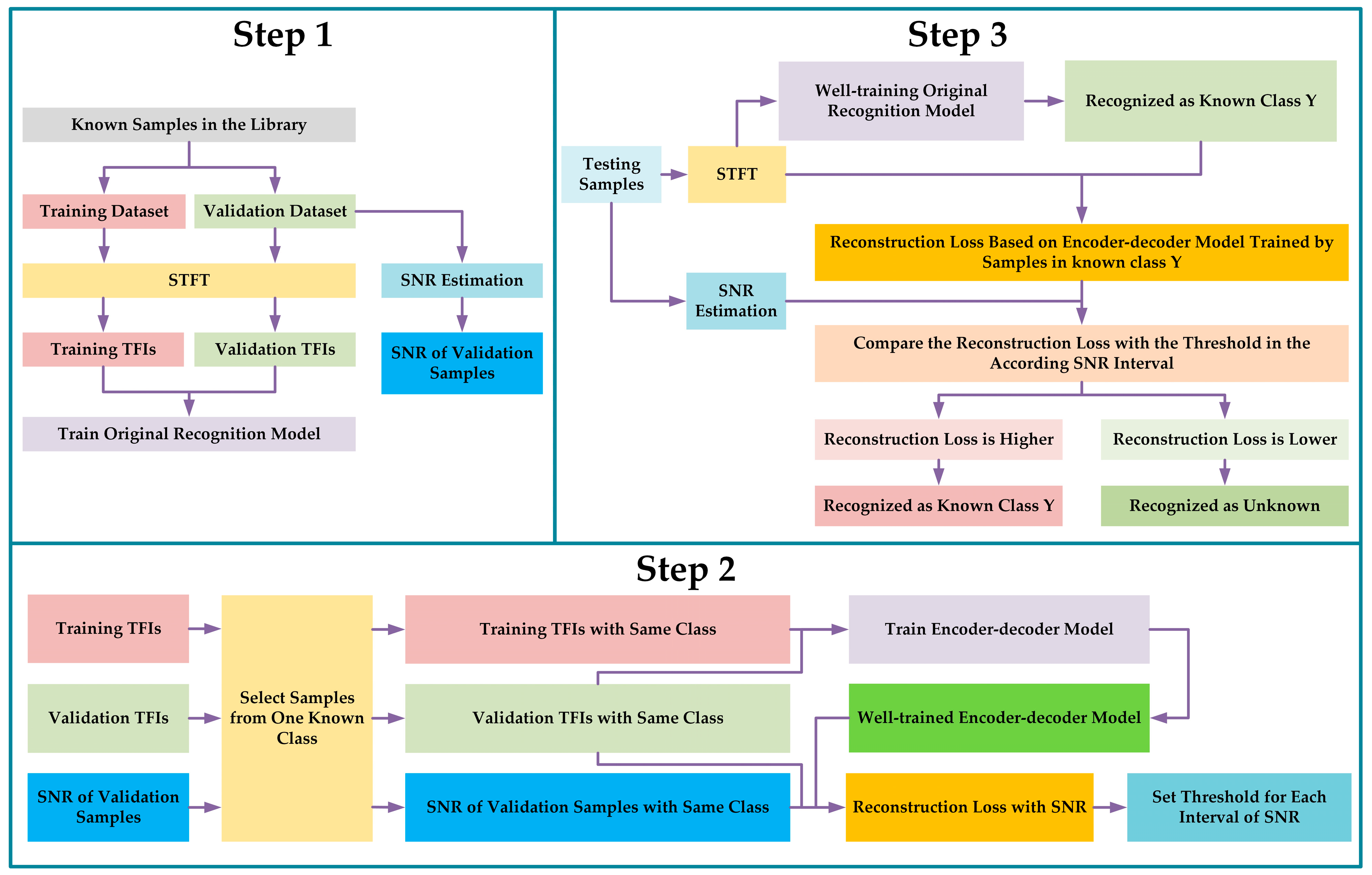
OSR of intra-pulse modulation refers to a case in which the samples used for the training model are in a certain number of classes. When the model is applied for a testing session, the types of intra-pulse modulation for the testing samples not only include the known classes from the training library, but also the unknown classes.

Let $X_{train}=\left\{(x_i,y_i):i\in (1,2,\dots ,K_{train})\right\}$ be a known dataset in the library, where $x_i$ and $y_i$ are the known samples and the corresponding labels, and $K_{train}$ is the number of total samples. The label of $y_i$ belongs to $\{1,2,\dots ,N\}$, where $N$ is the number of total known classes. For the testing dataset $X_{test}=\left\{(x_j^{test},y_j^{test}):j\in (1,2,\dots ,K_{test})\right\}$, where $x_j^{test}$ and $y_j^{test}$ are the testing samples and the corresponding labels, and $K_{test}$ is the number of total samples. In this case, the label of $y_j^{test}$ belongs to $\{1,2,\dots ,N,N+1\}$, where the category of $\{1,2,\dots ,N\}$ refers to the known classes and the category of $\{N+1\}$ refers to the unknown class. Therefore, a good model for intra-pulse modulation OSR should have good accuracy not only in classifying samples from known classes, but also in identifying samples from unknown classes.

In this paper, the method for intra-pulse modulation OSR mainly consists of 3 steps:

Step 1: Data preprocessing and original recognition model training.

(1)

Split the known samples dataset into a training dataset and validation dataset. Note that both the training dataset and validation dataset do not contain unknown samples.

(2)

Estimate the SNR for each sample in the validation dataset.

(3)

Convert the training samples and validation samples into TFIs by using STFT.

(4)

Train an original recognition model in the CSR way with TFIs.

Step 2: Encoder–decoder model training and threshold setting.

(1)

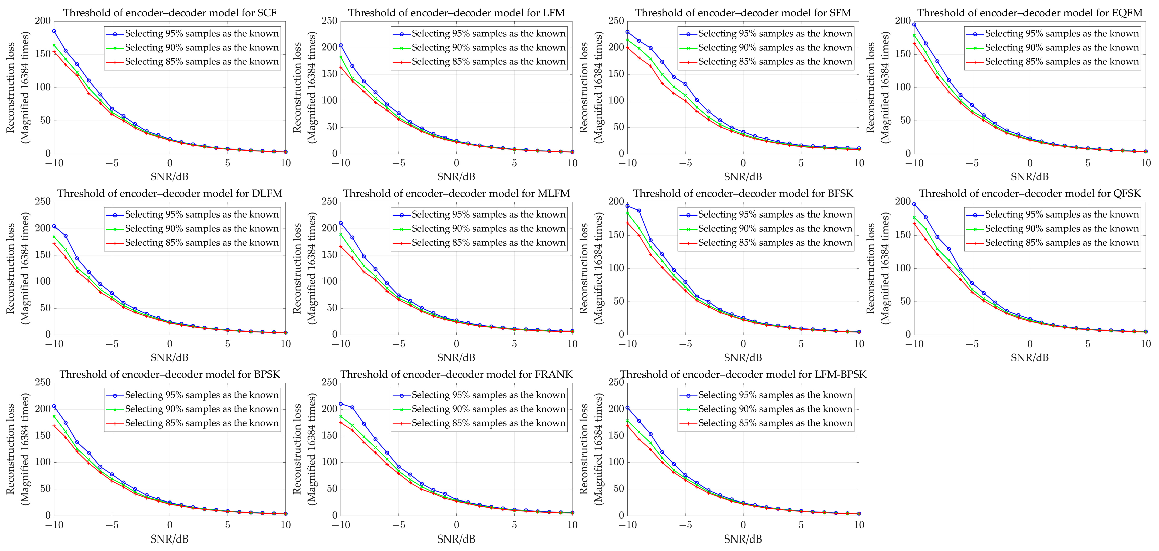
Select the samples from one known class and only use these TFIs to train the encoder–decoder model. Then, use the corresponding encoder–decoder model to calculate the reconstruction loss of the corresponding validation TFIs. As the SNR of the validation samples has been obtained, by setting the interval of SNR, the corresponding reconstruction loss in each interval of SNR could be counted. In this paper, the reconstruction loss is mean square error (MSE). Note that the number of encoder–decoder models is the same as the number of known classes. For example, if there are 11 known classes, then there will be 11 corresponding encoder–decoder models, where each model is only responsible for reconstructing one class.

(2)

Set the threshold for reconstruction loss in each interval of SNR. The details of the threshold setting are introduced as follows: For a known class, we could calculate the reconstruction loss of its validation samples from each SNR interval. Assuming that each SNR interval contains 400 samples, for example, then, we sort these 400 samples’ reconstruction losses from a low value to a high value for each interval. Then we set, for example, the top highest 1%, 2%, …, 25%, etc. reconstruction losses of these 400 samples as the threshold. Similarly, we could get the thresholds for the other known classes based on the above operation. Note that the ratio (1%, 2%, …, 25%, etc.) is the same for each SNR interval in each known class. After obtaining all of the thresholds for each SNR interval of all of the known classes, we could evaluate the recognition accuracy in the validation dataset through the corresponding thresholds controlled by the same ratio (like 5%). For example, if we set the ratio as 5%, that means the corresponding threshold will be related to the top 5% highest reconstruction losses in each SNR interval for each known class in the validation dataset. Based on the ratio, the recognition results will be revised (some samples will be labeled as unknown), leading to different mean recognition accuracies in the known class validation dataset. Therefore, by setting a suitable ratio, it could be ensured that the methods have 80%, 85%, 90%, and 95%, respectively, mean recognition accuracy (also the mean recognition accuracy for known classes) on the corresponding validation dataset. For example, when we set the ratios as 4% and 20%, the mean recognition accuracies on the validation dataset are 95% and 80%, respectively. Based on this threshold setting with 80%, 85%, 90%, and 95% mean recognition accuracy on the validation dataset, we test the methods with the corresponding testing dataset.

(3)

Perform (1) and (2) in Step 2 until all of the known classes are covered.

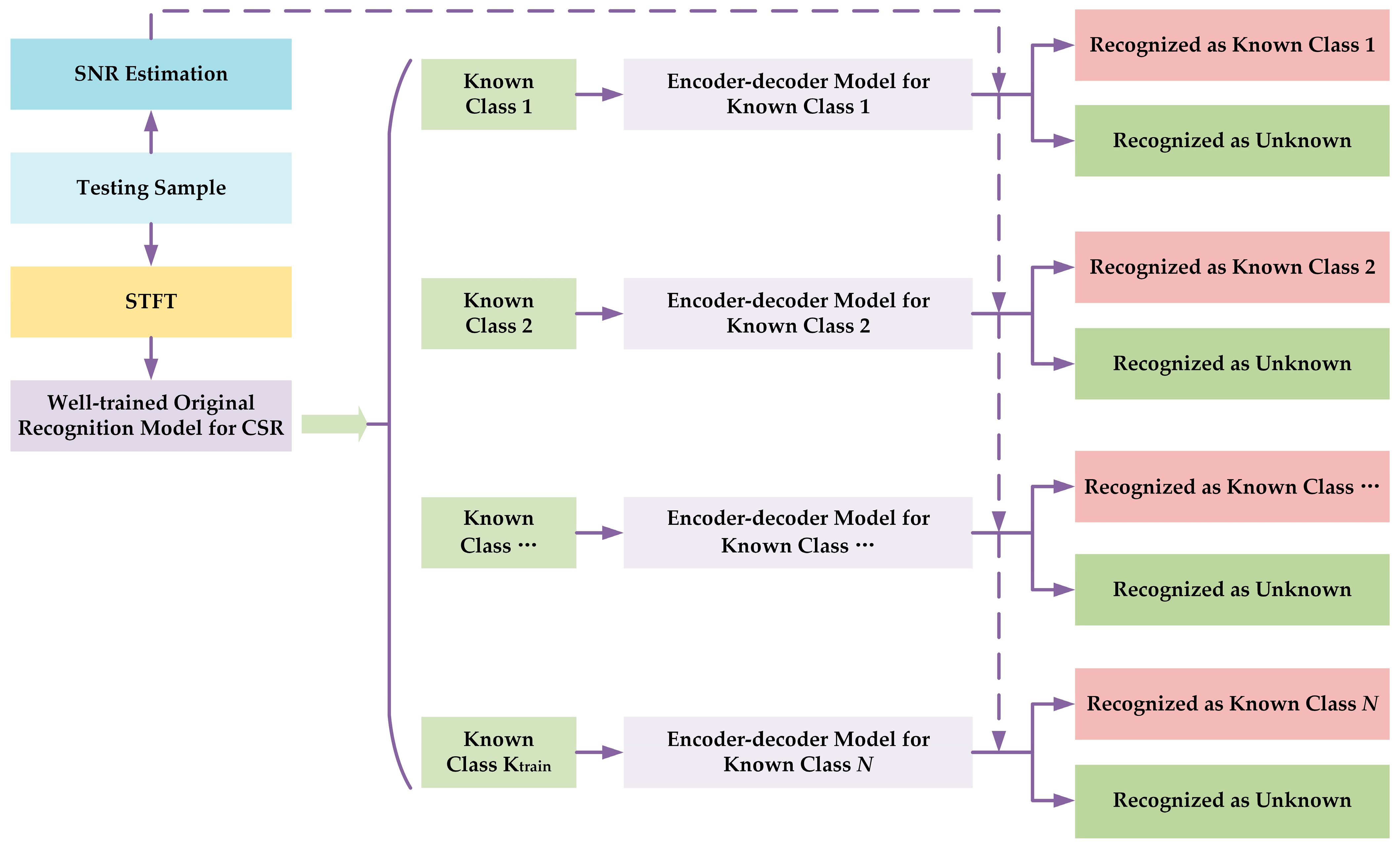
Step 3: Recognition of the testing sample.

(1)

Estimate the SNR for the testing samples and convert the testing samples to TFIs by using STFT. Now the testing samples contain the unknown class.

(2)

Use the well-trained recognition model in Step 1 to predict the class of the testing sample.

(3)

Based on the prediction result, use the corresponding encoder–decoder model to calculate the reconstruction loss of this testing sample. For example, if a testing sample is recognized as category $\left\{2\right\}$, then only the encoder–decoder model for category $\left\{2\right\}$ will be used to calculate its reconstruction loss.

(4)

Based on the SNR and reconstruction loss of the testing sample and the threshold for reconstruction loss in each interval of the SNR for the used encoder–decoder model, the final recognition result for this sample will be obtained. Note that if the reconstruction loss is higher than the threshold, then the corresponding sample is seen as the unknown class. If it is not, the corresponding sample is seen as the known class, and its label is the predicted result from the original recognition model.

A flow chart of the proposed intra-pulse modulation OSR method is shown in Figure 1. Figure 2 shows a sketch map of the proposed method in actual deployment.

2.1. Data Preprocessing

In this paper, we chose to use short-time Fourier transformation (STFT) to convert the time domain signal into a time-frequency domain. STFT is based on Fourier transformation, which is faster than other time-frequency analysis tools. The mathematical expression of STFT [18,19] could be written as:

$$TF(m,n)={\displaystyle \sum _{k=0}^{N-1}s(k)h(k-m)e^{-j\frac{2\pi n}{N}k}}$$

(1)

where $TF$ is the result of the STFT. $m$ and $n$ are the time index and frequency index of $TF$, respectively. $s(k)$ is the sampled sequence of the intra-pulse signal. $h(k)$ is the window function, which is used to obtain the sub-signal of $s(k)$. In this paper, the length of the obtained sub-signal $s(k)h(k-m)$ is set to be 256, which is also the value of $N$. Hamming Window is chosen as the window function, with a length of 64 (a quarter of the length of the sub-signal). Compared with a traditional Fourier transformation, which provides only global frequency-domain features, the time shift and frequency shift of the window function provide STFT with localization characteristics. By using STFT, the radar emitter signals could be analyzed with time-frequency features.

As the result of STFT is a complex matrix, first we calculate the square of the modulus value of each element in $TF$, then we resize the resulting matrix in an image processing way, where the resized result is a $128\times 128$ matrix. Finally, we normalize the value of each element in this matrix so that the value for each element of the resized matrix will range from 0 to 1. The process could be written as:

$$T{F}_{square}(a,b)=T{F}_{square}(a,b)\times T{F}_{square}^{*}(a,b),a\in [1,2,\dots ,m],b\in [1,2,\dots ,256]$$

(2)

$$\mathrm{imresize}(\cdot ):T{F}_{square}\in {ℝ}^{m\times 256}\to T{F}_{resize}\in {ℝ}^{128\times 128}$$

(3)

$$TFI(i,j)=\frac{T{F}_{resize}(i,j)-\min (T{F}_{resize})}{\max (T{F}_{resize})-\min (T{F}_{resize})},i\in [1,2,\dots ,128],j\in [1,2,\dots ,128]$$

(4)

where $T{F}_{square}$ is the result calculated by squaring each element in $TF$ and $T{F}_{square}^{*}(a,b)$ is the conjugation of $T{F}_{square}(a,b)$. The operation of $\mathrm{imresize}(\cdot )$ is based on nearest-neighbor interpolation. $T{F}_{resize}$ is the result of resizing $T{F}_{square}$ as a $128\times 128$ matrix. $\max (\cdot )$ and $\min (\cdot )$ are the functions used to obtain the max value and min value of the matrix, respectively. $TFI$ is the final result used for training and testing the model.

The results of data preprocessing based on STFT are shown in Section 3. Through the data preprocessing based on STFT, the time-domain sampled radar emitter signals with different intra-pulse modulations can be converted into time-frequency images, which are used as the input for deep neural network models.

2.2. SNR Estimation

The signal-to-noise ratio (SNR) is important for intra-pulse modulation recognition. We assume that the noise is additional white Gaussian noise [20]. Traditionally, except for the intra-pulse part, the sampler also samples the blank part, which only includes the noise. Let the received sequence of the blank part be $nois{e}_b(n)$. If the received sequence of pure intra-pulse signal is $s(n)$, then the actual received sequence of the intra-pulse signal polluted by noise could be written as:

$$x(n)=s(n)+nois{e}_{in}(n)$$

(5)

where $x(n)$ is the sampled intra-pulse sequence polluted by noise. $nois{e}_{in}(n)$ refers to the noise sequence in the intra-pulse part. The power of $x(n)$ could be calculated as follows:

$$P_x=\frac{{\displaystyle \sum _{i=0}^{N-1}{(x(i))}^2}}{N}$$

(6)

where $P_x$ is the power of $x(n)$ and $N$ is the length of the sequence in the intra-pulse part. As $P_x$ is the additional result of the power of $s(n)$ and the power of $nois{e}_{in}(n)$, the following relationship can be written as:

$$P_x=P_s+P_{nois{e}_{in}}$$

(7)

$$P_s=\frac{{\displaystyle \sum _{i=0}^{N-1}{(s(i))}^2}}{N}$$

(8)

$$P_{nois{e}_{in}}=\frac{{\displaystyle \sum _{i=0}^{N-1}{(nois{e}_{in}(i))}^2}}{N}$$

(9)

where $P_s$ and $P_{nois{e}_{in}}$ are the power of $s(n)$ and $nois{e}_{in}(n)$, respectively.

Based on the definition of SNR, the actual value of SNR is calculated as:

$$SN{R}_{actual}=10{\log }_{10}\left(\frac{P_s}{P_{nois{e}_{in}}}\right)$$

(10)

As the power of noise is stable during a period of time, the power of $n_{in}(t)$ is closely similar to that of $n_b(t)$. Therefore, the estimated SNR could be written as:

$$SN{R}_{estimated}=10{\log }_{10}\left(\frac{P_x-P_{nois{e}_b}}{P_{nois{e}_b}}\right)$$

(11)

$$P_{nois{e}_b}=\frac{{\displaystyle \sum _{k=0}^{M-1}{(nois{e}_b(k))}^2}}{M}$$

(12)

where $SN{R}_{calculated}$ is the estimated SNR of the signal. $M$ is the length of the sequence in the blank part.

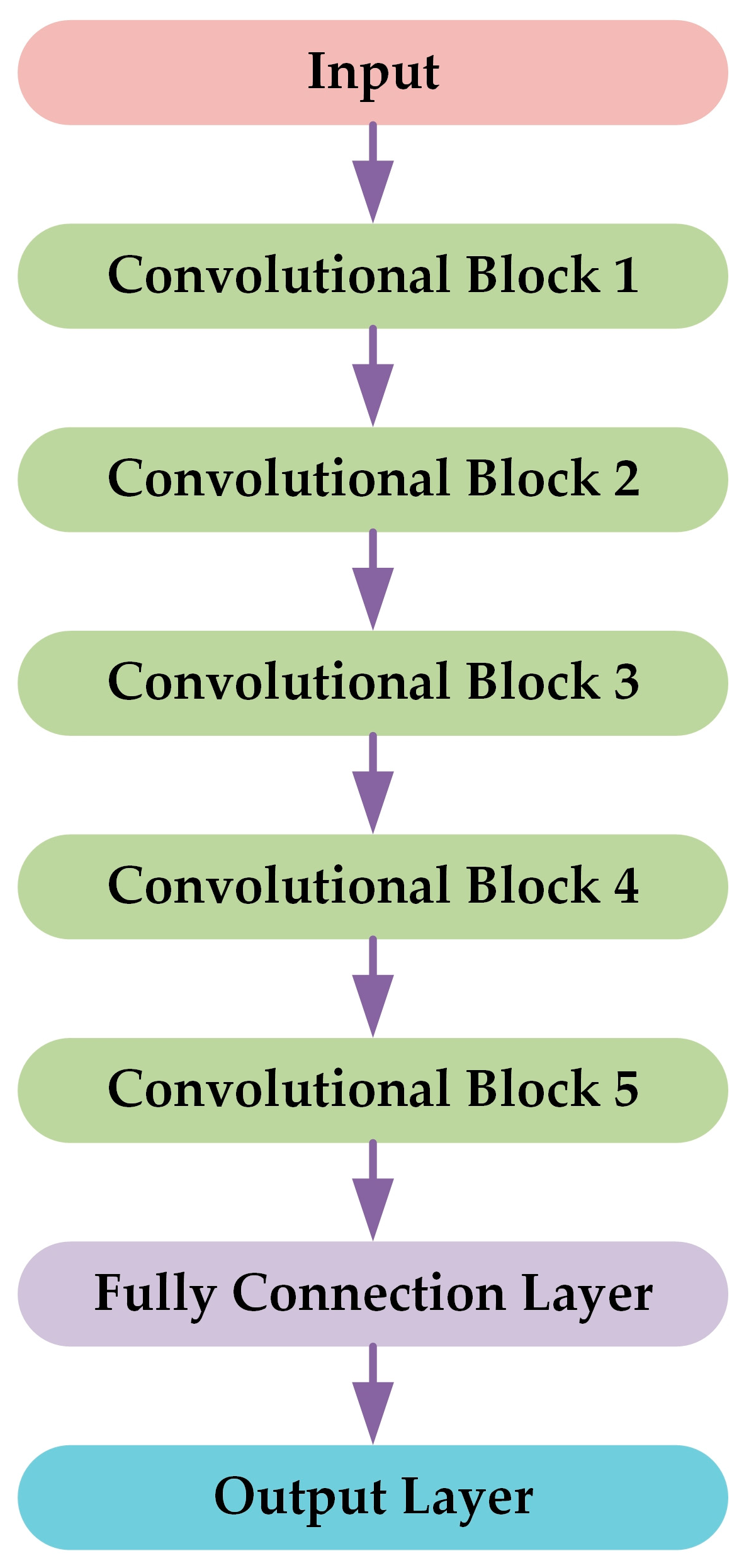
2.3. Original Recognition Model for CSR

In many studies, convolutional neural networks (CNNs) have been used for recognizing intra-pulse modulations. Unlike the recognition with ImageNet [21,22], which usually contains more than 1000 classes, there are fewer types of intra-pulse modulations. Therefore, we take a CNN model with a normal VGG-based structure [23] as the intra-pulse modulation recognition backbone. The structure of the original recognition model used in this paper is shown in Figure 3.

The input shape of the original recognition model is $128\times 128$. There are five convolutional blocks and each block contains two convolutional layers, a max-pooling layer where the stride and pooling size are 2, and a batch-normalization layer [24]. The kernel size in all convolutional blocks is 3 and the channels for convolutional block 1 to convolutional block 5 are 16, 32, 64, 128 and 256, respectively. The fully connection layer contains 256 nodes and the number of nodes of the output layer is the same as the number of known classes. Except for the output layer, which uses “softmax,” the activation function for the rest is “ReLU” [25]. At the stage of training this recognition model, the cross-entropy function is selected as the loss function.

2.4. Encoder–Decoder Model

In anomaly detection tasks, the auto-encoder models have higher reconstruction loss for the anomaly samples than the normal samples. And inspired by SegNet [26], we chose to use an encoder–decoder-based structure to compress and decompress the TFIs and revise the recognition result predicted by the original recognition model. The structure of the encoder–decoder model used in this paper is shown in Figure 4.

The input shape of the encoder–decoder model is $128\times 128$. The encoder–decoder model mainly contains two parts.

The first part is used to compress the TFIs. There are six compressed convolutional blocks in the compress-encoder part. The compressed convolutional block is the same as the convolutional block in the original recognition model in Section 3.3. The channels for compressed convolutional block 1 to compressed convolutional block 6 are 16, 32, 64, 128, 128, and 128, respectively.

The second part of the encoder–decoder model is the decompress-encoder part, which is used for up-sampling the features from the compress-encoder part and reconstructing the TFIs. There are six decompressed convolutional blocks in the decompress-encoder part. Each block includes an up-sampling layer where the rate is 2, two convolutional layers, and a batch-normalization layer. The kernel size in all decompress convolutional blocks is 3. And the channels for decompressed convolutional block 1 to decompressed convolutional block 6 are 128, 128, 128, 64, 32, and 16, respectively. The activation function used in this part is “ReLU”.

The output layer includes a convolutional layer with “Sigmoid” as the activation function, where the channel and kernel size are 1. Therefore, the output shape of the encoder–decoder model is same as the input shape. During the training session, MSE was used as the loss function.

3. Dataset and Experimental Settings

This section provides a simulation dataset of eleven different intra-pulse modulations of radar emitter signals. Then, a description of the experiments with different levels of openness is provided in detail. In addition, the two most representative methods based on OpenMax and the maximum logit score (MLS) were used as the baseline methods for intra-pulse modulation of OSR.

All programs related to the experiments were conducted with a computer with Intel 10,900 K, 128 GB RAM, and RTX 4090 GPU hardware capabilities; “MATLAB 2021a” software; and the “Keras” and “Python” programming languages.

3.1. Intra-Pulse Modulation Radar Emitter Signal Datasets

In the actual environment, the carrier frequency of a radar emitter signal could range from 300 MHz to 300 GHz. The receiver, where its local oscillators will down mix the frequency, could output the signal sequences with a lower frequency. These low-frequency signal sequences are finally aimed for analyzing and preprocessing later. Although the pulse width could range from several microseconds to a hundred microseconds, a short pulse width is more common. Therefore, in this paper, we focus on a certain range of pulse width, from 5 μs to 20 μs. Besides, assuming the bandwidth for the receiver is 100 MHz, we set a 200 MHz sampling frequency with single-channel sampling.

As a result, in this paper, we simulated eleven types of intra-pulse modulation signals, which include single-carrier frequency (SCF) signals, linear frequency modulation (LFM) signals, sinusoidal frequency modulation (SFM) signals, quadratic frequency modulation (EQFM) signals, dual linear frequency modulation (DLFM) signals, multiple linear frequency modulation (MLFM) signals, binary frequency shift keying (BFSK) signals, quadrature frequency shift keying (QFSK) signals, binary phase shift keying (BPSK) signals, Frank phase-coded (Frank) signals, and composite modulation with LFM and BPSK (LFM-BPSK) signals. The parameters of the eleven types of intra-pulse modulations are shown in

Table 1. The parameters of eleven types of intra-pulse modulations.

Type	Frequency	Parameters	Details
SCF	10 MHz–90 MHz	None	None
LFM	10 MHz–90 MHz	Bandwidth: 10 MHz–70 MHz	1. Both up LFM and down LFM are included 2. Both max value and min value of the instantaneous frequency for LFM range from 10 MHz to 70 MHz
SFM	10 MHz–90MHz	Bandwidth: 10 MHz–70 MHz	Both max value and min value of the instantaneous frequency for SFM range from 10 MHz to 70 MHz
EQFM	10 MHz–90 MHz	Bandwidth: 10 MHz–70 MHz	1. The instantaneous frequency increases first and then decreases, or decreases first and then increases 2. Both max value and min value of the instantaneous frequency for EQFM range from 10 MHz to 70 MHz
DLFM	10 MHz–90 MHz	Bandwidth: 10 MHz–70 MHz	1. The instantaneous frequency increases first and then decreases, or decreases first and then increases 2. Both max value and min value of the instantaneous frequency for DLFM range from 10 MHz to 70 MHz
MLFM	10 MHz–90 MHz 10 MHz–90 MHz	Bandwidth: 10 MHz–70 MHz Bandwidth: 10 MHz–70 MHz Segment ratio: 20–80%	1. Up LFM and down LFM are included in each of the two parts 2. Both max value and min value of the instantaneous frequency for each part of the MLFM range from 10 MHz to 70 MHz 3. The distance of the instantaneous frequency in the end of the first part and the instantaneous frequency in the start of the last part is more than 10 MHz
BFSK	10 MHz–90 MHz 10 MHz–90 MHz	5, 7, 11, 13-bit Barker code	The distance of two sub-carrier frequency is more than 10 MHz
QFSK	10 MHz–90 MHz 10 MHz–90 MHz 10 MHz–90 MHz 10 MHz–90 MHz	16-bit Frank code	The distance of each two sub-carrier frequency is more than 10 MHz
BPSK	10 MHz–90 MHz	5, 7, 11, 13-bit Barker code	None
FRANK	10 MHz–90 MHz	Phase number: 6, 7, 8	None
LFM-BPSK	10 MHz–90 MHz	Bandwidth: 10 MHz–70 MHz 5, 7, 11, 13-bit Barker code	1. Both up LFM and down LFM are included 2. Both max value and min value of the instantaneous frequency for LFM-BPSK range from 10 MHz to 70 MHz

.

The SNR for each type of intra-pulse modulation ranges from −10.5 dB to 10.5 dB. That is, there are 21 intervals of the SNR split by 1 dB. The mid value of each corresponding interval is $[-10 \mathrm{dB},-9 \mathrm{dB},\dots ,9 \mathrm{dB},10 \mathrm{dB}]$. For example, if the SNR = 2 dB, this means that the actual SNR in this interval belongs to $[1.5 \mathrm{dB},2.5 \mathrm{dB})$.

In each interval of the SNR, the number of samples for each type of intra-pulse modulation is 1500. Where 600 samples are training samples, 400 samples are validation samples and 500 samples are testing samples. Figure 5 shows the heat maps of the TFIs of eleven types of intra-pulse modulation signals when the SNR is 10 dB.

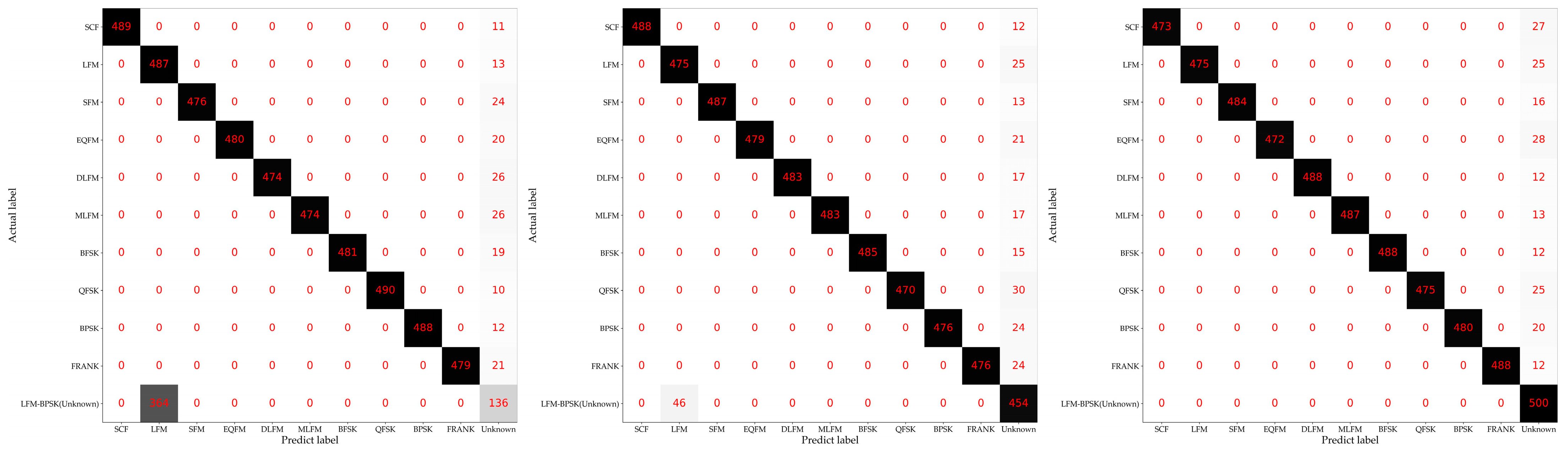
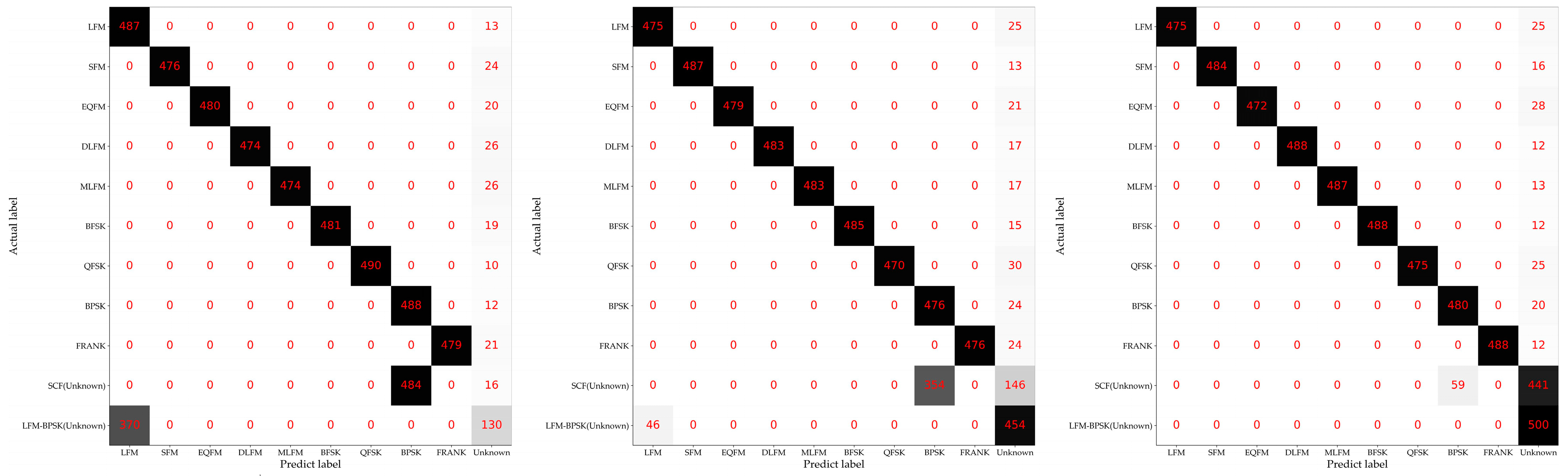
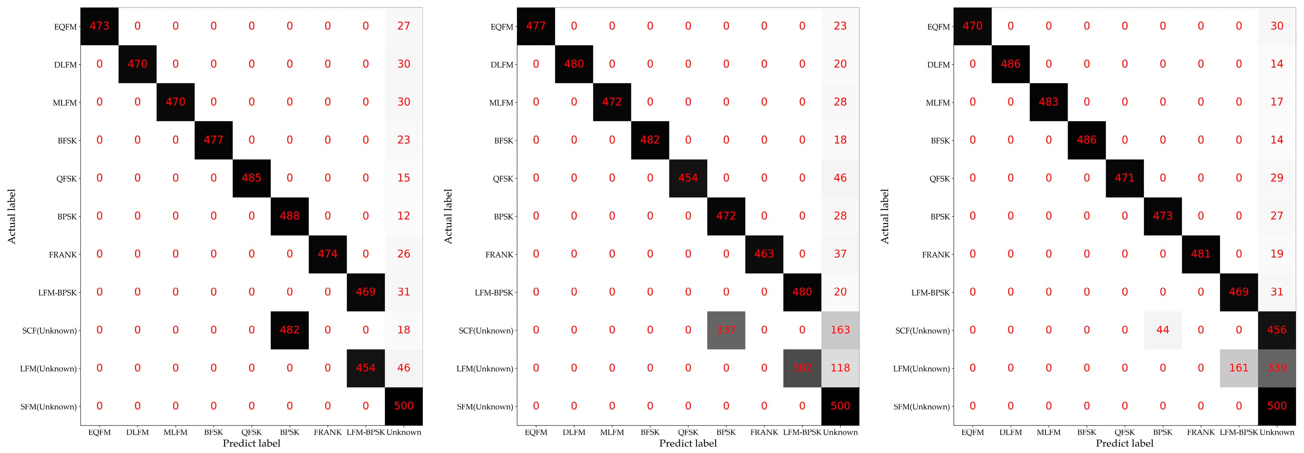
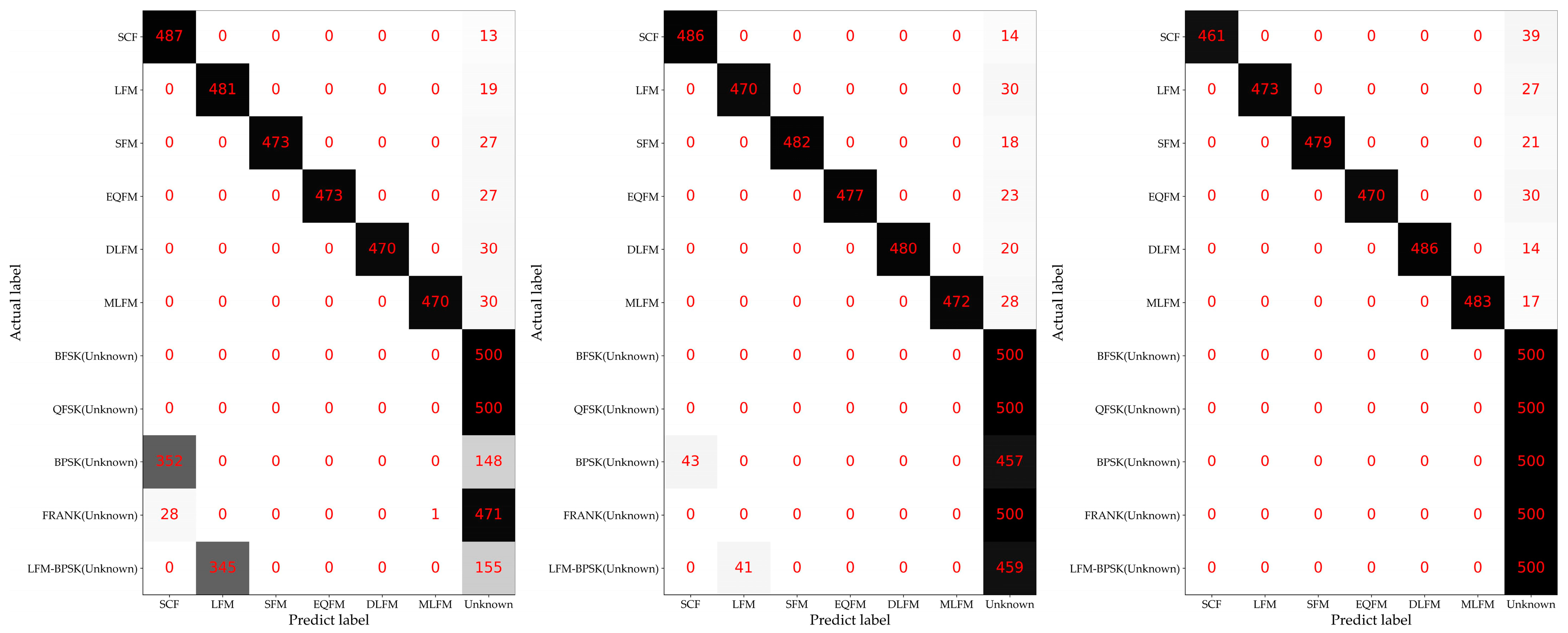
3.2. Description of the Experiments with Different Openness

In this paper, we conducted several experiments with different levels of openness to show the performance of the proposed OSR method for intra-pulse modulation. Specifically, we take five main conditions into consideration. The details of these five conditions are shown as follows:

Condition 1: Ten out of eleven types of intra-pulse modulation are known classes, and the other type is an unknown class. Therefore, there are 11 different situations in Condition 1.

Condition 2: Nine out of eleven types of intra-pulse modulation are known classes, and the other two types are unknown classes. Therefore, there are 55 different situations in Condition 2.

Condition 3: Eight out of eleven types of intra-pulse modulation are known classes, and the other three types are unknown classes. Therefore, there are 165 different situations in Condition 3.

Condition 4: Seven out of eleven types of intra-pulse modulation are known classes, and the other four types are unknown classes. Therefore, there are 330 different situations in Condition 4.

Condition 5: Six out of eleven types of intra-pulse modulation are known classes, and the other five types are unknown classes. Therefore, there are 462 different situations in Condition 5.

3.3. Baseline Methods

OpenMax has been widely used for OSR tasks. It combines deep learning with extreme theory to estimate the probability of unknown classes. In [17], the authors used STFT and OpenMax to recognize different jamming signals. Although the DNN model and the source signal are different, the OpenMax-based recognition method in [17] is still instructive. Therefore, we chose to reuse its OpenMax method accompanied by the recognition model in Section 2.3 as the baseline method. In addition, the maximum logit score (MLS) method was proven competitive with or to outperform other OSR methods in [27]. Therefore, in this paper, it was also chosen as a baseline method.

4. Experiments

4.1. Training Details and Computational Cost

The original recognition model for intra-pulse modulation CSR was trained with 20 epochs and the batch size was 64. The weights for the testing sections were chosen to have the highest overall recognition accuracy on the corresponding validation dataset.

For the encoder–decoder model, the training epoch was 300 and the batch size was 40. The optimization algorithm was all set as adaptive moment estimation (ADAM) [28] with a 0.001 learning rate. The weights, which have the lowest overall reconstruction loss on the according validation dataset, were chosen as in the testing section.

The average data preprocessing time per sample based on the method in Section 2.1 and the dataset in Section 3.1 was around 14.4 ms. The floating point operations (FLOPs), parameters, and time usage for the training and testing sessions based on the CSR model and encoder–decoder model are shown in

Table 2. The FLOPs, parameters, and time usage for the training and testing sessions based on the CSR model.

FLOPs	4.5 M
Parameters	2.2 M
Training Time/Iteration (Batch Size: 64)	13.7 ms
Forward Time (Single Sample)	2.3 ms

and

Table 3. The FLOPs, parameters, and time usage for training and testing sessions based on the encoder–decoder model.

FLOPs	3.8 M
Parameters	1.9 M
Training Time/Iteration (Batch Size: 40)	23 ms
Forward Time (Single Sample)	4.9 ms

, respectively.

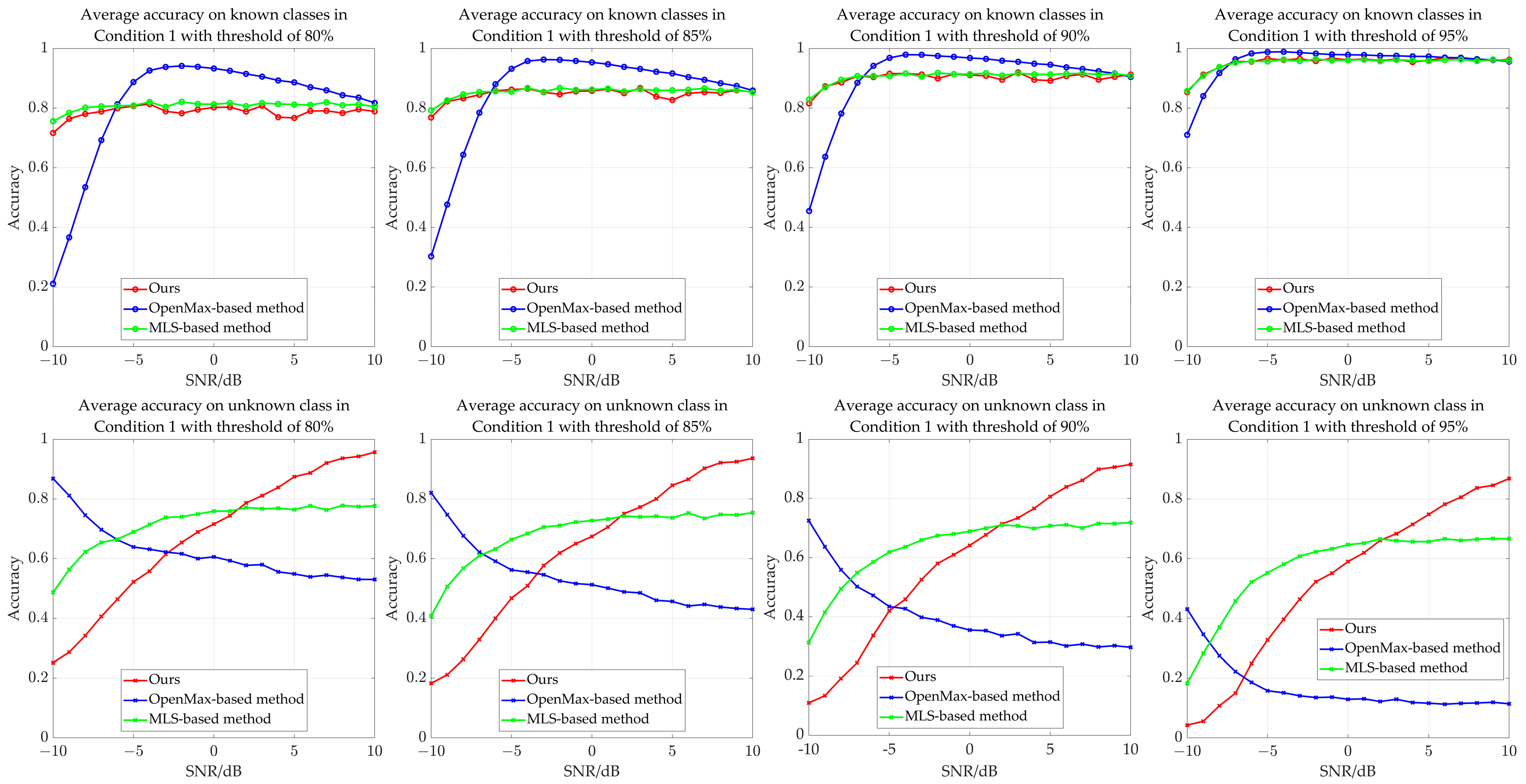
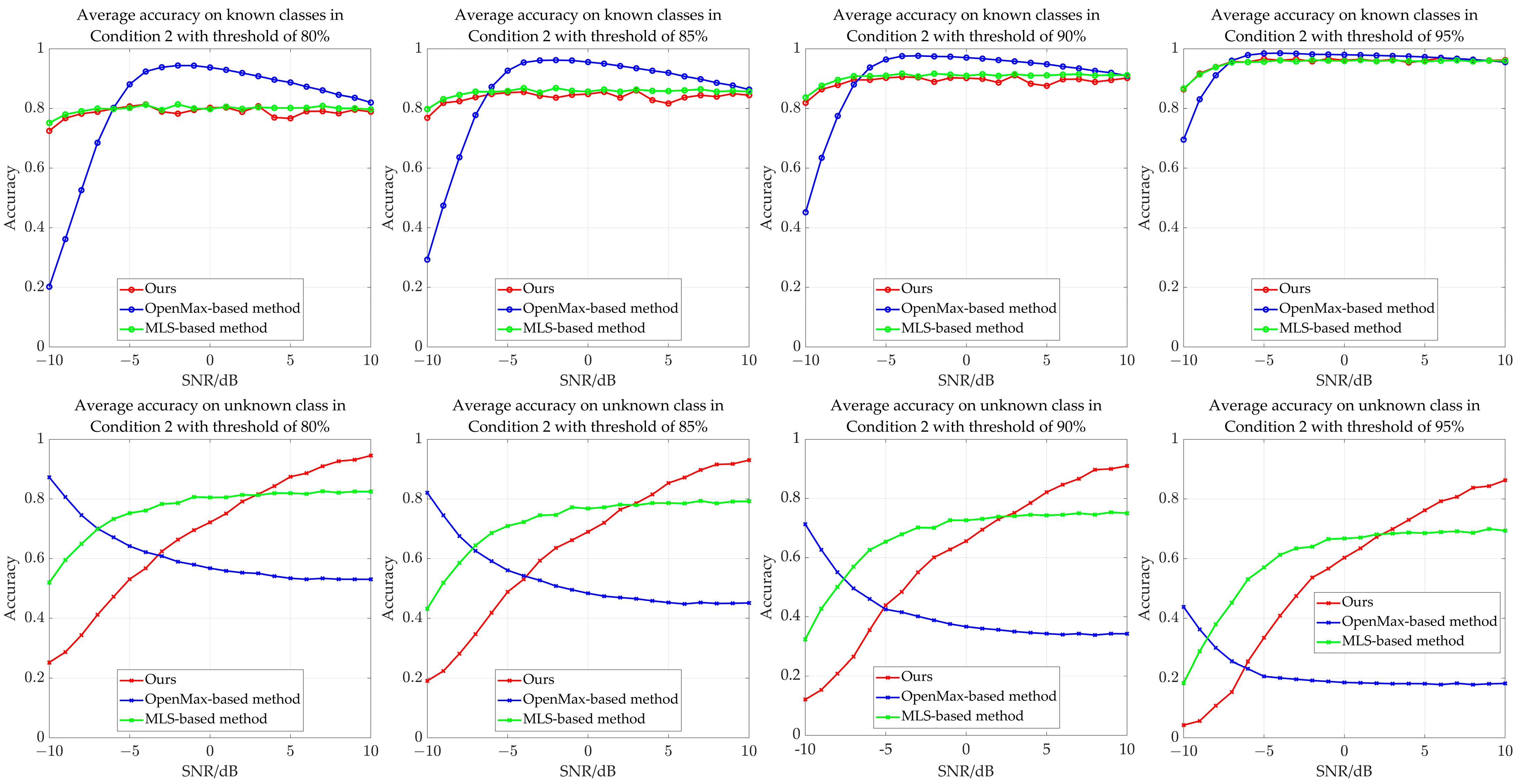
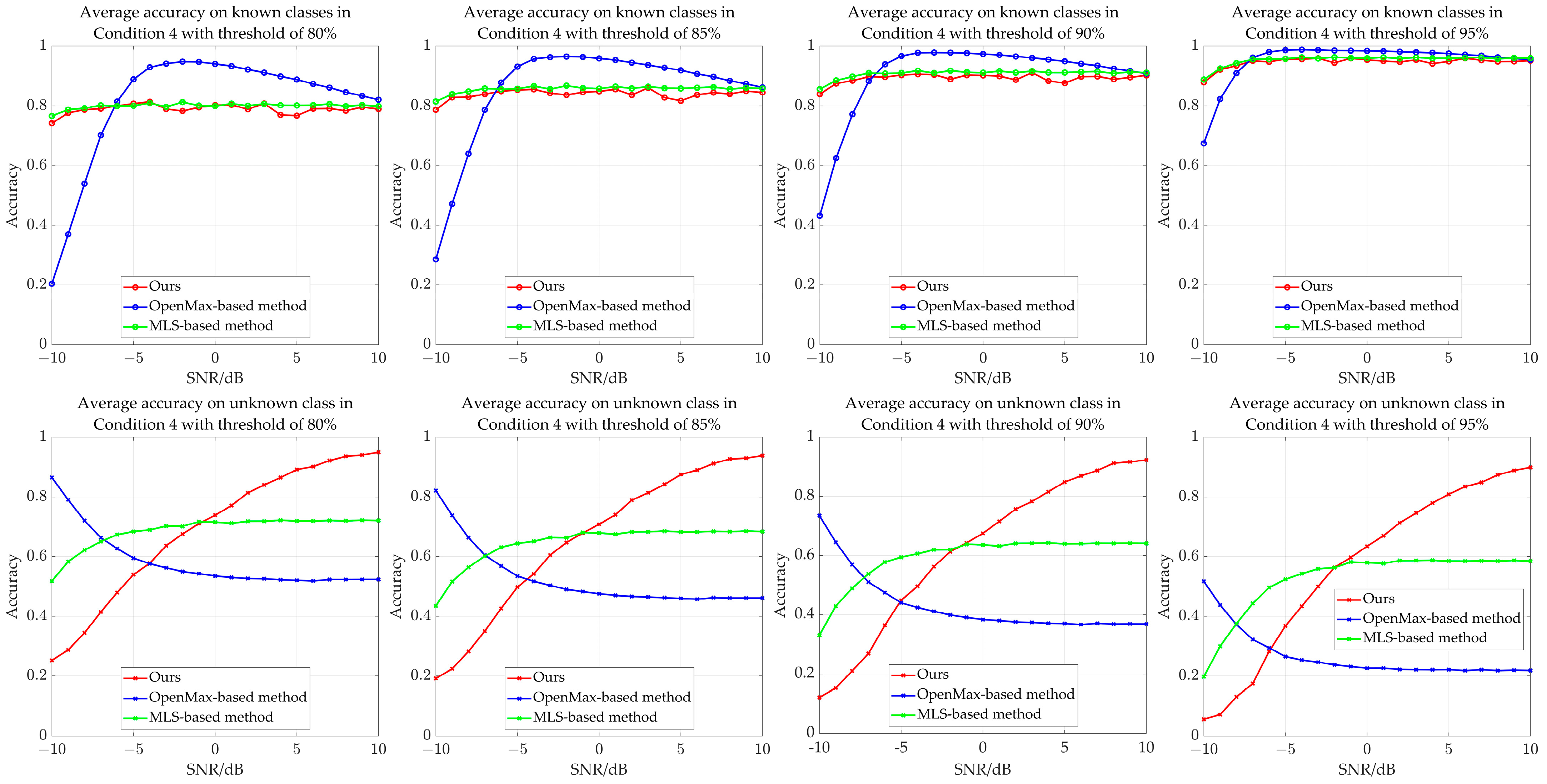
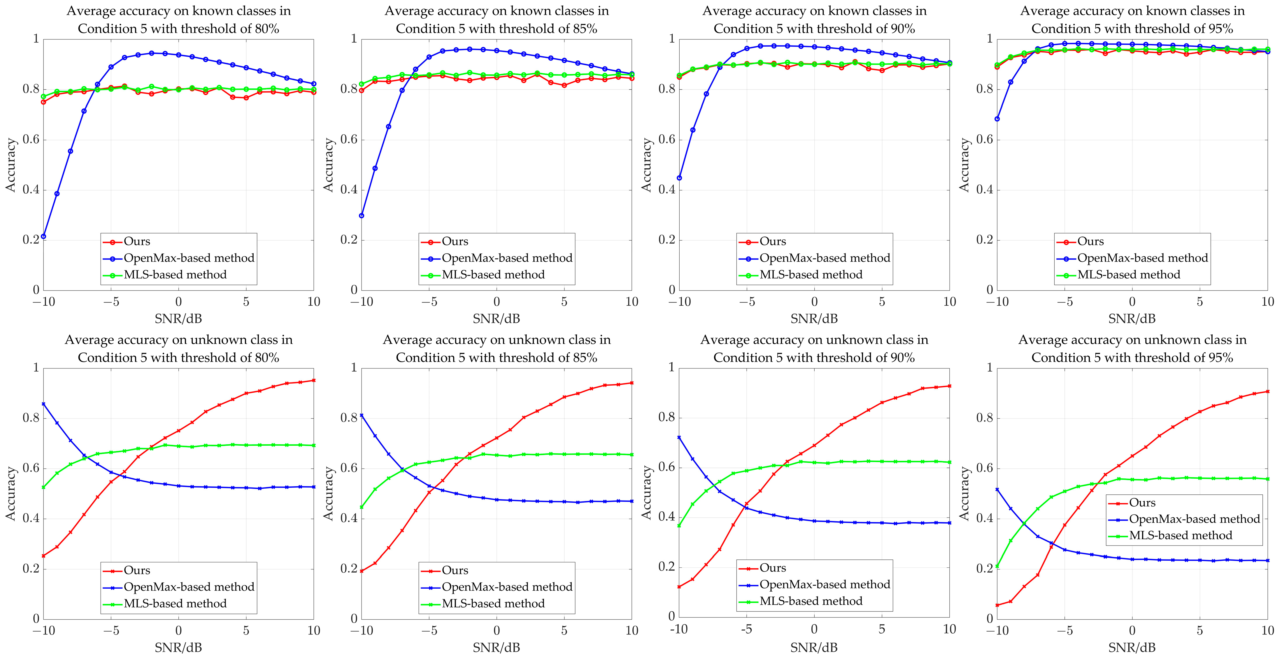
4.2. Experimental Results of the Proposed Method and Baseline Methods

Our proposed method and the baseline method were trained based on the dataset in Section 3.1 with different conditions as in Section 3.2. First of all, we provided well-trained the average recognition accuracy of the original recognition model on the corresponding known testing dataset in a closed set situation. The results are shown in

Table 4. The average recognition accuracy on the corresponding known testing dataset with different SNRs and conditions based on the original recognition models in the situation of a closed set. The number of known classes is 10, 9, 8, 7, and 6 for Condition 1 to Condition 5, respectively. The point of the SNR refers to the mean accuracy for the 1 dB interval of the SNR. The results for each condition are based on the average results of all situations in the corresponding condition. For Condition 1 to Condition 5, the number of situations is 11, 55, 165, 330, and 462, respectively.

SNR/dB	Condition 1	Condition 2	Condition 3	Condition 4	Condition 5
−10	0.8745	0.8853	0.8971	0.9081	0.9196
−9	0.9356	0.9409	0.9469	0.9529	0.9594
−8	0.9672	0.9698	0.9730	0.9761	0.9794
−7	0.9881	0.9889	0.9899	0.9911	0.9925
−6	0.9956	0.9955	0.9959	0.9964	0.9969
−5	0.9980	0.9981	0.9984	0.9984	0.9988
−4	0.9993	0.9995	0.9996	0.9995	0.9997
−3	0.9999	0.9998	0.9998	0.9999	0.9999
−2	0.9999	0.9999	0.9999	1.0000	1.0000
−1	1.0000	0.9999	0.9999	1.0000	1.0000
0	1.0000	1.0000	1.0000	1.0000	1.0000
1	1.0000	1.0000	1.0000	1.0000	1.0000
2	0.9998	0.9998	0.9999	0.9999	0.9999
3	1.0000	1.0000	1.0000	1.0000	1.0000
4	0.9999	1.0000	1.0000	1.0000	1.0000
5	1.0000	1.0000	1.0000	1.0000	1.0000
6	1.0000	1.0000	1.0000	1.0000	1.0000
7	1.0000	1.0000	1.0000	1.0000	1.0000
8	1.0000	0.9999	1.0000	1.0000	1.0000
9	1.0000	1.0000	1.0000	1.0000	1.0000
10	1.0000	1.0000	1.0000	1.0000	1.0000
Average Accuracy	0.9885	0.9894	0.9905	0.9915	0.9927

, which indicates that the original recognition model has good performance on intra-pulse modulation CSR.

Next, we conducted the experiments for the intra-pulse modulation OSR. In real actual radar systems, the average recognition accuracy on the known classes should be kept higher than or at least close to a certain value. Based on this reason, the average accuracy threshold on known classes was set to be 80%, 85%, 90%, and 95%, respectively.

Therefore, for each situation of the different conditions in Section 3.2, we set different thresholds for the reconstruction loss for our method and the score thresholds for the OpenMax-and MLS-based methods, so that the average accuracy of these methods on the corresponding validation dataset could adapt to the requirements (equal to or close to the average accuracy thresholds as much as possible).

The setting of the threshold for the OpenMax-based method and MLS-based method was based on the revised softmax score and the maximum logit score, respectively. Both methods follow the principle that if the score of the given testing sample is lower than the threshold, then the sample will be seen as unknown.

The setting of the threshold for our method is based on the principle in Section 2, where we control the ratio to ensure that the mean recognition accuracy in corresponding validation datasets is close to 80%, 85%, 90%, and 95%, respectively. Figure 6 shows the thresholds of reconstruction loss in the corresponding validation dataset with different SNRs based on these 11 encoder–decoder models when selecting 85%, 90%, and 95% samples as the known, respectively.

Then, we evaluated the above models by testing the dataset. Note that the threshold settings are all based on the corresponding validation dataset.

Figure 6 shows that a higher ratio for selecting samples as the known leads to a higher threshold for reconstruction loss. In addition, it can be seen that when the value of the SNR rises, the reconstruction loss of the corresponding validation samples based on the encoder–decoder model generally decreases.

Table 5. Under the average accuracy threshold of 80%, the average recognition accuracy of our proposed method, the OpenMax-based method and MLS-based method on the corresponding test dataset with 5 different conditions. The results for each condition are based on the average results of all situations in the corresponding condition. For Condition 1 to Condition 5, the number of situations is 11, 55, 165, 330, and 462, respectively.

Method (Average Accuracy Threshold of 80%)	Condition 1		Condition 2		Condition 3		Condition 4		Condition 5
	Known	Unknown	Known	Unknown	Known	Unknown	Known	Unknown	Known	Unknown
Ours	0.7869	0.6762	0.7876	0.6784	0.7884	0.6854	0.7891	0.6896	0.7900	0.6977
OpenMax	0.8063	0.6207	0.8058	0.6095	0.8079	0.5960	0.8100	0.5838	0.8124	0.5811
MLS	0.8077	0.7183	0.7983	0.7657	0.7992	0.7208	0.7996	0.6879	0.8003	0.6684

,

Table 6. Under the average accuracy threshold of 85%, the average recognition accuracy of our proposed method, the OpenMax-based method and MLS-based method on the corresponding test dataset with 5 different conditions. The results for each condition are based on the average results of all situations in the corresponding condition. For Condition 1 to Condition 5, the number of situations is 11, 55, 165, 330, and 462, respectively.

Method (Average Accuracy Threshold of 85%)	Condition 1		Condition 2		Condition 3		Condition 4		Condition 5
	Known	Unknown	Known	Unknown	Known	Unknown	Known	Unknown	Known	Unknown
Ours	0.8468	0.6337	0.8377	0.6444	0.8386	0.6524	0.8394	0.6575	0.8403	0.6665
OpenMax	0.8517	0.5357	0.8515	0.5308	0.8519	0.5279	0.8527	0.5248	0.8532	0.5265
MLS	0.8547	0.6842	0.8548	0.7231	0.8557	0.6797	0.8562	0.6455	0.8569	0.6267

,

Table 7. Under the average accuracy threshold of 90%, the average recognition accuracy of our proposed method, the OpenMax-based method and MLS-based method on the corresponding test dataset with 5 different conditions. The results for each condition are based on the average results of all situations in the corresponding condition. For Condition 1 to Condition 5, the number of situations is 11, 55, 165, 330, and 462, respectively.

Method (Average Accuracy Threshold of 90%)	Condition 1		Condition 2		Condition 3		Condition 4		Condition 5
	Known	Unknown	Known	Unknown	Known	Unknown	Known	Unknown	Known	Unknown
Ours	0.9000	0.5891	0.8905	0.6031	0.8915	0.6121	0.8924	0.6182	0.8934	0.6283
OpenMax	0.9014	0.4014	0.9017	0.4132	0.9018	0.4258	0.9014	0.4333	0.9012	0.4353
MLS	0.9059	0.6380	0.9060	0.6704	0.9071	0.6304	0.9077	0.5944	0.8987	0.5880

and

Table 8. Under the average accuracy threshold of 95%, the average recognition accuracy of our proposed method, the OpenMax-based method and MLS-based method on the corresponding test dataset with 5 different conditions. The results for each condition are based on the average results of all situations in the corresponding condition. For Condition 1 to Condition 5, the number of situations is 11, 55, 165, 330, and 462, respectively.

Method (Average Accuracy Threshold of 95%)	Condition 1		Condition 2		Condition 3		Condition 4		Condition 5
	Known	Unknown	Known	Unknown	Known	Unknown	Known	Unknown	Known	Unknown
Ours	0.9530	0.5248	0.9539	0.5324	0.9449	0.5576	0.9459	0.5652	0.9470	0.5767
OpenMax	0.9533	0.1667	0.9511	0.2177	0.9522	0.2407	0.9513	0.2669	0.9494	0.2793
MLS	0.9515	0.5750	0.9519	0.5951	0.9530	0.5600	0.9539	0.5242	0.9548	0.5086

give the testing results of the average recognition accuracy of the methods for known classes and unknown classes, where the average accuracy threshold for the validation dataset is 80%, 85%, 90%, and 95%, respectively. Note that if the recognition accuracy for one of situations in one of conditions cannot reach the average accuracy threshold (like 95%), for OpenMax, the revised softmax-based threshold will be 0 and for our method, the threshold of the SNR will be positive infinity.

As the results show, both of the methods have good performance in recognizing the known intra-pulse modulations. But there is a significant difference for these three methods in the average recognition accuracies in the unknown class. When the average accuracy threshold is 95%, the average recognition accuracy in the unknown class of the OpenMax-based method is at most 0.28, while our proposed OSR method and the MLS-based method perform better, where the average recognition accuracy in the unknown class is over 0.50. As the value of the average accuracy threshold decreases, the average recognition accuracy in the unknown class for the three methods increases. Besides, although the MLS-based method performs better in Condition 1 to Condition 3, when the openness rises, our method is better at recognizing the unknown samples.

The average recognition accuracy with five conditions and different SNRs is shown in Figure 7, Figure 8, Figure 9, Figure 10 and Figure 11.

From the figures, it can be seen that our OSR method and the MLS-based method are more stable than the OpenMax-based method. In contrast, the known classes accuracy of the OpenMax-based method first rises with the increment of SNR, then it drops a lot when the SNR keeps increasing. Although the accuracy for known classes based on the OpenMax-based method is higher when SNR is higher, in the situation of a lower SNR, the OpenMax-based method performs extremely poorly compared with our OSR method and the MLS-based method. In addition, the trend of the accuracy in the unknown class based on the OpenMax-based method is decreasing as the SNR increases, while the trend based on our OSR method and the MLS-based method is generally increasing. In addition, although the MLS-based method is better at lower SNR, when the SNR goes up, the average recognition accuracy in the unknown class is less competitive than our method, where the average recognition accuracy based our method in the unknown class is equal or more than 80% at 5 dB.

As a result, based on extensive experimental results with five different openness conditions, it is indicated that our proposed method, which better meets the actual requirement where the recognition of known classes is taken as the first consideration for actual radar systems, is effective for recognizing intra-pulse modulations of radar emitter signals in an open set. Figure 12, Figure 13, Figure 14, Figure 15 and Figure 16 provide some confusion matrices based on our method for one of the situations in the testing dataset when the SNR is 0 dB, 5 dB, and 10 dB in Condition 1 to Condition 5, respectively.

5. Discussion

We further analyzed the influence of the structure of the reconstruction model on recognition accuracy. The ablation experiments are based on the same dataset and conditions as in Section 3.1 and Section 3.2, and the training setting is the same as in Section 4.1. In addition, we provide some scenarios where our method could potentially be applied.

5.1. Ablation Study on the Structure of the Reconstruction Model on Recognition Accuracy

In this section, the original recognition models are same to those in Section 4.2. We changed the number of compressed convolutional blocks and decompressed convolutional blocks. Specifically, three ablation models are included. These three models are based the same encoder–decoder structure in Section 2.4. The differences are the block numbers. The details are as follows:

Ablation Model 1 (AM1): 4th to 6th compressed convolutional blocks and decompressed convolutional blocks are deleted.

Ablation Model 2 (AM2): 5th to 6th compressed convolutional blocks and decompressed convolutional blocks are deleted.

Ablation Model 3 (AM3): 6th compressed convolutional block and decompressed convolutional block are deleted.

In addition, the parameters of the reserved convolutional blocks are the same as the blocks in Section 2.4.

Except for these three models, we also applied the widely used reconstruction models named U-Net [29] and UNet3+ [30] as two extra ablation models.

Based on these reconstruction models, we conducted the intra-pulse modulation OSR experiments. The average recognition results are shown in

Table 9. Under the average accuracy threshold of 80%, the average recognition accuracy in the corresponding test dataset with 5 different conditions based on the ablation models and our proposed model. The results for each condition are based on the average results of all situations in the corresponding condition. For Condition 1 to Condition 5, the number of situations is 11, 55, 165, 330, and 462, respectively.

Method (Average Accuracy Threshold of 80%)	Condition 1		Condition 2		Condition 3		Condition 4		Condition 5
	Known	Unknown	Known	Unknown	Known	Unknown	Known	Unknown	Known	Unknown
Ours	0.7869	0.6762	0.7876	0.6784	0.7884	0.6854	0.7891	0.6896	0.7900	0.6977
AM1	0.8099	0.3696	0.8006	0.3817	0.8015	0.3818	0.8023	0.3815	0.8033	0.3790
AM2	0.8006	0.4427	0.8014	0.4504	0.8022	0.4515	0.8031	0.4520	0.8040	0.4516
AM3	0.7996	0.5993	0.8003	0.6027	0.8011	0.6091	0.8019	0.6108	0.8028	0.6134
U-Net	0.8024	0.3333	0.8031	0.3273	0.8039	0.3320	0.8047	0.3345	0.8057	0.3371
UNet3+	0.7998	0.3605	0.8005	0.3645	0.8014	0.3696	0.8022	0.3717	0.8032	0.3742

,

Table 10. Under the average accuracy threshold of 85%, the average recognition accuracy in the corresponding test dataset with 5 different conditions based on the ablation models and our proposed model. The results for each condition are based on the average results of all situations in the corresponding condition. For Condition 1 to Condition 5, the number of situations is 11, 55, 165, 330, and 462, respectively.

Method (Average Accuracy Threshold of 85%)	Condition 1		Condition 2		Condition 3		Condition 4		Condition 5
	Known	Unknown	Known	Unknown	Known	Unknown	Known	Unknown	Known	Unknown
Ours	0.8468	0.6337	0.8377	0.6444	0.8386	0.6524	0.8394	0.6575	0.8403	0.6665
AM1	0.8490	0.3421	0.8498	0.3468	0.8508	0.3473	0.8517	0.3472	0.8526	0.3446
AM2	0.8496	0.4065	0.8504	0.4141	0.8513	0.4158	0.8522	0.4168	0.8532	0.4168
AM3	0.8489	0.5620	0.8496	0.5664	0.8505	0.5736	0.8514	0.5760	0.8523	0.5793
U-Net	0.8500	0.2768	0.8508	0.2720	0.8517	0.2762	0.8526	0.2791	0.8536	0.2816
UNet3+	0.8494	0.3042	0.8501	0.3082	0.8511	0.3135	0.8519	0.3162	0.8529	0.3189

,

Table 11. Under the average accuracy threshold of 90%, the average recognition accuracy in the corresponding test dataset with 5 different conditions based on the ablation models and our proposed model. The results for each condition are based on the average results of all situations in the corresponding condition. For Condition 1 to Condition 5, the number of situations is 11, 55, 165, 330, and 462, respectively.

Method (Average Accuracy Threshold of 90%)	Condition 1		Condition 2		Condition 3		Condition 4		Condition 5
	Known	Unknown	Known	Unknown	Known	Unknown	Known	Unknown	Known	Unknown
Ours	0.9000	0.5891	0.8905	0.6031	0.8915	0.6121	0.8924	0.6182	0.8934	0.6283
AM1	0.9076	0.2937	0.8992	0.3066	0.9001	0.3074	0.9011	0.3077	0.9021	0.3053
AM2	0.9077	0.3616	0.8991	0.3765	0.9001	0.3788	0.9010	0.3801	0.9021	0.3803
AM3	0.8989	0.5161	0.8998	0.5216	0.9007	0.5299	0.9017	0.5332	0.9027	0.5374
U-Net	0.8989	0.2133	0.8997	0.2086	0.9007	0.2124	0.9016	0.2154	0.9026	0.2176
UNet3+	0.8987	0.2437	0.8995	0.2479	0.9005	0.2535	0.9014	0.2567	0.9025	0.2601

and

Table 12. Under the average accuracy threshold of 95%, the average recognition accuracy in the corresponding test dataset with 5 different conditions based on the ablation models and our proposed model. The results for each condition are based on the average results of all situations in the corresponding condition. For Condition 1 to Condition 5, the number of situations is 11, 55, 165, 330, and 462, respectively.

Method (Average Accuracy Threshold of 95%)	Condition 1		Condition 2		Condition 3		Condition 4		Condition 5
	Known	Unknown	Known	Unknown	Known	Unknown	Known	Unknown	Known	Unknown
Ours	0.9530	0.5248	0.9539	0.5324	0.9449	0.5576	0.9459	0.5652	0.9470	0.5767
AM1	0.9560	0.2457	0.9473	0.2615	0.9484	0.2628	0.9494	0.2633	0.9505	0.2612
AM2	0.9563	0.3089	0.9473	0.3276	0.9484	0.3304	0.9494	0.3322	0.9505	0.3326
AM3	0.9576	0.4428	0.9492	0.4650	0.9502	0.4744	0.9512	0.4787	0.9523	0.4837
U-Net	0.9563	0.1223	0.9472	0.1371	0.9483	0.1400	0.9492	0.1427	0.9503	0.1442
UNet3+	0.9565	0.1547	0.9574	0.1582	0.9487	0.1809	0.9497	0.1848	0.9508	0.1890

. In addition, we summarized the average reconstruction loss on the corresponding validation dataset in

Table 13. The average reconstruction loss in the corresponding validation dataset based on the ablation models and our proposed model. As there are 11 types of intra-pulse modulations, the results for each reconstruction model are based on the average results of 11 sub-reconstruction encoder–decoder models. As the original loss is based on MSE, which is too small, we report it by magnifying itself 16,384 times (equal to 128 × 128).

Reconstruction Model	Ours	AM1	AM2	AM3	U-Net	UNet3+
Average Reconstruction Loss (The original value based on MSE is magnified 16,384 times (equals to 128 × 128))	36.7777	4.5015	10.3470	24.0721	0.0294	0.0333

.

From Table 9, Table 10, Table 11, Table 12 and Table 13, it could be found that the deeper structure of the proposed encoder–decoder model provides better performance in recognizing the unknown intra-pulse modulation. In addition, the experimental results of AM1 to AM3 and ours show that the structure of the encoder–decoder will obtain more reconstruction loss when the depth increases. In addition, the average reconstruction loss of the U-Net model and UNet3+ model is quite low, compared among the Ablation Model 1 to Ablation Model 3 and the model in Section 2.4, which means these two models reconstruct the TFIs in high quality.

However, although these two models with complex structures have lower reconstruction loss in the validation dataset, they do not provide good performance in recognizing the unknown intra-pulse modulation. The reason for this is that the merging connection from the encoder part to the decoder part keeps many shallower features, where the decoder part receives many features without deep compression. If the model receives an unknown sample, due to the merging connection, the output will still have low reconstruction loss.

The encoder–decoder structure in Section 2.4, which does not have an extra connection branch, extremely compresses the feature used for the decoder part. Therefore, the output reconstructed TFIs have higher reconstruction loss. If this model receives an unknown sample, then a very slight change from the output of its encoder part will cause a higher difference in the output result, reflected in the higher reconstruction loss compared with the unknown samples.

In terms of the intra-pulse modulation OSR, our proposed structure of an encoder–decoder model without an extra merging connection is more suitable and effective for recognizing the unknown class.

5.2. Application Scenarios

DNN-based models have been widely used for radar emitter signal intra-pulse modulation recognition. In real applications, except for the known classes, radar systems are often facing unknown intra-pulse modulations. It is essential for the systems not only to classify the known classes in the library correctly, but also to identify the unknown samples. Currently, there are few pieces of literature focusing on OSR in radar emitter signal intra-pulse modulation. Through the result of Table 5, Table 6, Table 7, Table 8, Table 9, Table 10, Table 11 and Table 12 in Section 4.2 and Section 5.1, we could reach a conclusion that a deeper encoder–decoder structure without an extra merging connection could increase the performance in recognizing unknown intra-pulse modulation.

At the same time, our method could be applied to other radar signal recognition tasks. For example, in radar jamming recognition tasks [17,31], the library cannot include all of the jamming types from the target jamming emitter. Therefore, it is important to accurately classify the known jamming types and recognize the unknown jamming. Besides, automatic target recognition based on synthetic aperture radar images [32] and high-resolution range profile recognition [33] is also facing the problem that unknown targets often emerge and cannot be neglected. Correctly recognizing the unknown targets will provide better intelligence for the systems. Although the source data for different radar signal recognition tasks are different, the framework of our method, like threshold setting and an encoder–decoder model for revising the recognition result, still could provide guidance for designing corresponding recognition methods.

6. Conclusions

In this paper, we focused on an open set situation instead of a closed set situation and proposed a method for recognizing radar emitter signal intra-pulse modulations. Through the extensive experiments, including five different openness conditions, we found that our proposed method, which combines data preprocessing based on STFT, SNR estimation, a recognition model for CSR, and an encoder–decoder model, is effective in recognizing an unknown intra-pulse modulation with good performance in classifying known intra-pulse modulations. Additionally, according to an ablation study of the effect of the structure of the reconstruction model on recognition accuracy, we could conclude that a deeper encoder–decoder structure without extra merging connections leads to better performance in recognizing unknown samples. Our proposed method in this paper could provide guidance for radar emitter signal intra-pulse modulation OSR tasks.

As the current method only recognizes unknown samples from different types as one unknown class, in future work, we will focus on the task of classifying these unknown samples into specific classes.

References

1. Zhao, G. Principle of Radar Countermeasure, 2nd ed.; Xidian University Press: Xi’an, China, 2012. [Google Scholar]
2. Richards, M.A. Fundamentals of Radar Signal Processing, 2nd ed.; McGraw-Hill Education: New York, NY, USA, 2005. [Google Scholar]
3. Barton, D.K. Radar System Analysis and Modeling; Artech: London, UK, 2004. [Google Scholar]
4. Wiley, R.G.; Ebrary, I. ELINT: The Interception and Analysis of Radar Signals; Artech: London, UK, 2006. [Google Scholar]
5. Qu, Z.; Mao, X.; Deng, Z. Radar Signal Intra-Pulse Modulation Recognition Based on Convolutional Neural Network. IEEE Access 2018, 6, 43874–43884. [Google Scholar] [CrossRef]
6. Yu, Z.; Tang, J.; Wang, Z. GCPS: A CNN Performance Evaluation Criterion for Radar Signal Intrapulse Modulation Recognition. IEEE Commun. Lett. 2021, 25, 2290–2294. [Google Scholar] [CrossRef]
7. Yuan, S.; Wu, B.; Li, P. Intra-Pulse Modulation Classification of Radar Emitter Signals Based on a 1-D Selective Kernel Convolutional Neural Network. Remote Sens. 2021, 13, 2799. [Google Scholar] [CrossRef]
8. Wu, B.; Yuan, S.; Li, P.; Jing, Z.; Huang, S.; Zhao, Y. Radar Emitter Signal Recognition Based on One-Dimensional Convolutional Neural Network with Attention Mechanism. Sensors 2020, 20, 6350. [Google Scholar] [CrossRef]
9. Si, W.; Wan, C.; Deng, Z. Intra-Pulse Modulation Recognition of Dual-Component Radar Signals Based on Deep Convolutional Neural Network. IEEE Commun. Lett. 2021, 25, 3305–3309. [Google Scholar] [CrossRef]
10. Tan, M.; Le, Q. Efficientnet: Rethinking model scaling for convolutional neural networks. In Proceedings of the International Conference on Machine Learning, Long Beach, CA, USA, 9–15 June 2019; pp. 6105–6114. [Google Scholar]
11. Wan, C.; Si, W.; Deng, Z. Research on modulation recognition method of multi-component radar signals based on deep convolution neural network. IET Radar Sonar Navig. 2023, 17, 1313–1326. [Google Scholar] [CrossRef]
12. Cai, J.; He, M.; Cao, X.; Gan, F. Semi-Supervised Radar Intra-Pulse Signal Modulation Classification With Virtual Adversarial Training. IEEE Internet Things J. 2023. [Google Scholar] [CrossRef]
13. Yuan, S.; Li, P.; Wu, B.; Li, X.; Wang, J. Semi-Supervised Classification for Intra-Pulse Modulation of Radar Emitter Signals Using Convolutional Neural Network. Remote Sens. 2022, 14, 2059. [Google Scholar] [CrossRef]
14. Hendrycks, D.; Gimpel, K. A baseline for detecting misclassified and out-of-distribution examples in neural networks. arXiv 2016, arXiv:1610.02136. [Google Scholar]
15. Bendale, A.; Boult, T.E. Towards Open Set Deep Networks. In Proceedings of the 2016 IEEE Conference on Computer Vision and Pattern Recognition (CVPR), Las Vegas, NV, USA, 27–30 June 2016; pp. 1563–1572. [Google Scholar] [CrossRef]
16. Sun, C.; Du, Y.; Qiao, X.; Wu, H.; Zhang, T. Research on the Enhancement Method of Specific Emitter Open Set Recognition. Electronics 2023, 12, 4399. [Google Scholar] [CrossRef]
17. Zhou, Y.; Shang, S.; Song, X.; Zhang, S.; You, T.; Zhang, L. Intelligent Radar Jamming Recognition in Open Set Environment Based on Deep Learning Networks. Remote Sens. 2022, 14, 6220. [Google Scholar] [CrossRef]
18. Auger, F.; Flandrin, P. Improving the readability of time-frequency and time-scale representations by the reassignment method. IEEE Trans. Signal Process. 1995, 43, 1068–1089. [Google Scholar] [CrossRef]
19. Wang, X.; Huang, G.; Zhou, Z.; Tian, W.; Yao, J.; Gao, J. Radar Emitter Recognition Based on the Energy Cumulant of Short Time Fourier Transform and Reinforced Deep Belief Network. Sensors 2018, 18, 3103. [Google Scholar] [CrossRef] [PubMed]
20. Hoang, L.M.; Kim, M.; Kong, S.-H. Automatic Recognition of General LPI Radar Waveform Using SSD and Supplementary Classifier. IEEE Trans. Signal Process. 2019, 67, 3516–3530. [Google Scholar] [CrossRef]
21. Szegedy, C.; Liu, W.; Jia, Y.; Sermanet, P.; Reed, S.; Anguelov, D.; Erhan, D.; Vanhoucke, V.; Rabinovich, A. Going deeper with convolutions. In Proceedings of the 2015 IEEE Conference on Computer Vision and Pattern Recognition (CVPR), Boston, MA, USA, 7–12 June 2015; pp. 1–9. [Google Scholar] [CrossRef]
22. He, K.; Zhang, X.; Ren, S.; Sun, J. Deep Residual Learning for Image Recognition. In Proceedings of the 2016 IEEE Conference on Computer Vision and Pattern Recognition (CVPR), Las Vegas, NV, USA, 27–30 June 2016; pp. 770–778. [Google Scholar] [CrossRef]
23. Simonyan, K.; Zisserman, A. Very deep convolutional networks for large-scale image recognition. arXiv 2014, arXiv:1409.1556. [Google Scholar]
24. Ioffe, S.; Szegedy, C. Batch normalization: Accelerating deep network training by reducing internal covariate shift. arXiv 2015, arXiv:1502.03167. [Google Scholar]
25. Nair, V.; Hinton, G.E. Rectified linear units improve restricted boltzmann machines. In Proceedings of the 27th International Conference on Machine Learning (ICML-10), Haifa, Israel, 21–24 June 2010. [Google Scholar]
26. Badrinarayanan, V.; Kendall, A.; Cipolla, R. SegNet: A Deep Convolutional Encoder-Decoder Architecture for Image Segmentation. IEEE Trans. Pattern Anal. Mach. Intell. 2017, 39, 2481–2495. [Google Scholar] [CrossRef] [PubMed]
27. Vaze, S.; Han, K.; Vedaldi, A.; Zisserman, A. Open-set recognition: A good closed-set classifier is all you need. arXiv 2021, arXiv:2110.06207. [Google Scholar]
28. Kingma, D.P.; Ba, J. Adam: A Method for Stochastic Optimization. arXiv 2014, arXiv:1412.6980. [Google Scholar]
29. Ronneberger, O.; Fischer, P.; Brox, T. U-net: Convolutional networks for biomedical image segmentation. In Proceedings of the International Conference on Medical Image Computing and Computer-Assisted Intervention, Munich, Germany, 5–9 October 2015; Springer: Cham, Switzerland, 2015; pp. 234–241. [Google Scholar]
30. Huang, H.; Lin, L.; Tong, R.; Hu, H.; Zhang, Q.; Iwamoto, Y.; Han, X.; Chen, Y.-W.; Wu, J. UNet 3+: A Full-Scale Connected UNet for Medical Image Segmentation. In Proceedings of the ICASSP 2020—2020 IEEE International Conference on Acoustics, Speech and Signal Processing (ICASSP), Barcelona, Spain, 4–8 May 2020; pp. 1055–1059. [Google Scholar] [CrossRef]
31. Lv, Q.; Quan, Y.; Feng, W.; Sha, M.; Dong, S.; Xing, M. Radar Deception Jamming Recognition Based on Weighted Ensemble CNN With Transfer Learning. IEEE Trans. Geosci. Remote Sens. 2022, 60, 5107511. [Google Scholar] [CrossRef]
32. Zhou, X.; Bai, X.; Xue, R. ISAR Target Recognition Based on Capsule Net. In Proceedings of the 2021 CIE International Conference on Radar (Radar), Haikou, China, 15–19 December 2021; pp. 39–42. [Google Scholar] [CrossRef]
33. Guo, D.; Chen, B.; Chen, W.; Wang, C.; Liu, H.; Zhou, M. Variational Temporal Deep Generative Model for Radar HRRP Target Recognition. IEEE Trans. Signal Process. 2020, 68, 5795–5809. [Google Scholar] [CrossRef]
Figure 1. A flow chart of the proposed intra-pulse modulation OSR method.
Remotesensing 16 00108 g001
Figure 2. A sketch map of the proposed method in actual deployment. For a given sample, the well-trained original recognition model for CSR will label it a certain known class temporarily. Through estimating the SNR of the sample and calculating the reconstruction loss by inputting the sample to the corresponding encoder–decoder model related to the temporary predicted known class, whether the sample belongs to the predicted temporary known class or the unknown class will be confirmed.
Remotesensing 16 00108 g002
Figure 3. The structure of the original recognition model used in this paper.
Remotesensing 16 00108 g003
Figure 4. The structure of the encoder–decoder model used in this paper.
Remotesensing 16 00108 g004
Figure 5. The heat maps of the TFIs of eleven types of intra-pulse modulation signals when the SNR is 10 dB.
Remotesensing 16 00108 g005
Figure 6. The thresholds of reconstruction loss in the corresponding validation datasets with different SNRs based on these 11 encoder–decoder models when selecting 85%, 90%, and 95% samples as the known, respectively, which equals to setting the top highest 15%, 10%, and 5% reconstruction losses from the corresponding validation samples as the thresholds in each interval of the SNR in one known class. The marker point refers to the accuracy for the 1 dB interval of the SNR.
Remotesensing 16 00108 g006
Figure 7. The average recognition accuracy of our proposed method, the OpenMax-based method, and the MLS-based method on the according test dataset for different SNRs in Condition 1. The marker point refers to the accuracy for the 1 dB interval of the SNR. The results are based on the average results of 11 situations in Condition 1. “Threshold of 80%, 85%, 90%, and 95%” means the average accuracy in the corresponding validation dataset with known classes is 80%, 85%, 90%, and 95%, respectively.
Remotesensing 16 00108 g007
Figure 8. The average recognition accuracy of our proposed method, the OpenMax-based method, and the MLS-based method in the corresponding test dataset for different SNRs in Condition 2. The marker point refers to the accuracy for the 1 dB interval of the SNR. The results are based on the average results of 55 situations in Condition 2. “Threshold of 80%, 85%, 90%, and 95%” means the average accuracy in the corresponding validation dataset with known classes is 80%, 85%, 90%, and 95%, respectively.
Remotesensing 16 00108 g008
Figure 9. The average recognition accuracy of our proposed method, the OpenMax-based method, and the MLS-based method in the corresponding test dataset for different SNRs in Condition 3. The marker point refers to the accuracy for the 1 dB interval of the SNR. The results are based on the average results of 165 situations in Condition 3. “Threshold of 80%, 85%, 90%, and 95%” means the average accuracy in the corresponding validation dataset with known classes is 80%, 85%, 90%, and 95%, respectively.
Remotesensing 16 00108 g009
Figure 10. The average recognition accuracy of our proposed method, the OpenMax-based method, and the MLS-based method in the corresponding test dataset for different SNRs in Condition 4. The marker point refers to the accuracy for the 1 dB interval of the SNR. The results are based on the average results of 330 situations in Condition 4. “Threshold of 80%, 85%, 90%, and 95%” means the average accuracy in the corresponding validation dataset with known classes is 80%, 85%, 90%, and 95%, respectively.
Remotesensing 16 00108 g010
Figure 11. The average recognition accuracy of our proposed method, the OpenMax-based method, and the MLS-based method in the corresponding test dataset for different SNRs in Condition 5. The marker point refers to the accuracy for the 1 dB interval of the SNR. The results are based on the average results of 462 situations in Condition 5. “Threshold of 80%, 85%, 90%, and 95%” means the average accuracy in the corresponding validation dataset with known classes is 80%, 85%, 90%, and 95%, respectively.
Remotesensing 16 00108 g011
Figure 12. The confusion matrix based on our method for one of the situations in the testing dataset when the SNR is 0 dB, 5 dB, and 10 dB (from left to right) in Condition 1. In this situation, LFM-BPSK is selected as the unknown class. Darker background colors represent more quantities.
Remotesensing 16 00108 g012
Figure 13. The confusion matrix based on our method for one of the situations in the testing dataset when the SNR is 0 dB, 5 dB, and 10 dB (from left to right) in Condition 2. In this situation, SCF and LFM-BPSK are selected as the unknown classes. Darker background colors represent more quantities.
Remotesensing 16 00108 g013
Figure 14. The confusion matrix based on our method for one of the situations in the testing dataset when the SNR is 0 dB, 5 dB, and 10 dB (from left to right) in Condition 3. In this situation, SCF, LFM and SFM are selected as the unknown classes. Darker background colors represent more quantities.
Remotesensing 16 00108 g014
Figure 15. The confusion matrix based on our method for one of the situations in the testing dataset when the SNR is 0 dB, 5 dB, and 10 dB (from left to right) in Condition 4. In this situation, LFM, SFM, EQFM, and DLFM are selected as the unknown classes. Darker background colors represent more quantities.
Remotesensing 16 00108 g015
Figure 16. The confusion matrix based on our method for one of the situations in the testing dataset when the SNR is 0 dB, 5 dB, and 10 dB (from left to right) in Condition 5. In this situation, BFSK, QFSK, BPSK, FRANK and LFM-BPSK are selected as the unknown classes. Darker background colors represent more quantities.
Remotesensing 16 00108 g016