Genetic Programming Guided Mapping of Forest Canopy Height by Combining LiDAR Satellites with Sentinel-1/2, Terrain, and Climate Data

Abstract

Accurately mapping the forest canopy height is vital for conserving forest ecosystems. Employing the forest height measured by satellite light detection and ranging (LiDAR) systems as ground samples to establish forest canopy height extrapolation (FCHE) models presents promising opportunities for mapping large-scale wall-to-wall forest canopy height. However, despite the potential to provide more samples and alleviate the stripe effect by synergistically using the data from two existing LiDAR datasets, Global Ecosystem Dynamics Investigation (GEDI) and Ice, Cloud, and land Elevation Satellite-2 (ICESat-2), the fundamental differences in their operating principles create measurement biases, and thus, there are few studies combining them for research. Furthermore, previous studies have typically employed existing regression algorithms as FCHE models to predict forest canopy height, without customizing a model that achieves optimal performance based on the current samples. These shortcomings constrain the accuracy of predicting forest canopy height using satellite LiDAR data. To surmount these difficulties, we proposed a genetic programming (GP) guided method for mapping forest canopy height by combining the GEDI and ICESat-2 LiDAR data with Sentinel-1/2, terrain, and climate data. In this method, GP autonomously constructs the fusion model of the GEDI and ICESat-2 datasets (hereafter GIF model) and the optimal FCHE model based on the explanatory variables for the specific study area. The outcomes demonstrate that the fusion of the GEDI and ICESat-2 data shows high consistency (${\mathrm{R}}^2$ = 0.85, RMSE = $2.2$ $\mathrm{m}$, pRMSE = 11.24%). The synergistic use of the GEDI and ICESat-2 data, coupled with the optimization of the FCHE model, substantially improves the precision of forest canopy height predictions, and finally achieves ${\mathrm{R}}^2$, RMSE, and pRMSE of 0.64, $3.38$ $\mathrm{m}$, and 16.08%, respectively. In summary, our research presents a reliable approach to accurately estimate forest canopy height using remote sensing data by addressing measurement biases between the GEDI and ICESat-2 data and overcoming the limitations of traditional FCHE models.

1. Introduction

Forest canopy height refers to the distance from the top of the tree crowns to the ground level of trees in a forest. Since it is closely related to climate, hydrology, and biogeochemical cycles in forest ecosystems [1,2], accurate measurement of forest canopy height is vital for comprehending the structure and function of forest ecosystems, studying their carbon and water cycling processes, assessing forest responses to climate change, and monitoring changes in forest carbon stocks [3,4,5]. Furthermore, as an essential characteristic of forest structure, precise measurement of forest canopy height contributes to insights into forest growth and succession dynamics, providing a scientific foundation for forest conservation and management to achieve the sustainable development of forest ecosystems [6,7].

Remote sensing (RS) technology is an essential tool for measuring forest canopy height. In contrast to field-based measurements, RS technology can enhance measurement efficiency, diminish workload, and surmount the challenges that are typically encountered during field measurements [8,9]. Currently, a variety of RS technologies, including light detection and ranging (LiDAR), optical stereo photogrammetry, and radar interferometry, are widely employed for forest canopy height assessment [10,11,12]. Among these techniques, LiDAR obtains accurate three-dimensional (3D) forest structural information by emitting laser beams to penetrate the forest canopy [5,13]. LiDAR technology can be categorized as ground-based, airborne, and satellite LiDAR, contingent upon the platform utilized for sensor deployment [14]. The first two are ideal for small-scale observation, acquiring wall-to-wall high-resolution 3D data for accurate forest canopy height measurement [15,16]. However, constrained by cost, operational conditions, and spatial coverage, ground-based and airborne LiDAR are unsuitable for acquiring large-scale forest canopy height data [5,17,18]. In contrast, satellite LiDAR offers the advantage of delivering accurate 3D data on a global scale, particularly in remote or inaccessible areas. Moreover, spaceborne LiDAR remains unaffected by environmental factors such as weather and illumination, ensuring consistent data provision under all-weather conditions [13,19].

The first LiDAR satellite, Ice, Cloud, and Land Elevation Satellite (ICESat-1), was launched in 2003, and its onboard instrument, the Geoscience Laser Altimeter System (GLAS), served as a critical data source for mapping forest canopy height globally. It ceased operation in 2009 [20]. The next-generation spaceborne LiDAR sensors, ICESat-2 and Global Ecosystem Dynamics Investigation (GEDI), were launched in 2018, offering denser and higher spatial resolution ground footprints compared to ICESat-1 [12]. However, it is noteworthy that similar to ICESat-1, the data from ICESat-2 and GEDI are still discretely distributed along their observation orbits rather than being spatially continuous. Therefore, it is impossible to predict wall-to-wall forest canopy height using only spaceborne LiDAR data [7]. To surmount this obstacle, existing studies have attempted to use LiDAR-derived forest canopy height as the response variable and several image features related to forest height from spatially continuous data, such as multispectral images, as explanatory variables [5,21]. Regression algorithms with promising prediction performance, including random forest (RF), support vector machine (SVM), and decision tree (DT), have been employed as the forest canopy height extrapolation (FCHE) model to achieve spatially continuous predictions of forest canopy height [2,19].

Although prior research results have confirmed the feasibility of utilizing ICESat-2 or GEDI height data as ground truth and machine learning (ML) algorithms as the FCHE model to achieve wall-to-wall mapping of forest canopy height [4,6,16,22], two major limitations remain in this process that adversely affect the accuracy of predictions and transferability of the methods. First, the distinct disparities encompassing the operational principles, measurement precision, and data processing approaches of ICESat-2 and GEDI engender biases in their respective height measurements at identical locations. Consequently, limited research has attempted concurrently utilizing these two spaceborne LiDAR datasets [14]. However, the advantages of using these two datasets together are apparent, as this not only enhances the number of ground samples but also reduces the strong stripe effect arising from the trackwise distribution of LiDAR data in the regression results, thereby facilitating the improvement in predictive accuracy [7,14]. Second, the majority of the FCHE models used in existing studies are determined by researchers subjectively based on past research experiences [16,23]. It should be noted that the performance of the same regressor varies from different regression tasks. Therefore, it cannot be assumed that the regression model selected based on prior research experience is the optimal FCHE model for the present regression task. Symbolic regression (SR) techniques, represented by the genetic programming (GP) algorithm, have been recently applied successfully to construct models for predicting multiple ecological indicators, such as air [24] and water quality [25]. These models constructed by SR exhibit high transferability and superior performance in solving high-dimensional and nonlinear problems [26,27], indicating the strong potential of these techniques for constructing promising GEDI and ICESat-2 fusion models (hereinafter GIF models) and FCHE models.

In our research, we attempted to propose a forest canopy height estimation method that integrates ICESat-2 and GEDI satellite LiDAR data with Sentinel-1/2, topographic, and climatic data guided by GP. In this method, GP was used to construct the GIF and FCHE models that performed optimally in this study. Our objectives for this research are (1) to evaluate the effectiveness of GP in constructing the GIF and FCHE models, (2) to explore the potential of combining the ICESat-2 and GEDI data and optimizing the FCHE model in improving the accuracy of forest canopy height prediction, and (3) to assess the transferability of this method.

2. Study Sites and Data

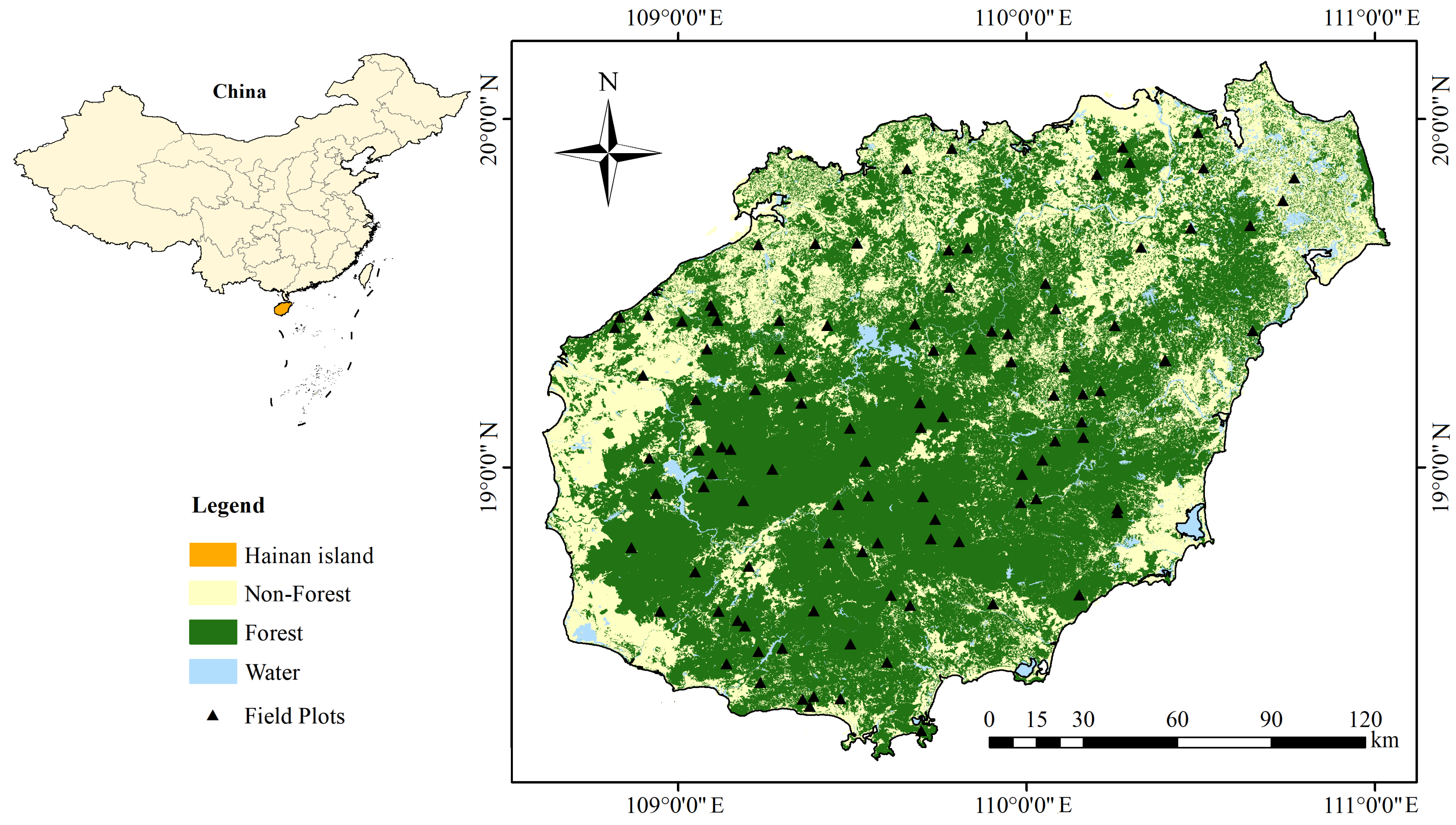
2.1. Study Area

Hainan Island, situated in the northwest of the South China Sea (see Figure 1), encompasses a land area of 33,920 km${}^2$. Its terrain is dome-shaped, with low surrounding areas and a high elevation in the center. The climate in this region is categorized as tropical monsoon, distinguished by abundant sunlight, heat, and precipitation. The average annual temperature ranges from 22 to 27 °C, with an accumulated temperature above 10 °C reaching 8200 °C per year, and an average annual precipitation exceeding 1600 mm [28,29]. The island’s exceptional natural conditions make it the most advantageous region for forestry development in China [28]. Forests cover over 60% of the island’s area [30], including various types such as tropical rainforest, tropical seasonal rainforest, evergreen broad-leaved forest, and coniferous forest [31].

2.2. Data Collection and Preprocessing

2.2.1. GEDI L2A Data

GEDI is a LiDAR satellite system launched by the United States on 5 December 2018. It can observe an area ranging from 51.6°N to 51.6°S [6]. GEDI carries a full-waveform multibeam laser altimeter that carries three laser transmitters, one of which is divided into two beams (coverage beams), and the other two lasers maintain full power (power beams). GEDI produces ground tracks through the dithering of laser beams. Each track consists of circular laser footprints with a distance of 60 m along the track and a diameter of 25 m, with a distance of 600 m between adjacent tracks and a scanning width of $4.2$ km [7].

The GEDI L2A product (version 2) covering Hainan island in 2020 was used in this research. This product provides footprint-level relative height (RH) metrics derived from the received waveform, representing the laser’s energy return height relative to the ground at a specific percentile. For each footprint, we used RH95 as the top canopy height instead of other metrics since RH95 is closest to the ground truth [14]. Due to their reduced penetration capability, coverage beams yield lower canopy height measurement accuracy compared to power beams [6,32]. Thus, only the footprints from the power beam were used in this research. In addition, further quality screening of the GEDI data was performed based on several other data labels, with the thresholds and rationales summarized in

Table 1. Labels, thresholds, and rationales utilized for quality screening of GEDI and ICESat-2 data.

Dataset	Label and Threshold	Rationale
GEDI	degrade_flag = 0	Retaining data that indicates the good status of pointing and positioning information [33].
	quality_flag = 1	Retaining data with valid waveforms [33].
	solar_elevation < 0	Retaining data acquired at night, as the observation precision of daytime data is significantly lower than that of nighttime data [6].
	sensitivity > 0.9	Retaining data with high sensitivity [33].
	2.5 < RH95 < 40	Retaining data within this range is contingent upon field measurement results.
ICESat-2	cloud_flag_atm < 2	Retaining footprints that are less influenced by cloud [34].
	h_canopy_uncertainty = 3.4028235 × 1038	Eliminating data with high measurement uncertainty [34].
	night_flag = 0	Retaining data acquired at night, as the observation precision of daytime data is significantly lower than that of nighttime data [6].
	SNR > 10	Retaining data with high signal-to-noise ratio [10].
	2.5 < h_canopy < 40	Retaining data within this range is contingent upon field measurement results.

.

2.2.2. ICESat-2 ATL08 Data

The ICESat-2 satellite observes between 88°N and 88°S latitude with a 91-day orbital cycle. The Advanced Topographic Laser Altimeter System (ATLAS) carried by the ICESat-2 satellite acquires overlapping ground track footprints at an approximately $0.7$ $\mathrm{m}$ spacing and with a diameter of roughly 14 $\mathrm{m}$. The laser beams emitted are divided into three pairs, where each pair comprises a strong beam and a weak beam, with an energy ratio of 3:1. The separation between each pair in the cross-track direction is approximately $3.3$ km, with a distance of about 90 $\mathrm{m}$ between the strong and weak beams within each pair [35].

The ATL08 vegetation canopy height and surface elevation data product is one of the ICESat-2 products that provides various canopy and topography related metrics for each 14 $\mathrm{m}$ × 100 $\mathrm{m}$ segment along the ground tracks. For this research, we used the ATL08 product (version 5) within the study area throughout 2020, deriving the canopy height metrics h_canopy (98th percentile height relative to the ground) as the top canopy height, as it is the closest to the ground truth [14]. The additional labels employed for data quality screening are presented in Table 1.

After the quality screening, we extracted 30 height-related metrics [10] from ATL08 as the set of explanatory variables for constructing the GIF model, as shown in

Table 2. Metrics used for this study provided by the ICESat-2 ATL08 product.

Metric	Description
latitude	Latitude of each segment center
longitude	Longitude of each segment center
h_canopy	Forest canopy height (98th percentile height)
SNR	Signal-to-noise ratio
canopy_h_metrics	10th, 15th, 20th, 25th, 30th, 35th, 40th, 45th, 50th, 55th, 60th, 65th, 70th, 75th, 80th, 85th, 90th, and 95th percentile height
h_max_canopy	Maximum canopy height
h_mean_canopy	Mean canopy height
h_median_canopy	Median canopy height
h_min_canopy	Minimum canopy height
terrain_slope	Slope of ground
beam_azimuth	Beam azimuth
dem_h	Ground elevation
fvc	Fraction of vegetation coverage

. Additionally, considering that terrain slopes exceeding 10° substantially impact the measurement accuracy of spaceborne LiDAR [36], only GEDI and ICESat-2 data with slopes less than 10° were used in this study.

2.2.3. Sentinel Data

The Sentinel-1 (S-1) satellite carries a C-band synthetic-aperture radar (SAR), with a revisit cycle of up to six days and four imaging modes. In this paper, we selected SAR data in two polarization modes, VH and VV, from the S-1 Interferometric Wide Swath (IW) product. The cloud computing platform Google Earth Engine (GEE) provides 10 m resolution S-1 ground range detected (GRD) images that have undergone thermal noise removal, radiometric calibration, and terrain correction [17]. We utilized this platform to perform the annual median composite of S-1 images for the year 2020 and to extract the study area.

Sentinel-2 (S-2) satellite carries a multispectral imager (MSI) that revisits every five days. It provides 13 bands ranging from visible to short-wave infrared with a spatial resolution of up to 10 m (visible and near-infrared bands) [37]. The GEE platform provides the S-2 level-2A surface reflectance product after atmospheric correction and orthorectification. In this study, we used this product and the cloud probability product provided by GEE to perform cloud removal with a threshold of 50% and annual and monthly median composite to obtain S-2 multispectral images covering the study area in 2020. Temporal features for subsequent analysis were extracted from the monthly normalized difference vegetation index (NDVI) images, which were derived from the monthly S-2 images. These time-series features included the maximum, minimum, mean, and standard deviation of the 2020 temporal NDVI for the study area.

2.2.4. Climate, Terrain, and Land Cover Data

The climate data utilized in this study were obtained from the fifth generation of the reanalysis dataset ERA5 (ECMWF Reanalysis 5), published by the European Centre for Medium-Range Weather Forecasts (ECMWF) [38]. Daily precipitation and temperature data (0.25° resolution) were extracted from the dataset and processed into annual mean precipitation and temperature for the study area from 2000 to 2020 using GEE.

The Shuttle Radar Topography Mission (SRTM) Global 1 arc-second dataset (SRTMGL1) provided by the NASA Jet Propulsion Laboratory (JPL) [39] was used for terrain feature extraction in this research. This product provides digital elevation data with 30 $\mathrm{m}$ resolution on a near-global scale. Elevation data of the study area were collected by clipping on the GEE platform and slope and aspect data were calculated from it.

In this study, non-forest areas of the study area were masked out using the 2020 land cover product GlobeLand30 (V2020). This dataset was produced by the National Geomatics Center of China using Landsat-8, GF-1, HJ-1, and other multispectral data [40]. It possesses a 30 m resolution, categorizing ten land cover classes encompassing forest, with user accuracy for the forest category reaching 87.9% [41].

2.2.5. Field Plot Data

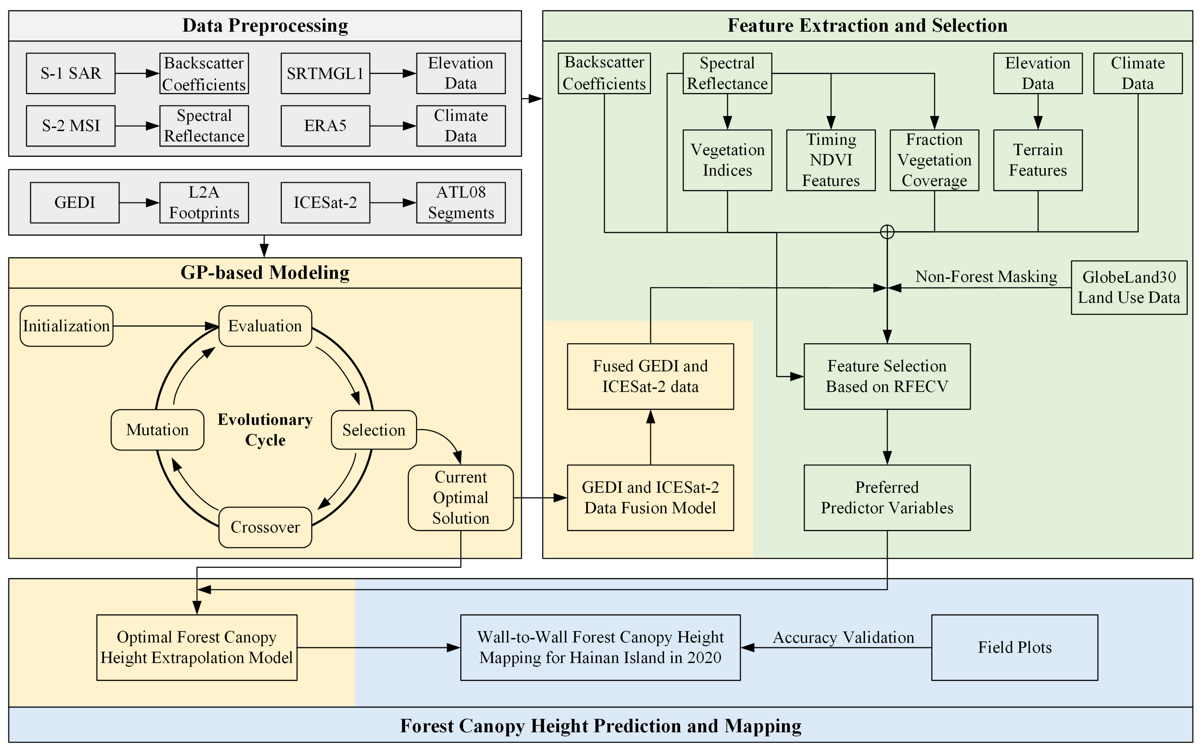
In August 2020, a field survey was conducted, collecting 105 plots measuring 30 $\mathrm{m}$ × 30 $\mathrm{m}$ in size (Figure 1). Within each plot, the canopy height of all individual trees with a diameter at breast height (1.3 m above the ground) greater than 5 cm was measured using a laser rangefinder. Subsequently, the average height of the top 10% of the tallest trees within each plot was calculated and used as the canopy height for that plot. This approach aimed to enhance the representativeness of the measurements, mitigating the influence of individual outliers. We utilized these outcomes as truth data when fitting and evaluating the models in our research. Additionally, the coordinate of the central point of each sample was recorded using a GPS device for the purpose of marking their locations on RS images.

3. Methods

The forest canopy height mapping method proposed in this research entails four stages. Firstly, the multi-source RS data described in Section 2.2 were preprocessed, including preprocessing the data through techniques such as data filtering, image median composite, study area clipping, and resampling to a resolution of 30 $\mathrm{m}$. Secondly, the GP algorithm was employed to construct a GIF model, which was subsequently applied to fuse the GEDI and ICESat-2 data. In the third phase, 33 explanatory variables, categorized into seven classes, were extracted from the preprocessed data. These variables underwent feature filtering through the recursive feature elimination with cross-validation (RFECV) algorithm. Finally, the FCHE model was constructed using the GP algorithm based on the selected explanatory variables and the forest canopy height (response variable) extracted from the fused GEDI and ICESat-2 data. This model was employed to predict and map the forest canopy height continuously in space. The accuracy of the predicted results was validated using field plots. Figure 2 displays the technical flowchart of this method.

3.1. Feature Extraction and Selection

In this research, a total of 33 features across seven categories associated with forest canopy height [4,19,21] were extracted and employed for FCHE model development. Among them, the extraction process of spectral reflectance, backscatter coefficients, timing NDVI features, terrain features, and climate data have been described in Section 2.2. The vegetation indices and fraction of vegetation coverage (FVC) were derived from the multispectral reflectance (details in

Table 3. Explanatory variables extracted from multi-source RS data. B, G, R, NIR, NNIR, RE, and SWIR represent the blue, green, red, near-infrared, narrow near-infrared, red-edge, and short-wave infrared bands of S-2, respectively.

Type	Variable	Description
Spectral reflectance	B, G, R, RE1, RE2, RE3, NIR, NNIR, SWIR1, SWIR2	S-2 2-8, 8A, 11, 12 bands
Vegetation indices	NDVI	(NIR − R)/(NIR + R)
	Enhanced Vegetation Index (EVI)	2.5 × ((NIR − R)/(NIR + 6 × R − 7.5 × B + 1))
	Leaf Area Index (LAI)	3.618 × EVI − 0.118
	Atmospherically Resistant Vegetation Index (ARVI)	((NIR − (2 × R) + B)/(NIR + (2 × R) + B))
	Structure Insensitive Pigment Index (SIPI)	(NIR − B)/(NIR − R)
	Red Edge Chlorophyll Index (RECI)	(RE3/RE1) − 1
	Green Chlorophyll Index (GCI)	(NIR/G) − 1
	Red Green Ratio Index (RGRI)	R/G
	MERIS Terrestrial Chlorophyll Index (MTCI)	(RE2 − RE1)/(RE1 − R)
	Soil Adjust Vegetation Index (SAVI)	(NIR − R) × (1 + 0.5)/(NIR + R + 0.5)
	Difference Vegetation Index (DVI)	NIR-R
Timing NDVI features	Maximum NDVI, minimum NDVI, mean NDVI, stdDev NDVI	Maximum, minimum, mean, and standard deviation of temporal NDVI
Climate data	Precipitation, temperature	Average precipitation and temperature from 2000 to 2020
Terrain features	Elevation, slope, aspect	Elevation, slope and aspect of ground
Backscatter coefficients	VV, VH	Backscattering coefficients values of VV and VH polarization
Biophysical features	Fraction of vegetation coverage (FVC)	Proportion of ground cover by vegetation

).

Feature selection has a pivotal impact on the effectiveness of regression tasks using ML algorithms. It serves to reduce overfitting, computational costs, and model complexity by eliminating irrelevant or redundant features [42]. In this study, we employed the RFECV algorithm for feature selection, which combines the recursive feature elimination (RFE) and cross-validation (CV) techniques. Specifically, RFE utilizes a base model to rank all features based on their importance, followed by the sequential selection of different numbers of features to construct feature subsets. The base model then calculates the average score of all feature subsets for each number of features. The optimal number of features is determined by the number of features corresponding to the highest average score. Finally, this number of features was selected in descending order according to their importance [43]. In this research, we used an RF model, which has demonstrated exceptional regression performance [44], as the base model for RFECV.

3.2. Modeling Based on the GP Algorithm

3.2.1. The GP Algorithm

GP is a global search optimization algorithm developed on the basis of the genetic algorithm. It searches for optimal solutions by simulating the Darwinian process of biological evolution through genetic selection and natural elimination. Due to its strong solving capabilities for nonlinear and complex problems, it has been successfully applied to the study of many problems in geosciences [45]. The fundamental idea of GP is to randomly generate an initial population for a given problem, i.e., a search space. And each individual in the population represents a feasible solution to the problem. Then, each individual’s performance is assessed and the population is optimized iteratively using genetic operations (replication, crossover, and mutation) until the optimal solution or near-optimal solution is found. A more detailed introduction to GP can be found in [46].

In the GP algorithm, an individual is represented by a tree structure consisting of two types of nodes: internal nodes and leaf nodes. Internal nodes, situated within the individual tree, possess at least one child node, denoting functions or operators that combine and manipulate the values of the leaf nodes. Leaf nodes, located at the terminal of the individual tree, lack child nodes and represent constants or variables. For this research, internal nodes and leaf nodes correspond to ML regressors and explanatory variables extracted from RS imagery, respectively. The implementation of GP utilized the third-party Python packages DEAP [47] and TPOT [48].

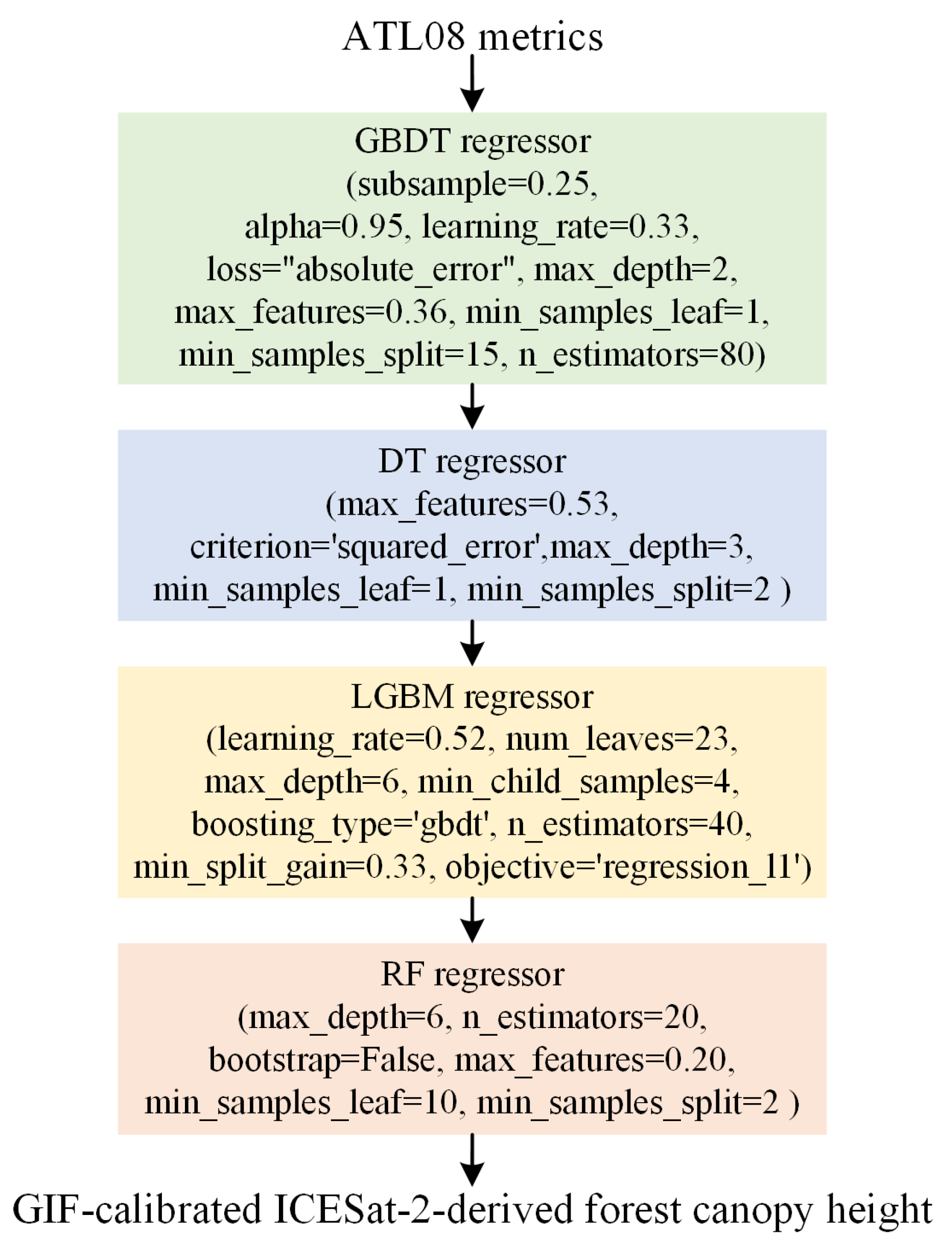
3.2.2. Constructing the GIF Model Based on GP

Given the superior measurement precision of GEDI over ICESat-2 [14], we utilized the forest canopy height derived from the GEDI data (RH95) as the response variable in our study. The ICESat-2 ATL08 metrics in Table 2 were subjected to RFECV screening, and the selected metrics were used as explanatory variables. The GP algorithm was employed to build a GIF model that characterizes the relationship between them.

The data employed for the GIF model fitting are those where the ICESat-2 ATL08 and GEDI L2A data intersect. Specifically, this type of data is determined by whether there was an overlap between the ICESat-2 ATL08 data (segments of 100 m × 14 m) and the GEDI L2A data (circles of 25 m in diameter). These data were split into a training set (70%) and a validation set (30%), randomly.

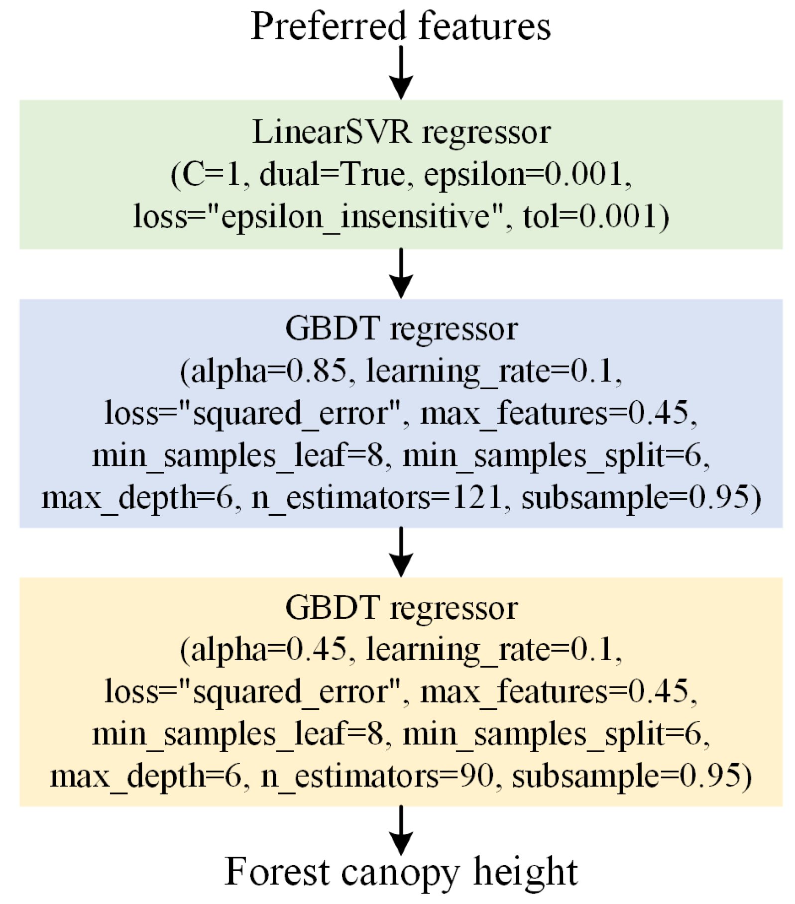
3.2.3. Constructing the FCHE Model Based on GP

The construction of the FCHE model includes three steps. Firstly, the GIF model was employed to fuse the GEDI and ICESat-2 data (hereinafter GIF data). Secondly, 33 image features (Table 3) corresponding to the central locations of the GIF data were extracted, and the preferred features were selected using RFECV. Finally, the GIF-derived forest canopy height and the preferred features were, respectively, taken as the response and explanatory variables, and GP was used to construct the FCHE model based on the GIF data.

Due to the strong generalization ability, proficiency in handling nonlinear problems, and insensitivity to outliers, the RF algorithm has been widely employed for extracting forest-related indicators from RS data [9,21]. In the current study, we devised four experiments to estimate the forest canopy height of Hainan Island for comparative analysis: (1) predicting with RF based on ICESat-2 data; (2) predicting with RF based on GEDI data; (3) predicting with RF based on GIF data; and (4) predicting with the FCHE model constructed using GP based on GIF data. In the comparative trials, RF was optimized through random search for hyperparameter tuning prior to its application.

3.3. Accuracy Evaluation

The root mean squared error (RMSE), the percentage RMSE (pRMSE), and the coefficient of determination (${\mathrm{R}}^2$) were used as accuracy evaluation metrics in this research. Among them, RMSE and pRMSE are used to evaluate the absolute and relative errors of the predicted and true values, respectively. And ${\mathrm{R}}^2$ is employed to assess the goodness of fit of a model. They are calculated as follows:

$$RMSE=\sqrt{\frac{1}{n}\sum _{i=1}^n{(y_i-{\widehat{y}}_i)}^2}$$

(1)

$$pRMSE=\frac{RMSE}{{\overline{y}}_i}\times 100\%$$

(2)

$$R^2=1-\frac{{\sum }_{i=1}^n{\left(y_i-{\widehat{y}}_i\right)}^2}{{\sum }_{i=1}^n{\left(y_i-{\overline{y}}_i\right)}^2}$$

(3)

where $y_i$ and ${\widehat{y}}_i$ represent the actual value and the predicted value for the i-th sample, respectively; $\overline{y}$ indicates the sample mean; and n denotes the total number of samples.

4. Results

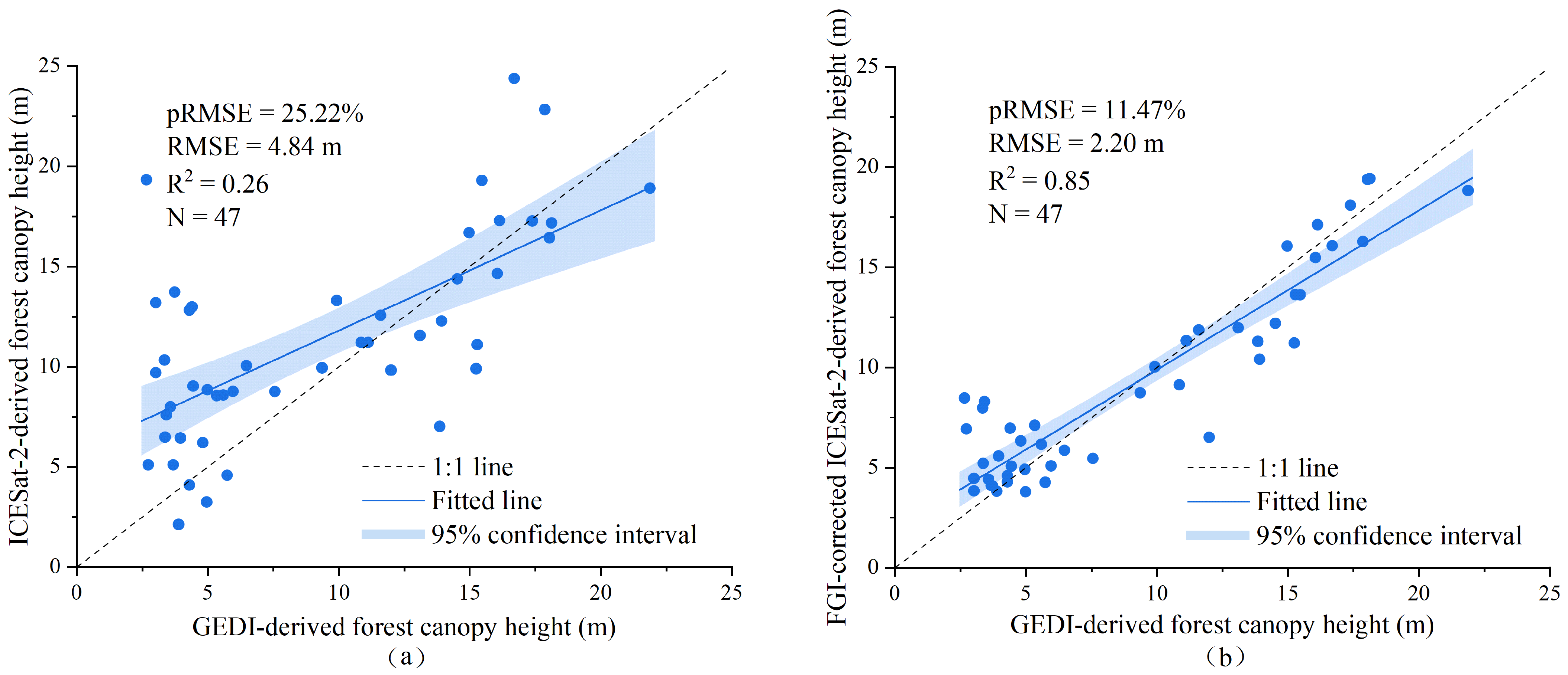
4.1. GIF Model Construction

Following the data quality screening procedures outlined in Section 2.2.1 and Section 2.2.2, a total of 38,971 GEDI L2A footprints and 20,381 ICEsat-2 ATL08 segments were retained. There were 233 pairs of L2A footprints and ATL08 segments with intersections between them (Figure 3), which were utilized to fit the GIF model. These data were randomly split 80%:20% into training and validation sets.

After feature selection, only three canopy height metrics (canopy_h_30th, canopy_h_40th, and canopy_h_50th) were eliminated from the set of ATL08 metrics (Table 2), and the remaining metrics were used as explanatory variables in the construction of the GIF model. The GIF model constructed by GP consists of a sequential arrangement of a gradient-boosting decision tree (GBDT) regressor, decision tree (DT) regressor, light gradient-boosting machine (LGBM) regressor, and RF regressor. The corresponding hyperparameters for the GIF model are presented in Figure 4.

After applying the GIF model to calibrate the forest canopy height derived from ICESat-2 ATL08, a scatterplot (Figure 5) was generated, and three evaluation metrics were computed to facilitate visual comparison of the consistency between the forest height values extracted by ICESat-2 and GEDI before and after calibration.

As shown in Figure 5a, before calibration, the scatterplot exhibited scattered data points with an ${\mathrm{R}}^2$ value of only 0.26, indicating a low level of agreement between them. However, after calibration (Figure 5b), the data points were clearly clustered around the 1:1 reference line and ${\mathrm{R}}^2$ increased to 0.85, while the pRMSE and RMSE values improved by 11.47% and $2.2$ m, respectively. Based on these results, it can be concluded that the consistency between the forest canopy heights extracted from the calibrated ICESat-2 data and those from the GEDI data is significantly higher than that of the uncalibrated ICESat-2 data.

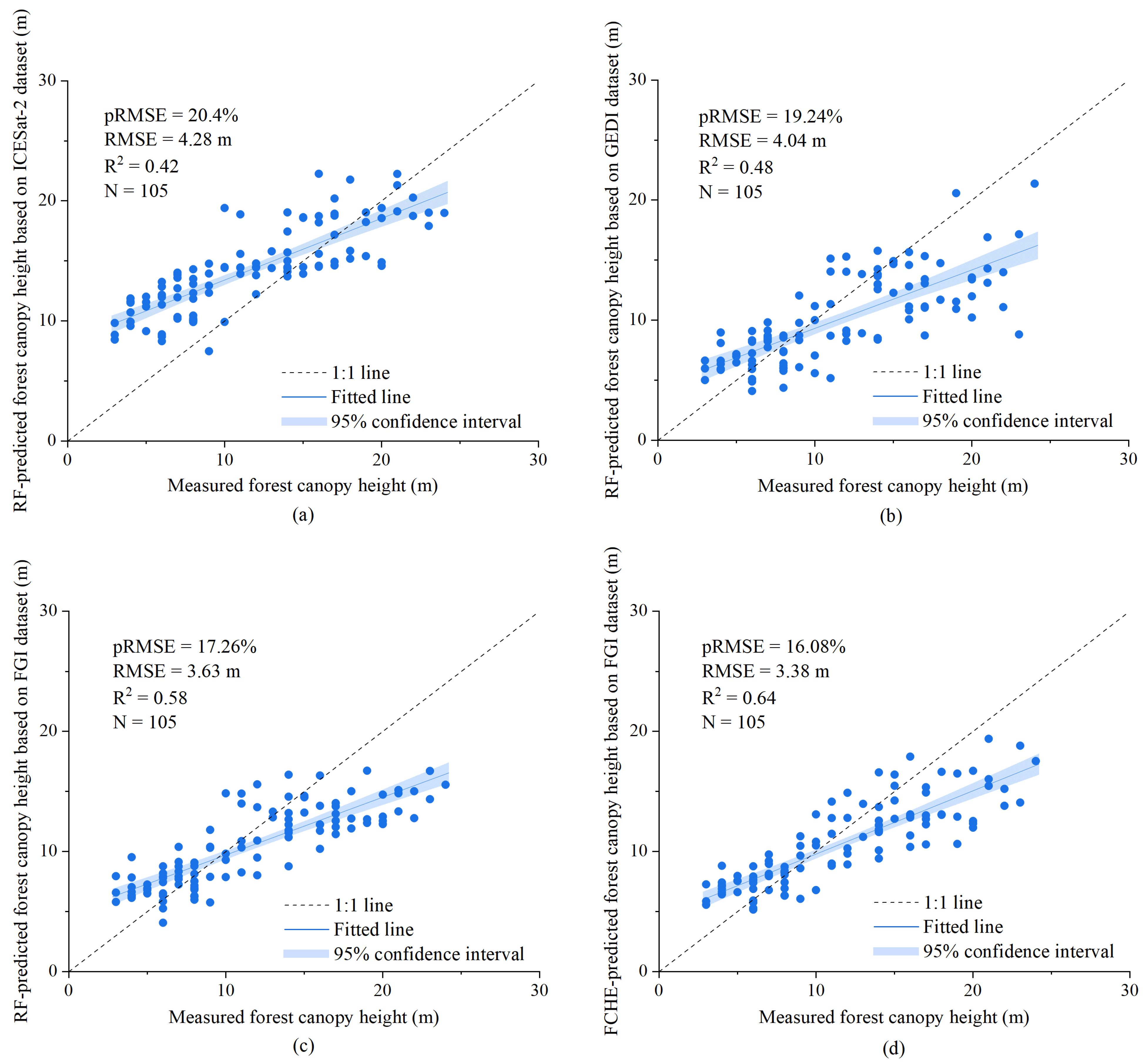
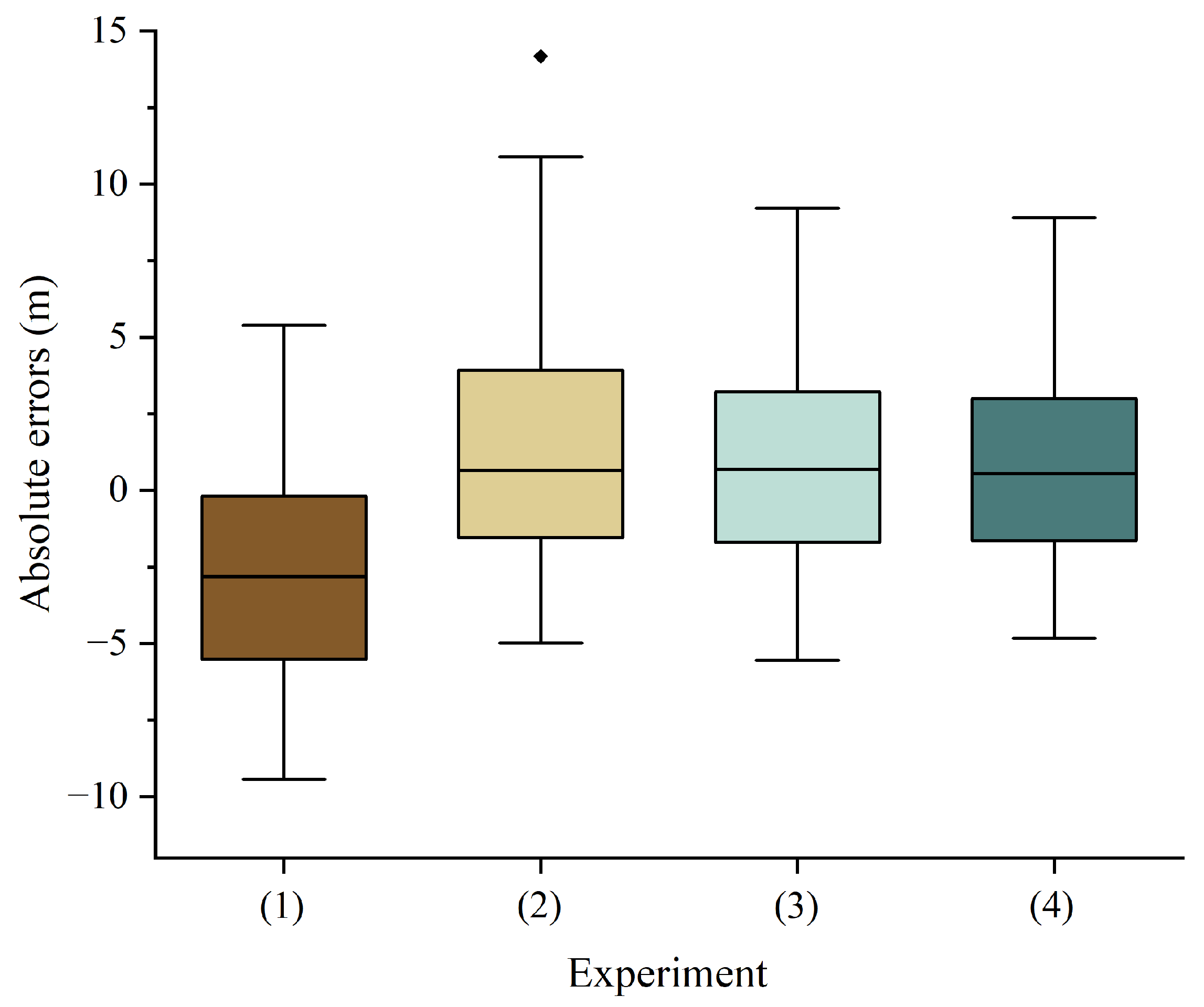
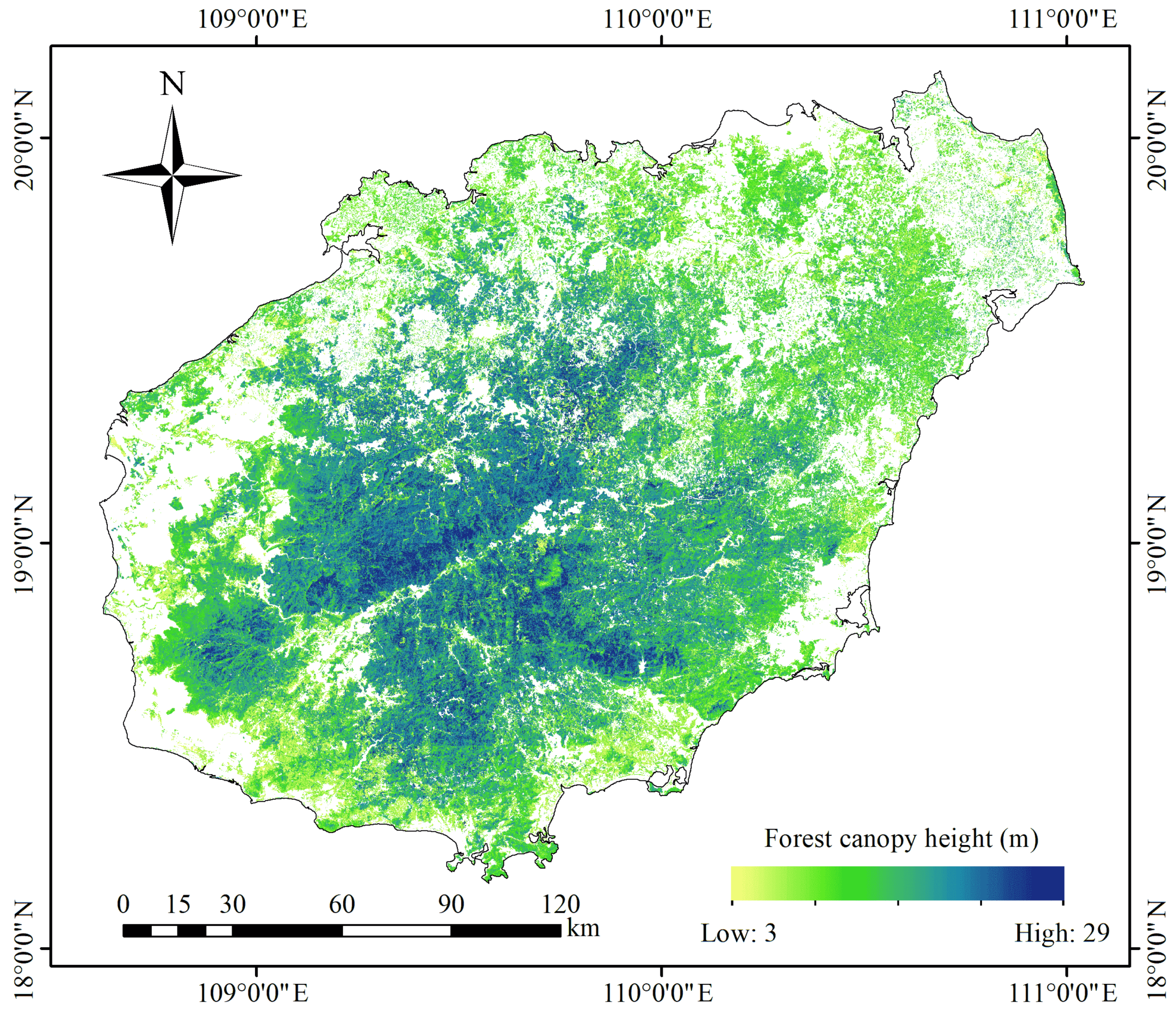
4.2. Forest Canopy Height Prediction, Validation, and Mapping

After conducting feature selection using RFECV, 24, 14, and 17 features were retained from the GEDI, ICESat-2, and GIF datasets, respectively (

Table 4. The image features selected by RFECV.

Dataset	Feature
GEDI	B, G, R, RE1, RE2, NIR, SWIR1, SWIR2, SIPI, RECI, GCI, RGR, MTCI, maximum NDVI, minimum NDVI, mean NDVI, stdDev NDVI, DEM, slope, aspect, temperature, VV, VH, FVC;
ICESat-2	G, R, NIR, SWIR1, SWIR2, MTCI, maximum NDVI, minimum NDVI, mean NDVI, DEM, slope, temperature, VV, VH;
GIF	B, G, R, RE1, NIR, SWIR1, SWIR2, MTCI, maximum NDVI, minimum NDVI, mean NDVI, stdDevNDVI, DEM, slope, aspect, VV, VH

). The results of feature selection across the three datasets exhibited certain similarities, with the retention of multiple spectral bands, most of the terrain features, and both backscatter coefficients from S-1. However, some differences were also noted. The GEDI dataset retained more vegetation indices, while the blue band was excluded in the ICESat-2 dataset. These discrepancies were attributed to differing demands for image information within each dataset.

The FCHE model constructed by GP consisted of a LinearSVR regressor and two GBDT regressors connected in sequence, with the hyperparameters shown in Figure 6. We completed four comparative experiments as outlined in Section 3.2.3, utilizing the RF model optimized through a random search algorithm (see Appendix A-

Table A1. Results of hyperparameter tuning for RF models in three experiments using a random search algorithm.

	Hyperparameter	(1)	(2)	(3)/(4)
Experiment
n_estimators		146	168	167
max_features		19	14	18
min_samples_split		3	2	6
min_samples_leaf		3	5	9
bootstrap		0	0	0
max_depth		19	18	19

for the hyperparameter tuning results), and the FCHE model developed by GP. The results of accuracy validation for these experiments are presented in Figure 7.

According to Figure 7, experiment (4) achieved the highest ${\mathrm{R}}^2$ of 0.64, the lowest RMSE of $3.38$ $\mathrm{m}$, and the lowest pRMSE of 16.08% among all four experiments. Experiment (3) also performed well, with an ${\mathrm{R}}^2$ of 0.58, an RMSE of $3.63$ $\mathrm{m}$, and a pRMSE of 17.26%. In contrast, experiments (1) and (2) had lower ${\mathrm{R}}^2$ and higher RMSE and pRMSE values, indicating poor performance. Overall, the accuracy validation results indicated that experiment (4), which utilized the FCHE model based on GIF data to predict forest canopy height, performed the best.

To further compare the predictive performance of the four experiments on forest canopy height, we generated boxplots of the absolute errors (difference between true and predicted values, AE) in their predictions (Figure 8). From this figure, it can be observed that the median AEs of experiments (2), (3), and (4) are relatively close to zero, while experiment (1) is around $-2.5$ $\mathrm{m}$. In terms of the distribution of AE, experiment (1) predominantly ranges from −10 $\mathrm{m}$ to 5 $\mathrm{m}$, whereas the other three experiments generally fall within the range of −5 $\mathrm{m}$ to 10 $\mathrm{m}$. Nonetheless, differences persist among the latter three. Experiment (2) exhibits a notably higher upper extreme and upper quartile compared to (3) and (4), while its lower extreme and lower quartile are closer to (4) and higher than (3). However, experiment (2) is the only one among the four with outliers. Overall, experiment (4), which involves predicting forest canopy height using the FCHE model based on GIF data, demonstrates the lowest predictive error. Experiments (2) and (3) slightly lag behind (4), while experiment (1) exhibits the poorest predictive performance.

Given the optimal results obtained from experiment (4), a forest canopy height map of Hainan Island in 2020 with a resolution of 30 $\mathrm{m}$ was generated using its predicted results, as illustrated in Figure 9. The outcomes demonstrate notable regional characteristics of the forest height on Hainan Island. Specifically, forests located in the northeast and coastal areas of the island generally have shorter heights, while those in the central and southwestern regions tend to exceed 20 $\mathrm{m}$ in height.

5. Discussion

5.1. Advantages of the Proposed Forest Canopy Height Prediction Method

As a crucial ecological indicator of forests, precise measurement of forest canopy height is vital for evaluating forest carbon storage, conducting ecological research, and evaluating the economic value of forests [12,19]. Considering the shortcomings in existing research utilizing spaceborne LiDAR data for wall-to-wall forest canopy height prediction, we proposed a method in this study. Guided by the GP algorithm, we integrated LiDAR satellites with Sentinel-1/2, terrain, and climate data to generate a forest canopy height map at a 30 m resolution. Leveraging the outstanding modeling performance of GP, our study established two key models, namely, GIF and FCHE, enabling the successful fusion of the GEDI and ICESat-2 data and achieving wall-to-wall predictions of forest canopy height. And the accurate estimation results attest to the effectiveness of this technique. Compared to conventional methods, our approach offers the following advantages.

Firstly, our method enables the synergistic usage of the GEDI and ICESat-2 data for forest height prediction. Typically, due to differences in the operational modes of these two LiDAR systems, there exists measurement bias for observations of the same location, precluding the direct combined usage of these two datasets for analysis [14,36]. Nevertheless, using only one LiDAR dataset as the sole source of ground samples for regression can result in strong strip effects and adversely affect prediction accuracy due to the distribution of LiDAR footprints along the ground trajectories rather than at random [7]. To address this issue, we constructed a GIF model using the GP algorithm with the GEDI-derived height as the response variable and multiple ICESat-2 metrics as explanatory variables. This approach enables the combining of the ICESat-2 and GEDI data, facilitating their collaborative use in research. With the incorporation of additional ground samples, our approach overcomes strip effects and improves the GP algorithm’s ability to comprehend data features, resulting in superior performance models and enhanced prediction accuracy. As shown in the accuracy assessment results (Figure 7a–c), the collaborative use of the ICESat-2 and GEDI data within the same regressor significantly enhances the accuracy of forest canopy height prediction compared to using either dataset alone.

Moreover, our method can autonomously construct an optimal FCHE model based on explanatory variables. In existing research, predicting forest height is commonly achieved by directly using a well-performing model, such as an RF regressor [4,18,49]. However, it is worth noting that when confronted with different explanatory variables, the same regressor exhibits varying performance. Therefore, empirically specifying a model cannot guarantee optimal performance in the current task. Moreover, the performance of a single regressor is typically inferior to that of an ensemble model composed of multiple regressors, especially when dealing with datasets containing complex features [50]. In this study, we constructed an FCHE model using GP based on the explanatory variables, which is a stacking ensemble model consisting of one LinearSVR and two GBDT regressors. According to the results of accuracy verification (Figure 7c,d), using the same explanatory variables, the FCHE model constructed based on GP improved the pRMSE, RMSE, and ${\mathrm{R}}^2$ by 1.18%, $0.25$ $\mathrm{m}$, and 0.06, respectively, compared to the RF regressor tuned by the random search algorithm. These results illustrate that using GP to construct the FCHE model is beneficial for improving forest canopy height prediction accuracy.

Lastly, our method exhibits high transferability. It comprises two main components: constructing the GIF model to perform calibration from ICESat-2 ATL08 data to GEDI L2A data and developing the FCHE model for wall-to-wall forest height prediction. Each model includes multiple regressors and numerous hyperparameters. Such complex models, when directly applied to other study areas, often underperform due to their inability to adapt to new data [51,52]. In contrast, for this research, both the GIF and FCHE models were autonomously constructed using the GP algorithm based on explanatory variables, eliminating the need for manual intervention. This enables the application of this method in other research areas, where GP can construct new, well-performing GIF and FCHE models tailored to new sets of explanatory variables, thus maintaining robust predictive accuracy. Furthermore, the spaceborne LiDAR data and RS images employed in this study are openly available, further enhancing the transferability of our method.

5.2. Limitations and Potential Refinements

Although the proposed method offers three advantages, as mentioned above, several shortcomings must be considered. Firstly, after filtering out low-quality data points, only 233 intersection points were identified from approximately 40,000 GEDI footprints and 20,000 ICESat-2 segments covering Hainan Island (33,920 km${}^2$). This implies that it may be challenging to identify sufficient intersection points for constructing the GIF model in smaller study areas. Slope correction of LiDAR data can mitigate this issue to some extent. As the topographic relief can affect the accuracy of LiDAR measurements of forest height by changing the position and direction of LiDAR through the canopy, we excluded all GEDI and ICESat-2 data located at slopes greater than 10°, as suggested by existing studies [10]. However, it is possible that a fraction of the excluded LiDAR data could be regained through precise slope correction [53,54]. Future studies will explore accurate slope corrections for ICESat-2 and GEDI data to obtain more LiDAR data.

Secondly, in this research, although there were multiple forest types on Hainan Island [31], we did not develop separate GIF and FCHE models for each category due to the limited number of intersection points between GEDI and ICESat-2 data. Nevertheless, it is noteworthy that the accuracy of spaceborne LiDAR measurements can vary depending on the forest category due to differences in forest structure [14]. Therefore, we will try to explore the extent to which forest categories affect the accuracy of forest height predictions using this approach in a future study. This could be achieved by selecting a larger study area or conducting slope correction on LiDAR data to obtain more intersection points.

Finally, the inconsistent spatial resolutions of the RS data used in this study may have an adverse effect on the accuracy of the forest canopy height predictions. For the explanatory variables, the original raw RS data consisted of multiple resolutions, including at 10 $\mathrm{m}$, 30 $\mathrm{m}$, etc. After comprehensively considering the differences between data resolutions and computational resources required, we decided to resample all bands to 30 $\mathrm{m}$ resolution before estimating the forest canopy height. This allows us to provide relatively high resolution tree height estimation results while consuming fewer computational resources and storage space, thus enhancing the prediction efficiency. However, the resampling of the independent variables may result in information loss, which could detrimentally affect the accuracy of forest height estimation. Regarding the response variable, the forest canopy height data extracted from GEDI and ICESat-2 have spatial resolutions of 25 $\mathrm{m}$ and 14 $\mathrm{m}$ × 100 $\mathrm{m}$, respectively. Although the latter differed substantially from 30 $\mathrm{m}$, in this study, we employed the GIF model to calibrate the latter to the former, achieving excellent results (RMSE = $2.2$ $\mathrm{m}$, ${\mathrm{R}}^2$ = 0.85). Consequently, we consider the calibrated ICESat-2 data to exhibit a resolution close to 25 $\mathrm{m}$ rather than 100 m × 14 m. However, there still exists a resolution disparity between the response and explanatory variables, which may have an unfavorable impact on the estimation accuracy of our method. Nevertheless, despite this discrepancy, our accuracy validation using field-measured tree height data reveals that the precision of this method for estimating forest canopy height remains satisfactory (RMSE = $3.38$ $\mathrm{m}$, ${\mathrm{R}}^2$ = 0.64). This outcome can provide valuable insights for research related to predicting forest canopy height using multi-source RS data.

6. Conclusions

For this research, we proposed an innovative method to map forest canopy height at a 30-m resolution by combining the ICESat-2 and GEDI LiDAR data with Sentinel-1/2, terrain, and climate data guided by GP. Our main conclusions are as follows: (1) After being calibrated by the GIF model constructed by GP, GEDI and ICESat-2 measured forest canopy height showed good agreement, with a pRMSE, RMSE, and ${\mathrm{R}}^2$ of 11.47%, $2.2$ m, and 0.85, respectively. This result demonstrates the potential of GP in constructing wellperforming GIF models. (2) The prediction accuracy based on the GIF data was significantly higher than that based solely on the GEDI or ICESat-2 data, validating the value of using both datasets to improve prediction accuracy under the same regression model. (3) The FCHE model constructed using GP showed an improvement of 1.18%, $0.25$ m, and 0.06 in pRMSE, RMSE, and ${\mathrm{R}}^2$, respectively, compared to the predictive results obtained by RF. This improvement highlights the advantage of using GP in constructing FCHE models. (4) The final accuracy of our method based on field plots was 0.64, $3.38$ $\mathrm{m}$, and 16.08% for ${\mathrm{R}}^2$, RMSE, and pRMSE, respectively, confirming the reliability of our proposed 30 m large-scale forest canopy height mapping method. (5) As the GIF and FCHE models in this study were autonomously constructed by GP based on the explanatory variables without any manual intervention, we consider that our method has high transferability and can achieve satisfactory results when applied to new study areas. In summary, the high accuracy and transferability of our method allow for accurate mapping of forest canopy height in other study areas, thereby providing valuable data support for understanding forest ecosystem structure and function, as well as for forest management and conservation.

References

1. Lang, N.; Kalischek, N.; Armston, J.; Schindler, K.; Dubayah, R.; Wegner, J.D. Global canopy height regression and uncertainty estimation from GEDI LIDAR waveforms with deep ensembles. Remote Sens. Environ. 2022, 268, 112760. [Google Scholar] [CrossRef]
2. Coops, N.C.; Tompalski, P.; Goodbody, T.R.; Queinnec, M.; Luther, J.E.; Bolton, D.K.; White, J.C.; Wulder, M.A.; van Lier, O.R.; Hermosilla, T. Modelling lidar-derived estimates of forest attributes over space and time: A review of approaches and future trends. Remote Sens. Environ. 2021, 260, 112477. [Google Scholar] [CrossRef]
3. Huang, X.; Cheng, F.; Wang, J.; Duan, P.; Wang, J. Forest Canopy Height Extraction Method Based on ICESat-2/ATLAS Data. IEEE Trans. Geosci. Remote Sens. 2023, 61, 5700814. [Google Scholar] [CrossRef]
4. Zhu, X.; Wang, C.; Nie, S.; Pan, F.; Xi, X.; Hu, Z. Mapping forest height using photon-counting LiDAR data and Landsat 8 OLI data: A case study in Virginia and North Carolina, USA. Ecol. Ind. 2020, 114, 106287. [Google Scholar] [CrossRef]
5. Li, W.; Niu, Z.; Shang, R.; Qin, Y.; Wang, L.; Chen, H. High-resolution mapping of forest canopy height using machine learning by coupling ICESat-2 LiDAR with Sentinel-1, Sentinel-2 and Landsat-8 data. Int. J. Appl. Earth Obs. Geoinf. 2020, 92, 102163. [Google Scholar] [CrossRef]
6. Potapov, P.; Li, X.; Hernandez-Serna, A.; Tyukavina, A.; Hansen, M.C.; Kommareddy, A.; Pickens, A.; Turubanova, S.; Tang, H.; Silva, C.E.; et al. Mapping global forest canopy height through integration of GEDI and Landsat data. Remote Sens. Environ. 2021, 253, 112165. [Google Scholar] [CrossRef]
7. Liu, X.; Su, Y.; Hu, T.; Yang, Q.; Liu, B.; Deng, Y.; Tang, H.; Tang, Z.; Fang, J.; Guo, Q. Neural network guided interpolation for mapping canopy height of China’s forests by integrating GEDI and ICESat-2 data. Remote Sens. Environ. 2022, 269, 112844. [Google Scholar] [CrossRef]
8. Yamamoto, Y.; Matsumoto, K. The effect of forest certification on conservation and sustainable forest management. J. Clean. Prod. 2022, 363, 132374. [Google Scholar] [CrossRef]
9. Huang, W.; Min, W.; Ding, J.; Liu, Y.; Hu, Y.; Ni, W.; Shen, H. Forest height mapping using inventory and multi-source satellite data over Hunan Province in southern China. For. Ecosyst. 2022, 9, 100006. [Google Scholar] [CrossRef]
10. Zhu, X. Forest Height Retrieval of China with a Resolution of 30 m Using ICESat-2 and GEDI Data. Ph.D. Thesis, University of Chinese Academy of Sciences, Beijing, China, 2021. [Google Scholar]
11. Wallner, A.; Friedrich, S.; Geier, E.; Meder-Hokamp, C.; Wei, Z.; Kindu, M.; Tian, J.; Döllerer, M.; Schneider, T.; Knoke, T. A remote sensing-guided forest inventory concept using multispectral 3D and height information from ZiYuan-3 satellite data. Forestry 2022, 95, 331–346. [Google Scholar] [CrossRef]
12. Wang, Y.; Zhang, X.; Guo, Z. Estimation of tree height and aboveground biomass of coniferous forests in North China using stereo ZY-3, multispectral Sentinel-2, and DEM data. Ecol. Ind. 2021, 126, 107645. [Google Scholar] [CrossRef]
13. Guo, Q.; Su, Y.; Hu, T.; Guan, H.; Jin, S.; Zhang, J.; Zhao, X.; Xu, K.; Wei, D.; Kelly, M.; et al. Lidar boosts 3D ecological observations and modelings: A review and perspective. IEEE Geosci. Remote Sens. Mag. 2020, 9, 232–257. [Google Scholar] [CrossRef]
14. Zhu, X.; Nie, S.; Wang, C.; Xi, X.; Lao, J.; Li, D. Consistency analysis of forest height retrievals between GEDI and ICESat-2. Remote Sens. Environ. 2022, 281, 113244. [Google Scholar] [CrossRef]
15. Zhou, X.; Li, C. Mapping the vertical forest structure in a large subtropical region using airborne LiDAR data. Ecol. Ind. 2023, 154, 110731. [Google Scholar] [CrossRef]
16. Jiang, F.; Zhao, F.; Ma, K.; Li, D.; Sun, H. Mapping the forest canopy height in Northern China by synergizing ICESat-2 with Sentinel-2 using a stacking algorithm. Remote Sens. 2021, 13, 1535. [Google Scholar] [CrossRef]
17. Kacic, P.; Hirner, A.; Da Ponte, E. Fusing Sentinel-1 and-2 to Model GEDI-Derived Vegetation Structure Characteristics in GEE for the Paraguayan Chaco. Remote Sens. 2021, 13, 5105. [Google Scholar] [CrossRef]
18. Liao, Z.; Van Dijk, A.I.; He, B.; Larraondo, P.R.; Scarth, P.F. Woody vegetation cover, height and biomass at 25-m resolution across Australia derived from multiple site, airborne and satellite observations. Int. J. Appl. Earth Obs. Geoinf. 2020, 93, 102209. [Google Scholar] [CrossRef]
19. Xi, Z.; Xu, H.; Xing, Y.; Gong, W.; Chen, G.; Yang, S. Forest canopy height mapping by synergizing icesat-2, sentinel-1, sentinel-2 and topographic information based on machine learning methods. Remote Sens. 2022, 14, 364. [Google Scholar] [CrossRef]
20. Wang, X.; Cheng, X.; Gong, P.; Huang, H.; Li, Z.; Li, X. Earth science applications of ICESat/GLAS: A review. Int. J. Remote Sens. 2011, 32, 8837–8864. [Google Scholar] [CrossRef]
21. Chen, L.; Ren, C.; Zhang, B.; Wang, Z.; Liu, M.; Man, W.; Liu, J. Improved estimation of forest stand volume by the integration of GEDI LiDAR data and multi-sensor imagery in the Changbai Mountains Mixed forests Ecoregion (CMMFE), northeast China. Int. J. Appl. Earth Obs. Geoinf. 2021, 100, 102326. [Google Scholar] [CrossRef]
22. Nandy, S.; Srinet, R.; Padalia, H. Mapping forest height and aboveground biomass by integrating ICESat-2, Sentinel-1 and Sentinel-2 data using Random Forest algorithm in northwest Himalayan foothills of India. Geophys. Res. Lett. 2021, 48, e2021GL093799. [Google Scholar] [CrossRef]
23. Pourshamsi, M.; Xia, J.; Yokoya, N.; Garcia, M.; Lavalle, M.; Pottier, E.; Balzter, H. Tropical forest canopy height estimation from combined polarimetric SAR and LiDAR using machine-learning. ISPRS J. Photogramm. Remote Sens. 2021, 172, 79–94. [Google Scholar] [CrossRef]
24. Liu, C.; Lyu, W.; Zhao, W.; Zheng, F.; Lu, J. Exploratory research on influential factors of China’s sulfur dioxide emission based on symbolic regression. Environ. Monit. Assess. 2023, 195, 41. [Google Scholar] [CrossRef] [PubMed]
25. Niu, G.; Yi, X.; Chen, C.; Li, X.; Han, D.; Yan, B.; Huang, M.; Ying, G. A novel effluent quality predicting model based on genetic-deep belief network algorithm for cleaner production in a full-scale paper-making wastewater treatment. J. Clean. Prod. 2020, 265, 121787. [Google Scholar] [CrossRef]
26. Asadzadeh, M.Z.; Gänser, H.P.; Mücke, M. Symbolic regression based hybrid semiparametric modelling of processes: An example case of a bending process. Appl. Eng. Sci. 2021, 6, 100049. [Google Scholar] [CrossRef]
27. Kommenda, M.; Burlacu, B.; Kronberger, G.; Affenzeller, M. Parameter identification for symbolic regression using nonlinear least squares. Genet. Program. Evolvable Mach. 2020, 21, 471–501. [Google Scholar] [CrossRef]
28. Wang, X.; Wang, X.; Zhu, M.; Wang, W.; Liang, Q.; Zou, Y.; Li, C.; Tang, P.; Ren, H. Carbon storage and economic assessment of the main forest types vegetation in Hainan. J. Cent. South Univ. Forest. Technol. 2017, 37, 92–98. [Google Scholar]
29. Chen, Y. Risk Assessment of Typhoon Disaster in Hainan Island Based on GIS. Master’s Thesis, Chongqing Jiaotong University, Chongqing, China, 2021. [Google Scholar]
30. Han, G.; Chen, J.; He, C.; Li, S.; Wu, H.; Liao, A.; Peng, S. A web-based system for supporting global land cover data production. ISPRS J. Photogramm. Remote Sens. 2015, 103, 66–80. [Google Scholar] [CrossRef]
31. Gu, X.; Chen, B.; Ting, Y.; Guangyang, L.; Zhixiang, W.; Weili, K. Spatio-temporal Changes of Forest in Hainan Island from 2007 to 2018 Based on Multi-source Remote Sensing Data. Chin. J. Trop. Crops 2022, 43, 418–429. [Google Scholar]
32. Beck, J.; Wirt, B.; Armston, J.; Hofton, M.; Luthcke, S.; Tang, H. Global Ecosystem Dynamics Investigation (GEDI) Level 02 User Guide. Doc. Version 2021, 2, 14–15. [Google Scholar]
33. Dubayah, R.; Hofton, M.; Blair, J.B.; Armston, J.; Tang, H.; Luthcke, S. GEDI L2A Elevation and Height Metrics Data Global Footprint Level V002. 2021. Available online: https://lpdaac.usgs.gov/products/gedi02_av002/ (accessed on 14 August 2022).
34. Neuenschwander, A.L.; Pitts, K.L.; Jelley, B.P.; Robbins, J.; Klotz, B.; Popescu, S.C.; Nelson, R.F.; Harding, D.; Pederson, D.; Sheridan, R. ATLAS/ICESat-2 L3A Land and Vegetation Height, Version 5. 2021. Available online: https://nsidc.org/data/atl08/versions/5 (accessed on 19 July 2022).
35. Zhang, J.; Tian, J.; Li, X.; Wang, L.; Chen, B.; Gong, H.; Ni, R.; Zhou, B.; Yang, C. Leaf area index retrieval with ICESat-2 photon counting LiDAR. Int. J. Appl. Earth Obs. Geoinf. 2021, 103, 102488. [Google Scholar] [CrossRef]
36. Liu, A.; Cheng, X.; Chen, Z. Performance evaluation of GEDI and ICESat-2 laser altimeter data for terrain and canopy height retrievals. Remote Sens. Environ. 2021, 264, 112571. [Google Scholar] [CrossRef]
37. Drusch, M.; Del Bello, U.; Carlier, S.; Colin, O.; Fernandez, V.; Gascon, F.; Hoersch, B.; Isola, C.; Laberinti, P.; Martimort, P.; et al. Sentinel-2: ESA’s optical high-resolution mission for GMES operational services. Remote Sens. Environ. 2012, 120, 25–36. [Google Scholar] [CrossRef]
38. Hersbach, H.; Bell, B.; Berrisford, P.; Hirahara, S.; Horányi, A.; Muñoz-Sabater, J.; Nicolas, J.; Peubey, C.; Radu, R.; Schepers, D.; et al. The ERA5 global reanalysis. Quart. J. Roy. Meteor. Soc. 2020, 146, 1999–2049. [Google Scholar] [CrossRef]
39. Farr, T.G.; Rosen, P.A.; Caro, E.; Crippen, R.; Duren, R.; Hensley, S.; Kobrick, M.; Paller, M.; Rodriguez, E.; Roth, L.; et al. The shuttle radar topography mission. Rev. Geophys. 2007, 45, 1–23. [Google Scholar] [CrossRef]
40. Jun, C.; Ban, Y.; Li, S. Open access to Earth land-cover map. Nature 2014, 514, 434. [Google Scholar] [CrossRef] [PubMed]
41. Chen, J.; Chen, L.; Chen, F.; Ban, Y.; Li, S.; Han, G.; Tong, X.; Liu, C.; Stamenova, V.; Stamenov, S. Collaborative validation of GlobeLand30: Methodology and practices. Geo-Spat. Inf. Sci. 2021, 24, 134–144. [Google Scholar] [CrossRef]
42. Miao, J.; Niu, L. A survey on feature selection. Procedia Comput. Sci. 2016, 91, 919–926. [Google Scholar] [CrossRef]
43. Xing, H.; Niu, J.; Feng, Y.; Hou, D.; Wang, Y.; Wang, Z. A coastal wetlands mapping approach of Yellow River Delta with a hierarchical classification and optimal feature selection framework. CATENA 2023, 223, 106897. [Google Scholar] [CrossRef]
44. Huang, H.; Liu, C.; Wang, X.; Biging, G.S.; Chen, Y.; Yang, J.; Gong, P. Mapping vegetation heights in China using slope correction ICESat data, SRTM, MODIS-derived and climate data. ISPRS J. Photogramm. Remote Sens. 2017, 129, 189–199. [Google Scholar] [CrossRef]
45. Lary, D.J.; Alavi, A.H.; Gandomi, A.H.; Walker, A.L. Machine learning in geosciences and remote sensing. Geosci. Front. 2016, 7, 3–10. [Google Scholar] [CrossRef]
46. Koza, J.R. Genetic programming as a means for programming computers by natural selection. Stat. Comput. 1994, 4, 87–112. [Google Scholar] [CrossRef]
47. Fortin, F.A.; De Rainville, F.M.; Gardner, M.A.G.; Parizeau, M.; Gagné, C. DEAP: Evolutionary algorithms made easy. J. Mach. Learn Res. 2012, 13, 2171–2175. [Google Scholar]
48. Olson, R.S.; Moore, J.H. TPOT: A tree-based pipeline optimization tool for automating machine learning. In Proceedings of the Workshop on Automatic Machine Learning; PMLR: New York, NY, USA, 2016; pp. 66–74. [Google Scholar]
49. Rahman, M.F.; Onoda, Y.; Kitajima, K. Forest canopy height variation in relation to topography and forest types in central Japan with LiDAR. For. Ecol. Manag. 2022, 503, 119792. [Google Scholar] [CrossRef]
50. Le, T.T.; Fu, W.; Moore, J.H. Scaling tree-based automated machine learning to biomedical big data with a feature set selector. Bioinformatics 2020, 36, 250–256. [Google Scholar] [CrossRef]
51. Long, M.; Zhu, H.; Wang, J.; Jordan, M.I. Deep transfer learning with joint adaptation networks. In Proceedings of the International Conference on Machine Learning; PMLR: New York, NY, USA, 2017; pp. 2208–2217. [Google Scholar]
52. Tan, C.; Sun, F.; Kong, T.; Zhang, W.; Yang, C.; Liu, C. A survey on deep transfer learning. In Proceedings of the Artificial Neural Networks and Machine Learning–ICANN 2018: 27th International Conference on Artificial Neural Networks, Rhodes, Greece, 4–7 October 2018; Proceedings, Part III 27. Springer: Cham, Switzerland, 2018; pp. 270–279. [Google Scholar]
53. Ni, W.; Zhang, Z.; Sun, G. Assessment of slope-adaptive metrics of GEDI waveforms for estimations of forest aboveground biomass over mountainous areas. J. Remote Sens. 2021, 2021, 9805364. [Google Scholar] [CrossRef]
54. Li, B.; Zhao, T.; Su, X.; Fan, G.; Zhang, W.; Deng, Z.; Yu, Y. Correction of Terrain Effects on Forest Canopy Height Estimation Using ICESat-2 and High Spatial Resolution Images. Remote Sens. 2022, 14, 4453. [Google Scholar] [CrossRef]
Figure 1. Location, forest cover, and field plots in the study area.
Remotesensing 16 00110 g001
Figure 2. Technical roadmap of this method.
Remotesensing 16 00110 g002
Figure 3. Quality-screened GEDI and ICESat-2 data and their intersection points.
Remotesensing 16 00110 g003
Figure 4. The GIF model constructed using GP.
Remotesensing 16 00110 g004
Figure 5. Scatterplots of GEDI-derived forest canopy height against raw ICESat-2-derived forest canopy height (a), and GIF-calibrated ICESat-2-derived forest canopy height (b).
Remotesensing 16 00110 g005
Figure 6. The FCHE model constructed by GP.
Remotesensing 16 00110 g006
Figure 7. Scatterplots of field-measured forest canopy heights versus the forest canopy heights predicted by four contrast experiments: (a) predicting with RF based on ICESat-2 data, (b) predicting with RF based on GEDI data, (c) predicting with RF based on GIF data, and (d) predicting with the FCHE model constructed by GP based on GIF data.
Remotesensing 16 00110 g007
Figure 8. Boxplots of absolute errors from four experiments.
Remotesensing 16 00110 g008
Figure 9. Predicted forest canopy height of Hainan Island using the FCHE model constructed by GP with GIF data.
Remotesensing 16 00110 g009