Abstract
Hyperspectral image (HSIs) denoising is a preprocessing step that plays a crucial role in many applications used in Earth observation missions. Low-rank tensor representation can be utilized to restore mixed-noise HSIs, such as those affected by mixed Gaussian, impulse, stripe, and deadline noises. Although there is a considerable body of research on spatial and spectral prior knowledge concerning subspace, the correlation between the spectral continuity and the nonlocal sparsity of the spectral and spatial factors is not yet fully understood. To address this deficiency, in the present study, we determined the correlation between these factors using a cascaded technique, and we describe in this paper the double-factor tensor cascaded-rank (DFTCR) minimization method that was used. The information existing in the nonlocal sparsity property of the spatial factor was employed to promote a geometrical feature representation, and a tensor cascaded-rank minimization approach was introduced as a nonlocal self-similarity to promote restoration quality. The continuity between the difference and nonlocal gradient sparsity constraints of the spectral factor was also introduced to learn the basis. Furthermore, to estimate the solutions of the proposed model, we developed an algorithm based on the alternating direction method of multipliers (ADMM). The performance of the DFTCR method was tested by a comparison with eleven established denoising methods for HSIs. The results showed that the proposed DFTCR method exhibited superior performance in the removal of mixed noise from HSIs.
1. Introduction
Hyperspectral images (HSIs), with detailed spatial and spectral information containing hundreds of contiguous spectral bands, are used for agricultural [1] and military [2] purposes, as well as for disaster monitoring [3,4], terrain detection [5], ecological protection [6], and land use analysis [7]. The successful use of such applications is guaranteed by the use of high-quality HSIs [8,9]. However, image quality may be degraded by noise, which impedes the development of subsequent applications, including classification, unmixing, fusion, and target detection. Because hardware-based noise suppression solutions involve considerable maintenance and renewal costs [10], the development of effective HSI denoising methods or algorithms has become a matter of high economic and practical importance.
To date, numerous HSI denoising methods have been proposed, including filtering methods [11,12,13,14,15], the nonlocal self-similarity algorithm [16,17,18,19,20,21], total variation model-based approaches [22,23,24,25,26,27,28,29], low-rank property-based methods (LRs) [8,9,30,31,32,33,34,35,36,37,38], and deep learning-based methods [10,39,40,41,42,43]. Common filtering methods include the bilateral filter [11], block-matching 3D filtering (BM3D) [12], BM4D [13], VBM4D [14], and PCA-BM3D [15]. The nonlocal self-similarity methods highlight recurring patterns of textures and structures in nonlocal regions of HSIs [21]. To improve restoration quality, a nonlocal self-similarity prior is often integrated with a low-rank property or TV model; this is then regularized and utilized to obtain the spatial and spectral dimensions. Typical such methods include spatial–spectral TV (SSTV) [22] and spatial–spectral adaptive hyperspectral TV (SSAHTV) [23]. Recently, subspace-based methods, such as fast hyperspectral denoising [29] and the nonlocal meets global method (NGMeet) [19], have been utilized to represent the spatial–spectral correlation and thereby achieve better HSI denoising results. However, these methods were especially designed for only Gaussian or impulse noises and do not perform well in the removal of more complex mixed noises such as stripe noises and deadlines.
Additionally, with the rapid development of artifact intelligence technology, deep learning-based methods have achieved excellent HSI denoising results due to the powerful feature representation capability of their deep architectures. Most deep learning-based HSI denoising methods are designed by convolution neural networks (CNNs) [10,39,40,41,42,43] with multiscale and multilevel features [39]; these include the deep spatio-spectral Bayesian posterior based on a CNN [40], the HSI single-denoising CNN (SDeCNN) [41], the LR-Net [10], and the attention-based deep convolutional U-Net [42]. Although the use of deep learning methods can be seen as a breakthrough in the HSI denoising field, at least in part, they are still associated with a number of problems, including the difficulty of addressing the numerous high-quality HSI pairs (clean and noisy) required for training the model, as well as lengthy training times and poor generalization capabilities with respect to different types of noise.
In contrast to the use of deep learning-based methods, which are dependent on the establishment of large training samples of HSIs, the LR property may be used as the dominant prior to better confirm HSI denoising. Clean HSI data may be regarded as an LR matrix, and the corresponding LR matrix recovery method (LRMR) has been proposed to recover this property from contaminated HSIs [30]. However, the LRMR ignores the correlation of HSI spatial dimensions. In light of this, He et al. [31] created a spatial–spectral TV that regularized local LRMR. The HSIs were decomposed as low-rank and sparse items and were constructed as a nonconvex regularization to obtain tighter rank approximations, a characteristic associated with matrix-based methods [32]. However, as reported by the authors of [18], such matrix-based methods destroy the intrinsic tensor structures of HSIs and the correlation between the individual modes of the tensor. To address this problem, various methods, including Tucker decomposition [44], canonical decomposition/parallel factor analysis decomposition [45], block term decomposition [46], tensor-singular value decomposition (t-SVD) [47], tensor train decomposition [48], and tensor ring decomposition [49], have been utilized [50]. Moreover, in recent years, low-rankness, local continuity, and nonlocal self-similarity have been combined as mixed priors, constructed as regularization terms, to establish denoising methods that have achieved high-quality restoration results. For example, Zheng et al. [34] joined the double-factor-based regularization and LR properties of spectral continuity and put forward a double-factor-regularized LR tensor fractionation model to remove mixed noise from HSIs. To address the issue of high computational cost, Chen et al. [35] proposed a novel factor group sparsity-regularized nonconvex LR approximation (FGSLR). Zha et al. [21] proposed a novel nonlocal structured sparsity regularization approach (NLSSR) based on an LR framework to preserve strong correlations between sparse coefficients and reduce spectral redundancy. Sun et al. [36] proposed a graph Laplacian regularizer to exploit LR information across the bands of HSIs (FGLR). To make the most of the information concerning the spatial correlation and spectral dependency of HSIs, Sun et al. [9] proposed a unified subspace LR learning method using tensor cascaded-rank minimization (STCR). STCR has demonstrated excellent restoration results in low-level vision tasks, including HSI denoising, super-resolution, compress sensing, and inpainting. Although the nonlocal characteristics are represented by spatial correlation, the importance of the sparsity constraint on the spatial difference images of the spatial factor cannot be emphasized enough. For example, in subspace, the spatial difference images of the spatial factor show nonlocal sparsity characteristics comparable with clean or degraded HSI. However, the unknown sparsity constraint on spectral difference images of the spectral factor is obscured by its continuity. Consequently, these two insufficiencies limit the capability of denoising methods.
In the present study, to address the two issues, we used a double-factor tensor cascaded-rank minimization method to remove mixed noise from HSIs. Our work may be summarized as follows: (1) Inspired by [9], we utilized the cascaded manner to characterize the spectral continuity properties along each mode. At the same time, we recognized the importance of the latent sparsity constraint on the spatial difference image of the spatial factor for the preservation of the integrity of information. For this, then, we constructed a necessary regularization item to promote the sparsity constraints. (2) Next, we determined that, except for the smoothness and continuity in the spectral signatures of HSIs, an underlying gradient sparsity could be identified and explored. We therefore established another regularization item based on the L1–2 norm to achieve a balance between the gradient sparsity and smoothness previously described in [38]. (3) Finally, tensor low-cascaded-rank decomposition and subspace learning were incorporated into an ADMM-based algorithm [51,52] to obtain the proposed DFTCR denoising method. Extensive experiments were then carried out on simulated and real-world HSIs to verify the capability of the proposed DFTCR for denoising HSIs.
The remainder of this paper is organized as follows: Section 2 presents details of the model and regularized prior for the proposed DFTCR method and the corresponding ADMM-based solving algorithm. Section 3 describes the extensive experiments that demonstrated the superiority of the proposed DFTCR method. Essential issues relating to computational complexity, ablation analysis, convergence analysis, and running time are discussed in Section 4. Finally, Section 5 offers a conclusion and an outlook for future work.
2. HSI Denoising Using Double-Factor-Regularized Tensor Cascaded-Rank Minimization
2.1. DFTCR-Based HSI Denoising Model
In line with [9], we first formulate the HSI degraded model as follows:
where stands for the degraded HSI tensor with a spatial dimension of and a spectral dimension of l; is a linear operator relating to an imaging/degradation module; is the latent high-quality his; is random additive noise; and represents sparse noise. In the present study, we paid more attention to the denoising algorithm for the purpose of improving HSI quality. To this end, we recast the degraded process as follows:
In other words, can be neglected. Obviously, restoring a clean HSI from the degraded model (2) is an ill-posed problem. In order to robustly estimate , the classical and effective maximum a posteriori method can be applied. Additionally, reasonable priors can be used to construct a regularization model based on a maximum a posteriori frame. By such means, the ill-posed problem can be overcome, and good restorations can be obtained for noisy HSIs. The latent HSIs and the mixed noises dependent on their necessary prior can therefore be summarized as the regularization models and , and the denoising objective function can be expressed, as follows:
where and are the positive regularization parameters; and and are the regularization terms extracted from the latent HSI priors and the sparse noise property, respectively. Usually, a sparse noise mixture can be modeled as a sparse regularization term based on L1 norm, namely, . In the present study, inspired by the performance of tensor cascaded-rank minimization in subspace [9], double-factor tensor cascaded-rank minimization was used to construct the regularization term . The spectral low-rankness of HSIs with a mode-3 tensor–matrix product of a low-dimensional tensor and a high-dimensional matrix can be factorized thus:
where denotes the spatial factor and the orthogonal basis; stands for the spectral factor; and B satisfies in subspace [34,35]. The corresponding definitions of mode-k unfolding and the model-k tensor–matrix product can be introduced, as follows:
Definition 1
(mode-k unfolding) [34]. For a Nth-order tensor, its mode-k unfolding is an matrix. The corresponding operator and inverse operator are denoted as and , respectively.
Definition 2
(mode-k tensor–matrix product) [34]. The mode-k tensor–matrix product of antensorand amatrixBis antensor denoted by, which satisfies the following:
From the two abovementioned definitions, we obtain the following equation:
Equation (3) can now be rewritten, as follows:
The information contained in spatial, nonlocal, and spectral modes can be used in a cascaded manner, following [9]. This can be expressed as follows:
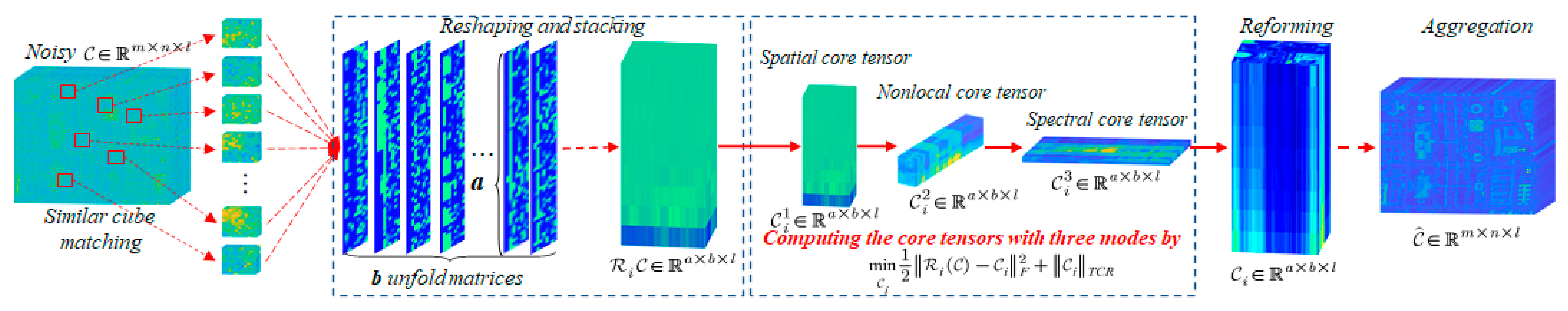
where is the tensor low-cascaded-rank minimization for the low-rank constructed tensor , and —with the linear transform operator —represents the third-order group tensor for each exemplar cube at location i. The flow of the tensor low-cascaded-rank decomposition can now be determined, as shown in Figure 1; this exploits the intrinsic correlation along spatial, nonlocal, and spectral modes of with the cascaded manner. More details about how to solve Equation (5) may be found in [9].
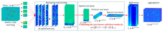
Figure 1.
Illustration for Tensor Low-Cascaded-Rank Decomposition.
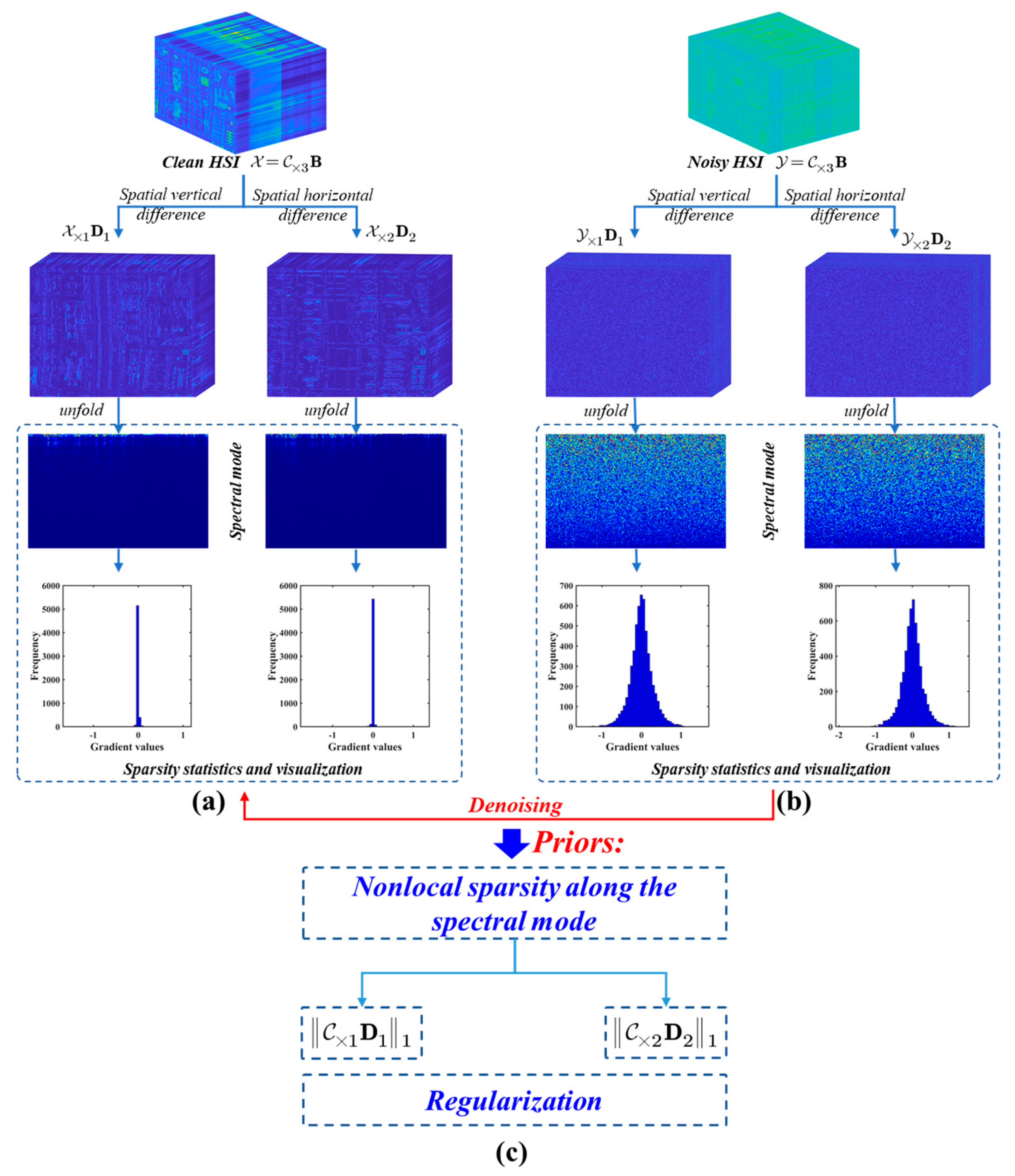
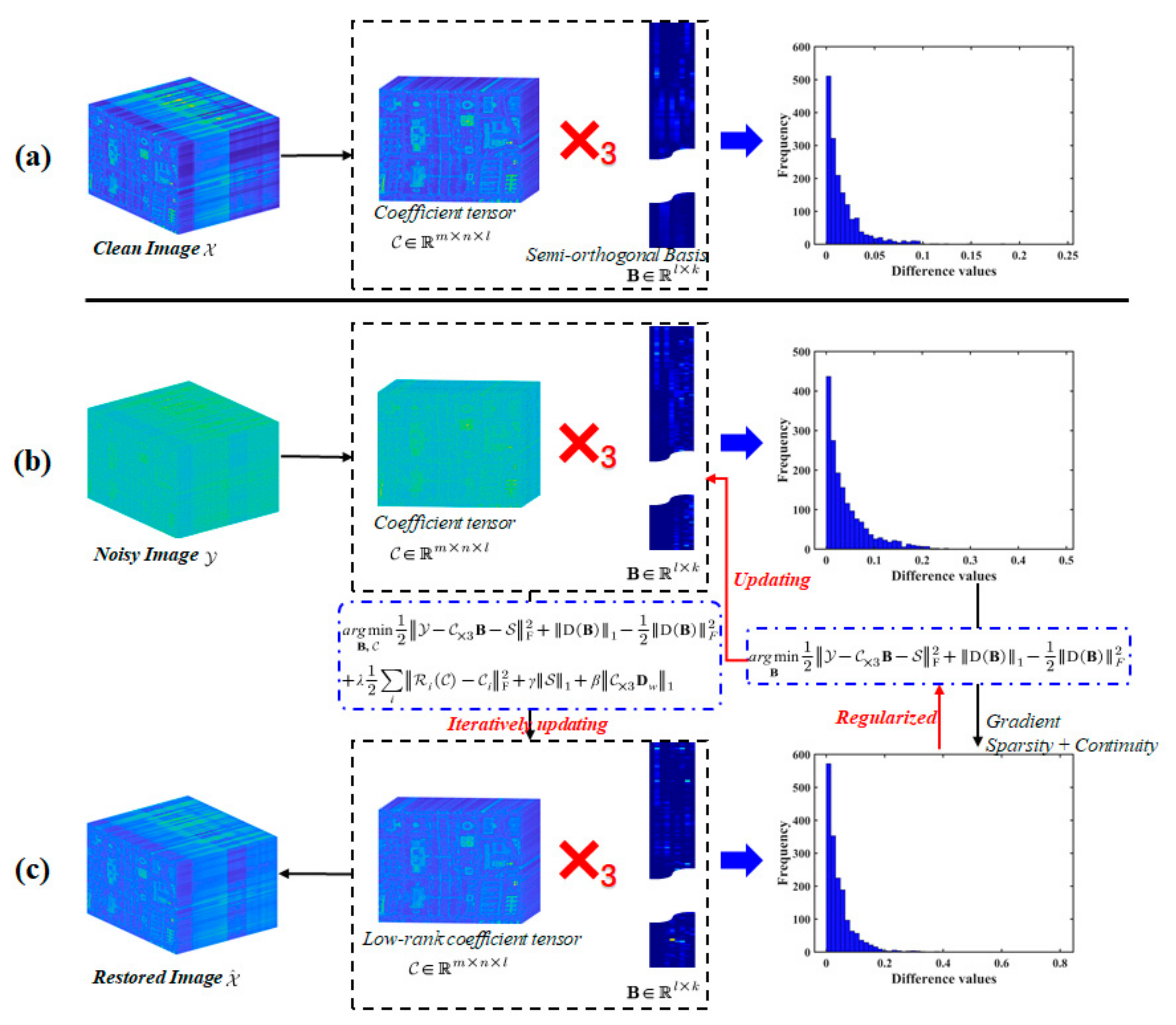
Obviously, the tensor low cascaded rank only considers the subsequent decomposition and reversion of the nonlocal cube along spatial, nonlocal, and spectral modes; the nonlocal sparsity property of for the three modes is ignored. To consider the spectral nonlocal sparsity and spectral continuity for the global HSI , we introduce a regularization for , i.e., , as shown in Figure 2. Upon analysis of Figure 2a,b and the sparsity statistic histogram, we find that (k = 1, 2) can be distinguished among the data of the clean and degraded HSIs. Following Remark 1 in [34], the necessary characters can now be obtained so that the sparsity of is consistent with that of , and more geometrical features can be acquired by the former. We therefore use the sparsity regularization term , and this leads to an improvement in the restoration of HSIs.
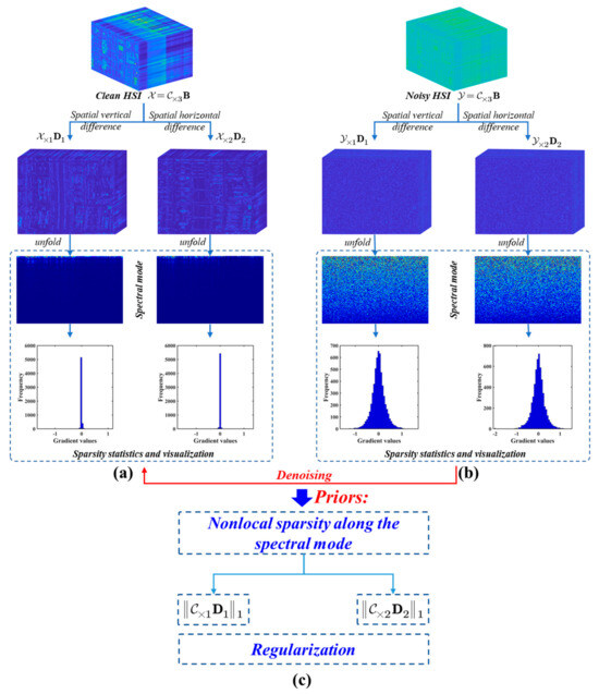
Figure 2.
Nonlocal sparsity along the spectral mode of the spatial difference images and the regularization terms based on the spatial factor . (a) Clean HSI decomposed in selected subspace; and the spatial vertical and horizontal difference of the spatial factor implemented; mode-3 unfolding matrices of the corresponding difference obtained along the spectral mode; the sparsity statistics and visualization from the unfolding matrices; (b) Noisy HSI decomposed and counted for its degraded sparsity; (c) Regularization terms on the factor used to replace the regularization terms on the clean HSI.
To promote the spectral smoothness and continuity of , a continuity constraint on B with a first-order difference is used, as represented as . As reported in [9], the basis B, which spans the high-dimensional space, is responsible for guiding the generation process of spectral data. The natural spectra of HSIs tend to be smooth and continuous, and any difference serves to establish and preserve the character of a regularization term to constrain the restored basis B, resulting in an excellent restoration. Although the difference continuity regularization term of the basis B can be established according to its physical sense, its latent sparsity is also worthy of consideration. A comparison of clean, degraded, and mixed denoising results is presented in Figure 3. From the figure, it can be seen that the difference of the basis B on the clean HSI is continuous, with more zeros than the noisy HSI. Additionally, the continuity and gradient sparsity of the HSI denoising results exhibit a distribution similar to that of the clean results, while that of the noisy HSI can be distinguished. As such, continuity and gradient sparsity can be abstracted as regularized terms based on the L1–2 norm. In summary, the double-factor tensor low-cascaded-rank minimization for the HSI denoising model can be defined as follows:
where stand for the first-order difference matrices.

Figure 3.
Illustration of the spatial continuity and sparsity for the difference of the basis B. (a–c) Clean, noisy, and restored HSIs with subspace decomposition, spatial continuity, and sparsity statistics of the difference of the basis B, respectively. Due to the difference between noisy HSI and restored or clean HSI, the necessary regularization term based on the L1–2 norm can be used, which is composed of the TCR and gradient sparsity, with to obtain the objective function for the new denoising method with an iterative update.
2.2. Efficient Alternating Optimization for Solving the Denoising Algorithm
According to ADMM optimization, the minimization problem (6) can be solved using the following formulae:
The tensors in the first formula of Equation (7) can be estimated using a two-fold approach, i.e., by considering the decomposition and reversion of the core tensors along spatial, nonlocal, and spectral modes in a cascaded manner. The processes need to be completed by cube matching and grouping, as shown in Figure 1. Further details on the use of this approach to estimate the core tensors can be found in [9]. The estimation of and involves a typically nonconvex problem which is difficult to solve directly. The efficient ADMM-based framework is therefore utilized for optimization due to its guaranteed convergence rate [52,53]. The intermediate variables , , and are now introduced for decoupling purposes, and the second formula of Equation (7) can be recast as follows:
The solution to Equation (8) with constraints is equivalent to minimizing the Lagrangian function:
where , , and are the augmented Lagrange multipliers; and , , and are the positive penalty scalar parameters. These parameters are now the subjects of a series of subproblems, as follows.
2.2.1. -Subproblem
The first subproblem is to update , whose expression is written thus:
Obviously, Equation (10) is a quadratic regularized least-square problem; this can be expressed using the following equation:
2.2.2. , , and -Subproblems Based on L1 Norm
The second subproblem is related to , , and . This can be expressed by the following equations:
The solutions to Equations (12), (13), and (14) may now be expressed as (15), (16), and (17), respectively, as follows:
2.2.3. -Subproblem
The subproblem of updating can be expressed as follows:
The solution to Equation (18) is obtained using Equation (19), as follows:
Equation (19) may now be rewritten thus:
where K(3) is the matrix format of , i.e.,
We are now presented with an obvious Sylvester matrix equation, which may be solved using the following method: first, the circulant matrix and the symmetric matrix are implemented with 1-D fast Fourier transformation and eigenvalue decomposition, respectively [9,34]. This process may be expressed as follows:
where is a 1 − D discrete Fourier transform (DFT) matrix. Having obtained a first solution of the Sylvester matrix equation, can now be calculated using the following equation:
where ; represents component-wise multiplication, and represents component-wise division.
2.2.4. -Subproblem
The subproblem of updating B may be expressed as in Equation (22), as follows:
Equation (22) expresses a quadratic optimization problem similar to the -subproblem described above; therefore, B can now be formulated, as follows:
where . Due to the circulant matrix of and the symmetric matrix of , the solution B can be obtained, thus:
where and are the fast Fourier transform operator and its inverse, respectively; is a matrix whose diagonal entries are 1 and all others are 0; is an all-ones matrix; and U and are the eigen matrix and eigenvalues matrix, respectively.
2.2.5. Updating Lagrangian Multipliers
Finally, according to the alternating optimization framework of ADMM, the update of the Lagrangian multipliers is obtained using the following equations:
The above derivations and analyses make it obvious that the optimization procedures must be conducted by means of iteration; this is summarized in Algorithm 1 for the denoising of HSIs.
| Algorithm 1 Proposed algorithm for HSI denoising |
| Input: A rearranged noisy HSI tensor . |
| Initialization: Estimate B0 with SVD, set ; regularization parameters , , and ; Subspace dimension ; Cube matching parameter a, b; Tensor cascaded rank ; Stop criterion , positive scalar , , , , , , and ; maximum iteration . |
| Tensor Low-cascaded-rank decomposition: estimate by Equation (7). |
| While not converged do |
| Sparse noise estimation: calculate by Equation (15); |
| Latent input HSI estimation: calculate by Equation (10); |
| Tensor coefficient learning: calculate by Equation (18); |
| Continuous basis learning: calculate by Equation (24); |
| Auxiliary variables estimation: calculate by Equations (16) and (17) |
| Update lagrangian multiplier by Equation (25), Equation (26), Equation (27), respectively; |
| Update penalty scalar: , |
| , ; |
| Check the convergence: or functional energy: |
| ; |
| Update iteration: . |
| End while |
| Output. |
3. Experimentation
In this section, we describe a number of simulated and real-world experiments that were conducted to assess the performance of the proposed DFTCR denoising method. In brief, we sought to compare the denoising performance of the proposed DFTCR with that of eleven state-of-the-art denoising methods. These were BM4D [13], LRMR [31], LRTDTV [37], WLRTR [32], FGLR [36], NGMeet [19], NLSSR [21], FGSLR [35], NFF [53], SDeCNN [41], and STCR [9]. It should be noted that SDeCNN is a deep learning method whose pretrained model was directly used as the best-performing model. All experiments were conducted using Windows 10 on an Intel Xeon 2.89-GHz CPU with 128 GB of memory. To obtain a fair comparison, the setting of parameters was carried out in line with the published instructions for each competing method.
3.1. Experiment Setup
Datasets: In order to verify the robustness and performance of the proposed DFTCR method, the necessary numerical experiments were carried out using the famous HYDICE Washington DC Mall dataset (WDC, https://engineering.purdue.edu/biehl/MultiSpec/hyperspectral.html, accessed on 17 December 2023) for simulation purposes. The size of the synthetic HSI was 300 × 300 × 191. There are several different types of noise in real-world HSIs, including Gaussian, impulse, deadline, and stripe noise. In real-world scenarios involving HSIs, such noises usually manifest as a mixture of several kinds. Therefore, to simulate such scenarios as well as possible, four different noise cases based on the mixed-noise settings of the compared methods were thoroughly compared. Before simulation, the gray values of each band were normalized.
Case 1 (Gaussian noise): zero-mean Gaussian noise with a variance of 0.15, 0.30, or 0.45 was added to all bands.
Case 2 (Gaussian noise + impulse noise): A mixture of zero-mean Gaussian noise and impulse noise was added to all bands. The variance of Gaussian noise was set as = 0.3, and percentages of impulse noise were randomly sampled within a range of [0, 0.2].
Case 3 (Gaussian noise + impulse noise + deadlines): A mixture of zero-mean Gaussian noise, impulse noise, and deadlines was added to all bands. The variance of Gaussian noise was set as = 0.15, and percentages of impulse noise were randomly sampled within a range of [0, 0.2]. Deadlines, affecting 10% of the columns or rows of the HSIs, were added into the 91–130 bands.
Case 4 (Gaussian noise + impulse noise + stripes): A mixture of zero-mean Gaussian noise, impulse noise, and stripes was added to all bands. The variance of Gaussian noise was set as = 0.15, and the percentages of impulse noise were randomly sampled within a range of [0, 0.2]. Stripes, affecting 10% of the columns or rows of the HSIs, were added to the 131–190 bands.
Because the ground-truth HSI was obtained from the simulated experiments, three quantitative figure indices from the comparison were employed: mean peak signal-to-noise ratio (MPSNR) over all bands; mean structure similarity (MSSIM) over all bands; and mean spectral angle mapping (MSAM) over all spectral vectors. The greater the values of MPSNR and MSSIM and the smaller the value of MSAM, the better the HSI denoising results.
The regularization parameters , , and were selected in the intervals , and , respectively. The cube matching parameters a and b, and the tensor cascaded rank were selected as , , and , respectively, following [9]. In our experiments, all parameters were set consistently, as follows: , , , , , and . The stopping condition was set as ; the penalty parameters were set as , the maxima of which were ; the multiplier scale was ; and the maximum iteration was set as 50. Finally, , where , , and represent the singular value decomposition (SVD) of , was vectorized from HSI along the spatial dimension.
3.2. Denoising Results for Simulated Noisy HSIs
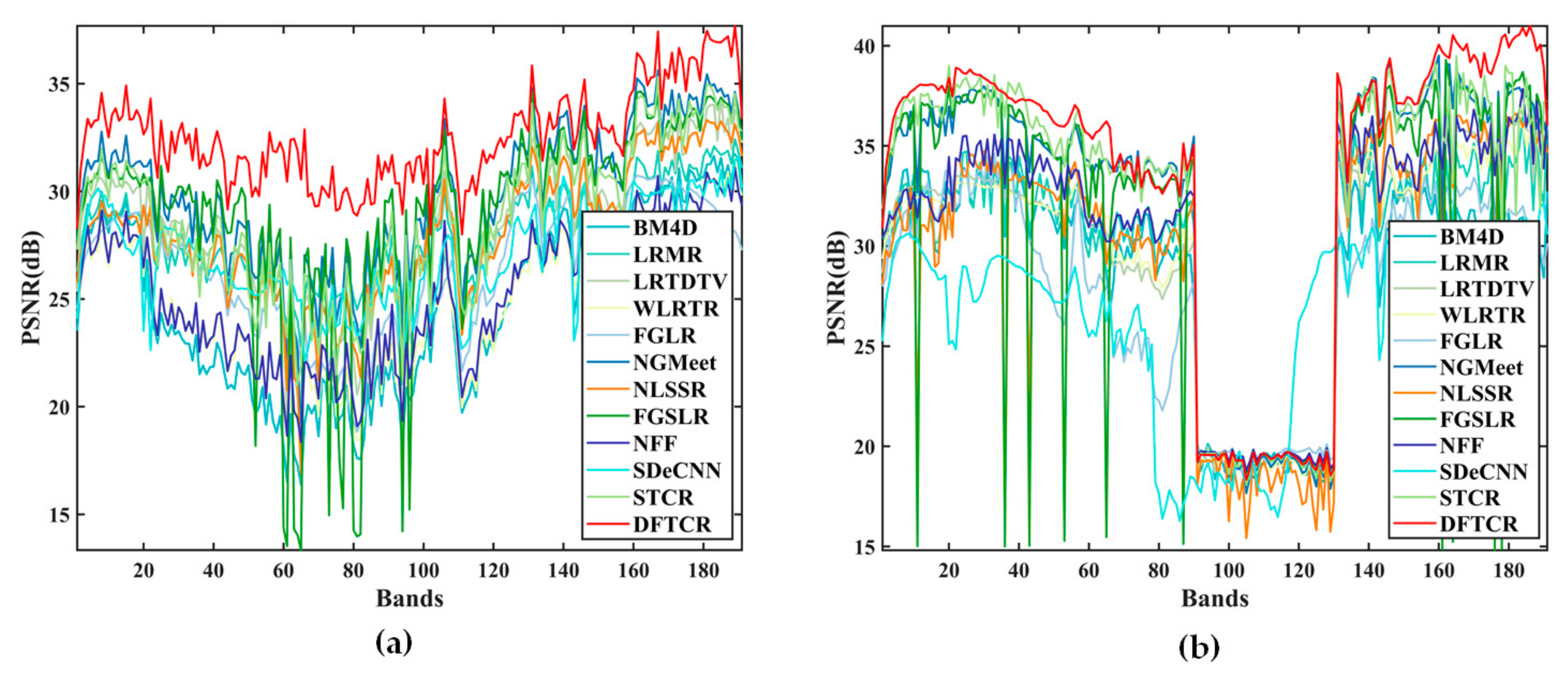
The MPSNR, MSSIM, and MSAM values produced by all the competing methods are shown in Table 1. The best results are highlighted in bold, and the second-best results are presented in italic format. It can be seen that the proposed DFTCR method achieved results that were superior to those of competitors in almost all cases. In particular, DFTCR achieved the best MPSNR values, and most of its MSSIM and MSAM results were superior to those achieved by competitors. However, the NGMeet method did achieve some MSSIM and MSAM results, which were superior to those of the proposed DFTCR method. For a comparison of performances with respect to individual bands, Figure 4 gives the PSNR values for each band obtained by all the compared methods in Cases 3 and 4. In Figure 4b, it can be seen that a group of very low PSNR values covers the band range from 91 to 130; this indicates the effect of the mixed noise, including the Gaussian noise and impulse noise. It is a challenge for all denoising methods to achieve restoration under such conditions. However, a high value was maintained by the proposed DFTCR, so that the negative effects of the mixed noise were removed. It can also be seen that the proposed DFTCR achieved the highest PSNR values of all the competing methods. This implies that the proposed method is able to achieve high-quality denoising results.

Table 1.
Three quantitative results of comparison methods under different cases for WDC datasets.
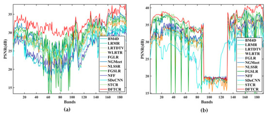
Figure 4.
PSNR values of each band of the simulated WDC dataset with Case 3 and Case 4. (a) Case 3. (b) Case 4.
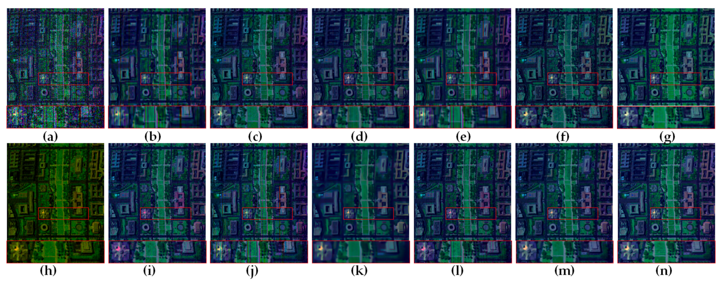
To better compare the denoising results for these restored images, Figure 5 and Figure 6 show pseudo-color images of the WDC HSIs (composed of bands 150, 89, and 46; and 180, 161, and 70) before and after denoising with different methods. It can be seen in Figure 5 that BM4D, WLRTR, NFF, and STCR produced restored HSIs, which were barely satisfactory. However, STCR achieved greater PSNR values (Table 1) than all other methods except for NGMeet, FGSLR, and DFTCR; we may therefore say that STCR effectively removes Gaussian and impulse noise. LRMR, LRTDTV, NLSSR, and FGSLR removed the most deadline noise, but some deadline residues remained in restored HSIs. In particular, NLSSR and FGSLR retained some Gaussian noise; this was not effectively removed from the zoomed-in HSIs. Moreover, a comparison with the ground-truth HSI showed that NLSSR produced digital number (DN) bias globally and FGSLR exhibited some DN bias, with pink roofs, locally. Better denoising results were achieved by FGLR and NGMeet, but some residual noise was retained in the former, and a slight DN bias was exhibited in the latter. SDeCNN achieved clear and smooth denoising results, but local details were lost. DFTCR was therefore the most suitable denoising method for deadline-contaminated HSIs. The proposed DFTCR method produced smooth and clear HSIs with abundant details without significant DN bias. In Case 3, then, the proposed DFTCR produced the best visual quality.
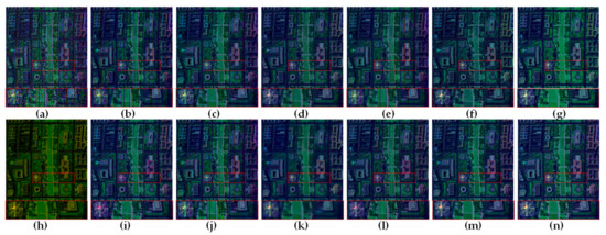
Figure 5.
Visual comparison of denoising results for the simulated WDC dataset by bands (R:150, G:89, B:46) (Case 3). (a) Noisy. (b) BM4D. (c) LRMR. (d) LRTDTV. (e) WLRTR. (f) FGLR. (g) NGMeet. (h) NLSSR. (i) FGSLR. (j) NFF. (k) SDeCNN. (l) STCR. (m) Proposed DFTCR. (n) Ground Truth.
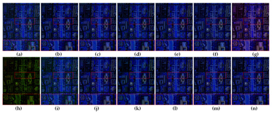
Figure 6.
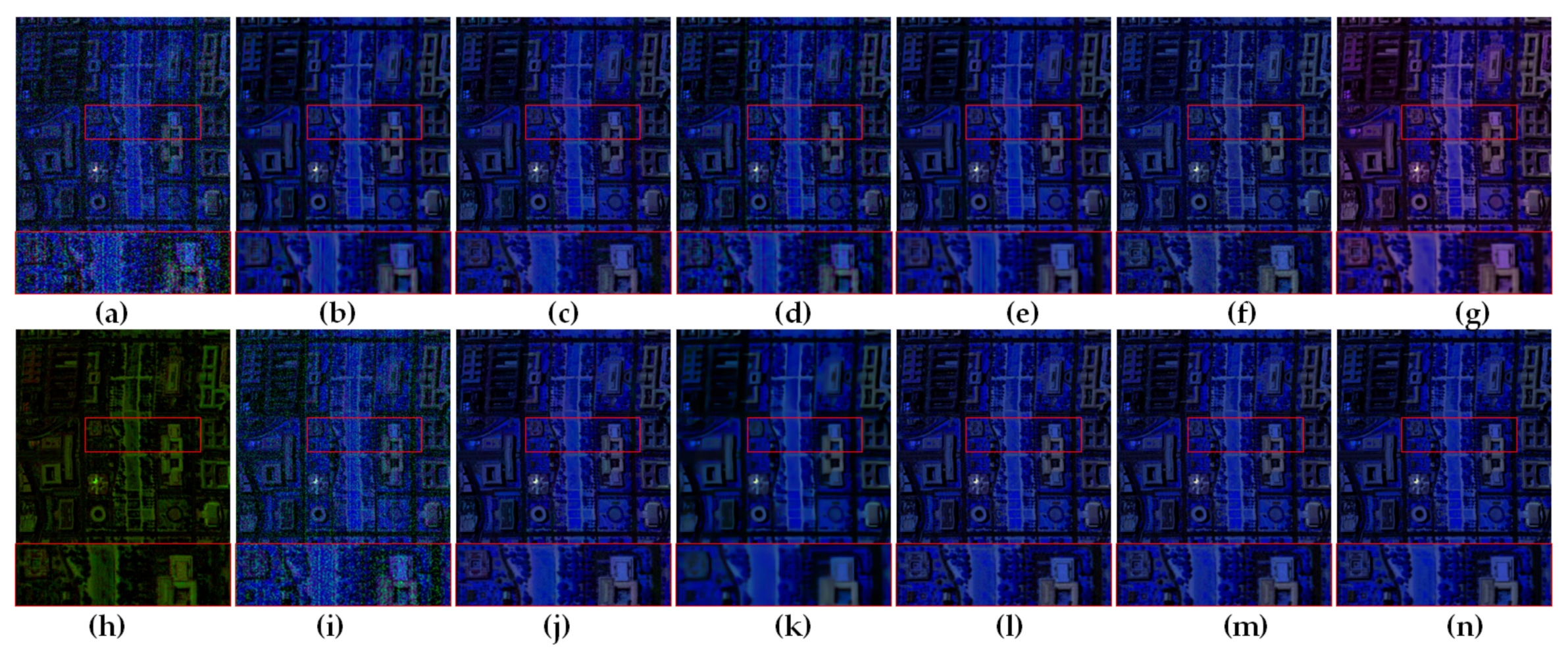
Visual comparison of denoising results for the simulated WDC dataset by bands (R:180, G:161, B:70) (Case 4). (a) Noisy. (b) BM4D. (c) LRMR. (d) LRTDTV. (e) WLRTR. (f) FGLR. (g) NGMeet. (h) NLSSR. (i) FGSLR. (j) NFF. (k) SDeCNN. (l) STCR. (m) Proposed DFTCR. (n) Ground Truth.
It is well known among scholars that inconsistencies in the mechanical motion of systems and the failure of CCD arrays lead to nonuniform responses in neighboring detectors, thereby generating stripping noise [9]. In the present study, therefore, we tested the performance of the competing denoising approaches using HSIs contaminated by stripes. The results are shown in Figure 6, in which local details are zoomed-in within red rectangles. It can be seen that FGLSR failed to effectively remove the effect of noise. BM4D, LRMR, LRTDTV, WLRTR, and NLSSR all restored clean HSIs but with a few residual stripes; among these, NLSSR also produced serious DN biases, compared with the ground-truth HSI. FGLR and NGMeet produced cleaner HSIs, but with DN biases that were minor in the case of FGLR but severe in the case of NGMeet. It can also be seen that, although SDeCNN produced a clean and smoothed HSI, the edges of the building are blurred, and its details are lost. The remaining denoising methods produced HSIs of better quality without significant visual differences and preserved abundant details without color skews. From these results, along with those presented in Table 1, it may be determined that the proposed DFTCR produced the highest MPSNR value and the second-highest MSSIM value, while NGMeet produced the highest-ranked MSSIM and NFF the highest-ranked MSAM. In summary, then, we may say that the proposed DFTCR exhibited state-of-the-art performance in HSI denoising.
3.3. Denoising Results for Real-World Noisy HSIs
The above section describes the extensive simulated experiments that were carried out to demonstrate the superiority of the proposed DFTCR. In the next section, we report our use of four real-world HSIs from two sensors, i.e., AVIRIS and AHSI. The real Indian Pines dataset with a size of 145 × 145 × 220 (obtained from https://www.ehu.eus/ccwintco/index.php/Hyperspectral_Remote_Sensing_Scenes, accessed on 17 December 2023) with serious levels of noise from the AVIRIS sensor was utilized, and the denoising results are illustrated in Figure 7 in pseudo-color format. Most of these methods exhibited good performance in removing Gaussian noise and were able to recover more details without color skew, except for NGMeet and NLSSR. NGMeet produced redder and smoother regions with some loss of detail, and NLSSR produced a similar result but with greener regions. Comparing the STCR with the proposed DFTCR, we found that both removed Gaussian noise effectively; in particular, the proposed DFTCR preserved smoother regions with details.
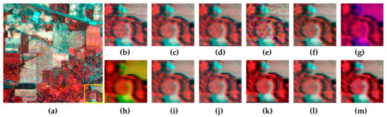
Figure 7.
Visual comparison of denoising results for the real Indian Pines dataset by bands (R:89, G:27, B:17). (a) Noisy. (b) BM4D. (c) LRMR. (d) LRTDTV. (e) WLRTR. (f) FGLR. (g) NGMeet. (h) NLSSR. (i) FGSLR. (j) NFF. (k) SDeCNN. (l) STCR. (m) Proposed DFTCR.
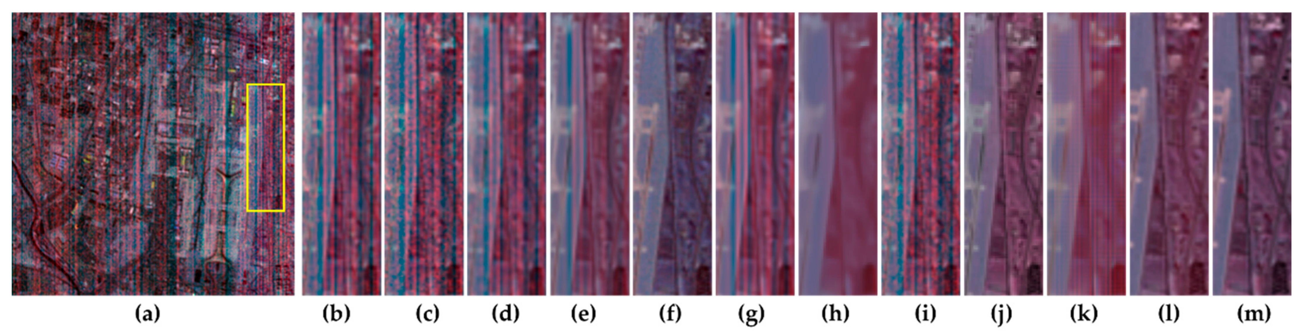
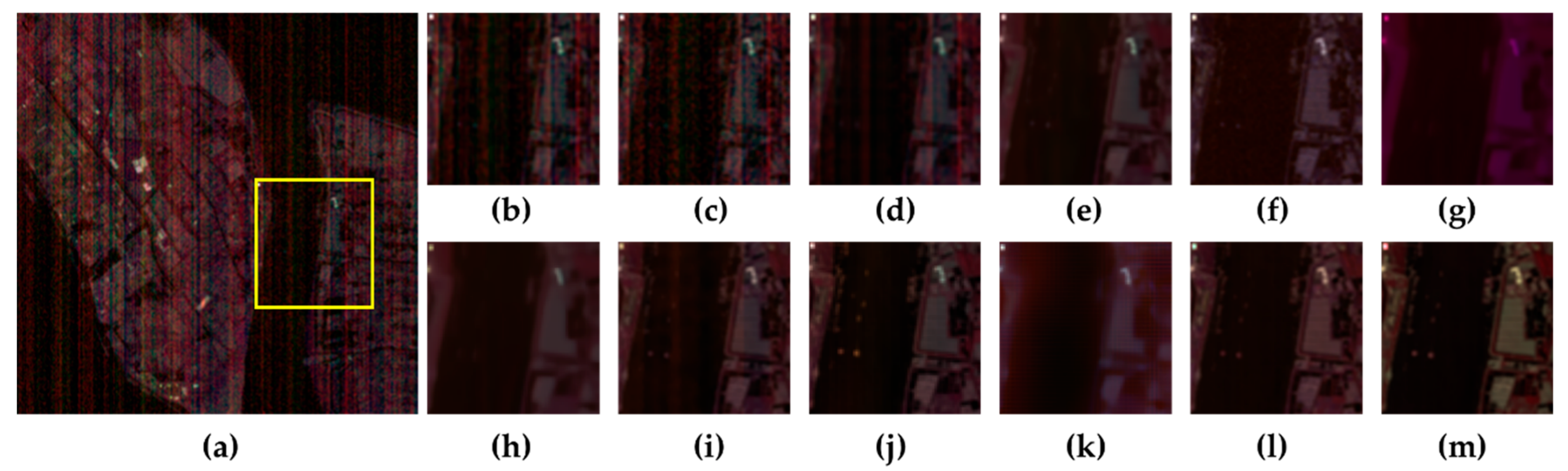
In contrast to the AVIRIS Indian Pines dataset, the Gaofen-5 (GF-5) satellite dataset (obtained from http://hipag.whu.edu.cn/resourcesdownload.html, accessed on 17 December 2023) contains dense deadlines and stripes in addition to Gaussian noise in pseudo-color noisy HSIs, as shown in Figure 8, Figure 9 and Figure 10. It can be seen that BM4D, LRMR, and LRTDTV all failed to remove these deadlines and stripes. WLRTR, NLSSR, and SDeCNN successfully removed deadlines and stripes, but details were not well preserved. NGMeet still produced a color-skew, and some details were lost. FGSLR and NFF removed all noise but still retained some spectrum offset from local color vestiges. FGLR, STCR, and the proposed DFTCR all produced clean images with rich details.
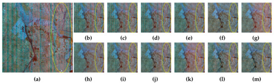
Figure 8.
Visual comparison of denoising results for the real GF−5 dataset by bands (R:155, G:102, B:46) (Baoqing). (a) Noisy. (b) BM4D. (c) LRMR. (d) LRTDTV. (e) WLRTR. (f) FGLR. (g) NGMeet. (h) NLSSR. (i) FGSLR. (j)NFF. (k) SDeCNN. (l) STCR. (m) Proposed DFTCR.
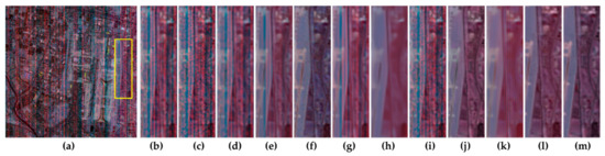
Figure 9.
Visual comparison of denoising results for the real GF−5 dataset by bands (R:155, G:102, B:46) (Capital Airport). (a) Noisy. (b) BM4D. (c) LRMR. (d) LRTDTV. (e) WLRTR. (f) FGLR. (g) NGMeet. (h) NLSSR. (i) FGSLR. (j) NFF. (k) SDeCNN. (l) STCR. (m) Proposed DFTCR.
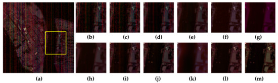
Figure 10.
Visual comparison of denoising results for the real GF−5 dataset by bands (R:155, G:102, B:46) (Shanghai). (a) Noisy. (b) BM4D. (c) LRMR. (d) LRTDTV. (e) WLRTR. (f) FGLR. (g) NGMeet. (h) NLSSR. (i) FGSLR. (j) NFF. (k) SDeCNN. (l) STCR. (m) Proposed DFTCR.
From the detail in Figure 8, it can be seen that STCR still retained a small degree of yellow-ellipse color distortion. The restored result of FGLR revealed consistency with the global color but with the color-skew trending to cyan. The proposed DFTCR produced no visible color distortion. In Figure 9, the zoomed-in regions of interest (ROIs) within yellow rectangles show sharpness in airport pavements and highways. It can also be seen that the proposed DFTCR produced a superior denoising result with sharp contrasts and edges compared with STCR, NFF, and FGLR. Furthermore, in the ROIs shown in the zoomed-in yellow rectangles of Figure 10, the stripes were removed from the river by WLRTR, FGLR, NGMeet, NLSSR, NFF, SDeCNN, STCR, and DFTCR, while the ships and other objects on the river (i.e., high-frequency information) were considered as sparse noise to be removed by WLRTR, FGLR, NGMeet, NLSSR, and SDeCNN. In addition, NFF, STCR, and DFTCR recognized high-frequency noise and information more robustly, and DFTCR retained more sharpness of classification types visually. To summarize, we may say that DFTCR eliminated the distortion from stripes and deadlines and preserved more original spectral information at the same time, with the help of the nonlocal sparsity property with TCR prior and double actors—the basis factor B and spatial factor . This demonstrates that the proposed DFTCR is suitable for real-world HSI denoising applications.
4. Discussion
4.1. Analysis of Computation Complexity
We analyzed the computational complexity of the developed ADMM-based algorithm using the noisy HSI . In Algorithm 1, the calculation complexity at each iteration is dependent on the updating of . The complexity of the TCR decomposition before iteration is . is then updated via Equation (24), containing SVD, 1-D FFT and matrix multiplications, leading to cost. Next, updating via Equation (21) requires cost. The necessary updating costs of from Equations (15), (16), and (17) are , , and , respectively. The updating costs of from Equations (15), (16), and (17) are , , and , respectively. Finally, the sum of the computational cost at each outer iteration is .
4.2. Ablation Analysis
Comparing the objective functions of STCR and DFTCR, we find that the main distinction lies in the spatial factor . However, if we remove the regularization term from Equation (6), the DFTCR denoising method is as degraded as the STCR method. The restored results using the simulated WDC dataset for these same cases are displayed in Table 2. It can be seen that the restoration quality of HSIs increases with the participation of the regularization term. This implies that the regularization term is effective in improving restoration quality.
Table 2.
Ablation analysis without the main regularization term .
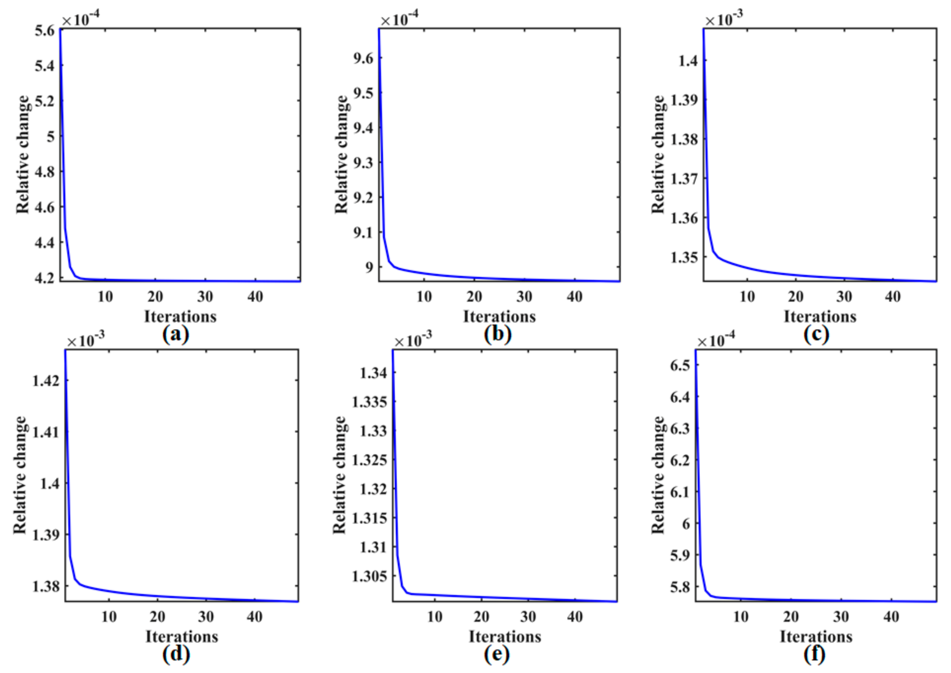
4.3. Convergence Analysis
Figure 11 represents the relative change values of the proposed DFTCR method using the simulated WDC dataset with designed cases. Six groups for four cases were employed to validate the convergence of DFTCR. From the figure, it can be seen that the curve of the relative change value monotonically converges to certain values as the number of iterations increases. In other words, the curve finally becomes flat and stable. This indicates that numerical convergence is guaranteed by the proposed DFTCR method.
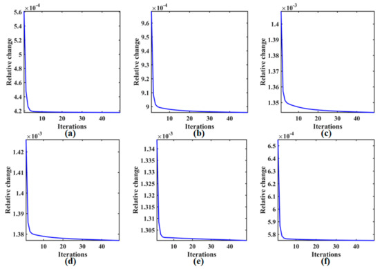
Figure 11.
Relative change values versus the iteration number of the proposed DFTCR solver in the simulated WDC dataset with designed cases. (a) Case 1 ( = 0.15). (b) Case 1 ( = 0.3). (c) Case 1 ( = 0.45). (d) Case 2. (e) Case 3. (f) Case 4.
4.4. Running Time
As described in Section 4.1 above, the proposed DFTCR method is characterized by a medium level of computation complexity. To test the running times of DFTCR, we used the real-world GF-5 Shanghai and Indian Pines datasets to compute the running times of all compared methods; these are presented in Table 3. Although all running times indicate a medium level of efficiency, the restoration qualities of DFTCR are the best among the competing methods. Overall, we may say that the proposed DFTCR strikes an effective balance between restoration quality and efficiency in the denoising of HSIs.
Table 3.
Running times (in seconds) of different methods for the real-world and simulated dataset.
5. Conclusions and Outlooks
In this paper, we describe a new HSI denoising method based on double-factor tensor cascaded-rank minimization. This method can effectively remove Gaussian noise, deadlines, and stripe noise, both individually and in combination. Due to the loss of information in the nonlocal sparsity property of the spatial factor , a necessary and robust regularization term was employed in the STCR framework. The spatial factor can be regularized to characterize the representation of geometrical features. In addition, to preserve the edges and sharpness of restored HSIs, a tensor cascaded-rank minimization prior, suggested as a nonlocal self-similarity, was fully exploited. Another factor, difference continuity and nonlocal gradient sparsity regularization, was also utilized in the proposed DFTCR to learn the basis B in its subspace and thus more closely approximate the HSIs endmembers [8,9]. The ADMM strategy can be used to derive these formulae, which form the basis of the iterative algorithm and flow. A low-dimensional subspace projection was applied to decrease the high-dimensional HSI tensor, which reduced computational complexity. Many other SOTA denoising methods for HSIs were tested as competitors to verify the performance of the proposed DFTCR. Extensive simulated and real-world experiments demonstrated the superiority and effectiveness of the proposed DFTCR in typical HSI denoising applications.
In future works, we will extend the proposed DFTCR methods to restore more types of degraded HSIs, using such techniques as deblurring, inpainting, and super-resolution reconstruction. We will also consider how to improve the computational efficiency of DFTCR and apply the method to multitemporal HSIs and satellite videos, in addition to stationary satellite images.
Author Contributions
Conceptualization, methodology, validation, investigation, writing, supervision, revision, funding acquisition, J.H.; conceptualization, methodology, original draft preparation, C.P.; supervision, review, revision, funding acquisition, project administration, H.D.; conceptualization, review, Z.Z. All authors have read and agreed to the published version of the manuscript.
Funding
This research was funded by the Technology Innovation Center for Integrated Applications in Remote Sensing and Navigation, Ministry of Natural Resources, P.R. China, under Grant TICIARSN-2023-02, the Startup Foundation for Introducing Talent of NUIST under Grant 2022R118, the Natural Science Research of the Jiangsu Higher Education Institutions of China under Grant 23KJB420003, and the Major Project of High Resolution Earth Observation System under Grant 30-Y60B01-9003-22/23.
Data Availability Statement
Data are contained within the article from these provided websites.
Acknowledgments
We thank anonymous reviewers for their comments on improving this manuscript.
Conflicts of Interest
The authors declare no conflicts of interest.
References
- Driss, H.; John, R.M.; Elizabeth, P.; Pablo, J.Z.-T.; Ian, B.S. Hyperspectral vegetation indices and novel algorithms for predicting green LAI of crop canopies: Modeling and validation in the context of precision agriculture. Remote Sens. Environ. 2004, 90, 337–352. [Google Scholar] [CrossRef]
- Bioucas-Dias, J.M.; Plaza, A.; Dobigeon, N.; Parente, M.; Du, Q.; Gader, P.; Chanussot, J. Hyperspectral Unmixing Overview: Geometrical, Statistical, and Sparse Regression-Based Approaches. IEEE J. Sel. Top. Appl. Earth Obs. Remote Sens. 2012, 5, 354–379. [Google Scholar] [CrossRef]
- Bioucas-Dias, J.M.; Plaza, A.; Camps-Valls, G.; Scheunders, P.; Nasrabadi, N.; Chanussot, J. Hyperspectral Remote Sensing Data Analysis and Future Challenges. IEEE Geosci. Remote Sens. Mag. 2013, 1, 6–36. [Google Scholar] [CrossRef]
- Shen, F.; Zhao, H.; Zhu, Q.; Sun, X.; Liu, Y. Chinese Hyperspectral Satellite Missions and Preliminary Applications of Aquatic Environment. In Proceedings of the 2021 IEEE International Geoscience and Remote Sensing Symposium IGARSS, Brussels, Belgium, 11–16 July 2021; pp. 1233–1236. [Google Scholar]
- Zürn, J.; Burgard, W.; Valada, A. Self-Supervised Visual Terrain Classification from Unsupervised Acoustic Feature Learning. IEEE Trans. Robot. 2021, 37, 466–481. [Google Scholar] [CrossRef]
- Antonio, P.; Jon, A.B.; Joseph, W.B.; Jason, B.; Lorenzo, B.; Gustavo, C.-V.; Jocelyn, C.; Mathieu, F.; Paolo, G.; Anthony, G.; et al. Recent advances in techniques for hyperspectral image processing. Remote Sens. Environ. 2009, 113, S110–S122. [Google Scholar] [CrossRef]
- Willett, R.M.; Duarte, M.F.; Davenport, M.A.; Baraniuk, R.G. Sparsity and Structure in Hyperspectral Imaging: Sensing, Reconstruction, and Target Detection. IEEE Signal Process. Mag. 2014, 31, 116–126. [Google Scholar] [CrossRef]
- Sun, L.; Cao, Q.; Chen, Y.; Zheng, Y.; Wu, Z. Mixed Noise Removal for Hyperspectral Images Based on Global Tensor Low-Rankness and Nonlocal SVD-Aided Group Sparsity. IEEE Trans. Geosci. Remote Sens. 2023, 61, 1–17. [Google Scholar] [CrossRef]
- Sun, L.; He, C.; Zheng, Y.; Wu, Z.; Jeon, B. Tensor Cascaded-Rank Minimization in Subspace: A Unified Regime for Hyperspectral Image Low-Level Vision. IEEE Trans. Image Process. 2023, 32, 100–115. [Google Scholar] [CrossRef]
- Zhang, H.; Chen, H.; Yang, G.; Zhang, L. LR-Net: Low-Rank Spatial-Spectral Network for Hyperspectral Image Denoising. IEEE Trans. Image Process. 2021, 30, 8743–8758. [Google Scholar] [CrossRef]
- Elad, M. On the origin of the bilateral filter and ways to improve it. IEEE Trans. Image Process. 2002, 11, 1141–1151. [Google Scholar] [CrossRef]
- Dabov, K.; Foi, A.; Katkovnik, V.; Egiazarian, K. Image Denoising by Sparse 3-D Transform-Domain Collaborative Filtering. IEEE Trans. Image Process. 2007, 16, 2080–2095. [Google Scholar] [CrossRef] [PubMed]
- Maggioni, M.; Katkovnik, V.; Egiazarian, K.; Foi, A. Nonlocal Transform-Domain Filter for Volumetric Data Denoising and Reconstruction. IEEE Trans. Image Process. 2013, 22, 119–133. [Google Scholar] [CrossRef] [PubMed]
- Maggioni, M.; Boracchi, G.; Foi, A.; Egiazarian, K. Video Denoising, Deblocking, and Enhancement Through Separable 4-D Nonlocal Spatiotemporal Transforms. IEEE Trans. Image Process. 2012, 21, 3952–3966. [Google Scholar] [CrossRef] [PubMed]
- Chen, G.; Tien, D.B.; Kha, G.Q.; Qian, S.-E. Denoising Hyperspectral Imagery Using Principal Component Analysis and Block-Matching 4D Filtering. Can. J. Remote Sens. 2014, 40, 60–66. [Google Scholar] [CrossRef]
- Buades, A.; Coll, B.; Morel, J.-M. A non-local algorithm for image denoising. In Proceedings of the 2005 IEEE Computer Society Conference on Computer Vision and Pattern Recognition (CVPR’05), San Diego, CA, USA, 20–25 June 2005; Volume 2, pp. 60–65. [Google Scholar]
- Dong, W.; Huang, T.; Shi, G.; Ma, Y.; Li, X. Robust Tensor Approximation with Laplacian Scale Mixture Modeling for Multiframe Image and Video Denoising. IEEE J. Sel. Top. Signal Process. 2018, 12, 1435–1448. [Google Scholar] [CrossRef]
- Ge, Q.; Jing, X.-Y.; Wu, F.; Wei, Z.-H.; Xiao, L.; Shao, W.-Z.; Yue, D.; Li, H.-B. Structure-Based Low-Rank Model with Graph Nuclear Norm Regularization for Noise Removal. IEEE Trans. Image Process. 2017, 26, 3098–3112. [Google Scholar] [CrossRef] [PubMed]
- He, W.; Yao, Q.; Li, C.; Yokoya, N.; Zhao, Q.; Zhang, H.; Zhang, L. Non-Local Meets Global: An Iterative Paradigm for Hyperspectral Image Restoration. IEEE Trans. Pattern Anal. Mach. Intell. 2022, 44, 2089–2107. [Google Scholar] [CrossRef] [PubMed]
- Zhuang, L.; Fu, X.; Ng, M.K.; Bioucas-Dias, J.M. Hyperspectral Image Denoising Based on Global and Nonlocal Low-Rank Factorizations. IEEE Trans. Geosci. Remote Sens. 2021, 59, 10438–10454. [Google Scholar] [CrossRef]
- Zha, Z.; Wen, B.; Yuan, X.; Zhang, J.; Zhou, J.; Lu, Y.; Zhu, C. Nonlocal Structured Sparsity Regularization Modeling for Hyperspectral Image Denoising. IEEE Trans. Geosci. Remote Sens. 2023, 61, 1–16. [Google Scholar] [CrossRef]
- Aggarwal, H.K.; Majumdar, A. Hyperspectral Image Denoising Using Spatio-Spectral Total Variation. IEEE Geosci. Remote Sens. Lett. 2016, 13, 442–446. [Google Scholar] [CrossRef]
- Yuan, Q.; Zhang, L.; Shen, H. Hyperspectral Image Denoising Employing a Spectral–Spatial Adaptive Total Variation Model. IEEE Trans. Geosci. Remote Sens. 2012, 50, 3660–3677. [Google Scholar] [CrossRef]
- Qian, Y.; Ye, M. Hyperspectral Imagery Restoration Using Nonlocal Spectral-Spatial Structured Sparse Representation With Noise Estimation. IEEE J. Sel. Top. Appl. Earth Obs. Remote Sens. 2013, 6, 499–515. [Google Scholar] [CrossRef]
- He, W.; Zhang, H.; Zhang, L.; Shen, H. Total-Variation-Regularized Low-Rank Matrix Factorization for Hyperspectral Image Restoration. IEEE Trans. Geosci. Remote Sens. 2016, 54, 178–188. [Google Scholar] [CrossRef]
- Lu, T.; Li, S.; Fang, L.; Ma, Y.; Benediktsson, J.A. Spectral–Spatial Adaptive Sparse Representation for Hyperspectral Image Denoising. IEEE Trans. Geosci. Remote Sens. 2016, 54, 373–385. [Google Scholar] [CrossRef]
- Rasti, B.; Sveinsson, J.R.; Ulfarsson, M.O.; Benediktsson, J.A. Hyperspectral Image Denoising Using First Order Spectral Roughness Penalty in Wavelet Domain. IEEE J. Sel. Top. Appl. Earth Obs. Remote Sens. 2014, 7, 2458–2467. [Google Scholar] [CrossRef]
- Zhao, B.; Ulfarsson, M.O.; Sveinsson, J.R.; Chanussot, J. Hyperspectral Image Denoising Using Spectral-Spatial Transform-Based Sparse and Low-Rank Representations. IEEE Trans. Geosci. Remote Sens. 2022, 60, 1–25. [Google Scholar] [CrossRef]
- Zhuang, L.; Bioucas-Dias, J.M. Fast Hyperspectral Image Denoising and Inpainting Based on Low-Rank and Sparse Representations. IEEE J. Sel. Top. Appl. Earth Obs. Remote Sens. 2018, 11, 730–742. [Google Scholar] [CrossRef]
- Zhang, H.; He, W.; Zhang, L.; Shen, H.; Yuan, Q. Hyperspectral Image Restoration Using Low-Rank Matrix Recovery. IEEE Trans. Geosci. Remote Sens. 2014, 52, 4729–4743. [Google Scholar] [CrossRef]
- He, W.; Zhang, H.; Shen, H.; Zhang, L. Hyperspectral Image Denoising Using Local Low-Rank Matrix Recovery and Global Spatial–Spectral Total Variation. IEEE J. Sel. Top. Appl. Earth Obs. Remote Sens. 2018, 11, 713–729. [Google Scholar] [CrossRef]
- Chang, Y.; Yan, L.; Zhao, X.-L.; Fang, H.; Zhang, Z.; Zhong, S. Weighted Low-Rank Tensor Recovery for Hyperspectral Image Restoration. IEEE Trans. Cybern. 2020, 50, 4558–4572. [Google Scholar] [CrossRef]
- Chen, Y.; Guo, Y.; Wang, Y.; Wang, D.; Peng, C.; He, G. Denoising of Hyperspectral Images Using Nonconvex Low Rank Matrix Approximation. IEEE Trans. Geosci. Remote Sens. 2017, 55, 5366–5380. [Google Scholar] [CrossRef]
- Zheng, Y.-B.; Huang, T.-Z.; Zhao, X.-L.; Chen, Y.; He, W. Double-Factor-Regularized Low-Rank Tensor Factorization for Mixed Noise Removal in Hyperspectral Image. IEEE Trans. Geosci. Remote Sens. 2020, 58, 8450–8464. [Google Scholar] [CrossRef]
- Chen, Y.; Huang, T.-Z.; He, W.; Zhao, X.-L.; Zhang, H.; Zeng, J. Hyperspectral Image Denoising Using Factor Group Sparsity-Regularized Nonconvex Low-Rank Approximation. IEEE Trans. Geosci. Remote Sens. 2022, 60, 1–16. [Google Scholar] [CrossRef]
- Su, X.; Zhang, Z.; Yang, F. Fast Hyperspectral Image Denoising and Destriping Method Based on Graph Laplacian Regularization. IEEE Trans. Geosci. Remote Sens. 2023, 61, 1–14. [Google Scholar] [CrossRef]
- Chen, Y.; He, W.; Yokoya, N.; Huang, T.-Z. Hyperspectral Image Restoration Using Weighted Group Sparsity-Regularized Low-Rank Tensor Decomposition. IEEE Trans. Cybern. 2020, 50, 3556–3570. [Google Scholar] [CrossRef] [PubMed]
- Zeng, H.; Xie, X.; Cui, H.; Yin, H.; Ning, J. Hyperspectral Image Restoration via Global L1-2 Spatial–Spectral Total Variation Regularized Local Low-Rank Tensor Recovery. IEEE Trans. Geosci. Remote Sens. 2021, 59, 3309–3325. [Google Scholar] [CrossRef]
- Yuan, Q.; Zhang, Q.; Li, J.; Shen, H.; Zhang, L. Hyperspectral Image Denoising Employing a Spatial–Spectral Deep Residual Convolutional Neural Network. IEEE Trans. Geosci. Remote Sens. 2019, 57, 1205–1218. [Google Scholar] [CrossRef]
- Zhang, Q.; Yuan, Q.; Li, J.; Sun, F.; Zhang, L. Deep spatio-spectral Bayesian posterior for hyperspectral image non-i.i.d. noise removal. ISPRS J. Photogramm. Remote Sens. 2020, 164, 125–137. [Google Scholar] [CrossRef]
- Maffei, A.; Haut, J.M.; Paoletti, M.E.; Plaza, J.; Bruzzone, L.; Plaza, A. A Single Model CNN for Hyperspectral Image Denoising. IEEE Trans. Geosci. Remote Sens. 2020, 58, 2516–2529. [Google Scholar] [CrossRef]
- Murugesan, R.; Nachimuthu, N.; Prakash, G. Attention based deep convolutional U-Net with CSA optimization for hyperspectral image denoising. Infrared Phys. Technol. 2023, 129, 104531. [Google Scholar] [CrossRef]
- Chang, Y.; Yan, L.; Fang, H.; Zhong, S.; Liao, W. HSI-DeNet: Hyperspectral Image Restoration via Convolutional Neural Network. IEEE Trans. Geosci. Remote Sens. 2019, 57, 667–682. [Google Scholar] [CrossRef]
- Tucker, L.R. Some mathematical notes on three-mode factor analysis. Psychometrika 1966, 31, 279–311. [Google Scholar] [CrossRef] [PubMed]
- Carroll, J.D.; Chang, J.-J. Analysis of individual differences in multidimensional scaling via an n-way generalization of “Eckart-Young” decomposition. Psychometrika 1970, 35, 283–319. [Google Scholar] [CrossRef]
- Kilmer, M.E.; Braman, K.; Hao, N.; Hoover, R.C. Third-Order Tensors as Operators on Matrices: A Theoretical and Computational Framework with Applications in Imaging. SIAM J. Matrix Anal. Appl. 2013, 34, 148–172. [Google Scholar] [CrossRef]
- Zhang, Z.; Ely, G.; Aeron, S.; Hao, N.; Kilmer, M. Novel Methods for Multilinear Data Completion and De-noising Based on Tensor-SVD. In Proceedings of the 2014 IEEE Conference on Computer Vision and Pattern Recognition, Columbus, OH, USA, 23–28 June 2014; pp. 3842–3849. [Google Scholar]
- Oseledets, I.V. Tensor-Train Decomposition. SIAM J. Sci. Comput. 2011, 33, 2295–2317. [Google Scholar] [CrossRef]
- Zhao, Q.; Zhou, G.; Xie, S.; Zhang, L.; Cichocki, A. Tensor Ring Decomposition. arXiv 2016, arXiv:1606.05535. [Google Scholar] [CrossRef]
- Wang, M.; Hong, D.; Han, Z.; Li, J.; Yao, J.; Gao, L.; Zhang, B.; Chanussot, J. Tensor Decompositions for Hyperspectral Data Processing in Remote Sensing: A comprehensive review. IEEE Geosci. Remote Sens. Mag. 2023, 11, 26–72. [Google Scholar] [CrossRef]
- Boyd, S.; Parikh, N.; Chu, E.; Peleato, B.; Eckstein, J. Distributed Optimization and Statistical Learning via the Alternating Direction Method of Multipliers. Found. Trends Mach. Learn. 2011, 3, 1–122. [Google Scholar] [CrossRef]
- Lu, C.; Feng, J.; Yan, S.; Lin, Z. A Unified Alternating Direction Method of Multipliers by Majorization Minimization. IEEE Trans. Pattern Anal. Mach. Intell. 2018, 40, 527–541. [Google Scholar] [CrossRef]
- Liu, T.; Hu, D.; Wang, Z.; Gou, J.; Chen, W. Hyperspectral Image Denoising Using Nonconvex Fraction Function. IEEE Geosci. Remote Sens. Lett. 2023, 20, 1–5. [Google Scholar] [CrossRef]


Disclaimer/Publisher’s Note: The statements, opinions and data contained in all publications are solely those of the individual author(s) and contributor(s) and not of MDPI and/or the editor(s). MDPI and/or the editor(s) disclaim responsibility for any injury to people or property resulting from any ideas, methods, instructions or products referred to in the content. |
© 2023 by the authors. Licensee MDPI, Basel, Switzerland. This article is an open access article distributed under the terms and conditions of the Creative Commons Attribution (CC BY) license (https://creativecommons.org/licenses/by/4.0/).