Abstract
A high-frequency surface wave radar (HFSWR) is the only sensor that provides inexpensive surveillance for up to 200 nautical miles (NM) of the exclusive economic zone in the 3–5 MHz band. However, because of its long wavelength, its angular resolution is low. Multiple-input multiple-output (MIMO) technology is an attractive method to improve angular resolution. This paper proposes MIMO waveforms and their processing that can be used in HFSWR systems. This dual modulation method applies linear frequency modulation to each pulse and orthogonal polyphase codes for a few consecutive pulses to enable MIMO processing. The proposed method can effectively remove the correlation of mutual interference and exhibits excellent performance in removing multiple-time-around echoes.
1. Introduction
The high-frequency surface wave radar (HFSWR) operating in the 3–30 MHz frequency band has been recognized as an important maritime surveillance sensor for sea state monitoring and vessel detection [1,2]. Moreover, it is the only sensor that provides inexpensive over-the-horizon surveillance for up to 200 nautical miles of the exclusive economic zone using the 3–5 MHz band [3,4].
However, the HF band is used by many users for various applications. The available bandwidth is thus narrow, and the operating frequency is required to be selected in real time. The available instantaneous bandwidth is typically less than 40 kHz, resulting in a coarse-range resolution of greater than 3.75 km. In addition, because the wavelength is extremely large, even if a long antenna is used, the cross-range resolution from the angular resolution is very low, especially at long distances. So, the HFSWR resolves targets based on velocity. The velocity resolution, or Doppler resolution, can be enhanced with a long integration time, which is possible due to the large resolution cell and low Doppler frequency of the target. The low Doppler frequency is both due to the slow speed of a vessel compared with that of an aircraft and to the low operating frequency of the HF band. The target Doppler of the HFSWR system is less than a few Hertz.
Improving angular resolution is challenging, and studies have continued to enhance it. Subspace-based algorithms, such as multiple signal classification (MUSIC) and estimation of signal parameters via rational invariance techniques (ESPRIT), are popular estimators to improve angle estimation [5,6]. The matrix pencil method, also known as the generalized pencil of functions, is another well-liked estimator that processes the sampled data directly without a covariance matrix [7,8]. Extensions for simultaneous estimation of azimuth and elevation exist [9]. Recently, complicated sparse array geometries have been studied and combined with the electromagnetic vector sensor (EVS) to obtain two-dimensional (2D) direction estimation. EVSs are capable of polarization status and 2D direction estimation and are being combined with multiple-input multiple-output (MIMO) radar to reduce the intensive computation for super-resolution [10,11,12].
MIMO schemes by themselves are compelling techniques for enhancing angular resolution [13,14,15,16,17]. In HFSWR systems, which utilize large antennas with vertical polarization to enable efficient surface wave propagation, MIMO approaches have been presented in two ways. One method involves the deployment of widely separated transmitters and receivers [18], while the other method involves using co-located transmitters and linear receiver arrays [19]. The widely separated method primarily uses a beam-space multiple transmission that radiates different waveforms in different directions. In contrast, the co-located type uses different waveforms for the transmit arrays and synthesizes them at the receiver array. If appropriately placed, the co-located transmit and receive arrays can create a large virtual aperture with a small number of arrays. The key areas of MIMO radar are transmit and receive antennae placement, beamforming, and waveform design. The geometric arrangement of the transmit and receive antennas constitutes the basic setup of the MIMO scheme. Flexible beamforming has been acknowledged to have a clear advantage, even in the debates over MIMO methods [20]. Finally, a waveform design is required in a MIMO scheme to separate transmit signals at the radar receiver, specifically waveforms with orthogonal characteristics. Modulation methods for achieving orthogonality include time division multiplexing, frequency domain multiplexing, and code-domain multiplexing.
In a pulse Doppler radar, modulation can be performed within or between pulses [21]. Linear frequency modulation (LFM) or code modulation, such as Barker codes, has conventionally been used for intra-pulse modulation in radar systems. Using this intra-pulse modulation for MIMO multiplexing, the transmit waveforms should be orthogonal for all time delays because the delay at the receiver is specified by the target position, which is unknown before detection [22]. Because this is not possible, transmit waveforms are designed to minimize the sum or peak of the cross-correlation function over time delays while minimizing the sidelobe level of the autocorrelation to improve detection performance. Reference [23] proposed a design method for polyphase codes, including cyclic algorithm–new (CAN) algorithms, stopband CAN, and periodic CAN. In addition, generalized optimization methods, such as genetic or simulated annealing (SA) techniques, have been provided for flexible objective functions and parameter sets [24]. The proposed method was applied to design both the polyphase code waveform and a discrete frequency coding waveform (DFCW). A modified genetic algorithm was proposed to extend DFCW to DFCW−LFM, changing the frequency around the selected frequency [25].
On the other hand, multiplexing can be performed by pulse-to-pulse modulation. DFCW−LFM changing the center frequency of each LFM pulse was proposed for the widely separated MIMO HFSWR [26]. Code multiplexing can also be applied in this way using the same design method as intra-pulse codes. However, when performing this pulse-to-pulse modulation, it is noticed that the orthogonality is affected by the Doppler shift rather than the time delay. Some studies on Doppler-insensitive codes were also proposed [27,28]. In addition to the polyphase codes, complete complementary codes with LFM pulses were proposed for MIMO HFSWR [29]. Further, more diversities combining intra-pulse and inter-pulse modulations were proposed, including a method to change both the discrete frequency and chirp rate [30]. More diversity can improve performance, but at the cost of increased computation and complexity.
This paper proposes a MIMO multiplexing waveform and processing specific to HFSWR systems. This paper primarily focuses on pulsed Doppler radar for long-range detection, not the frequency-modulated continuous wave radar used for sea-state monitoring. We propose a dual modulation method that utilizes the LFM waveforms within a pulse to efficiently perform surveillance with a large time bandwidth product and employs orthogonal polyphase codes for a few consecutive sub-pulses to multiplex the transmitted signals. As a result, co-located transmitters enlarge the virtual antenna aperture and improve the angular resolution.
This paper is organized as follows: Section 2 summarizes the co-located MIMO and the design method of the orthogonal polyphase codes. Section 3 provides an overview of the features of the HFSWR system and describes the proposed method. Section 4 presents simulation results and discusses the advantages of the proposed method when applied to the HFSWR. Finally, Section 5 concludes the paper.
2. Summary of the Co-Located MIMO System
2.1. MIMO Virtual Antenna
The co-located MIMO structure is normally used to virtually increase the antenna aperture, which can improve the angular resolution or accuracy [31]. The arrangement of the virtual antenna array (VAA) is determined by the spatial convolution of the transmit and receive array positions.
Suppose that the linear arrays comprise the receive array of N elements and the transmit array of M elements, as shown in Figure 1. In addition, the vector composed of different waveforms is defined as follows:
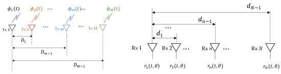
Figure 1.
The arrangement of linear arrays: transmit elements (left) and receive elements (right).
The transmission signal in the θ direction can be expressed by
where is a wavenumber, is the array pattern of each transmit element, and the superscript T denotes the operation of matrix transpose. Then, the target reflection signal in the direction is
where is the complex reflection coefficient, is the delay by the target distance, and is the white gaussian noise. The output of the receiver arrays is:
where . Each transmit waveform is separated by matched filtering with . The output of a matched filter by the m-th waveform is:
where * denotes the complex conjugate, is the m-th element of the vector in Equation (2), and is the interference, including noise and the sum of correlations between and the other waveforms. The final MIMO-received signal vector of length NM is represented as follows:
where stands for the Kronecker product. This shows that the structure of VAA is determined by . If the spacing among the elements is uniform, such as
it is known that the largest aperture can be made when or . If then
which shows that a large aperture of length can be made with a small number of arrays, . Therefore, this allows the HFSWR to improve the azimuth angle resolution. In addition, the output of a beamformer with a complex weight vector is represented by
where H stands for conjugate transpose. It means that the final beamwidth is also dependent on the beamforming weight. The output is affected by the characteristics of the interference . If the waveforms are orthogonal with each other, in Equation (6) includes only the noise component, and the best signal-to-noise ratio (SNR) improvement can be expected by the matched filter and beamformer. However, if they are not matched, the output SNR deteriorates and the detection performance degrades. In summary, the three issues of MIMO are the arrangement of the arrays, beamforming weights, and the waveforms. The following section describes the orthogonal codes of waveforms.
2.2. Orthogonal Polyphase Codes
Orthogonal sequences have been widely studied for wireless communication systems to mitigate interference and increase data capacity. Typically, two sequences are considered orthogonal if the sum of their element-wise products, that is, their dot product, is zero. However, if not synchronized, as in radar systems, the orthogonality depends on the relative shift of the two sequences and is involved in the cross-correlation operation. Reference [32] studied and surveyed sequences with the desired cross-correlation function. Here, we summarize how to get the orthogonal polyphase code set from the complementary pairs and the Hadamard matrix from Ref. [33].
Complementary codes are sets of sequences characterized by the property that for corresponding shifts, the sum of the autocorrelations of the sequences is zero, except for the main peak at the zero shift. A specified length of code can be recursively derived from shorter length codes. Assume a polyphase complementary pair with phases and length N as follows:
Then, the pair of length can be derived from the two complementary pairs of lengths, X and Y. For example, from the two complementary pairs and of length 3, the pairs of length 18 can be found.
where ⊗ represents the Kronecker product. Here are two quad-phase complementary codes of length 3.
From Equation (13), the 18-length complementary pair can be calculated as follows:
This pair can create the Hadamard matrix H, where the row vectors are orthogonal code sets of length 36.
where and are the elements of and in Equations (16) and (17).
- If the p-th row vector of H is written as
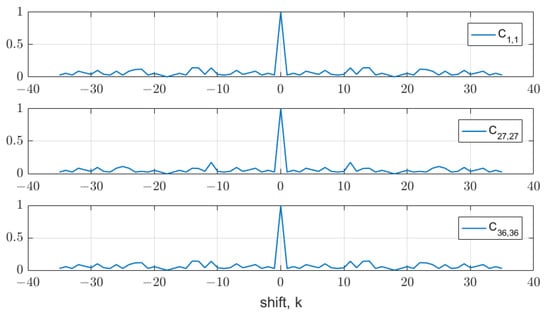
Figure 2.
Autocorrelation function of 1, 27, and 36 codes.
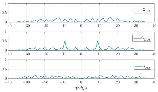
Figure 3.
Cross-correlation function of 1, 27, and 36 codes.
If these codes are used as intra-pulse modulation, they are orthogonal only at the target position, that is, . However, in the surroundings where k is not zero, the interference increases by the autocorrelation and cross-correlation functions, making detection difficult. Therefore, several studies have proposed design methods to minimize these interferences for all k, even if they are not orthogonal at any point [21,22,23]. However, as the concurrently used codes increase, the interference inevitably grows. If the input R is defined as the sum of P different codes, the output from the correlator using the code can be represented as follows:
Figure 4 shows the average level of the sidelobe of as the number of codes, P, increases, when using the codes of the H matrix in Equation (18). Each value was normalized by the code length, and was used as the correlator. Although the values are different depending on the code used as a correlator and the order in which codes are added, it is clear that the levels will increase with the number of codes. This result demonstrates the limitations of employing intra-pulse modulation for MIMO radar.
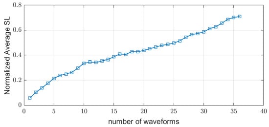
Figure 4.
The average sidelobe level tends to increase with the number of waveforms.
On the other hand, when using pulse-to-pulse modulation, no code shifts occur unless it is the multiple-time-around echo. Figure 5 describes the intra-pulse and inter-pulse modulations. Instead, the Doppler shift of a fast-moving target can cause phase changes among pulses, which leads to code mismatches and orthogonality breakdowns. Figure 6 shows the correlation between the codes, that is, the dot product. When the Doppler shift is zero, the value is zero; otherwise, it is not zero.
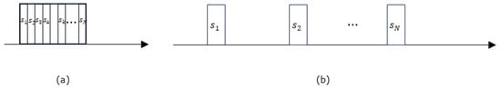
Figure 5.
Intra-pulse modulation (a) and inter-pulse modulation (b).
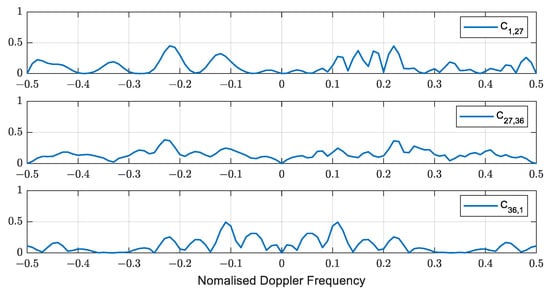
Figure 6.
The orthogonality cannot be maintained due to the Doppler shift.
If the Doppler shift is small, like in HFSWR systems, this type of modulation is quite effective. The subsequent section quantifies the features of HFSWR and proposes an efficient pulse-to-pulse modulation method.
3. HFSWR and the Proposed Method
3.1. HFSWR System
The HFSWR is an economical solution for over-the-horizon surveillance. The lower band of 3−5 MHz is primarily used for long-range surveillance because, as the frequency increases, the propagation loss increases.
Due to its limited instantaneous bandwidth and long wavelength, the HFSWR has a low range and angular resolution. The available instantaneous bandwidth is typically less than 40 kHz, resulting in a coarse-range resolution of more than 3.75 km. When using an operating frequency of 3 MHz, the wavelength is 100 m. So, even if the aperture of the antenna reaches 1 km, the angular resolution is approximately 0.1 rad, and the cross-range resolution at 200 NM is more than 37 km. However, this implies that the target remains in the same resolution cell for a long time, enables long integration times, and results in high-velocity resolution. For example, the traversal time of a ship at 40 knots across the resolution cell of 3.75 km is about 182 s. In addition, most ship targets have low Doppler frequencies of 1 Hz or less at an operating frequency of 3 MHz. A ship traveling at 40 knots (20.6 m/s) has a Doppler frequency of approximately 0.412 Hz.
A pulse repetition frequency (PRF) is typically selected by considering the maximum detection range and Doppler frequency. A PRF that covers the maximum range without causing velocity ambiguity should satisfy the following inequalities:
where is the maximum detection range, is the pulse width, c is the speed of light, and is the maximum Doppler frequency. If a duty cycle of 10% is assumed, the PRF satisfying the above conditions lies in the range of 2 to 360 Hz. In other words, an HFSWR system can choose PRFs from a very wide range. As long as the overall integration time and duty cycle are maintained, the choice of PRF would not affect the velocity resolution or SNR. Rather, using a high PRF increases the number of coherent integration pulses up to tens of thousands because the integration time required for sufficient velocity resolution is tens of seconds. It requires high computational power. Therefore, we propose a novel method to reduce the coherent integration pulses while using a high PRF for MIMO multiplexing.
3.2. LFM and Orthogonal Code Modulation
The proposed method uses a high PRF but with fewer coherent integration pulses by combining a few pulses using correlators. The code length can be selected such that the Doppler processing interval is sufficiently small to avoid velocity ambiguity. This also ensures a small phase mismatch due to the Doppler shift within the code modulation.
Figure 7 describes input samples from one receiver. A transmitter modulates consecutive LFM pulses with orthogonal polyphase codes, . In other words, every pulse has the same LFM waveform with a specified initial phase. The subscript p represents the code number as well as the transmitter number.
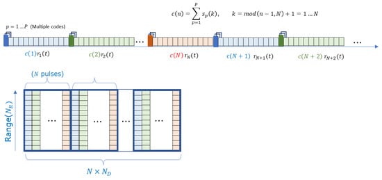
Figure 7.
Description of the received samples in one receiver.
The received sample can be represented as the sum of the transmitted codes, , multiplied by the pulse return signal, . The pulse return signal can be replaced by the first return and the Doppler shift as follows:
where is the Doppler frequency of a moving target and is the pulse repetition interval (PRI). The function returns a remainder after division, so the range is from to . The size of input data is defined as the number of range bins, , and the total number of pulses :
The processing in one receiver starts with pulse compression. The pulse compression is performed for each pulse return by an LFM-matched filter. After that, the correlator separates the transmit codes with N successive pulses. A correlator multiplies each pulse with a specified code and accumulates them. The size of the output data from each correlator therefore reduces to . Finally, the Doppler processing using pulse samples is carried out. Figure 8 shows the whole processing chain.
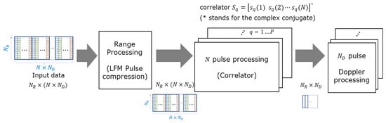
Figure 8.
Signal processing of the proposed method.
The output of the correlator q can be expressed as follows:
where q is the correlator number and is the repetitive number of the code. The first term of Equation (26) is the autocorrelation, while the second term is the sum of the cross-correlation functions, when there is no code shift. If , the first term is N, and the second term is zero by the orthogonality. Even when is not zero, the phase shifts are expected to be sufficiently small to maintain a little cross-correlation.
The advantage of the proposed method and the effect can be observed using the ambiguity function. The correlation function of the phase codes in the previous section changes very little within the velocity of interest, so using intra-pulse modulation produces an ambiguity function shown in Figure 9. The figure on the left is part of a well-known ambiguity function for a phase code, using code 1 in the simulation. Note that only the Doppler frequency, that is, a narrow range of velocity, is represented. On the right is the cross-ambiguity function of codes 1 and 36, which also shows little change in the velocity direction.
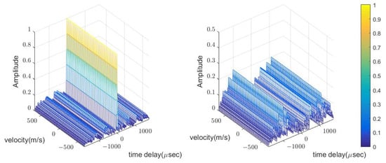
Figure 9.
The ambiguity function of code 1 and the cross-ambiguity function of codes 36 and 1 when using the intra-pulse modulation.
On the other hand, the result of the matched filter and the correlator of the proposed method have the ambiguity function shown in Figure 10. The ambiguity function in the first plot is similar to that of an LFM-matched filter. Also, it rarely varies in the velocity region of interest, although it decreases by the correlator as the velocity increases. The second and third plots show the cross-ambiguity function of codes 1 and 36. Compared with that of the intra-pulse modulation, it is very small in both range and velocity directions, especially in the region of interest, which shows a very low interference level. The maximum velocity of interest is indicated in the third plot.
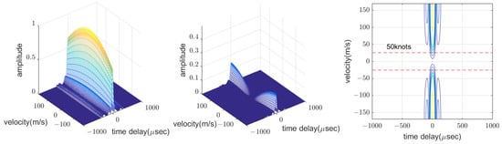
Figure 10.
The ambiguity function of code 1 and the cross-ambiguity function of codes 36 and 1 using the proposed method.
In addition, the proposed method does not introduce the code shift because the maximum detection range is within a PRI and the code is constant for a PRI. Instead, multiple-time-around echoes with the shifted code are removed automatically. Unwanted second-time-around echoes in the HFSWR system include ionospheric clutter, and the ability to remove them is also simulated later.
3.3. Doppler Insensitive Code Selection
To analyze the effect of the Doppler frequency , we define the interference quotient as the ratio of the second term in Equation (26) (the cross-correlation) to the first term (the autocorrelation) in each correlator as follows:
First, is calculated as the number of codes P increases in order from the first row using the first 10 rows of H. Figure 11 shows that when the velocity is zero, is zero, even if the number of waveforms increases. It is because of the orthogonality among the codes. When the velocity is not zero, the values are small, less than 5%. The increase in interference is more significant owing to the increase in target velocity than the increase in the number of waveforms.
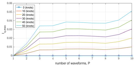
Figure 11.
The increase in interference quotient is more significant with the increase in target velocity than with the increase in the number of transmit waveforms.
Next, we select a Doppler-insensitive transmit code set by finding the code that minimizes the above interference quotient . Table 1 lists the optimized sets, and Figure 12 shows the results. With the selected set, the interference is very low, even at higher speeds or with a large number of codes. The maximum interference level at 50 knots is less than 2.5%, and less than 1% when using four or fewer codes.

Table 1.
Optimized code sets.
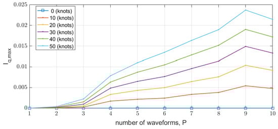
Figure 12.
The interference quotient is reduced by the Doppler-insensitive code selection.
4. Simulation
The orthogonal codes and the structure suggested in the previous sections were used to simulate an HFSWR detection. The operating frequency was 3 MHz, the PRF was 250 Hz, the pulse width was 400 µs, and the LFM of a 20 kHz bandwidth was modulated within the pulse. The total number of pulses was 9216; the code was modulated in 36 successive pulses, while 256 outputs of the correlators were used for Doppler processing.
4.1. Comparison with Intra-Pulse Modulation
In this section, we compare the interference levels of the proposed method with the case of code multiplexing with intra-pulse modulation. The intra-pulse modulation was performed with the same codes, and the single code duration was 50 µs to meet the same instantaneous bandwidth of 20 kHz. The pulse width was 1.8 ms, the PRI was adjusted to 18 ms to maintain a 10% duty, and the number of pulses was 2048 for the same velocity resolution. The conventional range and Doppler processing were performed, and the codes were used as matched filters.
Figure 13 shows the processing results of the two correlators for a target signal moving at 50 knots at 225 km. A single transmit code was used to compare the correlator outputs. Correlator 1 used the same code as the transmit code, whereas correlator 2 used the other. The transmit code was code 1, the first-row vector of H in Equation (18), and the other was code 27. The outputs of the two correlators exhibited high-range sidelobes, and they remain in the final range-Doppler (RD) map. Figure 14 shows the range profile of the target signal, which also exhibits poor range sidelobe characteristics.
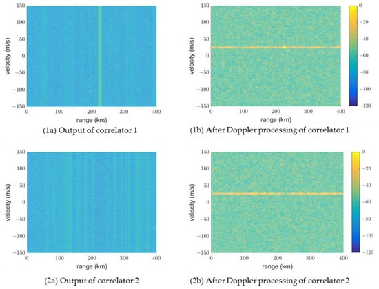
Figure 13.
The range-sidelobe is high when performing code modulation within a pulse.
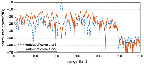
Figure 14.
Range profiles of target signal from RD maps (1b) and (2b) in Figure 13.
Next, we present the results obtained by applying the proposed method in Figure 8. Because each pulse was an LFM waveform, the inputs were first processed using the matched filter. Subsequently, every 36 pulses were correlated with a code. The target signal disappeared when it passed through a correlator with a different code. Figure 15 and Figure 16 show that the sidelobes by multiple codes do not appear in the range or the Doppler direction. As well, the range sidelobes of an LFM could be further reduced using windows.
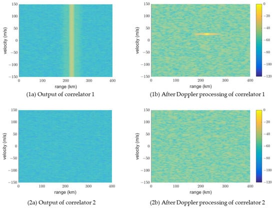
Figure 15.
Compared with the intra-pulse modulation method, the sidelobe in the range direction disappears, and the interference output from correlator 2 is very low.
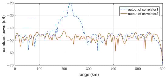
Figure 16.
Range profiles from RD maps (1b) and (2b) in Figure 15.
4.2. Effect of Removing Second-Time-around Echo
Ideally, the HFSWR uses transmission waves that travel entirely along the ocean surface [34]. However, the transmitting antenna radiates partial energy to the elevation, while the pattern of the vertically polarized receiving arrays has some overhead gain. Therefore, a partial wave that radiates upward and is reflected from the ionosphere is unavoidable. The echo at the receiving antennae from various paths is called ionospheric clutter. The path of the ionospheric clutter includes the sky-wave path (including vertical and oblique propagation) and the mixed path (via the ocean surface path). The oblique sky-wave path or mixed path can be longer than the maximum detection range and cause second-time-around echoes. Ionospheric clutter often spreads in the Doppler and spatial domains [35].
We simulated the second-time-around echo signal by multiple scatters at an apparent distance of 200 km, spreading in the Doppler direction. Figure 17 shows the range-Doppler map in a typical pulsed Doppler radar: These echo signals should be resolved through additional measurements or algorithms. However, if a second or multiple-time-around echo occurs, it can be automatically removed using the proposed method, as shown in Figure 18. That is because in the case of a multiple-time-around echo, the received pulse code is shifted by the multiplicity, and thus the autocorrelation is very low, as shown in Figure 2.
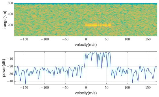
Figure 17.
Example of a second-time-around echo at 200 km of apparent range.
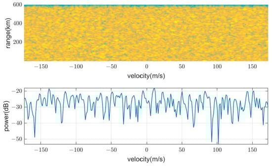
Figure 18.
Removing the second-time-around echo by inter-pulse modulation.
4.3. Improvement of Angle Resolution via Virtual Array Antenna
Finally, we performed virtual array processing by applying the proposed method. The beamforming is performed after the whole processing of Figure 8. Figure 19 shows the configuration of a co-located MIMO antenna. It comprises four receive arrays spaced by , half a wavelength, and three transmit arrays spaced by the receiver antenna’s length, which simultaneously transmit three different waveforms. Then, the synthesized virtual antenna becomes 12 uniform arrays with space. The transmit codes were 1, 27, and 36 row vectors of H, and the waveform parameters were the same as in the previous section. The angular estimation performance may change depending on the beamforming method. Here, we used the typical phase alignment weight for 12 virtual arrays. That means the complex weight in Equation (9) was selected as .
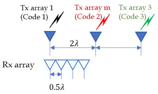
Figure 19.
Co-located MIMO structures of transmit and receive arrays.
Monte Carlo simulations were conducted for a target moving at a velocity of 20 m/s (39 knots) in a direction of 10 degrees. To see the effect of interferences, we performed the case with a range mismatch, where the mismatch interval is 40 microseconds, or 60% of the one-code duration used for intra-modulation. The resulting beam patterns are shown in Figure 20.
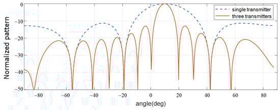
Figure 20.
Beam patterns using a single transmitter and three transmitters.
Figure 21 shows the root mean square (RMS) error as a function of the input SNR of each element. The proposed method outperforms intra-pulse modulation to estimate the angle.
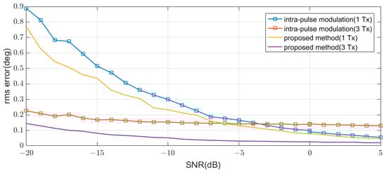
Figure 21.
Comparison of the angular accuracy of the proposed method and the intra-pulse modulation method.
The interference of the significant cross-correlation degrades the performance of the intra-pulse modulation schemes. It becomes more pronounced as the SNR increases because the cross-correlations among signals also grow with the signal power. Therefore, the measurement error cannot fall below a specific value, determined by the cross-correlation value. In other words, even if the angular resolution increases due to the increase in VAA aperture, the accuracy is limited by the signal-to-interference ratio (SIR). However, by employing the proposed method, the cross-correlation is significantly reduced, resulting in a substantial improvement in measurement accuracy.
5. Conclusions
This paper proposes a practical MIMO waveform and processing that can be used in HFSWRs for over-the-horizon detection. The proposed method involved dual modulation using LFM waveforms within the pulse and orthogonal polyphase codes for a few consecutive pulses to enable MIMO processing. Although the orthogonal phase codes were designed simply from the Hadamard matrix, compared with other complex optimization algorithms that consider sidelobes of auto- and cross-correlation functions, their performance was excellent. This was due to the Doppler characteristics of the HFSWR, though its applicability for other radars might be limited. Simulations demonstrated that the proposed method is practical and effectively removes mutual interference. It also showed excellent performance in the removal of multiple-time-around echo-like ionospheric clutter in HFSWR systems. Finally, we showed that MIMO VAA using the proposed method improved the angular accuracy.
This paper applied the proposed method to co-located radar systems, but we anticipate that it could be applied to widely separated MIMO systems.
Author Contributions
Conceptualization, E.K. and S.S.; methodology, E.K.; validation, H.M. and J.H.C.; formal analysis, E.K.; investigation, E.K.; resources, H.M. and K.L.; writing—review and editing, E.K. and S.S. All authors have read and agreed to the published version of the manuscript.
Funding
This research received no external funding.
Data Availability Statement
Data are contained within the article.
Acknowledgments
This was performed based on the cooperation with Sejong university—LIG Nex1 Cooperation.
Conflicts of Interest
Authors S.S., H.M., J.H.C. and K.L. were employed by the LIGNex1 Co. The remaining authors declare that the research was conducted in the absence of any commercial or financial relationships that could be construed as a potential conflict of interest.
References
- Sun, W.; Ji, M.; Huang, W.; Ji, Y.; Dai, Y. Vessel tracking using bistatic compact HFSWR. Remote Sens. 2020, 12, 1266. [Google Scholar] [CrossRef]
- Ponsford, T.; Wang, J. A review of high frequency surface wave radar for detection and tracking of ships. Turk. J. Electr. Eng. Comput. Sci. 2010, 18, 409–428. [Google Scholar] [CrossRef]
- Ponsford, A.M.; Dizaji, R.M.; Mckerracher, R. HF surface wave radar operation in adverse conditions. In Proceedings of the International Conference on Radar (IEEE Cat. No. 03EX695), Adelaide, SA, Australia, 3–5 September 2003; IEEE: Piscataway, NJ, USA, 2003; pp. 593–598. [Google Scholar]
- Headrick, J.M.; Stuart, J.A.; Merrill, S. HF over-the-horizon radar. In Radar Handbook; McGraw Hill: New York, NY, USA, 2008; Volume 20. [Google Scholar]
- Zhang, L.; Shi, C.; Niu, J.; Ji, Y.; Wu, Q.J. DOA estimation for HFSWR target based on PSO-ELM. IEEE Geosci. Remote Sens. Lett. 2021, 19, 3504205. [Google Scholar] [CrossRef]
- Chen, Z.; He, C.; Zhao, C.; Xie, F. Enhanced target detection for HFSWR by 2-D MUSIC based on sparse recovery. IEEE Geosci. Remote Sens. Lett. 2017, 14, 1983–1987. [Google Scholar] [CrossRef]
- Greiff, C.; Giovanneschi, F.; Gonzalez-Huici, M.A. Matrix pencil method for DoA estimation with interpolated arrays. In Proceedings of the 2020 IEEE International Radar Conference (RADAR), Washington, DC, USA, 28–30 April 2020; pp. 566–571. [Google Scholar]
- Zheng, G.; Chen, C.; Song, Y. Height Measurement for Meter Wave MIMO Radar based on Matrix Pencil Under Complex Terrain. IEEE Trans. Veh. Technol. 2023, 72, 11844–11854. [Google Scholar] [CrossRef]
- Yilmazer, Y.; Sarkar, T.K. Efficient computation of the azimuth and elevation angles of the sources by using unitary matrix pencil method (2-d ump). In Proceedings of the 2006 IEEE Antennas and Propagation Society International Symposium, Albuquerque, NM, USA, 9–14 July 2006; pp. 1145–1148. [Google Scholar]
- Xiao, J.J.; Nehorai, A. Optimal polarized beampattern synthesis using a vector antenna array. IEEE Trans. Signal Process. 2008, 57, 576–587. [Google Scholar] [CrossRef]
- Chintagunta, S. Joint 2D-DOA estimation of coherent targets using EV sensors in MIMO radar. Signal Process. 2022, 201, 108715. [Google Scholar] [CrossRef]
- Wen, F.; Shi, J.; Gui, G.; Gacanin, H.; Dobre, O.A. 3-D positioning method for anonymous UAV based on bistatic polarized MIMO radar. IEEE Internet Things J. 2022, 10, 815–827. [Google Scholar] [CrossRef]
- Liu, A.; Zhang, X.; Yang, Q.; Deng, W. DOA estimation with extended sparse and parametric approach in multi-carrier MIMO HFSWR. J. Eng. 2019, 21, 7810–7814. [Google Scholar] [CrossRef]
- Donnet, B.J.; Longstaff, I.D. MIMO radar, techniques and opportunities. In Proceedings of the 2006 European Radar Conference, Manchester, UK, 13–15 September 2006; IEEE: Piscataway, NJ, USA, 2006; pp. 112–115. [Google Scholar]
- Frazer, G.J.; Abramovich, Y.I.; Johnson, B.A.; Robey, F.C. Recent results in MIMO over-the-horizon radar. In Proceedings of the 2008 IEEE Radar Conference, Rome, Italy, 26–30 May 2008; pp. 1–6. [Google Scholar]
- Lesturgie, M. Some relevant applications of MIMO to radar. In Proceedings of the 2011 12th International Radar Symposium (IRS), Leipzig, Germany, 7–9 September 2011; IEEE: Piscataway, NJ, USA, 2011; pp. 714–721. [Google Scholar]
- Frazer, G.J.; Abramovich, Y.I.; Johnson, B.A. Spatially waveform diverse radar: Perspectives for high frequency OTHR. In Proceedings of the 2007 IEEE Radar Conference, Waltham, MA, USA, 17–20 April 2007; IEEE: Piscataway, NJ, USA, 2007; pp. 385–390. [Google Scholar]
- Willis, N.J. Bistatic Radar; SciTech Publishing: Raleigh, NC, USA, 2005. [Google Scholar]
- Riddolls, R.J. A Canadian Perspective on High-Frequency Over-the-Horizon Radar; Technical Report. DREO TR 285; Defense Research Development Canada: Ottawa, ON, USA, 2006.
- Daum, F.; Huang, J. MIMO radar: Snake oil or good idea? IEEE Aerosp. Electron. Syst. Mag. 2009, 24, 8–12. [Google Scholar] [CrossRef]
- Kim, E.H.; Kim, K.H. Random phase code for automotive MIMO radars using combined frequency shift keying-linear FMCW waveform. IET Radar Sonar Navig. 2018, 12, 1090–1095. [Google Scholar] [CrossRef]
- Blunt, S.D.; Mokole, E.L. Overview of radar waveform diversity. IEEE Aerosp. Electron. Syst. Mag. 2016, 31, 2–42. [Google Scholar] [CrossRef]
- Li, J.; Stoica, P. MIMO radar with colocated antennas. IEEE Signal Process. Mag. 2007, 24, 106–114. [Google Scholar] [CrossRef]
- Deng, H.; Geng, Z.; Himed, B. MIMO Radar Waveform Design for Transmit Beamforming and Orthogonality. IEEE Trans. Aerosp. Electron. Syst. 2016, 52, 1421–1433. [Google Scholar] [CrossRef]
- Liu, B. Orthogonal discrete frequency-coding waveform set design with minimized autocorrelation sidelobes. IEEE Trans. Aerosp. Electron. Syst. 2009, 45, 1650–1657. [Google Scholar] [CrossRef]
- Yu, C.; Chang, G.; Ji, Y.; Wang, Y.; Liu, A. DFCW-LFM analysis for MIMO HFSWR. In Proceedings of the 2016 CIE International Conference on Radar (RADAR), Guangzhou, China, 10–13 October 2016; IEEE: Piscataway, NJ, USA, 2016; pp. 1–5. [Google Scholar]
- Khan, H.A.; Edwards, D.J. Doppler problems in orthogonal MIMO radars. In Proceedings of the 2006 IEEE Conference on Radar, Verona, NY, USA, 24-27 April 2006; pp. 244–247. [Google Scholar]
- Kim, E. MIMO FMCW Radar with Doppler-Insensitive Polyphase Codes. Remote Sens. 2022, 14, 2595. [Google Scholar] [CrossRef]
- Linwei, W.; Bo, L.; Changjun, Y.; Zhe, L. LFM-CCC orthogonal waveform design for MIMO-HFSWR. In Proceedings of the IET International Radar Conference (IET IRC 2020), Online, 4–6 November 2020; pp. 481–487. [Google Scholar]
- Chang, G.; Liu, A.; Yu, C.; Ji, Y.; Wang, Y.; Zhang, J. Orthogonal waveform with multiple diversities for MIMO radar. IEEE Sens. J. 2018, 18, 4462–4476. [Google Scholar] [CrossRef]
- Bergin, J.; Guerci, J.R. MIMO Radar: Theory and Application; Artech House: Norwood, MA, USA, 2018. [Google Scholar]
- Velazquez-Gutierrez, J.M.; Vargas-Rosales, C. Sequence sets in wireless communication systems: A survey. IEEE Commun. Surv. Tutor. 2016, 19, 1225–1248. [Google Scholar] [CrossRef]
- Frank, R.L. Polyphase Complementary-Codes. IEEE Trans. Inf. Theory 1980, 26, 641–647. [Google Scholar] [CrossRef]
- Ji, X.; Li, J.; Yang, Q. Annual Characteristic Analysis of Ionosphere Reflection from Middle-Latitude HF Over-the-Horizon Radar in the Northern Hemisphere. IEEE Trans. Geosci. Remote Sensing. 2023, 61, 5104117. [Google Scholar] [CrossRef]
- Yang, X.; Lie, A.; Yu, C.; Wang, L. Ionospheric Clutter model for HF Sky-wave path propagation with an FMCW source. Int. J. Antennas Propag. 2019, 2019, 1782942. [Google Scholar] [CrossRef]
Disclaimer/Publisher’s Note: The statements, opinions and data contained in all publications are solely those of the individual author(s) and contributor(s) and not of MDPI and/or the editor(s). MDPI and/or the editor(s) disclaim responsibility for any injury to people or property resulting from any ideas, methods, instructions or products referred to in the content. |
© 2023 by the authors. Licensee MDPI, Basel, Switzerland. This article is an open access article distributed under the terms and conditions of the Creative Commons Attribution (CC BY) license (https://creativecommons.org/licenses/by/4.0/).