Article

A Multi-Pixel Split-Window Approach to Sea Surface Temperature Retrieval from Thermal Imagers with Relatively High Radiometric Noise: Preliminary Studies

1
Consiglio Nazionale delle Ricerche, Istituto di Scienze Marine (ISMAR-CNR), 00133 Rome, Italy
2
Department of Biological Sciences, University of South Carolina, Columbia, SC 29208, USA
*
Author to whom correspondence should be addressed.
Remote Sens. 2023, 15(9), 2453; https://doi.org/10.3390/rs15092453
Submission received: 28 February 2023 / Revised: 21 April 2023 / Accepted: 2 May 2023 / Published: 6 May 2023
(This article belongs to the Special Issue Atmospheric Correction of Remote Sensing Imagery)

Abstract

:
In the following decade(s), a set of satellite missions carrying thermal infrared (TIR) imagers with a relatively high noise equivalent differential temperature (NEdT) are expected, e.g., the high resolution TIR imagers flying on the future Thermal infraRed Imaging Satellite for High-resolution Natural resource Assessment (TRISHNA), Land Surface Temperature Monitoring (LSTM) and NASA-JPL/ASI Surface Biology and Geology Thermal (SBG) missions or the secondary payload on board the ESA Earth Explorer 10 Harmony. The instruments on board these missions are expected to be characterized by an NEdT of ⪆0.1 K. In order to reduce the impact of radiometric noise on the retrieved sea surface temperature (SST), this study investigates the possibility of applying a multi-pixel atmospheric correction based on the hypotheses that (i) the spatial variability scales of radiatively active atmospheric variables are, on average, larger than those of the SST and (ii) the effect of atmosphere is accounted for via the split window (SW) difference. Based on 32 Sentinel 3 SLSTR case studies selected in oceanic regions where SST features are mainly driven by meso to sub-mesoscale turbulence (e.g., corresponding to major western boundary currents), this study documents that the local spatial variability of the SW difference term on the scale of ≃3 × 3 km2 is comparable with the noise associated with the SW difference. Similarly, the power spectra of the SW term are shown to have, for small scales, the behavior of white noise spectra. On this basis, we suggest to average the SW term and to use it for the atmospheric correction procedure to reduce the impact of radiometric noise. In principle, this methodology can be applied on proper scales that can be dynamically defined for each pixel. The applicability of our findings to high-resolution TIR missions is discussed and an example of an application to ECOSTRESS data is reported.

1. Introduction

The retrieval of the sea surface temperature (SST) from space is a well-consolidated remote sensing activity, and derived products are used in several operational applications [1]. Currently, and for the foreseeable future, global ocean operational SST retrieval is based on measurements from a set of ad hoc instruments, such as VIIRS [2], SLSTR [3] and METIMAGE [4]. Generally, SST retrieval involves state-of-the-art atmospheric correction algorithms based on the split window (SW) method (see, e.g., [5,6]), that exploit observations from two or three atmospheric channels and, in some cases (e.g., SLSTR and A-ATSR), from dual view observations [7]. Alternatively, SST retrieval is based on the Optimal Estimation Method (OEM) [8].
SST applications require very low uncertainty of the estimated value (<0.1 K), and the requirements for the instruments and processing algorithms to fulfil such a condition are stringent in terms of channel co-registration, radiometric characteristics and the accuracy of the inversion algorithm.
Besides the state-of-the-art instruments dedicated to SST retrieval, other instruments with weaker radiometric and geometrical performance are equipped with channels that can be used for SST estimation. The consequent lower quality of the retrieved products may be derived by the secondary payload nature of the instrument (e.g., CALIPSO-IIR [9] and HARMONY thermal infrared (TIR) payload [10,11,12]) or by the high spatial resolution (HR) of the instrument (e.g., ASTER [13], ECOSTRESS [14] and LANDSAT8-9 [15,16]). In particular, within the next few years, there are several satellite missions planned to launch HR TIR sensors that, although mostly dedicated to land applications, will acquire data over coastal regions at the very least. Obtaining a high-resolution SST over coastal regions is of interest for coastal process studies, for example, the study of the dynamics of upwelling systems [17], inshore water quality [18] and the thermal discharge of cooling water from nuclear power stations [19].
The aforementioned high resolution missions are:
  • The NASA-JPL/ASI Surface Biology and Geology Thermal Mission (SBG), focusing on five research and applications areas: terrestrial and aquatic ecosystems, hydrology, weather, climate and solid Earth [20].
  • The Thermal infraRed Imaging Satellite for High-resolution Natural resource Assessment (TRISHNA) mission, a cooperation between the French (CNES) and Indian (ISRO) space agencies to launch a satellite in 2025 with a 5-year lifetime to measure the visible, near infrared and thermal infrared signal of the surface atmosphere system globally approximately twice a week, with a 60 m resolution for the continents and coastal oceans and a resolution of 1000 m over deep oceans [21].
  • The Land Surface Temperature Monitoring (LSTM) is an ESA mission set to join the Copernicus Sentinel system in 2028. The satellite will have TIR observation capabilities over land and coastal regions in support of agriculture management services, and possibly a range of additional services. The LSTM mission will consist of two satellites [22].
Table 1 reports the relevant characteristics of a set of past, current and future sensors with relatively high noise equivalent differential temperature (NEdT) in terms of the spectral position of the SW channels and the relevant estimated NEdT values. As a reference, the characteristics of the Sentinel 3 (S3) SLSTR equivalent channels are reported. It should be noted that, in the best of these cases, the NEdT of the reported instruments, excluding the reference SLSTR, is about 0.1 K.
Over oceans, the SW term is proportional to the total amount of water vapour in the atmosphere. Roughly, 1 cm of total precipitable water vapour in the sensed atmospheric path corresponds to 0.5 K of SW difference [23]. For this reason, in conditions of a very dry atmosphere, such as in polar regions, the SW may be dominated by noise, and a single channel correction may be more effective [24]. Besides the extreme case of polar regions, in general, for a given scene (i.e., a geographical region in a given day), the dynamical range of the SW difference is, on average, expected to be around 1 K. Within this frame, it is clear that a NEdT of the order of 0.1 K or higher for the two channels involved in atmospheric correction may induce artefacts in the retrieved SST mostly in the form of a noisy field. As an example, assuming uncorrelated noise, the random uncertainty associated with the SW term can be up to about 0.42 K if both channels have an NEdT of 0.3 K, which is about 40% of the expected range for a given scene.
Since for most of the aforementioned missions the objective is not absolute SST retrieval but rather the identification of structures in the SST field (e.g., gradients and patterns), a noisy SST field results in difficulties in identifying the actual SST patterns. Rather than reducing the noise by smoothing the SST field or using noise robust operators to identify spatial patterns, losing in both cases spatial information, we suggest to explore the possibility of reducing the noise in the atmospheric correction term. This is based on the following hypotheses:
  • The atmospheric correction is based on a functional form that uses the SW difference;
  • The scales of variability of the radiatively active atmospheric components are larger than the spatial sampling distance of the sensor.
A similar approach has been already presented and discussed for SST retrieval by several authors and applied to different instruments.
To reduce the noise in the AVHRR-derived SST based on an SW algorithm, it has been suggested to rely on the average or the median of the SW difference computed over a 3 × 3 [25], 5 × 5 [26] or up to 11 × 11 [27] pixel area.
A similar solution is suggested for SST retrieval from SEVIRI ([28]), discussing the effect of using the average of the SW difference over a 5 × 5 pixel box. In the same study, a strategy to introduce the concept of spatial smoothing also in case of retrieval based on optimal estimation was presented and discussed.
A different approach was suggested in [29,30] for ATSR. In particular, Harris and Saunders [30] proposed to smooth the single pixel ATSR-derived SST ( S S T k , m ) by considering an area around the pixel in the following way:
S S T k , m = B T 11 k , m + i j G i , j ( S S T i , j B T 11 i , j ) i j G i , j
where B T 11 i , j is the 11 μ m brightness temperature (BT) of pixel i , j and G i , j is a cloud-discriminator operator and adopts a value of 0 when the pixel i , j is cloudy and 1 if it is cloud free. The smoothing is estimated as the average of the difference in the single pixel ATSR-derived SST ( S S T i , j ) and the corresponding 11 μ m BT ( B T 11 i , j ). The authors applied smoothing up to a 29 × 29 pixel area (of 1 km size), suggesting that in the above 19 × 19 pixel area there are no significant improvements in noise reduction.
The approach described in Equation (1) was also applied to the SLSTR SST-derived L2P distribution, applying a 3 × 3 pixel kernel (Sea Surface Temperature (SLSTR) Algorithm Theoretical Basis Document, SLSTR-ATBD L2SST-v2.5, October 2012, https://www.eumetsat.int/media/40007, accessed on 29 January 2023).
Finally, the assumption of a relatively low spatial variability of atmospheric properties with respect to surface properties is commonly adopted for similar scales by well-established inversion algorithms for other geophysical variables, for example, for aerosol property retrieval by the Generalized Retrieval of Atmosphere and Surface Properties (GRASP) [31].
This study, independent from the SST retrieval algorithm used in the sensor, focuses on determining under which conditions and scales it is possible to apply an atmospheric correction based on a spatial average of the SW difference to reduce the noise on the final SST field. This will be done by means of real observations from SLSTR instruments on board the Sentinel 3A and 3B satellites.
In order to document the limits of applicability of the proposed approach, a set of SLSTR cases over oceanic regions characterized by the presence of high SST spatial variability was selected. In principle, in the presence of different water masses, as, for example, in the Gulf Stream area, it is likely that an enhanced spatial variability of the lower troposphere results from different air–sea exchanges.
Section 2.1 contains a description of the SLSTR dataset used in this study. In Section 2.2, we present a short review of SST retrieval based on the SW difference with some references relative to the missions of interest. We go on to illustrate the evidences/findings of the proposed methodology in Section 3 and Section 4. Finally, discussions of the results and the main conclusions are provided in Section 5.
Table 1. Examples of spectral and radiometric (NEdT) characteristics of IR channels commonly used for SW computations of interest for this study.
SatelliteBandSpectral Range ( μ m)SSD (m)NEdT (K)
S3-A SLSTRS810.46–11.2410000.014 @ 270K
[3]S911.57–12.4710000.022 @ 270K
Harmony TIRTIR-110.40–11.3010000.150 @ 280 K
[32]TIR-211.40–12.5010000.150 @ 280 K
CALIPSO IIRTIR-210.34–10.9510000.140 @ 250 K
[9]TIR-311.57–11.6210000.110 @ 250 K
ASTERTIR-1310.25–10.9590≈0.120 @ 285 K
[33]TIR-1410.95–11.6590≈0.150 @ 285 K
LANDSAT 8 TIRSCh-1010.6–11.21000.049 @ 300K
[34]Ch-1111.4–12.51000.052 @ 300K
LANDSAT 9 TIRS-2Ch-1010.3–11.31000.080 @ 320K
[35]Ch-1111.5–12.51000.080 @ 320 K
ECOSTRESSCh-510.28–10.69700.110 @ 298 K
[36]Ch-611.80–12.40700.310 @ 298 K
LSTM TIRTIR-410.70–11.10370.150 @ 300 K
[22]TIR-511.76–12.23370.150 @ 300 K
TRISHNATIR-310.25–10.931000 @ Sea0.100 @ 300 K
[21]TIR-411.15–12.031000 @ Sea0.100 @ 300 K
SBGCh-711.04–11.59600.200 @ 275 K
[37]Ch-811.80–12.28600.200 @ 275 K

2. Materials and Methods

2.1. SLSTR Study Cases Data-Set

For our investigation, we relied on the S3 (A and B) Non Time Critical products distributed as L2P SST products by EUMETSAT. These data are compliant with the specifications from the Group for High Resolution Sea Surface Temperature (GHRSST, https://www.ghrsst.org/). They include: (i) L1 single channel Top Of the Atmosphere (TOA) BTs and associated NEdT; (ii) skin SST L2 data and (iii) specific data flags to identify the type and quality of the observations (detailed below). The BTs are provided as observations obtained from the three S3 IR channels S7, S8 and S9, centered at 3.74, 10.85 and 12.02 μ m, respectively.
The l2p_flags variable contains bitmasks that enable the identification and removal of land, ice, lake and river pixels from the L2 data. The quality_level variable which ranges from 0 (no data) to 5 (best quality) was used to identify the best quality (quality_level = 5) pixels. We thus selected BT pixels based on these criteria in order to analyze only high quality, non cloud-contaminated BT observations. These products maintain the original observation geometry of Level 1, i.e., a 1 km Spatial Sampling Distance (SSD) at nadir.

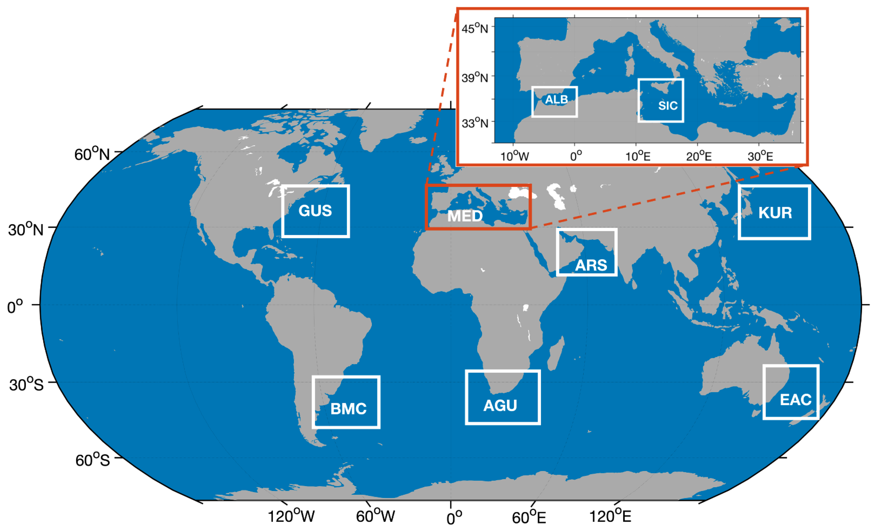
Selection of Study Cases

We focus on oceanic regions where SST features are mainly driven by the meso to sub-mesoscale horizontal/vertical dynamics, thus selecting areas characterized by enhanced eddy activity (i.e., high eddy kinetic energy) [38,39] or upwelling systems [40,41]. This led to the identification of the following areas Of interest (AOI) (Figure 1):
  • Agulhas Current (AGU);
  • Arabian Sea (ARS);
  • Brazil Malvinas Current (BMC);
  • East Australian Current (EAC);
  • Gulf Stream (GUS);
  • Kuroshio Current (KUR);
  • Mediterranean Sea: Alboran Sea (ALB);
  • Mediterranean Sea: Strait of Sicily (SIC).
Such AOIs are often characterized by the presence of fronts due to meandering of the marine surface currents as well as the presence of eddies and filaments [1]. Such a scenario allows us to test the methodology proposed in this study in areas where frontal structures may trigger air–sea interactions, making the SW correction term non-trivial [42]. A visual inspection of each study case was required in order to assure the presence of at least 50% contiguous cloud-free pixels over zones with recognizable frontal/eddy activity.
For each AOI, we selected four study cases in order to account for the different phases of the annual cycle. Table 2 provides detailed information on the set of study cases used in our work.

2.2. Split Window Method

Over oceans, the TOA signal measured from a satellite sensor in the spectral region of interest is, in absence of clouds, dominated by the upwelling radiance emitted by the sea surface, with a contribution due to absorption/emission of the atmosphere. In the majority of cases, the effect of the atmosphere attenuates the radiation emitted by the surface. The SW method is based on different atmospheric absorptions, and therefore on the different measured BTs, in two adequately selected spectral intervals (practically spectral channels) in the IR windows. Typically, the wavebands used for the two channels are in the range of 10.3–11.3 μ m and 11.5–12.5 μ m, respectively [43]. The true SST can be estimated using this difference in an atmospheric correction algorithm, the simplest form of which is:
S S T = a 0 + a 1 B T 11 + a 2 ( B T 11 B T 12 )
where B T 11 and B T 12 are the TOA BTs in the ranges 10.3–11.3 μ m (less contaminated by atmospheric disturbances) and 11.5–12.5 μ m , respectively, and a i are regression coefficients to be determined. More accurate algorithms take into account other terms such as observation geometry, first guess SST values and/or water-vapour-dependent terms (e.g., [44,45,46]). SW-like algorithms developed for SST-dedicated missions (e.g., AVHRR, SLSTR and A-ATSR) have also been used for SST retrieval with high resolution instruments (e.g., ASTER [47], LANDSAT-8 [48] and ECOSTRESS [49]).
Adopting these functional forms, the effective reduction in the retrieval noise by smoothing of the SW term depends upon the specific form of the retrieval equation [50] and the relative magnitudes of the noise levels in the sensor wavelength bands. For example, in the MultiChannel SST algorithm:
S S T = a 0 + a 1 B T 11 + a 2 ( B T 11 B T 12 ) + a 3 S θ ( B T 11 B T 12 )
where S θ = ( s e c ( θ v ) 1 ) , in which θ v is the view zenith angle to account for the observation geometry. If the noise in the two SW channels is uncorrelated, then the noise of the SW term will be larger than the noise of either channel. If the regression coefficient a 2 is > 1 and if a 3 S θ > 1 , then the SW difference term will be amplified by the retrieval equation and smoothing will reduce the retrieval noise to a level close to the a 1 B T 11 noise.

3. Evidence for the Multi-Pixel Approach

To reduce the impact of radiometric noise on the retrieved SST, we explored a multi-pixel approach based on the assumption that the spatial variability of the atmosphere is lower than that of the surface [51,52].
In order to implement such an approach in SW retrieval, we introduce an additional assumption: the atmospheric effect is fully represented by the SW BT differences in the proposed SST retrieval functional form. As an example, Figure 2 shows for a SLSTR Sentinel 3 (S3)-A acquisition over the Kuroshio current area.
(file S3A_SL_2_WST____20210919T232056_20210920T010155_20210921T102504_6059_ 076_272______MAR_O_NT_003):
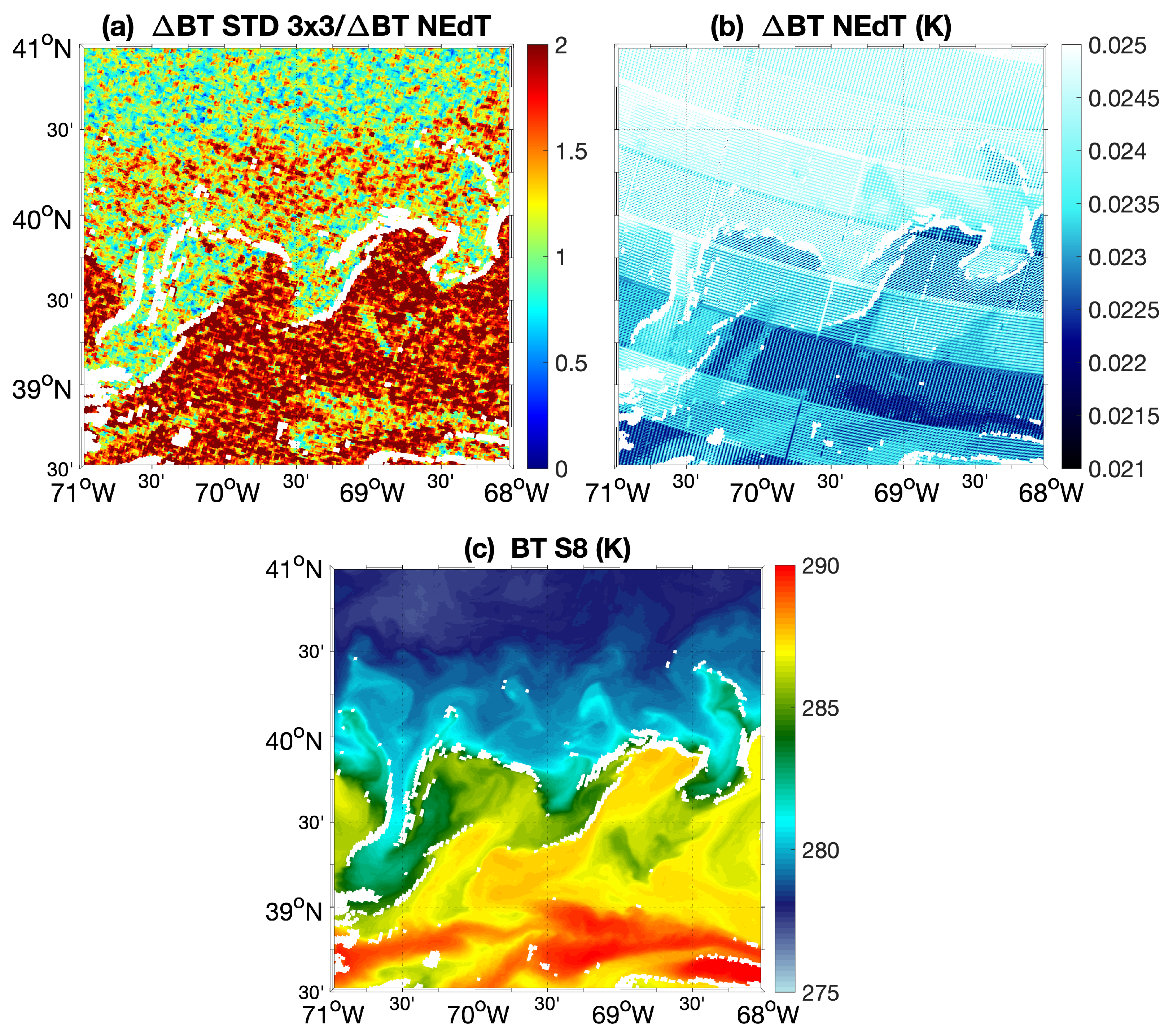
  • The S8 channel TOA BT field, as a proxy for the SST field;
  • The difference between the S8 and S9 channel-derived BTs corresponding to the SW difference ( Δ BT hereinafter);
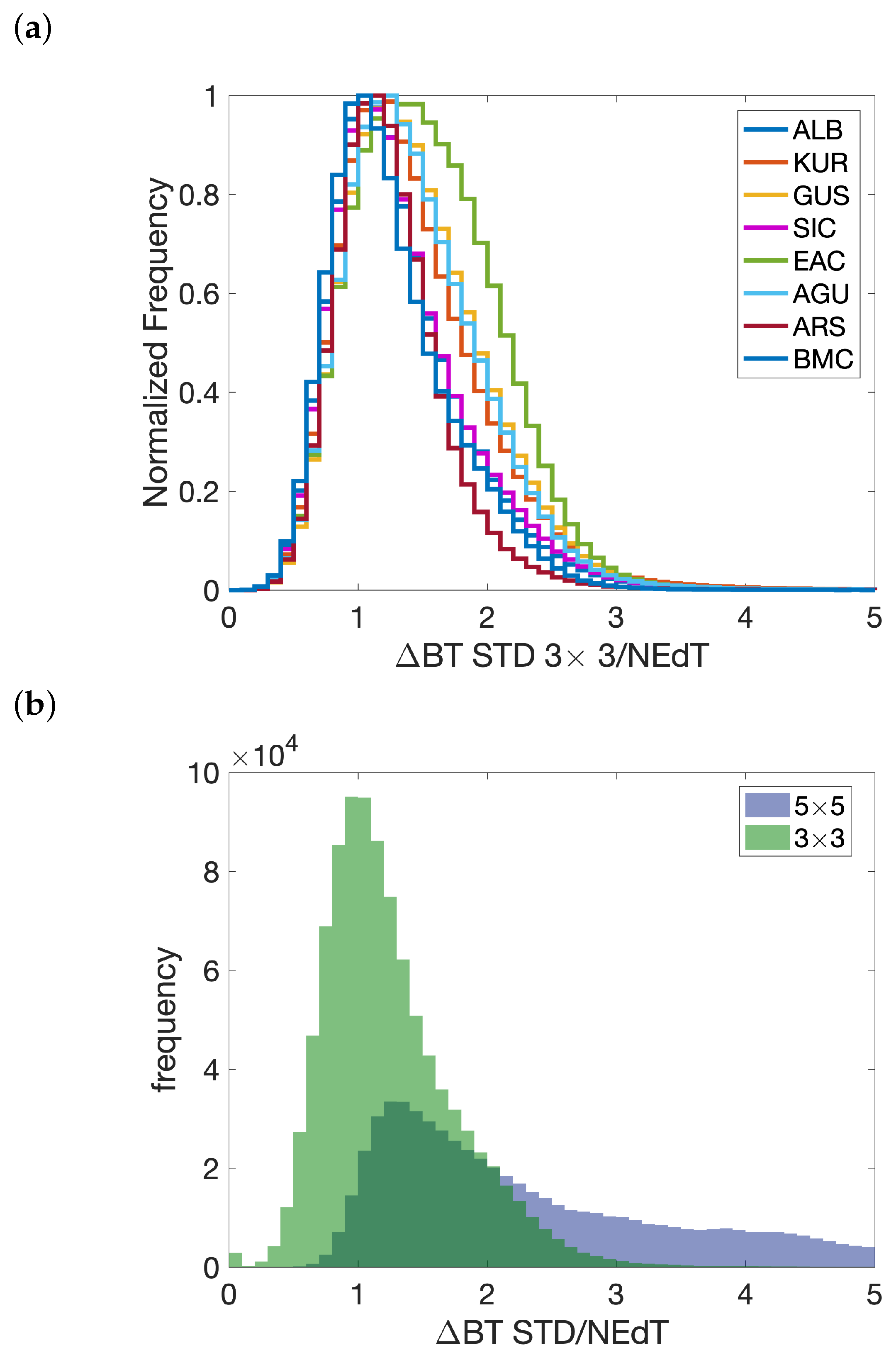
  • The standard deviation over 3 × 3 pixels of the Δ BT;
  • The ratio between standard deviation of the Δ BT and the associated noise. The latter is estimated assuming uncorrelated random noise and using the TOA BT NEdT field for each pixel/band, included in the L2 product [53].
The S8 channel BT exhibits a signature of meso to sub-mesoscale activity, as expected for a western boundary current such as the Kuroshio current. The scene is indeed dominated by mesoscale to sub-mesoscale eddies and filaments, with clearly visible signatures in the SST and hence the TOA BT field (Figure 2a).
The Δ BT term still shows large scale features but appears more noisy, given also the lower range of variability (Figure 2b). The 3 × 3 standard deviation of the Δ BT is on the order of tenths of mK (Figure 2c) and exhibits a local variability of the same order of magnitude of the expected variability due to radiometric noise (Figure 2d). This condition mainly fails in areas characterized by spatial gradients in the original BT signal. Over different water masses, it is likely that the air mass can also be different, particularly on the scale of the example, which partly justifies the occurrence of relatively high values of the standard deviation in the BT difference field. On the other hand, for strong SST gradients, such as the one in the example, spatial features can also be generated by the inter channel co-registration uncertainty that, in the system requirements for SLSTR, should not exceed 0.1 SSD (https://sentinel.esa.int/documents/247904/4755279/S3.PN-SLSTR-L1.09+-+i1r1+-+SLSTR+L1+PB+SL__L1_.004.04.00.pdf). In the case shown in Figure 2, it is thus possible to assume atmospheric homogeneity over a 3 × 3 pixels box, corresponding roughly to an area of about 3 × 3 km 2 . The dimension (in pixels) and shape of the area used to estimate the atmospheric correction should, however, also be a function of the specific scene/sea surface conditions. Corresponding to intense seawater thermal gradients, modulations in the lower atmospheric responses are indeed expected [42,54,55]. This additional investigation is however left for future studies.

4. Results

Based on the study cases detailed in Table 2, we quantified the validity of our assumptions via statistical and spectral analyses.
Figure 3a shows the histogram distribution of the ratio between the local variability of the Δ BT term ( Δ BT STD) and the associated noise (NEdT). As already mentioned in Section 2, the statistics uniquely rely on cloud-free sea pixels. However, to avoid artefacts due to cloud/land contamination, all sea pixels contiguous to a cloudy or land area have not been accounted for. The histograms, reported as normalized frequencies per AOI, peak around the unity value, supporting the hypothesis that the local variability of the atmospheric correction term (over the 3 × 3 km 2 area) is dominated by radiometric noise. For some regions (e.g., EAC), the distribution still peaks around unity, although a slight shift toward larger values can occur.
This is discussed on a test case in the Gulf Stream area, acquired by Sentinel 3B on 30 March 2021 (Figure 4c, file S3B_SL_2_WST____20210330T140133_20210330T154232_20210401T003643_6059_050_352______MAR_O_NT_003), but it was found also for other AOIs such as the EAC.
For this specific scene, the ratio between the 3 × 3 variability of the Δ BT and the associated noise is around 1 north of the main SST front located between 39°N and 40°N, while it increases to 2 south of it (Figure 4a). A closer look at the Δ BT noise field (Figure 4b) [53], as well as the BT from the S8 channel (i.e., our best proxy for SST), evidenced a distinct behavior between the colder and warmer areas in the analyzed test case. In the presence of warmer SSTs, the overall Δ BT noise is reduced and, simultaneously, one can expect a higher atmospheric variability, i.e., an enhancement in the Δ BT standard deviation [42]. These effects can thus contribute to an overall increase in the Δ BT standard deviation/ Δ BT noise ratio. This can also explain the peak displacement of the normalized histograms presented in Figure 3a with respect to unity. However, this is not expected, or at least, not to the same extent, in very high resolution missions such as, e.g., ECOSTRESS, where the NEdT at high temperatures is expected to be significantly larger than for SLSTR.
The assumption of atmospheric homogeneity may fail if we account for areas larger than 3 × 3 km 2 . We thus analyzed a specific case study over the Kuroshio current on the 19 September 2021 (file S3A_SL_2_WST____20210919T232056_20210920T010155_20210921T102504_6059_076_272______MAR_O_NT_003). By imposing homogeneity over a 5 × 5 km 2 area, the distribution of the Δ BT standard deviation divided by the Δ BT NEdT becomes indeed significantly broader and it is not centered around unity, as shown in Figure 3b.
In addition, to further support the assumption on the basis of the multi-pixel approach, we compared the power spectral density (PSD) of the S8 channel BT, the PSD of the Δ BT and the PSD of the Δ BT term averaged by means of a 3 × 3 moving window. The PSD was computed via fast Fourier transform, relying on a Blackman–Harris window to reduce spectral leakage, following [56]. An example of S3A acquisition over the Kuroshio current area (already discussed in Section 3) is depicted in Figure 5.
In particular, the PSD was computed over three cross-sections (white thick lines in Figure 5a). The cross-sections cover approximately 5 longitude degrees and 0.1 latitude degrees, and were chosen to perform the analyses over distinct dynamical regimes of the selected case study:
  • A region with predominance of large-scale patterns at the westernmost and easternmost zones of the scene (cross-section 1);
  • An area with tiny filaments characterized by sharp temperature differences, such as the one located at ≃149.7°E−48.0°N (cross-section 2);
  • An area with much smoother spatial variability (cross-section 3).
The results reported in Figure 5b–d were computed assuming a uniform pixel spacing of 0.015 degrees, the latter was determined as the mean longitudinal spacing in the areas interested by the spectral analysis. Apart from small differences, the three sets of transects yield the same results. The S8 BT (BT8) spectrum exhibits PSDs larger than 10 2 for wavenumbers smaller than 1 deg 1 (scales ≳ 100 km). The PSD progressively decreases for larger wavenumbers and eventually exhibits a flat spectrum, indicating noise, for scales ≲ 2.5 km. The Δ BT (or SW) term PSD is fully compliant with the BT8 one until spatial scales of ≃10 km; the noisy regime is observed immediately afterwards. Such a behavior suggests that the Δ BT term prevents a clear description of spatial features below 10 km, injecting noise even in the retrieval of SST based on SW-like algorithms.
However, considering the findings reported in Section 3 and summarized in Figure 3, we can perform the same spectral analysis after applying a moving 3 × 3 averaging window to the original SW field, with the aim of double checking whether this operation reduces the noise affecting the SW term. This operation makes the Δ BT field spectrally compliant with the S8 channel, reducing the amount of noise in the 10 km to 3 km range. For lower scales, the PSD of the 3 × 3 averaged Δ BT term ( Δ BT 3 × 3 hereinafter) exhibits an abrupt decrease and a subsequent increase, likely due to artefacts introduced by the 3 × 3 averaging. In future studies, this can be further investigated by choosing different averaging kernels. However, this is not expected to affect our analysis, since this occurs in a spectral region where noise dominates both the SW and the S8 field.

5. Discussion and Conclusions

This study approaches the issue of reducing the noise in the atmospheric correction term in multi-spectral regression IR-based SST retrieval algorithms. This approach has been presented and documented by several authors in the past [25,26,27,28,29,30] for state-of-the-art SST-dedicated satellite missions. Within the frame of present day or planned missions with a relatively high NEdT, this methodology can be useful to reduce the noise in the retrieved SST field with advantages for the effective resolution of the estimated SST. Characterization of the main SST frontal features may benefit from such an approach.
The study is based on the hypothesis that the spatial variability of relevant atmospheric variables (mostly temperature and water vapour distribution in the troposphere) is lower than that of the sea surface temperature. In this study, we documented the hypothesis behind the smoothing of the atmospheric correction term by using Sentinel 3 (A/B) SLSTR acquisitions over regions mainly dominated by mesoscale/sub-mesoscale turbulence (e.g., western boundary currents) or those corresponding to major upwelling systems. The aim of this choice was to test the methodology over SST scenes with complex spatial patterns and enhanced frontal activity. The dataset was chosen in order to sample the annual cycle and is characterized by a spatial resolution of ≃1 km. Relying on statistical and spectral analyses, we found the following main results:
  • The local variability of the atmospheric correction term generally employed in split-window algorithms (here referred to as Δ BT), if computed over 3 × 3 km 2 areas, is of the same order of magnitude of the estimated Δ BT radiometric noise;
  • Spectral analyses of the BT, Δ BT and 3 × 3 km 2 averaged Δ BT (performed over a specific study case) suggest that 3 × 3 smoothing on the SW term is helpful in reducing noise in the atmospheric correction procedure and obtaining a SW correction with similar spectral properties to the BT derived from channel S8. This is verified up to scales larger than 3–4 km. It is thus very likely that the SST obtained with the 3 × 3 averaged SW will benefit in terms of noise reduction/effective resolution;
  • The assumption of atmospheric homogeneity over the 3 × 3 km 2 area for the SLSTR case studies was thus supported by our findings. The horizontal extent of the atmospheric homogeneity assumption is, however, a function of the specific satellite mission and should be adapted as a function of the IR sensor SSD and radiometric characteristics.
As shown in some of the examples, there are cases where the local standard deviation of the SW exceeds the noise value expected for the difference. Besides the contamination by clouds and coastlines, which should be reduced by the applied masks, there are other two factors that could be causing this feature observed mostly corresponding to SST gradients:
  • A realistic difference due to the atmospheric response to SST gradients;
  • An artefact due to inter-channel co-registration issues;
In our analyses, the adopted macro-pixel was always a 3 × 3 box independent of the effective spatial variability of the BT fields. The technique should be optimized, particularly for the HR satellite missions (e.g., ECOSTRESS, ASTER, SBG, THRISNA and LSTM).
ECOSTRESS is an example of a high spatial resolution instrument with a high noise level. We used ECOSTRESS L1B Geolocation [57] and L1B Radiance and L2 LST [58] products produced by the NASA Jet Propulsion Laboratory and distributed by the Land Processes Distributed Active Archive Center (LPDAAC, https://lpdaac.usgs.gov). Conversion of radiance to BTs and re-projection of the swath data onto a rectilinear longitude-latitude grid was carried out with the ECOSTRESS_swath2grid Python script provided by LP.DAAC. We analyzed a case study over the Alboran Sea (region ALB in Figure 1) (files listed below):
  • ECOSTRESS_L1B_GEO_17857_004_20210830T022642_0601_01.h5;
  • ECOSTRESS_L1B_RAD_17857_004_20210830T022642_0601_01.h5;
  • ECOSTRESS_L2_LSTE_17857_004_20210830T022642_0601_01.h5.
We used a collocated VIIRS SST retrieval (file 20210830015000-OSPO-L2P_GHRSST-SSTsubskin-VIIRS_N20-ACSPO_V2.61-v02.0-fv01.0.nc) reprojected onto a rectilinear longitude-latitude grid with SeaDAS 8.2.0 software. The ECOSTRESS channel wavelengths were 10.49 μ m and 12.09 μ m, which we used for the BT 10 and BT 11 terms in the SST retrieval equation (3). To establish regression coefficients for the MC SST retrieval algorithm, the 60 pixel regional averages of ECOSTRESS BTs and view zenith angle fields were down-scaled to the VIIRS coordinates with a k-nearest neighbor algorithm. Smoothing was performed by convolving the SW ( Δ BT) fields with 3 × 3 (≃200 × 200 m), 11 × 11 (≃770 × 770 m) and 51 × 51 (≃3.57 × 3.57 km) averaging kernels. BT noise (robust standard deviation), retrieval equation terms, and the retrieved SST were measured with the von Neumann sequential difference method [59]. The noise levels were calculated separately for all rows and columns of the data fields and the median of the row values and column values was used as per image noise estimates. The regression of VIIRS SST against ECOSTRESS predictors was highly significant (R 2 = 0.929, RMSE = 0.475, p < 0.001, df = 3.88327). The coefficients are listed in Table 3. The coefficients associated with the SW terms in the equation (a 2 and a 3 ) were >=1, indicating the potential for amplification of noise by the SW terms during retrieval of the SST [50].
The noise level of the 12 μ m BT was approximately 3 times greater than the noise level of the 11 μ m BT (Table 1). Smoothing greatly decreased the noise level of the SW Δ BT (Table 4 and Figure 6), but had little effect on the noise level of the retrieved SST. This occurred because the noise level of BT11 μ m was much higher than the noise level of the smoothed Δ BT. The high BT11 μ m noise level in ECOSTRESS is largely systematic rather than Gaussian (see Figure 7), and derives from stripes in the images caused by calibration artefacts and non-uniformity of the focal plane array.
However, depending upon the form of the SST retrieval algorithm and its coefficients, in sensors with high noise levels in the primary SST channel (10–11 μ m), smoothing of the split-window terms may not always reduce the retrieval noise. In these cases, other noise mitigation approaches are necessary, including de-striping and direct smoothing of the retrieved SST.
For such missions, in order to obtain an effective noise reduction in the retrieved SST, smoothing should be applied not only to the SW term but also to the BT 11 term. However, based on the assumption of the different scales of variability for oceans and the atmosphere, BT 11 smoothing should be performed over smaller areas, with the objective of maintaining the highest effective resolution possible for the retrieved SST.
The scales of smoothing for each specific sensor and scene should be a trade-off between (i) the noise associated with the measurement, (ii) the sensor SSD and (iii) the target scene effective spatial variability.
Finally, in this work, we adopted a simple square smoothing box. The extent and shape of the smoothing area can be dynamically defined on the basis of the characteristics of the observed field (e.g., [60]).
Finally, it should be noted that for each pixel of the area used to average the SW difference, it is possible to retrieve an SST value. By moving the area for a given pixel, on can obtain different estimates of the SST. For example, in the 3 × 3 pixel cases, up to nine SST values can be obtained for a single pixel. The averages and standard deviations of the SST computed over the set of values relative to a single pixel can be further used as indicators of the robustness of the procedure. In principle, if the hypotheses are correct, the standard deviation of the estimated SST should be on the order of magnitude of the expected noise, as estimated by uncertainty propagation. Deviations from the expected behavior should be analyzed to optimize the procedure.

Author Contributions

Conceptualization, G.L.L. and D.C.; methodology, G.L.L., D.C. and M.S.; software, D.C.; validation, D.C., G.L.L., D.S.W. and M.S.; formal analysis, D.C., G.L.L. and M.S.; investigation, D.C., G.L.L., D.S.W. and M.S.; resources, G.L.L., D.C. and D.S.W.; data curation, D.C. and M.S.; writing—original draft preparation, G.L.L. and D.C.; writing—review and editing, D.C., G.L.L., D.S.W. and M.S.; visualization, D.C. and G.L.L.; supervision, G.L.L.; project administration, G.L.L. and D.C.; funding acquisition, G.L.L. and D.S.W. All authors have read and agreed to the published version of the manuscript.

Funding

This study was funded by TU-DELFT via a subcontract with CNR-ISMAR under the ESA contract no. 4000134959/21/NL/FF/an. D.S.W. was supported by NASA grants 80NSSC20K0074 and NS 80NSSC23K0643.

Data Availability Statement

The Sentinel 3 SLSTR L2P data are freely available via EUMETSAT upon registration via https://navigator.eumetsat.int (accessed on 23 July 2022). VIIRS data are available via podaac.jpl.nasa.gov (accessed on 16 May 2022).

Acknowledgments

A practical contribution to selecting study cases came from Luca Sideri, Aurora Natea, Andrea Bennati, Emanuele Patanè, Matteo Guastini, students of Liceo Scientifico “Pasteur”, Rome, Italy, and from Gianluca Santoro, Martina Giaccaglia, Martina De’Pompeis of Liceo “Chris Cappell College”, Anzio (RM), Italy, within the frame of their stage of PCTO (Percorsi per le Competenze Trasversali e per l’Orientamento), under the coordination of Mara De Meo (Pasteur) and Luciano Burli (Chris Cappell). The students helped in selecting, classifying and documenting cases of interest used in this study. This collaboration with high school students was carried out within the frame of the BlueNights project (https://bluenights.eu/).

Conflicts of Interest

The authors declare no conflict of interest.

References

  1. Minnett, P.; Alvera-Azcárate, A.; Chin, T.; Corlett, G.; Gentemann, C.; Karagali, I.; Li, X.; Marsouin, A.; Marullo, S.; Maturi, E.; et al. Half a century of satellite remote sensing of sea-surface temperature. Remote Sens. Environ. 2019, 233, 111366. [Google Scholar] [CrossRef]
  2. Oudrari, H.; McIntire, J.; Xiong, X.; Butler, J.; Ji, Q.; Schwarting, T.; Lee, S.; Efremova, B. JPSS-1 VIIRS Radiometric Characterization and Calibration Based on Pre-Launch Testing. Remote Sens. 2016, 8, 41. [Google Scholar] [CrossRef]
  3. Coppo, P.; Mastrandrea, C.; Stagi, M.; Calamai, L.; Barilli, M.; Nieke, J. The Sea and Land Surface Temperature Radiometer (SLSTR) Detection Assembly design and performance. Proc. SPIE 2013, 8, 14. [Google Scholar] [CrossRef]
  4. Wallner, O.; Reinert, T.; Straif, C. METIMAGE: A spectro-radiometer for the VII mission onboard METOP-SG. In Proceedings of the International Conference on Space Optics—ICSO, Biarritz, France, 18–21 October 2016; Volume 10562, p. 105620E. [Google Scholar]
  5. McMillin, L.; Crosby, D. Theory and validation of the multiple window sea surface temperature technique. J. Geophys. Res. Ocean. 1984, 89, 3655–3661. [Google Scholar]
  6. McMillin, L.; Crosby, D. Some physical interpretations of statistically derived coefficients for split-window corrections to satellite-derived sea surface temperatures. Q. J. R. Meteorol. Soc. 1985, 111, 867–871. [Google Scholar] [CrossRef]
  7. Sobrino, J.; Li, Z.; Stoll, M.; Becker, F. Multi-channel and multi-angle algorithms for estimating sea and land surface temperature with ATSR data. Int. J. Remote Sens. 1996, 17, 2089–2114. [Google Scholar] [CrossRef]
  8. Merchant, C.; Le Borgne, P.; Marsouin, A.; Roquet, H. Optimal estimation of sea surface temperature from split-window observations. Remote Sens. Environ. 2008, 112, 2469–2484. [Google Scholar] [CrossRef]
  9. Corlay, G.; Arnolfo, M.C.; Bret-Dibat, T.; Lifferman, A.; Pelon, J. The infrared imaging radiometer for PICASSO-CENA. In Proceedings of the International Conference on Space Optics—ICSO 2000, Toulouse Labège, France, 5–7 December 2000; Otrio, G., Ed.; 2017; Volume 10569, p. 105690. [Google Scholar] [CrossRef]
  10. López-Dekker, P.; Rott, H.; Prats-Iraola, P.; Chapron, B.; Scipal, K.; De Witte, E. Harmony: An Earth explorer 10 mission candidate to observe land, ice, and ocean surface dynamics. In Proceedings of the IGARSS 2019–2019 IEEE International Geoscience and Remote Sensing Symposium, Yokohama, Japan, 28 July–2 August 2019; pp. 8381–8384. [Google Scholar]
  11. Ciani, D.; Sabatini, M.; Buongiorno Nardelli, B.; Lopez Dekker, P.; Rommen, B.; Wethey, D.S.; Yang, C.; Liberti, G.L. Sea Surface Temperature Gradients Estimation Using Top-of-Atmosphere Observations from the ESA Earth Explorer 10 Harmony Mission: Preliminary Studies. Remote Sens. 2023, 15, 1163. [Google Scholar] [CrossRef]
  12. López-Dekker, P.; Biggs, J.; Chapron, B.; Hooper, A.; Kääb, A.; Masina, S.; Mouginot, J.; Buongiorno Nardelli, B.; Pasquero, C.; Prats-Iraola, P.; et al. The Harmony mission: End of phase-0 science overview. In Proceedings of the 2021 IEEE International Geoscience and Remote Sensing Symposium IGARSS, Brussels, Belgium, 11–16 July 2021; pp. 7752–7755. [Google Scholar]
  13. Yamaguchi, Y.; Fujisada, H.; Kudoh, M.; Kawakami, T.; Tsu, H.; Kahle, A.; Pniel, M. ASTER instrument characterization and operation scenario. Adv. Space Res. 1999, 23, 1415–1424. [Google Scholar] [CrossRef]
  14. Lee, C.M.; Cable, M.L.; Hook, S.J.; Green, R.O.; Ustin, S.L.; Mandl, D.J.; Middleton, E.M. An introduction to the NASA Hyperspectral InfraRed Imager (HyspIRI) mission and preparatory activities. Remote Sens. Environ. 2015, 167, 6–19. [Google Scholar] [CrossRef]
  15. Reuter, D.C.; Richardson, C.M.; Pellerano, F.A.; Irons, J.R.; Allen, R.G.; Anderson, M.; Jhabvala, M.D.; Lunsford, A.W.; Montanaro, M.; Smith, R.L.; et al. The Thermal Infrared Sensor (TIRS) on Landsat 8: Design Overview and Pre-Launch Characterization. Remote Sens. 2015, 7, 1135–1153. [Google Scholar] [CrossRef]
  16. Masek, J.G.; Wulder, M.A.; Markham, B.; McCorkel, J.; Crawford, C.J.; Storey, J.; Jenstrom, D.T. Landsat 9: Empowering open science and applications through continuity. Remote Sens. Environ. 2020, 248, 111968. [Google Scholar] [CrossRef]
  17. Ryan, J.P.; Chavez, F.P.; Bellingham, J.G. Physical-biological coupling in Monterey Bay, California: Topographic influences on phytoplankton ecology. Mar. Ecol. Prog. Ser. 2005, 287, 23–32. [Google Scholar]
  18. Trinh, R.C.; Fichot, C.G.; Gierach, M.M.; Holt, B.; Malakar, N.K.; Hulley, G.; Smith, J. Application of Landsat 8 for Monitoring Impacts of Wastewater Discharge on Coastal Water Quality. Front. Mar. Sci. 2017, 4, 329. [Google Scholar] [CrossRef]
  19. Wang, D.; Pan, D.; Wei, J.A.; Gong, F.; Zhu, Q.; Chen, P. Monitoring thermal discharge from a nuclear plant through Landsat 8. In Proceedings of the Remote Sensing of the Ocean, Sea Ice, Coastal Waters, and Large Water Regions, Edinburgh, UK, 26–27 September 2016; Bostater, C.R., Jr., Mertikas, S.P., Neyt, X., Nichol, C., Aldred, O., Eds.; International Society for Optics and Photonics, SPIE: Bellingham, DC, USA, 2016; Volume 9999, p. 99991E. [Google Scholar] [CrossRef]
  20. Cawse-Nicholson, K.; Townsend, P.A.; Schimel, D.; Assiri, A.M.; Blake, P.L.; Buongiorno, M.F.; Campbell, P.; Carmon, N.; Casey, K.A.; Correa-Pabón, R.E.; et al. NASA’s surface biology and geology designated observable: A perspective on surface imaging algorithms. Remote Sens. Environ. 2021, 257, 112349. [Google Scholar] [CrossRef]
  21. Lagouarde, J.P.; Bhattacharya, B.; Crébassol, P.; Gamet, P.; Babu, S.S.; Boulet, G.; Briottet, X.; Buddhiraju, K.; Cherchali, S.; Dadou, I.; et al. The Indian-French Trishna Mission: Earth Observation in the Thermal Infrared with High Spatio-Temporal Resolution. In Proceedings of the IGARSS 2018 IEEE International Geoscience and Remote Sensing Symposium, Valencia, Spain, 22–27 July 2018; pp. 4078–4081. [Google Scholar] [CrossRef]
  22. Koetz, B.; Bastiaanssen, W.; Berger, M.; Defourney, P.; Del Bello, U.; Drusch, M.; Drinkwater, M.; Duca, R.; Fernandez, V.; Ghent, D.; et al. High Spatio- Temporal Resolution Land Surface Temperature Mission - a Copernicus Candidate Mission in Support of Agricultural Monitoring. In Proceedings of the IGARSS 2018 IEEE International Geoscience and Remote Sensing Symposium, Valencia, Spain, 22–27 July 2018; pp. 8160–8162. [Google Scholar] [CrossRef]
  23. Dalu, G.A. Satellite remote sensing of atmospheric water vapour. Int. J. Remote Sens. 1986, 7, 1089–1097. [Google Scholar] [CrossRef]
  24. Vincent, R.F.; Marsden, R.F.; Minnett, P.J.; Creber, K.A.M.; Buckley, J.R. Arctic waters and marginal ice zones: A composite Arctic sea surface temperature algorithm using satellite thermal data. J. Geophys. Res. Ocean. 2008, 113, C04021. [Google Scholar] [CrossRef]
  25. Coll, C.; Caselles, V.; Valor, E. Atmospheric correction and determination of sea surface temperature in midlatitudes from NOAA-AVHRR data. Atmos. Res. 1993, 30, 233–250. [Google Scholar] [CrossRef]
  26. Barton, I.J. Digitization effects in AVHRR and MCSST data. Remote Sens. Environ. 1989, 29, 87–89. [Google Scholar] [CrossRef]
  27. Petrenko, B.; Ignatov, A.; Kihai, Y. Suppressing the noise in SST retrieved from satellite infrared measurements by smoothing the differential terms in regression equations. In Proceedings of the Ocean Sensing and Monitoring VII, Baltimore, MD, USA, 21–22 April 2015; Hou, W.W., Arnone, R.A., Eds.; International Society for Optics and Photonics, SPIE: Bellingham, DC, USA, 2015; Volume 9459, p. 94590U. [Google Scholar] [CrossRef]
  28. Merchant, C.; Le Borgne, P.; Roquet, H.; Legendre, G. Extended optimal estimation techniques for sea surface temperature from the Spinning Enhanced Visible and Infra-Red Imager (SEVIRI). Remote Sens. Environ. 2013, 131, 287–297, Corrigendum to Remote 100 Sens. Environ. 2013, 137, 331–332. [Google Scholar] [CrossRef]
  29. Závody, A.M.; Mutlow, C.T.; Llewellyn-Jones, D.T. A radiative transfer model for sea surface temperature retrieval for the along-track scanning radiometer. J. Geophys. Res. Ocean. 1995, 100, 937–952. [Google Scholar] [CrossRef]
  30. Harris, A.R.; Saunders, M.A. Global validation of the along-track scanning radiometer against drifting buoys. J. Geophys. Res. Ocean. 1996, 101, 12127–12140. [Google Scholar] [CrossRef]
  31. Dubovik, O.; Fuertes, D.; Litvinov, P.; Lopatin, A.; Lapyonok, T.; Doubovik, I.; Xu, F.; Ducos, F.; Chen, C.; Torres, B.; et al. A Comprehensive Description of Multi-Term LSM for Applying Multiple a Priori Constraints in Problems of Atmospheric Remote Sensing: GRASP Algorithm, Concept, and Applications. Front. Remote Sens. 2021, 2, 706851. [Google Scholar] [CrossRef]
  32. ESA. Report for Mission Selection: Earth Explorer 10 Candidate Mission Harmony. 2022. Available online: https://www.esa.int/Applications/Observing_the_Earth/FutureEO/Preparing_for_tomorrow/Scientific_and_technical_mission_documents (accessed on 4 February 2023).
  33. Arai, K.; Tonooka, H. Radiometric performance evaluation of ASTER VNIR, SWIR, and TIR. IEEE Trans. Geosci. Remote Sens. 2005, 43, 2725–2732. [Google Scholar] [CrossRef]
  34. Montanaro, M.; Levy, R.; Markham, B. On-Orbit Radiometric Performance of the Landsat 8 Thermal Infrared Sensor. Remote Sens. 2014, 6, 11753–11769. [Google Scholar] [CrossRef]
  35. Pearlman, A.; Efremova, B.; Montanaro, M.; Lunsford, A.; Reuter, D.; McCorkel, J. Landsat 9 Thermal Infrared Sensor 2 On-Orbit Calibration and Initial Performance. IEEE Trans. Geosci. Remote Sens. 2022, 60, 1002608. [Google Scholar] [CrossRef]
  36. Johnson, W.R.; Hook, S.J.; Schmitigal, W.; Goullioud, R. ECOSTRESS End-to-End Radiometric Pre-Flight Calibration and Validation; Technical Report; Jet Propulsion Laboratory, National Aeronautics and Space Administration (JPL-NASA): La Cañada Flintridge, CA, USA, 2018. [Google Scholar]
  37. Basilio, R.R.; Hook, S.J.; Zoffoli, S.; Buongiorno, M.F. Surface Biology and Geology (SBG) Thermal Infrared (TIR) Free-Flyer Concept. In Proceedings of the 2022 IEEE Aerospace Conference (AERO), Big Sky, MN, USA, 5–12 March 2022; pp. 1–9. [Google Scholar]
  38. Gardner, W.; Mishonov, A.; Richardson, M. Decadal comparisons of particulate matter in repeat transects in the Atlantic, Pacific, and Indian Ocean basins. Geophys. Res. Lett. 2018, 45, 277–286. [Google Scholar] [CrossRef]
  39. Pujol, M.I.; Larnicol, G. Mediterranean sea eddy kinetic energy variability from 11 years of altimetric data. J. Mar. Syst. 2005, 58, 121–142. [Google Scholar] [CrossRef]
  40. Izumo, T.; Montégut, C.B.; Luo, J.J.; Behera, S.K.; Masson, S.; Yamagata, T. The role of the western Arabian Sea upwelling in Indian monsoon rainfall variability. J. Clim. 2008, 21, 5603–5623. [Google Scholar] [CrossRef]
  41. Weeks, S.; Barlow, R.; Roy, C.; Shillington, F. Remotely sensed variability of temperature and chlorophyll in the southern Benguela: Upwelling frequency and phytoplankton response. Afr. J. Mar. Sci. 2006, 28, 493–509. [Google Scholar] [CrossRef]
  42. Frenger, I.; Gruber, N.; Knutti, R.; Münnich, M. Imprint of Southern Ocean eddies on winds, clouds and rainfall. Nat. Geosci. 2013, 6, 608–612. [Google Scholar] [CrossRef]
  43. Robinson, I.S. Measuring the Oceans from Space: The Principles and Methods of Satellite Oceanography; Springer Science & Business Media: Berlin/Heidelberg, Germany, 2004. [Google Scholar]
  44. François, C.; Brisson, A.; Le Borgne, P.; Marsouin, A. Definition of a radiosounding database for sea surface brightness temperature simulations: Application to sea surface temperature retrieval algorithm determination. Remote Sens. Environ. 2002, 81, 309–326. [Google Scholar] [CrossRef]
  45. Walton, C.C. A review of differential absorption algorithms utilized at NOAA for measuring sea surface temperature with satellite radiometers. Remote Sens. Environ. 2016, 187, 434–446. [Google Scholar] [CrossRef]
  46. Merchant, C.J.; Harris, A.R.; Roquet, H.; Le Borgne, P. Retrieval characteristics of non-linear sea surface temperature from the Advanced Very High Resolution Radiometer. Geophys. Res. Lett. 2009, 36, L17604. [Google Scholar] [CrossRef]
  47. Matsuoka, Y.; Kawamura, H.; Sakaida, F.; Hosoda, K. Retrieval of high-resolution sea surface temperature data for Sendai Bay, Japan, using the Advanced Spaceborne Thermal Emission and Reflection Radiometer (ASTER). Remote Sens. Environ. 2011, 115, 205–213. [Google Scholar] [CrossRef]
  48. Jang, J.C.; Park, K.A. High-Resolution Sea Surface Temperature Retrieval from Landsat 8 OLI/TIRS Data at Coastal Regions. Remote Sens. 2019, 11, 2687. [Google Scholar] [CrossRef]
  49. Weidberg, N.; Wethey, D.S.; Woodin, S.A. Global Intercomparison of Hyper-Resolution ECOSTRESS Coastal Sea Surface Temperature Measurements from the Space Station with VIIRS-N20. Remote Sens. 2021, 13, 5021. [Google Scholar] [CrossRef]
  50. Gladkova, I.; Ignatov, A.; Semenov, A. Analysis of ABI bands and regressors in the ACSPO GEO NLSST algorithm. In Proceedings of the Ocean Sensing and Monitoring XIV, Orlando, FL, USA, 3–7 April 2022; Hou, W.W., Mullen, L.J., Eds.; International Society for Optics and Photonics, SPIE: Bellingham, DC, USA, 2022; Volume 12118, p. 1211804. [Google Scholar] [CrossRef]
  51. Barsugli, J.J.; Battisti, D.S. The basic effects of atmosphere–ocean thermal coupling on midlatitude variability. J. Atmos. Sci. 1998, 55, 477–493. [Google Scholar] [CrossRef]
  52. Nilsson, J. Propagation, diffusion, and decay of SST anomalies beneath an advective atmosphere. J. Phys. Oceanogr. 2000, 30, 1505–1513. [Google Scholar] [CrossRef]
  53. STFC. SLSTR: Algorithm Theoretical Basis Definition Document for Level 1 Observables 2017. Available online: https://www.eumetsat.int/media/38643 (accessed on 4 February 2023).
  54. Woollings, T.; Hoskins, B.; Blackburn, M.; Hassell, D.; Hodges, K. Storm track sensitivity to sea surface temperature resolution in a regional atmosphere model. Clim. Dyn. 2010, 35, 341–353. [Google Scholar] [CrossRef]
  55. Messager, C.; Swart, S. Significant atmospheric boundary layer change observed above an Agulhas Current warm cored eddy. Adv. Meteorol. 2016, 2016, 3659657. [Google Scholar] [CrossRef]
  56. Droghei, R.; Nardelli, B.B.; Santoleri, R. Combining in situ and satellite observations to retrieve salinity and density at the ocean surface. J. Atmos. Ocean. Technol. 2016, 33, 1211–1223. [Google Scholar] [CrossRef]
  57. Hook, S.; Smyth, M.; Logan, T.; Johnson, W. ECO1BGEO.001. ECOSTRESS Geolocation Daily L1B Global 70 m V001; NASA EOSDIS Land Processes DAAC: Sioux Falls, DA, USA, 2019. [Google Scholar] [CrossRef]
  58. Hook, S.; Smyth, M.; Logan, T.; Johnson, W. ECOSTRESS at Sensor Calibrated Radiance Daily L1B Global 70 m V001; NASA EOSDIS Land Processes DAAC: Sioux Falls, DA, USA, 2019. [Google Scholar] [CrossRef]
  59. Von Neumann, J. Distribution of the ratio of the mean square successive difference to the variance. Ann. Math. Stat. 1941, 12, 367–395. [Google Scholar] [CrossRef]
  60. Dionisi, D.; Liberti, G.L.; Congeduti, F. Variable Integration Domain technique for Multichannel Raman Water Vapour Lidar Measurements. In Proceedings of the 26th International Laser Radar Conference (ILRC 2012), Peloponnesus, Greece, 25–29 June 2012. [Google Scholar]
Figure 1. Definition of the areas of interest used to select the SLSTR study cases.
Remotesensing 15 02453 g001
Figure 2. Example of SLSTR Sentinel 3A acquisition over the Kuroshio area on 19 September 2021 at 23:20 UTC. (a) S8 channel (10.8 μm) TOA BT field. (b) BT difference S8-S9 (11–12 μm). (c) Standard deviation over 3 × 3 pixels of the difference between S8 and S9. (d) Ratio of the 3 × 3 pixel standard deviation of the ∆BT term and the associated noise. White areas stand for low quality pixels.
Remotesensing 15 02453 g002
Figure 3. (a) Distribution of the ratio between the 3×3 pixel standard deviation (STD) of ΔBT and the associated noise. The analyses are reported per each AOI of Figure 1. (b) Distributions of the ratio between a 3 × 3 (green) and a 5 × 5 (blue) ΔBT STD and its associated noise. Example for the study case over the KUR AOI on 19 September 2021 reported in Figure 2.
Remotesensing 15 02453 g003
Figure 4. (a) Ratio of the 3 × 3 pixel standard deviation (STD) of the Δ BT term and the associated noise. (b) Δ BT noise, expressed as NEdT [53]. (c) BT acquired from the S8 Channel. The data refer to an acquisition from Sentinel 3B on the 30 March 2021 at 14:01 UTC. White areas stand for low quality pixels.
Remotesensing 15 02453 g004
Figure 5. (a) TOA BT (S8 channel) field over the Kuroshio area on 19 September 2021 at 23:20 UTC, acquired by Sentinel 3A. (bd) Power spectral densities of TOA BT S8 (blue), Split Window (SW) term (red) and SW averaged over a 3 × 3 pixel area for the cross-sections 1–3 reported in panel (a). The PSD is presented as a function of the wavenumber, the corresponding spatial scales are also reported.
Remotesensing 15 02453 g005
Figure 6. Δ BT terms for ECOSTRESS SST retrieval. (a) No smoothing, (bd) 3 × 3, 11 × 11 and 51 × 51 smoothing average, respectively.
Remotesensing 15 02453 g006
Figure 7. ECOSTRESS SST retrieved by the MC SST algorithm.
Remotesensing 15 02453 g007
Table 2. Summary of good quality pixels used in the analyses for each AOI, including specific information of the data source: day (D), month (M), year (Y), Universal Time Clock hour (UTC-H), minute (m) and Sentinel 3 platform (A or B).
AreaALBKURGUSSICEACAGUARSBMC
# of pixels82,063753,093310,95454,144977,778225,980364,789449,818
D/M/Y01/05/202221/02/202102/12/202101/01/202226/07/202202/02/202118/08/202204/11/2022
25/08/202211/05/202130/03/202103/10/202216/01/202202/05/202118/02/202218/02/2022
15/11/202119/09/202129/06/202107/07/202204/04/202211/08/202118/05/202231/08/2022
01/02/202228/11/202101/09/202113/04/202214/10/202228/12/202219/11/202208/05/2022
UTC-H:m09:4500:3112:5608:1521:0206:2817:0511:39
09:3823:1714:0119:3221:1506:2105:1011:54
09:3623:2013:0120:1521:3206:0205:0311:24
09:1300:3313:4320:1921:2806:5305:0711:45
S3 platformAAAAABBB
AABABBBB
BABBABBB
BBBBAABA
Table 3. Coefficients for ECOSTRESS SST retrieval based on Equation (3).
a 0 a 4 a 2 a 3
−60.1778961.217641−0.999493.681225
Table 4. Noise levels (K) for the geometric and split-window ( Δ BT) terms of Equation (3) and for the retrieved ECOSTRESS SST. The values refer to the case shown in Figure 6.
Equation TermNo Smoothing3 × 311 × 1151 × 51
a 2 + a 3 × S θ 0.13690.00560.00120.0002
BT 11 μ m 0.1039
BT 12 μ m 0.3385
Δ BT0.28040.07530.01530.0024
ECOSTRESS MC SST0.12800.12660.12610.1264
Disclaimer/Publisher’s Note: The statements, opinions and data contained in all publications are solely those of the individual author(s) and contributor(s) and not of MDPI and/or the editor(s). MDPI and/or the editor(s) disclaim responsibility for any injury to people or property resulting from any ideas, methods, instructions or products referred to in the content.

