Abstract
PRISMA is the Italian Space Agency’s first proof-of-concept hyperspectral mission launched in March 2019. The present work aims to evaluate the accuracy of PRISMA’s standard Level 2d (L2d) products in visible and near-infrared (NIR) spectral regions over water bodies. For this assessment, an analytical comparison was performed with in situ water reflectance available through the ocean color component of the Aerosol Robotic Network (AERONET-OC). In total, 109 cloud-free images over 20 inland and coastal water sites worldwide were available for the match-up analysis, covering a period of three years. The quality of L2d products was further evaluated as a function of ancillary parameters, such as the trophic state of the water, aerosol optical depth (AOD), observation and illumination geometry, and the distance from the coastline (DC). The results showed significant levels of uncertainty in the L2d reflectance products, with median symmetric accuracies (MdSA) varying from 33% in the green to more than 100% in the blue and NIR bands, with higher median uncertainties in oligotrophic waters (MdSA of 85% for the entire spectral range) than in meso-eutrophic (MdSA of 46%) where spectral shapes were retained adequately. Slight variations in the statistical agreement were then noted depending on AOD values, observation and illumination geometry, and DC. Overall, the results indicate that water-specific atmospheric correction algorithms should be developed and tested to fully exploit PRISMA data as a precursor for future operational hyperspectral missions as the standard L2d products are mostly intended for terrestrial applications.
1. Introduction
Nowadays, the world is facing an alarming and unprecedented environmental crisis, where inland and coastal water ecosystems, in particular, are among the most affected due to several factors, including the global increase in coastal development and population, global warming, increasing eutrophication, and pollution by plastic debris. As reported in the IPCC 2022 report [1], changes in the oceans are leading to rising sea levels, acidification, deoxygenation and changing salinity in the world’s ocean and surface waters. In this context, remote sensing technology has proven to be an effective tool for extracting large-scale spatial and temporal information on water quality (e.g., [2,3,4]) in view of the United Nations Agenda 2030 Sustainable Development Goals (SDGs, e.g., goals 6, 13, and 14). For nearly 40 years (see, e.g., [5]), remote sensing techniques have been increasingly used for deriving valuable information on a range of relevant indicators of water quality and ecosystem conditions, from local to global scales [6]. In particular, the deployment of imaging spectroscopy has been crucial in expanding the capabilities of remote sensing for environmental monitoring [7]. Hyperspectral remote sensing provides measurements across several narrow and discrete bands, creating a contiguous spectrum that allows for the better detection and identification of the biophysical properties of the water column and bottom [8]. The wide range of applications includes detecting phytoplankton types and sun-induced fluorescence, mapping benthic habitats and recovering the origin of total suspended matter (TSM). Over the years, several proof-of-concept hyperspectral missions have provided important scientific contributions, such as NASA’s EO-1 (Earth Observing 1) launched in 2000, which carried an imaging spectrometer referred to as Hyperion. Hyperion provided a hyperspectral imager capable of resolving 220 spectral bands (400 to 2500 nm) at a spatial resolution of 30 m. The instrument was able to provide detailed spectral mapping over the entire spectral setting with high radiometric accuracy (e.g., [9,10]). Another key sensor, especially for the study of water, was HICO (Hyperspectral Imager for the Coastal Ocean), the first satellite developed to survey the coastal ocean. The HICO sensor collected over 10,000 images during its five years of operation (2009–2014) (e.g., [11,12]). For the first three years, HICO was sponsored by the Office of Naval Research as an Innovative Naval Prototype; support for the last two years was provided by NASA’s International Space Station (ISS) Program. Even the PROBA-1 mission’s Compact High-Resolution Imaging Spectrometer (CHRIS) contributed over the years for applications in the atmosphere, land, agriculture, oceans, and coastlines, acquiring 13 km2 scenes with a spatial resolution of 17 m in 18 visible (VIS) and near-infrared (NIR) wavelengths, although it can be reconfigured to provide 63 spectral bands at a spatial resolution of approximately 34 m (e.g., [13,14]). More recently, PRISMA and DLR’s Environmental Mapping and Analysis Program (EnMap) are able to measure Earth’s surface properties with narrow contiguous spectral bands from VIS to the shortwave infrared (SWIR). In particular, PRISMA, the hyperspectral sensor distributed by the Italian Space Agency (ASI) [15,16,17], has been proven to be able to support water quality studies [12,18,19,20,21,22].
To enable the exploitation of hyperspectral data [9,18,23,24,25] for estimating bio-geophysical parameters, a crucial step in the data processing is atmospheric correction, a process required to remove the contribution of the atmospheric interference from the top-of-atmosphere (TOA) signal recorded by the sensor. As reported in the International Ocean Colour Coordinating Group (IOCCG) 2010 report [26], atmospheric correction is very challenging in coastal regions due to the complex properties of the atmosphere and water (low-signal environment). Compared to the total radiance measured at the TOA in the blue bands, the water-leaving radiance contributes approximately 10%, although over highly absorbing waters. this fraction reduces to 1% (e.g., water bodies dominated by high concentrations of colored dissolved organic matter (CDOM)), necessitating an accurate radiometric characterization of the sensor [27]. Particularly in inland and coastal waters, inaccurate atmospheric correction still yields significant uncertainties in satellite products, thus reducing the possibility of identifying subtle variability in aquatic ecosystems [3]. To measure these uncertainties, it is fundamental to evaluate sensor performance during the lifetime of the mission, to determine the quality and reliability of related products [28]. In doing so, specific protocols for validation activities of satellite products have been defined (e.g., [29]). Validation in remote sensing can be defined as the process of quantifying the accuracy of satellite-derived products and quantifying their median or mean uncertainties through analytical comparison with reference data, representative of the truth [30,31,32,33,34,35]. The validation operation usually relies on large amounts of in situ data, acquired in coincidence with satellite overpasses, which are indicative of the actual state of behavior at a given aquatic site. The comparison between satellite and in situ data is usually performed in terms of water-leaving reflectance, the physical quantity obtained from satellite imagery corrected for atmospheric effects, and mainly used for the retrieval of water quality parameters, e.g., chlorophyll-a (Chl-a) concentration, TSM, CDOM, and transparency, via the inherent optical properties, i.e., the spectral scattering and absorption properties of the water column.
In this context, the aim of this work is to assess the quality of PRISMA’s standard Level 2d (L2d) reflectance products, atmospherically corrected by the ASI PRISMA automatic processor (continuously updated), over twenty inland and coastal water sites, representing a wide range of optical water properties than the dataset used in [36] and [37]. Although the L2d processor was designed for land with no water application as part of the requirements, it is evaluated here because it is the default PRISMA product readily available for the users. The quality of PRISMA L2d products is evaluated by comparison with standardized and autonomous multispectral in situ measurements from the ocean color component of the Aerosol Robotic Network (AERONET-OC), a federated network of radiometers supported and managed by NASA, which have been the main source of validation data for past and current spaceborne optical missions (e.g., [38,39,40]) due to their high data quality and regular annual maintenance. PRISMA L2d products are further evaluated based on a series of factors (i.e., water type, aerosol optical depth (AOD), observation and illumination geometry as in [41], acquisition time, as well as the distance of each AERONET-OC platform from the coastline), which might explain the degree of agreement with in situ measurements.
2. Materials and Methods
In this section, the PRISMA data characteristics and in situ data used for the validation are presented.
2.1. PRISMA
The PRISMA (PRecursore IperSpettrale della Missione Applicativa) satellite, operated by the ASI, is one of the first hyperspectral missions in Europe. PRISMA is a single satellite placed in low-Earth Sun-synchronous orbit, with a revisit rate of 29 days, a period that can be reduced to 7 days due to its off-nadir pointing capability. It corresponds to the small-size class, with an operational lifetime of 5 years. The satellite consists mainly of the platform, the electro-optical payload, and the payload data management and transmission subsystem [42]. It includes a medium-resolution hyperspectral camera (spatial resolution of 30 m) operating in the range of 400 to 2500 nm (239 bands) and a high-resolution panchromatic camera (spatial resolution of 5 m) [15,17]. Due to their generally recognized potential use in aquatic remote sensing [36], PRISMA images are expected to provide significant advances in algorithm development and innovative monitoring tools. PRISMA products range from Level 0 (L0) to Level 2 (L2) [16]: L0 represents formatted data products, Level 1 (L1) represents radiance data radiometrically corrected and calibrated in physical units, and L2 represents the result of the conversion of TOA spectral radiance measurements into bottom-of-the-atmosphere (BOA) remote sensing reflectance measurements. In particular, L2 data are divided into: L2b (geolocated ground spectral radiance product), L2c (geolocated at-surface reflectance product, this product includes: aerosol characterization, water vapor, cloud characterization, observation and illumination geometry), and L2d (the geocoded version of L2c products). The automatic atmospheric correction processor, which is used to remove the effect of the atmosphere, is based on MODTRAN v 6.0, using a multidimensional look-up table (LUT) approach. The process is carried out from PRISMA L1 products and the following auxiliary data: solar irradiance file, LUTs (containing simulated geophysical observations obtained through a radiative transfer code) and digital elevation model [43]. This processor was designed for land with no aquatic applications as part of its requirements. The aerosol model used to construct the LUTs is particularly limited to the “rural” model provided by the MODTRAN library; this could cause a limitation for coastal water sites (offshore stations) where it would be more appropriate to use the “maritime” model [37]. To derive atmospheric parameters (e.g., water vapor and AOD), this method exploits the hyperspectral bands. The estimation of the AOD value of PRISMA is performed using the Dense Dark Vegetation (DDV) algorithm approach [44], exploiting the correlation between the reflectance in the SWIR region and the blue and red bands. Sometimes this may affect the accurate estimation of the AOD in scenes with a high percentage of water pixels, as land pixels are needed for the DDV to provide adequate retrievals [45]. Water vapor is retrieved pixel by pixel using the absorption characteristics of water in the NIR bands. More information on the atmospheric correction method can be found in the ASI 2021 document [43]. In this work, the quality of PRISMA L2d (version “02.05”) was evaluated in terms of Remote sensing reflectance (Rrs; i.e., water-leaving reflectance/π); L2d products were also used to extract metadata information such as acquisition time, view and sun zenith angles (PRISMA acquired with view zenith angles ranging from ~1.5° to 20° and with sun zenith angles ranging from about 20° to 70°), and water pixel percentage (WPP). Previous studies have identified PRISMA’s deep blue bands (402–411–419 nm) to lack adequate radiometric fidelity [37]; hence, these bands were removed from our analysis.
2.2. In Situ Data
For the analysis of satellite data products, radiometric measurements made at the global AERONET sites were utilized. The network’s main advantages are autonomous operations and data availability within hours of collection, the high quality and consistency of the data following standardized acquisition methodology, annual instrument calibrations and data re-processing techniques, as well as open-access products through specific data policy. Since 2006, the network has been expanded with the introduction of the AERONET-OC component, thanks to the collaboration between the Joint Research Centre and NASA, this component was developed specifically for the validation of ocean-color radiometric products [46]. AERONET-OC provides measurements of normalized water-leaving radiance (LWN) measured by modified CIMEL sun photometers (Paris, France) CE-318 installed on fixed offshore platforms [47,48]. The measurement system, called Sea-Viewing Wide Field-of-View Sensor (SeaWiFS) Photometer Revision for Incident Surface Measurements (SeaPRISM), performs measurements at the central wavelengths with an 11 nm bandwidth in the spectral range of 400–1020 nm. Standardized measurements made at different sites with the same measuring systems and protocols, calibrated using a single source and reference method, and processed with the same code [32,49,50] can be derived using AERONET-OC. LWN is only determined when certain criteria are respected, such as: there are no missing values, dark values are below a certain threshold, AOD data have been determined, and wind speed is less than 15 ms−1 [32,49]. Over time, AERONET-OC has become an established source of reference measurements for the evaluation of satellite ocean color data (e.g., [32,46,51]), but also for atmospheric correction processors [52] and bio-optical models [53]. In the last few years, AERONET-OC has supported the radiometric characterization of Landsat-8 and Sentinel-2 for aquatic applications and, even if for a limited set of bands, this network has also been considered very relevant for PRISMA [36]. For the analysis carried out in this work, Version 3 Level 1.5 (LWN_f/Q) of the AERONET-OC data was used, considering that the configuration of the AERONET-OC spectrum varies depending on the site considered. Level 1.5 was selected since it allows an increase in the number of data available per site, despite a potentially lower accuracy (compared to Level 2) [29,49]. Since the evaluation was carried out using Rrs as the primary quantity, after extracting the normalized water-leaving radiance from the AERONET-OC database, Rrs were calculated using the following formula [34]:
where F0 is the extraterrestrial solar irradiance [54].
In addition to Rrs, the following parameters, also available in the AERONET-OC data-set to support the analysis of PRISMA L2d products, were considered: Chl-a concentration [49], AOD (at 550 nm) [55], the acquisition time and the distance from the coastline (DC). The extracted dataset referred to as the closest time to the PRISMA acquisition time. Note that the Chl-a concentration is only a byproduct of the AERONET-OC radiometric measurements and is only intended to infer the dominant trophic state across the validation sites.
2.3. Available Dataset
In this section, the entire dataset considered in this work is presented. A total of 109 cloud-free PRISMA images, near-synchronous with AERONET-OC measurements, were collected during the period from July 2019 to July 2022 with 53% acquired during the winter period (i.e., October–March in the Northern Hemisphere and April–September in the Southern Hemisphere). The PRISMA images were tasked and acquired over 20 AERONET-OC sites (shown in Figure 1) distributed worldwide. The dataset consists mainly of sites located in coastal waters that are at different DC, with an average distance of 7.5 nautical miles; the South Greenbay site is the closest to the coast (0.5 nautical miles) and the Casablanca platform site is the farthest (21.5 nautical miles). The dataset also includes three lakes: Palgrunden, located in Lake Vänern (mean depth 27 m, oligotrophic state with high CDOM concentration), Lake Erie (mean depth 19 m, characterized by the presence of algal blooms), and Lake Okeechobee (mean depth 2.7 m, eutrophic state).
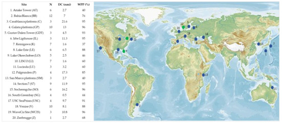
Figure 1.
Global map showing the 20 AERONET-OC sites considered in the study for the validation of PRISMA L2d data (blue dots represent coastal water sites, and green dots represent freshwater sites). n represents the number of PRISMA images acquired for each site, DC represents the distance from the coastline (expressed in nautical miles (nmi)), and WPP represents the average percentage of water pixels present in the scene acquired by PRISMA for each site.
Among the factors that may influence the quality of the data, the following were considered: estimated Chl-a concentration, measured AOD, absolute time lag between the acquisition of imagery and in situ spectra, view zenith angle, and sun zenith angle. In order to assess whether the variability in these factors influences the L2d products, the dataset was divided into two subsets according to the median value of each parameter. The median rather than the mean value was considered as to prevent the influence from outliers on the division into two subsets. The frequency distributions, mean and median values are shown in Figure 2. The DC parameter was also considered, where instead of the median value, the value of five nautical miles was selected, because around this value the adjacency effect could influence the accuracy of the satellite data, as demonstrated in [32,56].
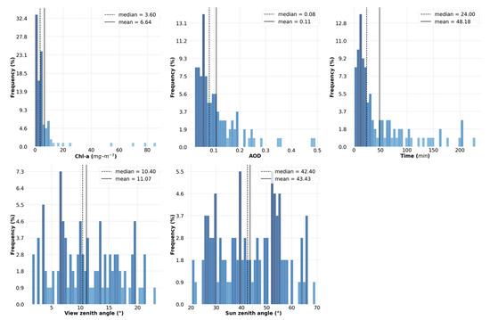
Figure 2.
Frequency distributions of estimated Chl-a concentration [32], measured AOD (550), absolute time lag between the acquisition of imagery and in situ spectra, view zenith angle, and sun zenith angle. The continuous vertical lines represent the mean value, while the dashed lines refer to the median value.
2.4. Match-Up Analysis
For the comparison with AERONET-OC data, the average of a 3 × 3 pixel matrix, centered around the in situ station (similarly to [32]), was extracted from the processed PRISMA data. Given the variability in the characteristics of aquatic sites, the closest in time to PRISMA acquisition were extracted for AERONET-OC. According to [32,57], a ±1 h time window was considered, with the exception of some cases where the time window was extended to ±4 h, as there were no AERONET-OC data available closer in time. Nevertheless, the vast majority of match-ups for this study (78 out of 109) occurred within 1 h and more than half (60 out of 109) were within 30 min (Figure 2). A qualitative comparison of PRISMA and in situ reflectance, at their original spectral resolutions, was performed in the range of 440–900 nm. For the quantitative analysis, a set of descriptive statistics was calculated to assess the consistency between PRISMA L2d and in situ data: the root mean square error (RMSE), the spectral angle (SA), the median symmetric accuracy (MdSA) (%), and symmetric signed percentage bias (Bias) (%) [58]. MdSA and Bias were used rather than the common coefficient of determination (R2), as the latter is not always ideal in ocean color studies, which are often limited by sample availability (in accordance with [59]). The SA was used to determine how similar the shape of PRISMA spectra is to in situ data. The metrics used for the analysis were computed as follows:
where is the in situ Rrs data, is the PRISMA-estimated Rrs data, n is the number of concurrent observations of the match-up, M is the median, and . In order to perform the statistical analysis, the PRISMA bands closest to the corresponding bands of the multispectral configuration of AERONET-OC were selected.
3. Results and Discussion
This section shows the results obtained from the comparison between PRISMA L2d products and in situ measurements.
3.1. Qualitative Assessment
Figure 3 shows the site-based qualitative comparisons of the mean spectra and their standard deviations associated with PRISMA L2d and AERONET-OC data. Overall, depending on the water conditions and related optical complexity, satellite and in situ spectra of each site vary greatly in terms of the shape of spectral signature and their magnitudes [8]. The typical shape of turbid water spectra can be recognized among the various sites, for example in the cases of the Ariake Tower site [60] (average Chl-a = 6.35 mg.m−3), the Bahia Blanca site [61] (average Chl-a = 4.26 mg.m−3) and the South Greenbay site [62] (average Chl-a = 78 mg.m−3), which show the peak of reflectance in the green region (around 570 nm) and a secondary maximum peak around 700 nm (associated with the presence of phytoplankton blooms). The typical shape of clear water spectra can be detected in the sites of the Casablanca platform (average Chl-a = 0.26 mg.m−3), Venise (average Chl-a = 0.73 mg.m−3), and the USC Seaprism (average Chl-a = 0.69 mg.m−3) where Rrs spectra are higher in the blue region and generally tend to decrease after about 505 nm. In the case of the Palgrunden site in Lake Vänern, the optical dominance of CDOM can be noted, given the significant absorption of light in the blue to the yellow region [63,64]. For the Lake Erie site, the reflectance trough around 620 nm in the PRISMA L2d spectra could be indicative of the absorption maximum associated with the presence of phycocyanin (PC), pigment related to the presence of cyanobacterial algal bloom [65,66]. Atypical is the spectrum of Lake Okeechobee, where marked absorption and reflectance peaks can be noted especially in the PRISMA Rrs spectra. The peculiarity of the spectral signature of this lake could be due to its characteristics: a shallow lake, rich in near-surface sediment concentrations, and characterized by seasonal cyanobacteria blooms [3,67]. The maximum Rrs values are observed for the Bahia Blanca and Zeebrugge sites, where the Rrs spectra of PRISMA L2d and AERONET-OC are in both cases around 0.025 sr−1, while in other cases the values are lower, such as at the Galata platform and LISCO sites, where the Rrs values of PRISMA L2d and AERONET-OC are at most 0.010 and 0.006 sr−1, respectively. The highest quality PRISMA L2d spectra can be found in the case of the Palgrunden site, where there is good agreement both in terms of magnitude and spectral shape, apart from the 440 nm reflectance which is overestimated in the L2d spectrum. In some cases, however, there is only good agreement in terms of the spectral shape (PRISMA’s overestimation of magnitude, see, e.g., Ariake Tower and South Greenbay spectra). Only in a few cases there is poor agreement between the data, such as for Casablanca and San Marco platforms. It is also possible to see in some cases (e.g., Irbe Lighthouse, Venise, Socheongcho and Gustav Dalen Tower sites) that PRISMA L2d overestimated Rrs in the blue region, as also observed in [37]. These uncertainties could be related to the fact that for the Casablanca platform, Irbe Lighthouse, Socheongcho and Gustav Dalen Tower sites, the WPP is about 90%: since the ASI model used for the atmospheric correction relies on aerosol properties in encountered in terrestrial regions, this could lead to uncertainties in the estimation of the AOD, which subsequently influences the final reflectance products; in particular, there is an overestimation of the PRISMA Rrs spectrum compared to that measured in situ. For the San Marco platform, Socheongcho and Venise sites, PRISMA Rrs spectra are higher than in situ measurements, which could be due to sun-glint effects: in particular, this gap in the Rrs spectra is evident in the NIR region where the water signature decreases towards zero, especially in very clear waters [68]. It is also worth noting the unrealistic spectral variability at some of the sites (e.g., Casablanca, Galata platform). Such unphysical variability points to the presence of image artefacts (e.g., straylight), particularly in the blue portion of the spectrum and across sites with lower-magnitude spectra (i.e., either blue or organic-rich waters). The various peaks and troughs shown in PRISMA spectra may be partially due to the effect of an insufficient atmospheric correction, also highlighted in [37].
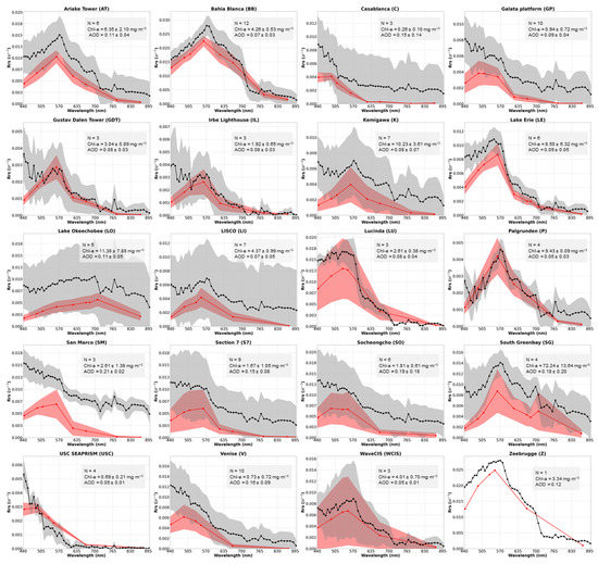
Figure 3.
Comparisons of mean PRISMA L2d and AERONET-OC Rrs data. The variability in the mean spectra of PRISMA L2d is displayed in dark curves with the shaded grey area representing one standard deviation. The mean and standard deviation of AERONET-OC are equivalently shown in red.
3.2. Quantitative Analysis
A more detailed single-band analysis was performed to gauge the quality of PRISMA L2d products across different spectral regions: the results of this analysis are shown in Figure 4. For each band, there was a different sample size (n), as AERONET-OC instruments have different spectral configurations [49]. In general, PRISMA L2d better agree with in situ spectra in the 490–709 nm bands compared to the NIR bands. From this analysis, however, it can be seen that PRISMA L2d does not present strong statistical agreement with the in situ data in the 443 nm band, and this could still be due to the fact that in the blue region, PRISMA L1 data may suffer from instrument artifacts or calibration issues [36,37]. Due to the poor agreement in the NIR region, the 779 and 865 nm bands were removed from the analysis. Overall, removing these two bands resulted in a change in the degree of statistical agreement between the data: SA changed from 17.5° to 15.3° and MdSA diminished from 82.1% to 66.7%.
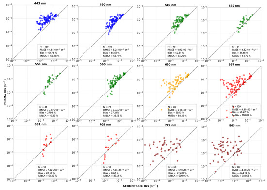
Figure 4.
Scatterplots between in situ and PRISMA L2d Rrs measurements, for each of the 12 bands considered (x-axis shows in situ data while the y-axis shows PRISMA L2d data). n represents the sample size. Scatterplots are shown in log-log scale and the dashed black line refers to the 1:1 line.
In Figure 5, the spectral residuals of the entire dataset are presented in order to highlight where there is less deviation between the satellite data and the in situ measurements: residuals are expressed in terms of Rrs difference (residuals = Rrs PRISMA L2d − Rrs AERONET-OC) [41]. Referring to the mean and median (continuous and dashed line, respectively), the residual values are slightly higher in the blue and in the red spectral regions (especially when examining the mean line). Furthermore, the graph shows that usually when there is disagreement in the match-ups, it is due to an overestimation of the PRISMA Rrs spectrum compared to the in situ measurement.
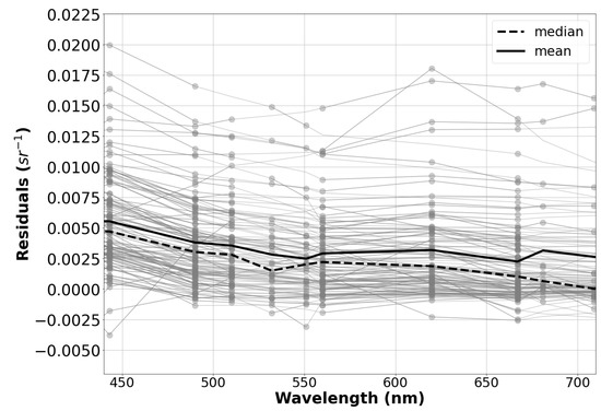
Figure 5.
Residuals (Rrs PRISMA L2d − Rrs AERONET-OC) obtained from the difference between PRISMA L2d and in situ measurements, in terms of Rrs (sr−1). The continuous line represents the mean, while the dashed line represents the median.
Figure 6 shows the specific statistical results for each image in the dataset, displaying MdSA (%), RMSE (sr−1), and SA (°) metrics. Following the observations in the qualitative analysis (Figure 3), the quantitative analysis shows a high degree of agreement, for example, for the Bahia Blanca site (which shows the lowest SA values), the Palgrunden site (noted in particular in terms of RMSE), and the Lake Erie site (low RMSE and MdSA values). It should be noted that in some cases, there are low SA values and higher MdSA values, which could be due to spectra that have similar shapes but differ in magnitude (usually overestimating the Rrs spectrum of PRISMA compared to AERONET-OC), as in the case of the Ariake Tower site. This could be caused by several factors, such as an inaccurate estimation of the AOD. The Casablanca and San Marco platforms show low RMSE values, probably due to the low values of their Rrs spectra, but show MdSA values greater than 200%. In particular, the weak agreement obtained for the Casablanca platform site could be its offshore location, more than 20 nautical miles from the coastline, where a more viable water-specific atmospheric correction with built-in “maritime” aerosol models maybe more suitable. In the following graphs, the bars represent the SA (expressed in degrees), and the color represents the season (summer: October–March in the Southern Hemisphere and April–September in the Northern Hemisphere; winter: October–March in the Northern Hemisphere and April–September in the Southern Hemisphere).
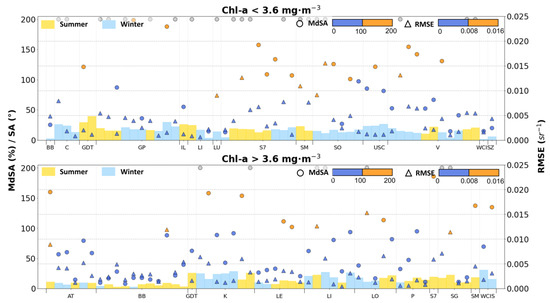
Figure 6.
Statistical analysis to assess the accuracy of the data through representation of three different metrics: MdSA (%) and SA (°) on the principal axis, RMSE (sr−1) on the secondary axis. The SA is represented by the bars in the graph. The grey dots refer to cases where the MdSA value is over 200%. In the x-axis are reported the 20 different sites (using the acronyms shown in Figure 1).
3.3. Dependency on Ancillary Data
As mentioned in Section 2.3, considering the median value (3.6 mg·m−3) of Chl-a concentration available in AERONET-OC, 54 of the 109 images were associated with clear water types and 55 with productive waters. A better degree of statistical agreement was found in meso-eutrophic waters (Figure 7): SA = 12.4°, RMSE = 0.002 sr−1, Bias = 40%, and MdSA = 46% (for the clear waters: SA = 16.8°, RMSE = 0.004, Bias = 70%, and MdSA = 85%). This may be due to the fact that there is a higher water-leaving signal, making it less sensitive to uncertainties in the atmospheric correction, in accordance with [37]. This confirms that the underwater light field may influence the accuracy of satellite data, especially in coastal waters that are characterized by a large variability in optically components, especially CDOM and TSM caused by bio-geochemical processes, meteo-marine forcing (wind, currents and tides), as well as run-off from land and river inflows [69].
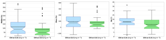
Figure 7.
Box plots referring to the Chl-a concentration (3.6 mg·m−3 represents the median value). The box plot in blue is representative of water types with clear water characteristics while the box plot in green is representative of phytoplankton-rich waters (i.e., with a Chl-a concentration >3.6 mg·m−3). The continuous line represents the median while the dashed line represents the mean.
In Figure 8, box plots for the parameters of AOD, view zenith angle, sun zenith angle and DC are displayed. For lower AOD values, there is a higher degree of statistical agreement (SA = 15.2°, RMSE = 0.001 sr−1, Bias = 12%, and MdSA = 33%). Since the contribution of the atmospheric path radiance in the VNIR spectrum accounts for up to 90% of the radiance measured by the sensor (e.g., [70]), especially for higher AOD concentrations, a greater portion of the radiance may be absorbed by aerosols and, thus, not be recorded by the sensor. This can lead to alterations in the magnitude of the spectral signatures obtained from satellite images. Regarding the statistical analysis of the view zenith angle, no major changes were noticed from a static viewpoint. Only a very slight variation occurred for view zenith < 10.4° (increase in the degree of statistical agreement: SA = 15.4°, RMSE = 0.003 sr−1, Bias = 51%, and MdSA = 64%); this could be due to the calibration and validation of the sensors (usually limited to targets observed near nadir), since as the view angle increases, the quality of the satellite products degrades (as mentioned in [71]). In the case of the sun zenith angle, for values greater than 42.4°, a greater statistical agreement was noted (SA = 15.5°, RMSE = 0.002 sr−1, Bias = 35%, and MdSA = 57%), as also reported in [72]. This could be due to the fact that for lower sun zenith values during the summer period, there is a greater probability of the presence of sun-glint. In fact, the variation is mainly in terms of magnitude since the SA value is unchanged. A little change in statistical agreement was also observed in the case of the parameter relating to the DC: a higher degree of statistical agreement was observed for sites at a distance of more than five nautical miles from the coastline (SA = 15.1°, RMSE = 0.002 sr−1, Bias = 34%, and MdSA = 65%). This is most likely due to the adjacency effect for sites closer to the coastline (as mentioned in [32,49]).
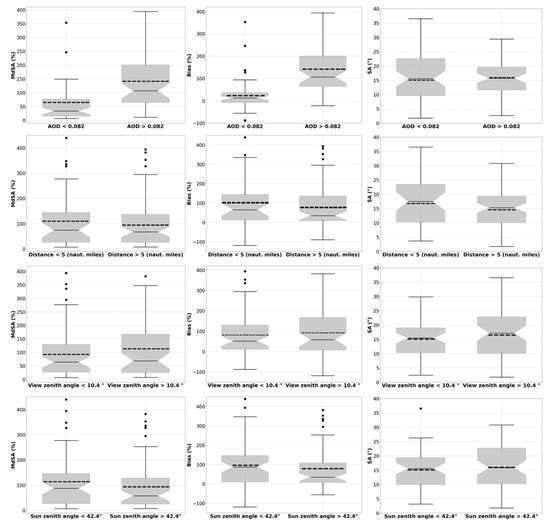
Figure 8.
Box plots referring to the AOD (0.082 represents the median value), view zenith angle (10.4° represents the median value), sun zenith angle (42.4° represents the median value) and Distance from the coastline (5 nautical miles represent a threshold value in accordance with [49]). The continuous line represents the median while the dashed line represents the mean.
4. Conclusions
This study reports an evaluation of PRISMA’s standard (L2d) reflectance products, atmospherically corrected through an automatic processor provided by the ASI. This effort considers a larger dataset than a study previously carried out at two aquatic sites (lake and coastal water) [37]. In this work, in situ data extracted from the AERONET-OC network were used as reference data for the evaluation of PRISMA L2d data. In total, 109 cloud-free PRISMA images acquired, synchronous with in situ data from July 2019 to July 2022 at 20 sites (17 coastal waters and 3 lakes), were analyzed. The results showed that the degree of accordance between PRISMA’s L2d products and AERONET-OC spectra depends on several factors, such as the trophic state of the water, atmospheric conditions, and observation and illumination geometry. For instance, it was observed that the statistical agreement slightly increased for higher Chl-a concentration and for lower AOD values. On the other hand, considering the imaging geometry conditions and coastline distances, slight variations in the statistical agreement were observed. It was also noted that at some sites, PRISMA L2d processing method retains the in situ spectral shape adequately but showed some additional peaks and troughs, which may be due to instrument artifacts, the presence of sun-glint, or uncertainties in estimating the atmospheric path radiance. For some spectra, the magnitude of the reflectance was overestimated. As the PRISMA atmospheric correction processor to generate L2d products was designed for terrestrial applications [43,44], it exploits the correlation between the reflectance in the SWIR region and the blue and red bands, affecting the AOD retrieval in scenes with a high percentage of water pixels. Hence, the uncertainties of the estimated reflectance for aquatic targets, particularly evident in the clear water sites, could also be present in coastal sites due to the presence of few land pixels in the scene [37]. A future study including the use of water-specific atmospheric correction algorithms (e.g., ACOLITE, [73]), more inland water sites, and the use of hyperspectral in situ datasets would be needed to identify optimal atmospheric correction processors [37]. For example, the testing of different water-specific atmospheric correction processors in the atmospheric correction intercomparison exercise (ACIX) [74,75], conducted by NASA and ESA in coordination with the validation group of the Committee on Earth Observation Satellites (CEOS), should provide relevant findings.
Author Contributions
Conceptualization, A.P., A.F., M.B. and C.G.; methodology, A.P., A.F., M.B., V.E.B., F.B., T.M.A.d.L., N.P. and C.G.; validation, A.P. and A.F.; formal analysis, A.P., A.F., M.B. and C.G.; investigation, A.P., A.F., M.B., F.B. and C.G.; resources, M.B., F.B., S.K. and C.G.; data curation, A.P., A.F. and T.M.A.d.L.; writing—original draft preparation, A.P., A.F., M.B., N.P. and C.G.; writing—review and editing, A.P., C.G., M.B., A.F., F.B., T.M.A.d.L., N.P., V.E.B., S.K. and M.G. All authors have read and agreed to the published version of the manuscript.
Funding
This work was supported by the Italian Space Agency with the PRISCAV Project (grant nr. 2019-5- HH.0) focusing on the CAL/VAL activities of the PRISMA hyperspectral sensor and with PANDA-WATER Project (Contract ASI N. 2022-15-U.0). The EU Horizon 2020 programme also co-founded the work through the PrimeWater Project (GA No. 870497). Nima Pahlevan was funded under NASA Ocean Biology and Biogeochemistry (OBB) program grant #80NSSC21K0499. Susanne Kratzer was funded under the Swedish National Space Agency infrastructure grant #2021-00050.
Data Availability Statement
The datasets generated during and/or analyzed during the current study are available from the corresponding author on reasonable request.
Acknowledgments
We are very grateful to the AERONET-OC Principal Investigators: J. Ishizaka, K. Arai, H. Loisel, P. Pratolongo, R. Frouin, M. Talone, F. Mélin, B. Bulgarelli, G. Zibordi, H. Higa, T. Moore, S. Ru-berg, M. Wang, S. Ahmed, A. Gilerson, T. Schroeder, Y.J. Park, B. Jones, M. Ragan, S. Ladner, and D. Van der Zande; the Joint Research Centre (JRC) of the European Commission; and the JAXA’s GCOM-C project. Data were sourced from Australia’s Integrated Marine Observing System (IMOS); IMOS is enabled by the National Collaborative Research Infrastructure Strategy (NCRIS). IMOS (NCRIS) and CSIRO are acknowledged for funding the Lucinda Jetty Coastal Observatory. We are very grateful to the anonymous reviewers for their detailed comments that significantly improved the manuscript.
Conflicts of Interest
The authors declare no conflict of interest.
References
- Bopp, L.; Boyd, P.; Donner, D.; Kiessling, W.; Martinetto, P.; Ojea, E.; Racault, M.; Rost, B.; Skern-Mauritzen, M.; Ghebrehiwet, M.; et al. Oceans and Coastal Ecosystems and Their Services. In Climate Change 2022: Impacts, Adaptation and Vulnerability; Contribution of Working Group II to the Sixth Assessment Report of the Intergovernmental Panel on Climate Change; Cambridge University Press: Cambridge, UK; New York, NY, USA, 2022; pp. 379–550. [Google Scholar] [CrossRef]
- Olmanson, L.G.; Brezonik, P.L.; Bauer, M.E. Airborne hyperspectral remote sensing to assess spatial distribution of water quality characteristics in large rivers: The Mississippi River and its tributaries in Minnesota. Remote Sens. Environ. 2013, 130, 254–265. [Google Scholar] [CrossRef]
- Pahlevan, N.; Smith, B.; Schalles, J.; Binding, C.; Cao, Z.; Ma, R.; Alikas, K.; Kangro, K.; Gurlin, D.; Hà, N.; et al. Seamless retrievals of chlorophyll-a from Sentinel-2 (MSI) and Sentinel-3 (OLCI) in inland and coastal waters: A machine-learning approach. Remote Sens. Environ. 2020, 240, 111604. [Google Scholar] [CrossRef]
- Vignolo, A.; Pochettino, A.; Cicerone, D. Water quality assessment using remote sensing techniques: Medrano Creek, Argentina. J. Environ. Manag. 2006, 81, 429–433. [Google Scholar] [CrossRef] [PubMed]
- Odermatt, D.; Gitelson, A.; Brando, V.E.; Schaepman, M. Review of constituent retrieval in optically deep and complex waters from satellite imagery. Remote Sens. Environ. 2012, 118, 116–126. [Google Scholar] [CrossRef]
- Tyler, A.N.; Hunter, P.D.; Spyrakos, E.; Groom, S.; Constantinescu, A.M.; Kitchen, J. Developments in Earth observation for the assessment and monitoring of inland, transitional, coastal and shelf-sea waters. Sci. Total Environ. 2016, 572, 1307–1321. [Google Scholar] [CrossRef]
- Stuart, M.B.; McGonigle, A.J.S.; Willmott, J.R. Hyperspectral Imaging in Environmental Monitoring: A Review of Recent Developments and Technological Advances in Compact Field Deployable Systems. Sensors 2019, 19, 3071. [Google Scholar] [CrossRef]
- Giardino, C.; Brando, V.E.; Gege, P.; Pinnel, N.; Hochberg, E.; Knaeps, E.; Reusen, I.; Doerffer, R.; Bresciani, M.; Braga, F.; et al. Imaging Spectrometry of Inland and Coastal Waters: State of the Art, Achievements and Perspectives. Surv. Geophys. 2019, 40, 401–429. [Google Scholar] [CrossRef]
- Brando, V.E.; Dekker, A.G. Satellite hyperspectral remote sensing for estimating estuarine and coastal water quality. IEEE Trans. Geosci. Remote Sens. 2003, 41, 1378–1387. [Google Scholar] [CrossRef]
- Zhu, W.; Tian, Y.Q.; Yu, Q.; Becker, B.L. Using Hyperion imagery to monitor the spatial and temporal distribution of colored dissolved organic matter in estuarine and coastal regions. Remote Sens. Environ. 2013, 134, 342–354. [Google Scholar] [CrossRef]
- Cho, H.J.; Ogashawara, I.; Mishra, D.; White, J.; Kamerosky, A.; Morris, L.; Clarke, C.; Simpson, A.; Banisakher, D. Evaluating Hyperspectral Imager for the Coastal Ocean (HICO) data for seagrass mapping in Indian River Lagoon, FL. GIScience Remote Sens. 2014, 51, 120–138. [Google Scholar] [CrossRef]
- O’Shea, R.E.; Pahlevan, N.; Smith, B.; Bresciani, M.; Egerton, T.; Giardino, C.; Li, L.; Moore, T.; Ruiz-Verdu, A.; Ruberg, S.; et al. Advancing cyanobacteria biomass estimation from hyperspectral observations: Demonstrations with HICO and PRISMA imagery. Remote Sens. Environ. 2021, 266, 112693. [Google Scholar] [CrossRef]
- Van Mol, B.; Ruddick, K. The Compact High Resolution Imaging Spectrometer (CHRIS): The future of hyperspectral satellite sensors. Imagery of Oostende coastal and inland waters. In Proceedings of the Airborne Imaging Spectroscopy Workshop, Brugge, Belgium, 8 October 2004. [Google Scholar]
- Wang, Q.; Zhang, Z.; Hao, Z.; Liu, B.; Xiong, J. Optical Classification of Coastal Water Body in China using Hyperspectral Imagery CHRIS/PROBA. In Proceedings of the IOP Conference Series: Earth and Environmental Science, Surakarta, Indonesia, 11–13 December 2020. [Google Scholar]
- Coppo, P.; Brandani, F.; Faraci, M.; Sarti, F.; Cosi, M. Leonardo Spaceborne Infrared Payloads for Earth Observation: SLSTRs for Copernicus Sentinel 3 and PRISMA Hyperspectral Camera for PRISMA Satellite. Appl. Opt. 2020, 59, 6888–6901. [Google Scholar] [CrossRef] [PubMed]
- Lopinto, E.; Ananasso, C. The Prisma hyperspectral mission. In Proceedings of the 33rd EARSeL Symposium, Towards Horizon, Matera, Italy, 3–7 June 2013; pp. 3–7. [Google Scholar]
- Cogliati, S.; Sarti, F.; Chiarantini, L.; Cosi, M.; Lorusso, R.; Lopinto, E.; Miglietta, F.; Genesio, L.; Guanter, L.; Damm, A.; et al. The PRISMA imaging spectroscopy mission: Overview and first performance analysis. Remote Sens. Environ. 2021, 262, 112499. [Google Scholar] [CrossRef]
- Bresciani, M.; Giardino, C.; Fabbretto, A.; Pellegrino, A.; Mangano, S.; Free, G.; Pinardi, M. Application of New Hyperspectral Sensors in the Remote Sensing of Aquatic Ecosystem Health: Exploiting PRISMA and DESIS for Four Italian Lakes. Resources 2022, 11, 8. [Google Scholar] [CrossRef]
- Niroumand-Jadidi, M.; Bovolo, F.; Bruzzone, L. Water quality retrieval from PRISMA hyperspectral images: First experience in a turbid lake and comparison with sentinel-2. Remote Sens. 2020, 12, 3984. [Google Scholar] [CrossRef]
- Borfecchia, F.; Micheli, C.; De Cecco, L.; Sannino, G.; Struglia, M.V.; Di Sarra, A.G.; Gomez, C.; Mattiazzo, G. Satellite multi/hyper spectral HR sensors for mapping the Posidonia oceanica in south mediterranean islands. Sustainability 2021, 13, 13715. [Google Scholar] [CrossRef]
- Lima, T.M.A.D.; Giardino, C.; Bresciani, M.; Barbosa, C.C.F.; Fabbretto, A.; Pellegrino, A.; Begliomini, F.N. Assessment of Estimated Phycocyanin and Chlorophyll-a Concentration from PRISMA and OLCI in Brazilian Inland Waters: A Comparison between Semi-Analytical and Machine Learning Algorithms. Remote Sens. 2023, 15, 1299. [Google Scholar] [CrossRef]
- Taggio, N.; Aiello, A.; Ceriola, G.; Kremezi, M.; Kristollari, V.; Kolokoussis, P.; Karathanassi, V.; Barbone, E. A Combination of machine learning algorithms for marine plastic litter detection exploiting hyperspectral PRISMA data. Remote Sens. 2022, 14, 3606. [Google Scholar] [CrossRef]
- Giardino, C.; Brando, V.E.; Dekker, A.G.; Strömbeck, N.; Candiani, G. Assessment of water quality in Lake Garda (Italy) using Hyperion. Remote Sens. Environ. 2007, 109, 183–195. [Google Scholar] [CrossRef]
- Braga, F.; Giardino, C.; Bassani, C.; Matta, E.; Candiani, G.; Strömbeck, N.; Adamo, M.; Bresciani, M. Assessing water quality in the northern Adriatic Sea from HICO™ data. Remote Sens. Lett. 2013, 4, 1028–1037. [Google Scholar] [CrossRef]
- Pinardi, M.; Fenocchi, A.; Giardino, C.; Sibilla, S.; Bartoli, M.; Bresciani, M. Assessing Potential Algal Blooms in a Shallow Fluvial Lake by Combining Hydrodynamic Modelling and Remote-Sensed Images. Water 2015, 7, 1921–1942. [Google Scholar] [CrossRef]
- Wang, M. Atmospheric Correction for Remotely-Sensed Ocean-Colour Products. Reports and Monographs of the International Ocean-Colour Coordinating Group (IOCCG). 2010. Available online: http://dx.doi.org/10.25607/OBP-101 (accessed on 26 February 2023). [CrossRef]
- Gordon, H.R.; Castaño, D.J. Coastal Zone Color Scanner atmospheric correction algorithm: Multiple scattering effects. Appl. Opt. 1987, 26, 2111–2122. [Google Scholar] [CrossRef] [PubMed]
- Sterckx, S.; Brown, I.; Kääb, A.; Krol, M.; Morrow, R.; Veefkind, P.; Boersma, K.F.; De Mazière, M.; Fox, N.; Thorne, P. Towards a European Cal/Val service for earth observation. Int. J. Remote Sens. 2020, 41, 4496–4511. [Google Scholar] [CrossRef]
- Concha, J.A.; Bracaglia, M.; Brando, V.E. Assessing the influence of different validation protocols on Ocean Colour match-up analyses. Remote Sens. Environ. 2021, 259, 112415. [Google Scholar] [CrossRef]
- Justice, C.; Belward, A.; Morisette, J.; Lewis, P.; Privette, J.; Baret, F. Developments in the’validation’of satellite sensor products for the study of the land surface. Int. J. Remote Sens. 2000, 21, 3383–3390. [Google Scholar] [CrossRef]
- Bailey, S.W.; Werdell, P.J. A multi-sensor approach for the on-orbit validation of ocean color satellite data products. Remote Sens. Environ. 2006, 102, 12–23. [Google Scholar] [CrossRef]
- Zibordi, G.; Mélin, F.; Berthon, J.-F.; Holben, B.; Slutsker, I.; Giles, D.; D’Alimonte, D.; Vandemark, D.; Feng, H.; Schuster, G.; et al. AERONET-OC: A network for the validation of ocean color primary products. J. Atmos. Ocean. Technol. 2009, 26, 1634–1651. [Google Scholar] [CrossRef]
- Pahlevan, N.; Balasubramanian, S.V.; Sarkar, S.; Franz, B.A. Toward Long-Term Aquatic Science Products from Heritage Landsat Missions. Remote Sens. 2018, 10, 1337. [Google Scholar] [CrossRef]
- Vanhellemont, Q. Adaptation of the dark spectrum fitting atmospheric correction for aquatic applications of the Landsat and Sentinel-2 archives. Remote Sens. Environ. 2019, 225, 175–192. [Google Scholar] [CrossRef]
- Ilori, C.O.; Pahlevan, N.; Knudby, A. Analyzing Performances of Different Atmospheric Correction Techniques for Landsat 8: Application for Coastal Remote Sensing. Remote Sens. 2019, 11, 469. [Google Scholar] [CrossRef]
- Giardino, C.; Bresciani, M.; Braga, F.; Fabbretto, A.; Ghirardi, N.; Pepe, M.; Gianinetto, M.; Colombo, R.; Cogliati, S.; Ghebrehiwot, S.; et al. First Evaluation of PRISMA Level 1 Data for Water Applications. Sensors 2020, 20, 4553. [Google Scholar] [CrossRef] [PubMed]
- Braga, F.; Fabbretto, A.; Vanhellemont, Q.; Bresciani, M.; Giardino, C.; Scarpa, G.M.; Manfè, G.; Concha, J.A.; Brando, V.E. Assessment of PRISMA water reflectance using autonomous hyperspectral radiometry. ISPRS J. Photogramm. Remote Sens. 2022, 192, 99–114. [Google Scholar] [CrossRef]
- Jamet, C.; Loisel, H.; Kuchinke, C.P.; Ruddick, K.; Zibordi, G.; Feng, H. Comparison of three SeaWiFS atmospheric correction algorithms for turbid waters using AERONET-OC measurements. Remote Sens. Environ. 2011, 115, 1955–1965. [Google Scholar] [CrossRef]
- Hlaing, S.; Gilerson, A.; Harmel, T.; Tonizzo, A.; Weidemann, A.; Arnone, R.; Ahmed, S. Assessment of a bidirectional reflectance distribution correction of above-water and satellite water-leaving radiance in coastal waters. Appl. Opt. 2012, 51, 220–237. [Google Scholar] [CrossRef] [PubMed]
- Mélin, F.; Clerici, M.; Zibordi, G.; Holben, B.N.; Smirnov, A. Validation of SeaWiFS and MODIS aerosol products with globally distributed AERONET data. Remote Sens. Environ. 2010, 114, 230–250. [Google Scholar] [CrossRef]
- Mélin, F. Validation of ocean color remote sensing reflectance data: Analysis of results at European coastal sites. Remote Sens. Environ. 2022, 280, 113153. [Google Scholar] [CrossRef]
- Guarini, R.; Loizzo, R.; Longo, F.; Mari, S.; Scopa, T.; Varacalli, G. Overview of the prisma space and ground segment and its hyperspectral products. In Proceedings of the 2017 IEEE International Geoscience and Remote Sensing Symposium (IGARSS), Fort Worth, TX, USA, 23–28 July 2017; pp. 431–434. [Google Scholar] [CrossRef]
- ASI—Italian Space Agency, 2021. PRISMA Algorithm Theoretical Basis Document (ATBD), Issue 1, Date 14/12/2021. Available online: http://prisma.asi.it/missionselect/docs.php (accessed on 7 May 2022).
- Ouaidrari, H.; Vermote, E.F. Operational Atmospheric Correction of Landsat TM Data. Remote Sens. Environ. 1999, 70, 4–15. [Google Scholar] [CrossRef]
- Warren, M.A.; Simis, S.G.; Martinez-Vicente, V.; Poser, K.; Bresciani, M.; Alikas, K.; Spyrakos, E.; Giardino, C.; Ansper, A. Assessment of atmospheric correction algorithms for the Sentinel-2A MultiSpectral Imager over coastal and inland waters. Remote Sens. Environ. 2019, 225, 267–289. [Google Scholar] [CrossRef]
- Valente, A.; Sathyendranath, S.; Brotas, V.; Groom, S.; Grant, M.; Taberner, M.; Antoine, D.; Arnone, R.; Balch, W.M.; Barker, K.; et al. A compilation of global bio-optical in situ data for ocean-colour satellite applications–version two. Earth Syst. Sci. Data 2019, 11, 1037–1068. [Google Scholar] [CrossRef]
- Zibordi, G.; D’Alimonte, D.; Kajiyama, T. Automated Quality Control of AERONET-OC L WN Data. J. Atmos. Ocean. Technol. 2022, 39, 1961–1972. [Google Scholar] [CrossRef]
- Cazzaniga, I.; Zibordi, G. AERONET-OC L WN Uncertainties: Revisited. J. Atmos. Ocean. Technol. 2023, 40, 411–425. [Google Scholar] [CrossRef]
- Zibordi, G.; Holben, B.N.; Talone, M.; D’Alimonte, D.; Slutsker, I.; Giles, D.M.; Sorokin, M.G. Advances in the ocean color component of the aerosol robotic network (AERONET-OC). J. Atmos. Ocean. 2021, 38, 725–746. [Google Scholar] [CrossRef]
- Zibordi, G.; Mélin, F.; Berthon, J.F. Comparison of SeaWiFS, MODIS and MERIS radiometric products at a coastal site. Geophys. Res. Lett. 2006, 33, 1–4. [Google Scholar] [CrossRef]
- Pahlevan, N.; Sarkar, S.; Franz, B.A.; Balasubramanian, S.V.; He, J. Sentinel-2 MultiSpectral Instrument (MSI) data processing for aquatic science applications: Demonstrations and validations. Remote Sens. Environ. 2017, 201, 47–56. [Google Scholar] [CrossRef]
- Fan, Y.; Li, W.; Gatebe, C.K.; Jamet, C.; Zibordi, G.; Schroeder, T.; Stamnes, K. Atmospheric correction over coastal waters using multilayer neural networks. Remote Sens. Environ. 2017, 199, 218–240. [Google Scholar] [CrossRef]
- Tan, J.; Frouin, R.; Ramon, D.; Steinmetz, F. On the adequacy of representing water reflectance by semi-analytical models in ocean color remote sensing. Remote Sens. 2019, 11, 2820. [Google Scholar] [CrossRef]
- Thuillier, G.; Hersé, M.; Labs, D.; Foujols, T.; Peetermans, W.; Gillotay, D.; Simon, P.C.; Mandel, H. The solar spectral irradiance from 200 to 2400 nm as measured by the SOLSPEC spectrometer from the ATLAS and EURECA missions. Sol. Phys. 2003, 214, 1–22. [Google Scholar] [CrossRef]
- Giles, D.M.; Sinyuk, A.; Sorokin, M.G.; Schafer, J.S.; Smirnov, A.; Slutsker, I.; Eck, T.F.; Holben, B.N.; Lewis, J.R.; Campbell, J.R.; et al. Advancements in the Aerosol Robotic Network (AERONET) Version 3 database—Algoritmo di controllo della qualità quasi in tempo reale automatizzato con screening delle nuvole migliorato per le misurazioni della profondità ottica dell’aerosol (AOD) del fotometro solare. Atmos. Mis. Tech. 2019, 12, 169–209. [Google Scholar] [CrossRef]
- Bulgarelli, B.; Zibordi, G. On the detectability of adjacency effects in ocean color remote sensing of mid-latitude coastal en-vironments by SeaWiFS, MODIS-A, MERIS, OLCI, OLI and MSI. Remote Sens. Environ. 2018, 209, 423–438. [Google Scholar] [CrossRef]
- Van der Zande, D.; Vanhellemont, Q.; De Keukelaere, L.; Knaeps, E.; Ruddick, K. Validation of Landsat-8/OLI for ocean colour applications with AERONET-OC sites in Belgian coastal waters. In Proceedings of the Ocean Optics Conference, Victoria, BC, Canada, 23–28 October 2016. [Google Scholar]
- Morley, S.K.; Brito, T.V.; Welling, D.T. Measures of model performance based on the log accuracy ratio. Space Weather 2018, 16, 69–88. [Google Scholar] [CrossRef]
- Seegers, B.N.; Stumpf, R.P.; Schaeffer, B.A.; Loftin, K.A.; Werdell, P.J. Performance metrics for the assessment of satellite data products: An ocean color case study. Opt. Express 2018, 26, 7404–7422. [Google Scholar] [CrossRef] [PubMed]
- Jia, R.; Lei, H.; Hino, T.; Arulrajah, A. Environmental changes in Ariake Sea of Japan and their relationships with Isahaya Bay reclamation. Mar. Pollut. Bull. 2018, 135, 832–844. [Google Scholar] [CrossRef]
- Guinder, V.A.; Popovich, C.A.; Molinero, J.C.; Marcovecchio, J. Phytoplankton summer bloom dynamics in the Bahía Blanca Estuary in relation to changing environmental conditions. Cont. Shelf Res. 2013, 52, 150–158. [Google Scholar] [CrossRef]
- Qualls, T.; Harris, H.J.; Harris, V. The state of the bay: The condition of the bay of Green Bay/Lake Michigan. In NOAA Repository; 2013. Available online: https://repository.library.noaa.gov/view/noaa/34653/noaa_34653_DS1.pdf (accessed on 26 February 2023).
- Eleveld, M.A.; Ruescas, A.B.; Hommersom, A.; Moore, T.S.; Peters, S.W.M.; Brockmann, C. An Optical Classification Tool for Global Lake Waters. Remote Sens. 2017, 9, 420. [Google Scholar] [CrossRef]
- Philipson, P.; Kratzer, S.; Ben Mustapha, S.; Strömbeck, N.; Stelzer, K. Satellite-based water quality monitoring in Lake Vänern, Sweden. Int. J. Remote Sens. 2016, 37, 3938–3960. [Google Scholar] [CrossRef]
- Ho, J.C.; Michalak, A.M. Challenges in tracking harmful algal blooms: A synthesis of evidence from Lake Erie. J. Great Lakes Res. 2015, 41, 317–325. [Google Scholar] [CrossRef]
- Ogashawara, I. Determination of Phycocyanin from Space—A Bibliometric Analysis. Remote Sens. 2020, 12, 567. [Google Scholar] [CrossRef]
- Song, W.; Pang, Y. Research on narrow and generalized water environment carrying capacity, economic benefit of Lake Okeechobee, USA. Ecol. Eng. 2021, 173, 106420. [Google Scholar] [CrossRef]
- Cui, A.; Zhang, J.; Ma, Y.; Zhang, X. A Noise De-Correlation Based Sun Glint Correction Method and Its Effect on Shallow Bathymetry Inversion. Remote Sens. 2022, 14, 5981. [Google Scholar] [CrossRef]
- Mélin, F.; Zibordi, G.; Berthon, J.F. Assessment of satellite ocean color products at a coastal site. Remote Sens. Environ. 2007, 110, 192–215. [Google Scholar] [CrossRef]
- Gordon, H.R. Removal of atmospheric effects from satellite imagery of the oceans. Appl. Opt. 1978, 17, 1631–1636. [Google Scholar] [CrossRef] [PubMed]
- Barnes, B.B.; Hu, C. Dependence of satellite ocean color data products on viewing angles: A comparison between SeaWiFS, MODIS, and VIIRS. Remote Sens. Environ. 2016, 175, 120–129. [Google Scholar] [CrossRef]
- Mustard, J.F.; Staid, M.I.; Fripp, W.J. A semianalytical approach to the calibration of AVIRIS data to reflectance over water: Application in a temperate estuary. Remote Sens. Environ. 2001, 75, 335–349. [Google Scholar] [CrossRef]
- Vanhellemont, Q.; Ruddick, K. Atmospheric correction of metre-scale optical satellite data for inland and coastal water applications. Remote Sens. Environ. 2018, 216, 586–597. [Google Scholar] [CrossRef]
- Doxani, G.; Vermote, E.F.; Roger, J.-C.; Skakun, S.; Gascon, F.; Collison, A.; De Keukelaere, L.; Desjardins, C.; Frantz, D.; Hagolle, O.; et al. Atmospheric Correction Inter-comparison eXercise, ACIX-II Land: An assessment of atmospheric correction processors for Landsat 8 and Sentinel-2 over land. Remote Sens. Environ. 2023, 285, 113412. [Google Scholar] [CrossRef]
- Pahlevan, N.; Mangin, A.; Balasubramanian, S.V.; Smith, B.; Alikas, K.; Arai, K.; Barbosa, C.; Bélanger, S.; Binding, C.; Bresciani, M.; et al. ACIX-Aqua: A global assessment of atmospheric correction methods for Landsat-8 and Sentinel-2 over lakes, rivers, and coastal waters. Remote Sens. Environ. 2021, 258, 112366. [Google Scholar] [CrossRef]
Disclaimer/Publisher’s Note: The statements, opinions and data contained in all publications are solely those of the individual author(s) and contributor(s) and not of MDPI and/or the editor(s). MDPI and/or the editor(s) disclaim responsibility for any injury to people or property resulting from any ideas, methods, instructions or products referred to in the content. |
© 2023 by the authors. Licensee MDPI, Basel, Switzerland. This article is an open access article distributed under the terms and conditions of the Creative Commons Attribution (CC BY) license (https://creativecommons.org/licenses/by/4.0/).