Article

Dual-Level Contextual Attention Generative Adversarial Network for Reconstructing SAR Wind Speeds in Tropical Cyclones

1
School of Oceanography, Shanghai Jiao Tong University, Shanghai 200030, China
2
State Key Laboratory of Satellite Ocean Environment Dynamics, Second Institute of Oceanography, Ministry of Natural Resources, Hangzhou 310012, China
3
Southern Marine Science and Engineering Guangdong Laboratory (Zhuhai), Zhuhai 519082, China
4
National Marine Environmental Forecasting Center, Beijing 100081, China
5
Zhejiang Climate Centre, Hangzhou 310017, China
*
Author to whom correspondence should be addressed.
These authors contributed equally to this work.
Remote Sens. 2023, 15(9), 2454; https://doi.org/10.3390/rs15092454
Submission received: 16 April 2023 / Revised: 2 May 2023 / Accepted: 4 May 2023 / Published: 6 May 2023
(This article belongs to the Section Ocean Remote Sensing)

Abstract

:
Synthetic Aperture Radar (SAR) imagery plays an important role in observing tropical cyclones (TCs). However, the C-band attenuation caused by rain bands and the problem of signal saturation at high wind speeds make it impossible to retrieve the fine structure of TCs effectively. In this paper, a dual-level contextual attention generative adversarial network (DeCA-GAN) is tailored for reconstructing SAR wind speeds in TCs. The DeCA-GAN follows an encoder–neck–decoder architecture, which works well for high wind speeds and the reconstruction of a large range of low-quality data. A dual-level encoder comprising a convolutional neural network and a self-attention mechanism is designed to extract the local and global features of the TC structure. After feature fusion, the neck explores the contextual features to form a reconstructed outline and up-samples the features in the decoder to obtain the reconstructed results. The proposed deep learning model has been trained and validated using the European Centre for Medium-Range Weather Forecasts (ECMWF) atmospheric model product and can be directly used to improve the data quality of SAR wind speeds. Wind speeds are reconstructed well in regions of low-quality SAR data. The root mean square error of the model output and ECMWF in these regions is halved in comparison with the existing SAR wind speed product for the test set. The results indicate that deep learning methods are effective for reconstructing SAR wind speeds.

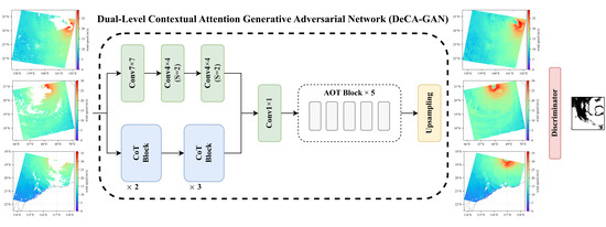
Graphical Abstract

1. Introduction

Tropical cyclones (TCs) are severe weather phenomena that occur over tropical oceans and are characterized by strong winds, heavy rain, and storm surges [1]. TCs are one of the most destructive natural disasters, causing significant damage to infrastructure and property and loss of life [2]. With continued global warming and socioeconomic development, TCs are becoming increasingly harmful, and accurately determining TC intensity and wind speed structure is crucial for timely preparation and reducing the impact of these disasters [3].
Synthetic Aperture Radar (SAR) is an active microwave sensor that estimates the sea surface wind field by measuring the intensity of radar echoes, known as the normalized radar cross-section (NRCS) [4]. SAR sensors, such as Sentinel-1A/B and Radarsat-2, have high-resolution imaging capabilities and can acquire multi-polarization data, which can improve the accuracy of TC forecasting [5,6]. With the advent of high-quality SAR images, various algorithms have emerged to retrieve wind fields. The use of geophysical model functions such as CMOD has been effective in retrieving wind speed from the NRCS of vertical–vertical (VV) and horizontal–horizontal (HH) polarized images. The Sentinel-1 wind speed product is based on the algorithm COMD-IFR2 developed by Institut Français de Recherche pour l’Exploitation de la Mer, with model inputs of NRCS values, incidence angles, track angles, a priori wind, and ice information [7]. However, for extreme cases such as TCs, a saturation phenomenon occurs, leading to a reduced accuracy in wind speed retrieval [8]. The use of cross-polarization SAR images (VH/HV) has been shown to solve the problem of signal saturation under strong winds [9,10]. In recent years, several algorithms have utilized SAR images to retrieve TC wind speeds, including the C-2PO model [11,12] and the advanced C-3PO model [13]. SAR images have also been used extensively to study the structures of TCs, such as symmetric double-eye structures, the radii of maximum wind speed, and the orientation of wind or waves within the storm [14,15,16]. However, accurately inverting the structure of TCs remains challenging due to C-band attenuation caused by rainfall and the problem of signal saturation at high wind speeds [15,17,18]. To the best of our knowledge, the progress of research on SAR wind speed reconstruction in TCs is still relatively limited.
Deep learning algorithms have shown great potential in processing SAR images of TCs to retrieve wind speed and analyze the structure of the storms. Boussioux et al. [19] used a multi-modal deep learning (DL) framework to combine multi-source data for hurricane forecasting. A DL method based on topological patterns was used with the high-resolution data of Sentinel-1 to improve the accuracy of TC intensity detection [20]. Progress has been made in exploring SAR wind speeds using DL, including deploying neural networks to invert sea surface wind speed from SAR and designing CNNs to extract SAR features to estimate TC intensity [21,22,23,24]. Using DL to construct forecast models based on Sentinel-1 and Sentinel-2 images has also shown good capability for offshore wind speed estimation [25]. These studies illustrate the great potential of DL in SAR wind speed processing. However, rain bands can cause C-band signal attenuation and extreme wind speeds can result in signal saturation, producing low-quality data and making it difficult for SAR to invert the TC structure accurately. Therefore, it is urgent to generate high accuracy wind speed data using DL to improve the low-quality SAR wind speed data and reconstruct the complete TC structure. However, due to the difficulty of leveraging the benefits of piece-wise linear units in the generative context, adopting only a CNN could cause problems for generative tasks such as SAR wind speed reconstruction. This situation has changed with the emergence of generative adversarial networks (GANs) [26], which correspond to a minimax two-player game in which a GAN framework with two networks, named the generator and the discriminator, are trained simultaneously. Furthermore, the ingenious approximation of some unsolvable loss functions by adversarial learning can promote the application of DL in generating tasks.
In order to fully exploit the ability of SAR to observe wind speed, especially during TCs, we propose a DL model for improving the low-quality data in SAR to reconstruct the TC structure directly. The reconstruction only targets the data in the low-quality region, retaining the original SAR high-precision wind speeds. In this way, the reconstructed results are based on real observations with a high resolution. This paper proposes a dual-level contextual attention GAN (DeCA-GAN) for reconstructing SAR wind speeds. A dual-level encoder is designed to help the model learn local and global TC features simultaneously. The neck part is designed to adaptively process the features extracted by the encoder and feed them to the decoder. The final result is generated under the guidance of the discriminator. The main contributions of this paper are as follows:
  • We propose a GAN-based deep learning model for directly enhancing the quality of SAR wind speeds and reconstructing the structure of TCs. The results are based on SAR observations and are close to reality, and thus can be used for TC intensity estimation, TC structure analysis, and forecast accuracy improvement.
  • The proposed model performs better than state-of-the-art models, especially for a large range of low-quality data and in high wind speed reconstruction. We also conduct ablation experiments to verify the components’ effectiveness in the proposed model.
  • The model is validated on ECMWF and SMAP, and the reconstructed results can be obtained in a few seconds using a single GPU. Compared to ECMWF, the reconstructed results achieve a relative reduction of 50% in the root mean square error (RMSE).
The rest of this paper is structured as follows: Section 2 presents our framework for SAR wind speed reconstruction in detail. In Section 3, we introduce the Sentinel-1 SAR TC images and present the experimental parameters and the results of reconstructed SAR wind speeds. We also conduct ablation experiments and visualize the feature maps inside the DeCA-GAN model to demonstrate its effectiveness. The discussions and conclusions are presented in Section 4 and Section 5, respectively.

2. Method

2.1. Architecture

This paper combines the advantages of dilated convolution [27] and the attention mechanism [28,29] and proposes a novel network for reconstructing SAR wind speeds in TCs. The overall encoder–neck–decoder framework of the proposed model DeCA-GAN is shown in Figure 1. The encoder includes two branches, which can simultaneously obtain local and global level semantic features from SAR wind speeds. After fusing the dual-level features, the new feature maps are sent to the neck part after dimensionality reduction. In this way, our model can learn TC structure and gain valuable features from both neighbor and distant pixels in the image. The neck of the model includes five AOT blocks based on work by Zeng et al. [30], which have various receptive fields on feature maps with the help of special dilated convolution designs. The outputs of the neck contain abstract and high-level semantic features. After two up-sampling operations, the model will generate a reconstructed TC image. The effect of the reconstruction will be further enhanced under the supervision of the discriminator.

2.2. Encoder Based on Dual-Level Learning

The encoder of the DeCA-GAN has two pathways responsible for local and global feature extraction, respectively. Suppose the encoder takes an image with a resolution of 160 × 160 × 1 (height, width, and channel, respectively). The first path of the encoder passes through a 7 × 7 convolutional layer and two 3 × 3 convolutional layers with stride 2. After that, the image shape will become 40 × 40 × 256. In particular, each convolutional layer in the first path is followed by an ECA module [31], as described in Section 2.2.2. This pathway mainly processes the local-level relationships in images. In addition, the DeCA-GAN employs another pathway to extract global relationships between pixels in images by using the contextual transformer (CoT) attention mechanism [29] (see Section 2.2.1). As shown in Figure 2, the CoT block first passes input x through a 1 × 1 convolutional layer, followed by a CoT module. The next 1 × 1 convolutional layer expands the channel dimensions, and this layer down-samples the size of the feature maps. Then, x′ can be obtained via an ECA block and added to skip connection branch y to get output x″. Specifically, the CoT block repeats several times in the DeCA-GAN encoder, but only the first repetition executes the down-sample and expansion operations. After concatenating the feature maps of two pathways, the DeCA-GAN encoder employs a 1 × 1 convolutional layer to reduce dimensionality. In this paper, we attempt two additional strategies to determine the best method to fuse two-level feature maps: the first uses two consecutive 1 × 1 convolutional layers in the experiment, first expanding the number of channels and then decreasing them, and the second uses two consecutive 1 × 1 convolutional layers, one of which is used to change the channel dimension. However, the effect of the above two methods is not as good as the single 1 × 1 convolution used in this paper. Moreover, the output of the encoder is 160 × 160 × 256.

2.2.1. CoT Block

In computer vision tasks, a CNN is usually the preferred method. Convolutional layers can obtain higher-level semantic features in the image, giving the model better capabilities. Moreover, because the convolution is of a locally connected layer, its computational load is also small. However, similar to human vision, there is a contextual relationship between objects in an image. For example, it is reasonable for a cup to be on a table and not a train. The local convolution cannot learn the global context of an image well. Even if dilated convolution can be used to increase the receptive field [32], convolution still finds difficulty in exploring the connection between distant contexts, which plays a vital role in visual tasks [33,34,35]. Vaswani et al. [28] proposed an outstanding framework transformer, which possesses the self-attention mechanism to help models learn the more valuable spatial features of the entire image. This new technique has been widely adopted in natural language processing (NLP) fields [36,37,38]. In the self-attention mechanism, the data matrix is copied as k, q, and v, denoted as key, query, and value, respectively. The whole process of self-attention is formulated as follows:
Attention ( q , k , v ) = softmax ( q k T d i m ) v ,
where d i m is the length of a token (or a single word) in NLP. This operation allows q to calculate the similarity with k by performing matrix multiplication and paying more attention to corresponding high-similarity parts in v. As shown in Figure 3, we obtain a q that is more similar to k 1 , followed by k 2 and k 3 . The weight, w, denoted as an attention map, is actually the corresponding similarity to q and k (in the dashed box). Specifically, the more similar q and k are, the larger w will be, which means w 1 > w 2 > w 3 .
Inspired by this design, many CV works circumvent the above-mentioned CNN limits by using transformer structures such as ViT [39], DETR [40], and Swin [41]. Some other works directly replace the CNN with a self-attention module [42,43] in ResNet [44]. However, those architectures only consider relationships between q and k independently without exploring valuable features among neighbor keys. CoT [29] is designed to capture static and dynamic contexts simultaneously, with a better effect than vanilla self attention and derivatives of ResNet such as ResNeXt [45] or ResNeSt [46].
In this paper, a CoT is employed in the encoder, and the details can be seen in Figure 2. Suppose the size of input x is H × W × C and k represents the context features between adjacent key values, which can be obtained via a k × k group convolution layer. CoT regards k as the static representation of x. k is concatenated with query q, followed by two 1 × 1 convolutional layers ( W α and W β ) to obtain the multi-head attention map A. The size of A is H × W × ( k × k × C n ) , including the local relation matrix of size k × k , and C n denotes the head numbers. Specifically, the first convolutional layer follows a ReLU activation function, whereas the second layer does not:
A = [ k , q ] W α W β .
In this way, the attention map is calculated by q features and k′ features instead of isolated qk pairs in the vanilla self-attention layer. This operation can enhance the learning ability of the model. After that, the calculation process of attended feature map k″ can be denoted as follows:
k = v s . A ,
where k are the dynamic features of x, which exploit interacting features among the input data, and ∗ is the local matrix multiplication operation, which calculates the relations between v and A within a k × k grid. In CoT, static features k′ and dynamic features k″ are combined via a fusion layer to form output o.

2.2.2. ECA Module

ECA is a kind of channel attention mechanism which aims to suppress noise and unnecessary features and enables cross-channel feature exchange. This concept has been widely researched in various modules.
The Squeeze-and-Excitation (SE) structure [47] is used in Efficientnet [48], which can generate a channel descriptor by emphasizing more useful channel features. The core idea of SE is to automatically learn feature weights according to loss through a fully connected network. Furthermore, the dimensionality reduction in the SE block can reduce complexity, as shown in the equations below:
A = R e L U ( W 1 × g ( X ) ) ,
ω = σ ( W 2 × A ) .
We suppose the output of the previous layer is X R W × H × C , where g ( X ) is the channel-wise global average pooling, which can be denoted as g ( X ) = 1 W H i = 1 , j = 1 W , H X i j . To realize the dimensionality reduction, the size of W 1 is set to C × ( C / r ) , where r stands for the reduction ratio. After a ReLU activation function, the number of channels will be restored to the original size, followed by a sigmoid activate function, σ . The size of W 2 is ( C / r ) × C , and SE has a total of 2 × C 2 / r parameters.
Based on the SE structure, a convolutional block attention module (CBAM) was proposed in [49]. A CBAM combines spatial attention and channel attention to make the algorithm more powerful, but the number of parameters is also increased. However, the dimensionality reduction in SE and CBAM brings side effects to the channel attention mechanism, as reported by Wang’s team; as a result, they designed a better structure called Efficient Channel Attention (ECA) [31], which is a local cross-channel interaction strategy and can yield better effects than the SE and CBAM structures with fewer parameters. As shown in Equation (6), the ECA module adopts 1D convolution instead of a fully connected layer.
ω = σ ( W × g ( X ) ) .
Suppose the size of input X is H × W × C ; after a global average pooling layer, the size will become 1 × 1 × C . The core innovation point of ECA is the 1D convolutional layer, which can calculate a set of weights to indicate the importance of each feature map. After passing through a sigmoid activation function, σ , it is multiplied by the original X to obtain the weighted feature maps, represented by the symbol ⊗. Notably, the 1D convolutional layer can help avoid harmful dimensionality reductions because of its same input and output channels. The model can extract features from the original image and reflect them in different feature maps; that is, it can generate many new channels through a convolutional layer, and the ECA module can help the model pay more attention to channels containing more valuable features by giving them higher weight. This technology can help the model discard some redundant features and improve the training efficiency and effectiveness. Furthermore, this structure can force the model to capture features between different channels. The complete structure of the ECA module can be seen in Figure 4.

2.3. AOT Neck

The DeCA-GAN model follows the encoder–neck–decoder structure. The neck part consists of five AOT blocks based on [30]. Each block adopts the duplicate–transformation–merge strategy in three steps, as shown in Figure 5. The first step is duplicating: the AOT block has an input x 1 , which is duplicated in four sub-kernels. The second step is transformation, where each sub-kernel has a convolutional layer. Specifically, these convolutional layers are dilated convolutions. In this paper, we set dilation rates of 1, 2, 4, and 6 to make these blocks more suitable for our small-size images. The convolutional layer with a lower dilation rate pays more attention to local semantic features, whereas the bigger ones can process larger-range relationships between pixels. Finally, the fusing operation makes all the sub-kernel outputs with various receptive fields concatenate together and obtains x 2 via a vanilla 3 × 3 convolutional layer. This design can help the model have different kinds of views of image pixels.
Notably, the AOT block is an extraordinary method to let the model learn residual features inspired by the great success of ResNet [44]. With identical residual connections, the blocks in ResNet aim to output features that are, at a minimum, not worse. With this structure, DL networks have achieved great success and progress. However, in the field of image inpainting, refs. [50,51] reported that the ResNet block may cause color discrepancy because it ignores the difference between input pixels inside and outside missing regions. A gated residual connection was proposed to control how the model learns the residual features. This structure first calculates the value of β by implementing a vanilla convolution, followed by a normalizing layer and a sigmoid operation. The AOT block aggregates output feature x 2 and residual feature x 1 as a weighted sum with β , as shown below:
x = x 1 × β + x 2 × ( 1 β ) .
In contrast to the residual block [44], the AOT block adopts four kinds of dilation rates for combining various receptive fields. In image inpainting works, capturing distant contexts improves the model performance. Furthermore, unlike the dilated spatial pyramid pool [27] structure, which is a decoder head for high-level recognition in semantic segmentation, the AOT block is a fundamental building block to extract low-level features by repetition in image inpainting models.

2.4. Loss

In this paper, we adopt various loss functions to optimize the model. Specially, we use a GAN loss to enhance the performance of generative tasks. The idea of GAN [26] is widely used in image style transfer, super-resolution, image inpainting, and other fields. The general form of a GAN loss function V is as follows [26]:
m i n G   m a x D   V ( G , D ) = E x p d a t a ( x ) [ log D ( x ) ] + E z p z ( z ) [ log ( 1 D ( G ( z ) ) ) ] .
This strategy aims to train a G which can generate almost perfect images so that the discriminator D could be confused. The idea of a GAN is that through the adversarial relationship between G and D, both can reach their peak value relative to each other— ultimately reaching the Nash equilibrium. In brief, the purpose of the discriminator is to maximize the loss, and that of the generator is to minimize the loss.

2.4.1. SM-PatchGAN

In this section, a soft mask-guided PatchGAN (SM-PatchGAN) [30] is introduced (see Figure 6). To overcome the diverse possible results for filling large missing-region tasks based on reconstruction losses (e.g., L1 loss) [52], which can cause blurry textures for high-resolution image inpainting, a GAN is introduced. Through the adversarial training of G and D mentioned above, the model with GAN loss is able to predict more realistic images. However, the vanilla GAN loss discriminator usually outputs a number between 0 and 1 to represent the evaluation of the whole image. However, this method is not suitable for some tasks that need to maintain a high-resolution and a clear texture. PatchGAN [53] is proposed to solve this problem. PatchGAN is a general method that has good results in image synthesis, reconstruction, and inpainting. Actually, the discriminator of PatchGAN is also a CNN-like vanilla GAN loss, but this CNN outputs a N × N matrix. Each element represents a particular patch to determine whether the original image is real or fake. The patches have large receptive fields and focus on more areas, which helps the PatchGAN be more powerful than the methods that discriminate the whole picture directly when reconstructing images.
However, PatchGAN treats the entire generated image as fake, and this method ignores the regions outside the missing parts that are real. HM-PatchGAN is a better choice to distinguish the inside and outside of missing regions by using hard binary masks. This technique can improve the performance of D, but it ignores the patches near the boundary that may combine with real and generated pixels. Therefore, arbitrarily setting the edge patch to either 1 or 0 is inappropriate. SM-PatchGAN adopts a Gaussian filter to blur the edges of missing areas. For a real image, the label of D must be 1. For the reconstructed image, first, SM-PatchGAN up-samples the N × N output calculated by D to the same size as that of the label, and then it performs the Gaussian blurring operation. Thus, this method can improve the image inpainting accuracy at the edge of missing regions.
In practice, for real image x, there is a corresponding binary mask m. A value of 1 indicates the missing areas, whereas 0 indicates known regions. The reconstructed image z is denoted as follows:
z = G ( x ( 1 m ) , m ) m + x ( 1 m ) ,
where ⊙ is pixel-wise multiplication. The inputs of G are a masked image and a binary mask, and then G outputs a reconstructed image. We can convert the minimax problem in (8) to a minimization problem as follows:
L D = E z p z [ ( D ( z ) σ ( 1 m ) ) 2 ] + E x p d a t a [ ( D ( x ) 1 ) 2 ] ,
where σ is the combination of down-sampling layers and Gaussian filtering. Furthermore, the generator adversarial loss is denoted as follows:
L G = E z p z [ ( D ( z ) 1 ) 2 m ] .
Notably, L G only includes the generator adversarial loss for the part within the missing region. The SM-PatchGAN considers that there are both real and fake pixels in the patches at the edge of the missing area and further improves the reconstruction effect at the edge based on the PatchGAN. In order to test this improvement, we describe two commonly used indicators in Section 3.3 to judge the structural restoration and quality of the reconstructed image.

2.4.2. Joint Loss

For the task of TC reconstruction, we chose four proper loss functions, a reconstruction (or L 1 ) loss, a style loss [54], a perceptual loss [55], and an adversarial loss in SM-PatchGAN, in order to make the generated TC image more realistic.
The reconstruction loss is used to minimize the error, which is the sum of all absolute differences between the true and predicted values. Here, we compute the pixel-level reconstruction loss as follows:
L r e c = x G ( x ( 1 m ) , m ) 1 .
Perceptual loss [55] is a widely used method for image style transfer and image super-resolution tasks. By using a CNN to extract features from images, the style and content parts of an image can be separated. In a CNN, the deeper layers aim to learn the overall layout and structural features of the image, whereas the shallower layers mostly learn the texture and detailed features of the image. A richer pixel distribution can be obtained through the fusion of multi-layer features. By using the feature maps of the specific five layers in a pretrained VGG19 [56] feature extractor, the L1 distance between the reconstructed image and the real image can be further reduced:
L p e r = i ϕ i ( x ) ϕ i ( z ) 1 N i ,
where ϕ i ( x ) is the feature maps of the i-th layer in the pretrained network VGG19, and N i is the number of elements in ϕ i ( x ) . Style loss [54] is a loss function commonly used in image style transfer tasks that uses a Gram matrix to capture image style features and calculates the L 1 distance between the reconstructed image and the real image:
L s t y = E i [ ϕ i ( x ) T ϕ i ( x ) ϕ i ( z ) T ϕ i ( z ) 1 ] .
For the proposed DeCA-GAN, we chose the adversarial loss described in Equation (10) to optimize the discriminator. This SM-PatchGAN method can make the generated results around the missing regions more accurate. To optimize the generator, we use the joint loss as follows:
L = λ G L G + λ r e c L r e c + λ p e r L p e r + λ s t y L s t y .
These loss functions are commonly used in image inpainting, and we directly refer to a previous work and adopt their selected lambda values in our task. However, in contrast to the traditional image inpainting task, we adopt the TC wind speeds as input. The model aims to pay more attention to the integrity of the TC structure in the image. Among joint loss functions, perceptual loss extracts the abstract structure features of images through VGG19, which is a necessary method to restore the consistency of the spatial structure. In this paper, we carefully tune the L p e r by setting a possible range [0.01, 0.1, 1, 2, 3, 4, 5, 6, 7, 8, 9, 10] and use grid search to select the proper value λ p e r = 4 . Specifically, we iterated the network 500 times for each value and used the parameter that yields the best result as the final value. For the other lambda values, extensive experiments were performed in a preliminary work [30] and the specific values were determined empirically. We followed their approach and set λ G = 0.01 , λ r e c = 1 , and λ s t y = 50 . Adjusting the hyperparameters is significant in machine learning; the right hyperparameters can help the model converge faster or obtain a better result. In addition to the perceptual loss, extensive experiments using grid search for the other three loss functions can positively affect the model with minor adjustments.

3. Experiments

This paper proposes the DeCA-GAN for directly enhancing the quality of SAR wind speeds and reconstructing the structure of TCs. We use ECMWF for model training and validation. In this way, the model can learn the features of TC and reconstruct them from the remote sensing image. Specifically, the model is trained and validated using ECMWF and tested on Sentinel-1 images. In this section, we introduce Sentinel-1 images and describe the experimental platform and the environment configuration. The hyperparameter choices for the model are also listed. We compare our DeCA-GAN with other state-of-the-art models to prove its superiority. Most importantly, we use the model pre-trained on ECMWF to input Sentinel-1 SAR wind speeds and get a well-reconstructed TC structure, demonstrating the practical application value of our model. The reconstructed results are validated on Soil Moisture Active and Passive (SMAP) to verify the proposed method further. Finally, we implement some ablation experiments to verify the components’ effectiveness in the proposed model.

3.1. Data

To obtain TC wind speeds, we collected data from Sentinel-1A/B and selected 270 images that captured TCs. The images have been archived on the Copernicus Open Access Hub website (scihub.copernicus.eu, accessed on 3 April 2023) and can be freely accessed. Sentinel-1A/B consists of two satellites, Sentinel-1A, and Sentinel-1B, equipped with C-band SAR sensors and active microwave remote sensors. There are four acquisition modes: Stripmap (SM), Interferometric Wide swath (IW), Extra-Wide swath (EW), and Wave (WV). The WV scan mode has only a single-polarization mode HH or VV. The other scan modes are available in single-polarization (HH and VV) and dual-polarization (HH + HV and VV + VH) modes. SMAP [57] operates in a sun-synchronous orbit and is equipped with an L-band passive radiometer (1.4 GHz) with a resolution of about 40 km. Due to the low resolution of SMAP, we selected the L3 0.25-degree wind speed product from RSS for verification (www.remss.com, accessed on 3 April 2023).
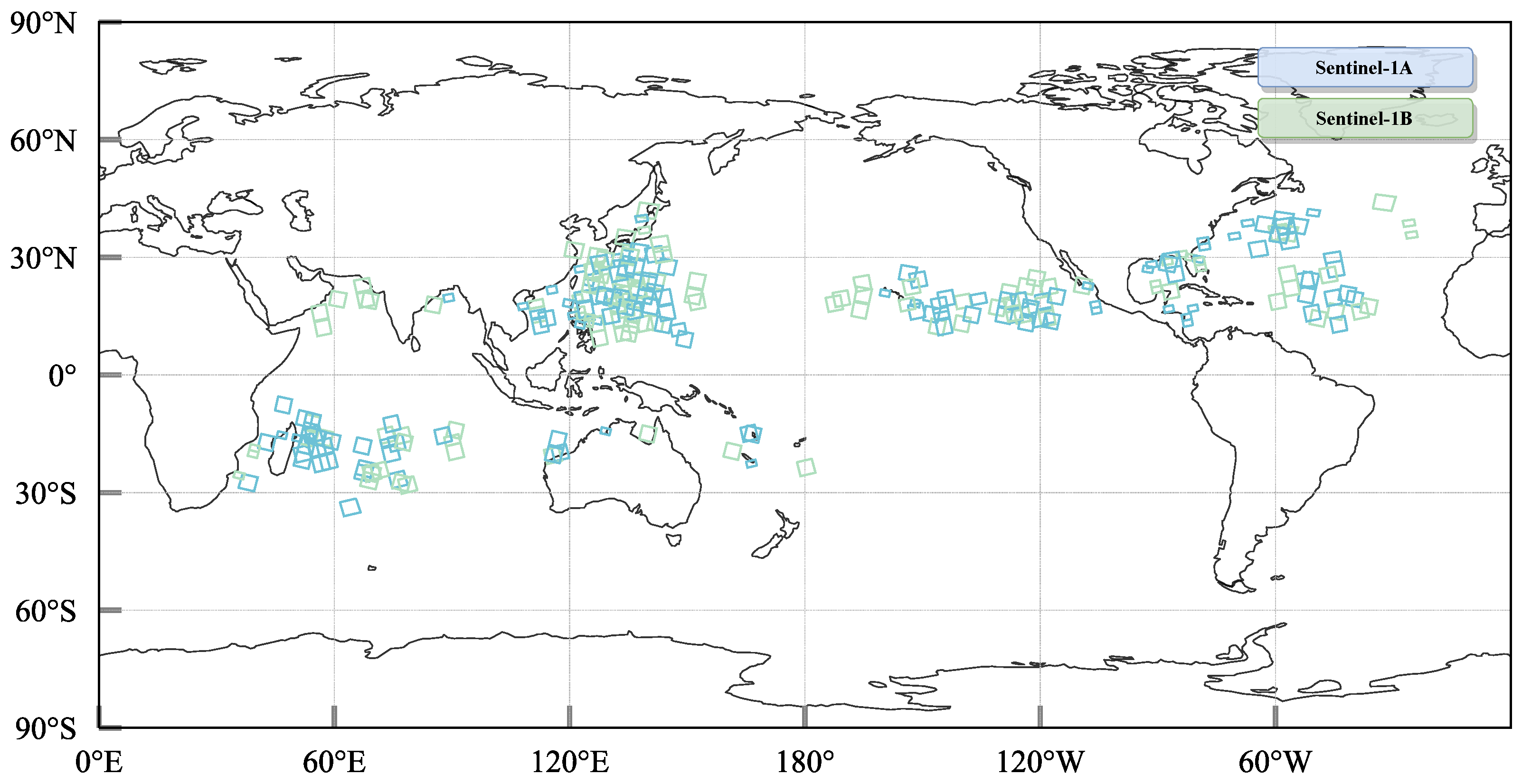
In this study, we collected 270 level-2 ocean (L2 OCN) product SAR wind speeds with a resolution of 1 km as the dataset for SAR wind speed reconstruction. The Sentinel-1 ocean wind field retrieval algorithm is described in [7]. The L2 OCN product also provides an inversion quality flag that classifies the inversion quality of each wind cell in the grid as ‘good’, ‘medium’, ‘low’, or ‘poor’. The geographic locations of the OCN Sentinel-1A/B SAR wind speeds are shown in Figure 7. ECMWF has a resolution of 0.25 degrees (ECMWF provides wind data for a 0.125-degree horizontal grid after the end of 2009) and a time resolution of 3 h. The ECMWF is selected at the closest time to the SAR data acquisition and interpolates to the same resolution as Sentinel-1 [7]. We use ECMWF as labels to train and validate the model and to test Sentinel-1 A/B SAR wind speeds. It is worth noting that during validation and testing, we kept the ‘good’ and ‘medium’ data according to the inversion quality flag and masked the ‘low’ and ‘poor’ data as low-quality data.

3.2. Experiment Configuration and Implementation Details

Our experiments were carried out on a server with an Intel Xeon E5-2680 v4 CPU and two Tesla M60 graphics cards (two cores each), with a total video memory of 32GB. The operating system was Ubuntu 18.04.6, with Python 3.9 and CUDA 11.2.
For the model training, 270 TC images were split into training and validation sets at a ratio of 8:2. We used the Adam optimizer ( β 1 = 0; β 2 = 0.9) and set a batch size of 4 × 10 (multi-GPU training), which is the maximum load of our server. We fed 40 images into the model for each iteration and updated the parameters. We randomly cropped 160 × 160-sized sub-images from ECMWF during training. We also used random smearing to create a mask the same size as the input image and reproduce the problem of SAR low-quality data. The minimum width of the smeared lines is 1 pixel, which helps the model better adapt to the small-sized low-quality parts, and the maximum width is 40 pixels. Moreover, the minimum smearing area is 5%, and the maximum is 75%. This way of creating a mask makes the model generalizable and reduces the possibility of overfitting compared to a fixed mask. In addition, randomly cropped images from each original TC image can also reduce the amount of calculation, which avoids using a too-small batch size on limited computer resources and improves the training speed.
The learning rates for the generator and the discriminator were set to 1 e 4 . After convergence, we reduced the learning rate to 5 e 5 and performed several iterations to achieve better results.

3.3. Evaluation Metric

Considering the difference between RGB data and ours, we carefully chose four evaluation indicators to analyze the reconstruction effect of TCs: the structural similarity index metric (SSIM), the peak signal to noise ratio (PSNR), the root mean square error (RMSE), and the correlation coefficient (R).
Assuming there are images x and y, SSIM can be used to calculate their similarity, whose range is (0–1). The closer the value is to 1, the more similar the images are. SSIM is defined as follows:
S S I M ( x , y ) = ( 2 μ x μ y + C 1 ) ( 2 σ x y + C 2 ) ( μ x 2 + μ y 2 + C 1 ) ( σ x 2 + σ y 2 + C 2 ) .
PSNR is used to evaluate the image quality in units of dB, where larger values indicate less distortion and a better image quality. Letting the original image I and the reconstructed image K have dimensions M × N , PSNR is denoted as:
P S N R = 10 · log 10 ( M A X I 2 1 M N i = 0 m 1 j = 0 n 1 [ I ( i , j ) K ( i , j ) ] 2 ) ,
where M A X I is the maximum value in image I. Before SSIM and PSNR are calculated, the image is first normalized. Both SSIM and PSNR are commonly used evaluation metrics in image inpainting and reconstruction.
Moreover, for TC wind speed data, we use the RMSE, which is an evaluation method that is more common in wind speed inversion tasks:
R M S E = 1 # G G [ I ( i , j ) K ( i , j ) ] 2 ,
where G represents the low-quality regions and # G denotes the number of pixels in this area. In this paper, we only calculate the RMSE for the area that needs to be reconstructed to verify the effect of DeCA-GAN on TC reconstruction.
We also choose R as a key evaluation metric, which is used to measure the degree of linear correlation between variables under study:
R ( X , Y ) = C o v ( X , Y ) V a r [ X ] V a r [ Y ] .

3.4. Experimental Results

In this section, we compare the proposed method with three other state-of-the-art baselines in Section 3.4.1 and directly test our model on Sentinel1-A/B wind speeds in Section 3.4.2. Furthermore, the reconstruction results are further verified with SMAP. To ensure fairness, we use the same hyperparameters for training and validation on ECMWF.
  • PConv [51] proposes to replace vanilla convolution with partial convolution to reduce the color discrepancy in the missing area.
  • GatedConv [50] is a two-stage network: the first stage outputs coarse results and the second stage is for finer ones. This structure can progressively increase the smoothness of the reconstructed image. The work also proposes an SN-PatchGAN for training.
  • AOT-GAN [30] aggregates the feature maps of different receptive fields to improve the reconstruction effect of high-resolution images.

3.4.1. Comparison of DeCA-GAN to Baselines

In this section, we compare the proposed model with three baselines and show the advantages of DeCA-GAN on high wind speeds and large-range low-quality data reconstruction. The quantitative comparison results can be found in Table 1. It shows that our model outperforms the state-of-the-art methods regarding all metrics, especially in the RMSE. Specifically, our model outperforms AOT-GAN [30], the most competitive model.
We conducted two extra quantitative experiments for further verify that the proposed model has better performance on a large range of low-quality data and high wind speed reconstruction. First, we conducted quantitative comparisons under different low-quality data ranges. As shown in Table 2, DeCA-GAN has apparent advantages in reconstructing SAR wind speeds that contain more than 20% low-quality data. Notably, the reconstruction results of the three models (GatedConv, AOT-GAN, and DeCA-GAN) exhibit RMSE values of 1.21 m/s, 1.10 m/s, and 0.95 m/s with under 60–80% of low-quality data, respectively. We find that GatedConv is slightly better than the proposed model regarding PSNR in 0–20% low-quality ranges, but with the increase in low-quality data, the attenuation is more serious. It is worth mentioning that the proposed model outperforms GatedConv in the rest of the metrics. This shows that the proposed model has better stability for reconstructing a large range of low-quality data.
Second, we conducted quantitative comparisons for different wind speed segments, especially for the low and high wind speed parts. As shown in Table 1, the improvements of the proposed model are not very obvious in SSIM and R. This is mainly due to data imbalance in the TC reconstruction task. To explain this, we draw Figure 8 to highlight the advantages of our DeCA-GAN in reconstructing low and high wind speeds. We group the data in the validation set, and each group has a wind speed range of 2 m/s. There are 2,029,266 collocations in low-quality data in our validation set. However, the main structures of a TC (the wind wall and the wind eye, which have wind speeds lower than 2 m/s or greater than 30 m/s) only account for a small part, which makes it difficult for the model to learn the TC structure effectively from the training set. It is not complicated for DL models to reconstruct the wind speed outside the TC that contains a large number of samples, but the TC structure is the primary challenge. This results in the model’s improvement in reconstructing the TC structure being averaged out, and only a slight improvement of DeCA-GAN in SSIM and R. Notably, SSIM evaluates the similarity of the whole image. Non-low-quality data are also involved in the calculation. As shown in Figure 8, we calculated the RMSE under different wind speed segments, showing that the slight improvement in SSIM and R comes from the TC structure. The model has a good reconstruction effect for wind speeds with a large sample size, while for a small sample size, the RMSE is relatively higher. Compared with other models, when the wind speed is lower than 2 m/s or greater than 30 m/s, DeCA-GAN can overcome the data imbalance problem and obtain an improvement of 1.70 m/s in the RMSE at 34–36 m/s wind speeds.

3.4.2. Reconstruction on Sentinel1-A/B

In this section, we directly input Sentinel-1 SAR wind speeds and validated the reconstruction results on ECMWF and SMAP. The results of the proposed method are shown in Figure 9. SAR is affected by rain bands and extreme wind speeds, which generate a large amount of low-quality data and thus make it difficult to observe TCs accurately. We masked ‘low’ and ‘poor’ data as low-quality data based on the quality flags provided in the L2 OCN product. The proposed model is able to enhance the low-quality data of SAR and reconstruct the entire TC structure from the Sentinel-1 SAR wind speeds with results similar to ECMWF. In addition, the proposed model can still predict an accurate structure based on the TC features learned from the training set when the low-quality data region is large, even when the whole TC structure is masked. In particular, low-quality regions including very high wind speeds at the wind wall and low wind speeds in the wind eye can be well reconstructed at the correct locations.
As shown in Table 3, our model can improve the low-quality data in SAR wind speeds and achieve a relative reduction of 50% in the RMSE. Due to the slight time difference between Sentinel-1 SAR image imaging and ECMWF winds, the position and structure of the TC in the image will differ, so the evaluation metric will be reduced accordingly. Specifically, the RMSE is 2.60 m/s, the R is 0.777, the SSIM is 0.907, and the PSNR is 28.02.
To further verify the effectiveness of the proposed model, we also compared the reconstruction results with SMAP data. We searched 25 SMAP datasets to match Sentinel-1 and obtained a total of 5515 matchups. The imaging time difference between these two datasets is within 60 min. The results show that the RMSE of the reconstructed Sentinel-1 image is 3.78 m/s, and the correlation coefficient (R) is 0.79, as shown in Figure 10. These results indicate that the proposed model performs well in reconstructing TCs from SAR wind speeds. However, as shown in the scatter plot in Figure 10, reconstructed high wind speeds (greater than 20 m/s) are significantly underestimated compared to SMAP. We believe this phenomenon is due to the underestimation of strong TC winds in the ECMWF [58,59]. Although the model can reconstruct TC images through learned features, it cannot avoid the limitations of the training set. Thus, the model does not tend to reconstruct extreme winds well, such as those in SMAP data. Additionally, it is worth noting that the RMSE and R values in the comparison are slightly lower than those obtained on the test set, which may be due to imaging time differences in the SMAP data.

3.5. Ablation Studies

We conducted ablation experiments to verify the effectiveness of the three components of DeCA-GAN (i.e., the dual-level encoder, the number of AOT blocks in the neck, and the GAN loss function). To ensure the validity and credibility of the ablation experiments, we use the same training strategy and hyper-parameters as those of the original DeCA-GAN, as well as a fixed random seed.

3.5.1. Dual-Level Encoder

In this paper, we use the CoT self-attention module to build a global branch to enhance the learning ability of the model. As shown in Section 3.6, this global branch mainly learns the structure of the entire TC image. After the global feature map is combined with the local branch, it can help the model achieve great performance in the overall structure and detailed texture. We removed the global branch and used this as the baseline. This baseline uses the same neck and decoder as those of DeCA-GAN, so any improvement can only be due to changes in the encoder. As shown in Table 4, the model using the global branch has better performance, and the RMSE is improved by about 0.16 m/s compared to the baseline.

3.5.2. Number of AOT Blocks

To study the influence of the number of AOT blocks on the model’s learning ability, we changed the neck of the DeCA-GAN model and attempted to stack four, five, six, seven, or eight AOT blocks. Table 5 shows that the number of blocks greatly impacts the performance of the model. Using five AOT blocks in the neck achieves the best results, with an RMSE improvement of about 0.05 m/s compared to the next best design using six blocks.
In addition, in Section 3.6, we visualize the feature map of the network with eight AOT blocks and find that the outputs of the 4th, 5th, and 6th blocks are better, which was also part of our inspiration when designing the DeCA-GAN.

3.5.3. Benefits of Adversarial Loss

Based on a GAN, this paper adopts an adversarial loss to solve the reconstruction blur caused by L1 (or L2) loss and enhance the reconstruction effect. The baseline does not use generator loss or discriminator loss functions. Compared with the proposed DeCA-GAN, the reconstructed results generated by the baseline are significantly worse in all indicators (see Table 6).

3.6. Visualization of DeCA-GAN Internal Feature Maps

In this section, we analyze some intermediate processes of the DeCA-GAN in extracting TC features. The design idea of the encoder is to let the model learn global and local features simultaneously. Through the dual-level fusion and the attention selection of the ECA module, the encoder of the model can learn the key channels and features for reconstructing TCs more comprehensively. For the neck of the DeCA-GAN, AOT blocks can gradually generate a reconstructed sketch and send it to the decoder for up-sampling. We wrote a simple visualization applet to exhibit some feature maps learned by various parts of the model.

3.6.1. Features Learned by the Dual-Level Encoder

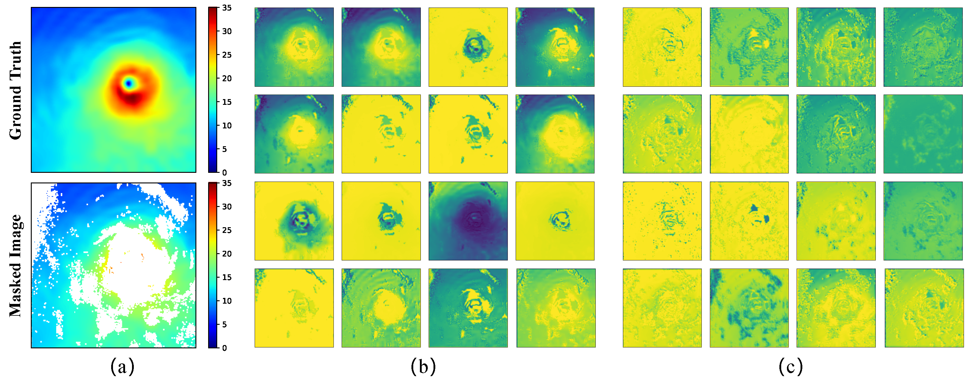
In this part, we show the features extracted by the dual-level encoder and the corresponding masked image in Figure 11a. Figure 11b shows the outputs of the third convolutional layer of the local branch. It can be seen that after three convolutional layers, the network obtains more blurred feature maps. The model pays more attention to extracting local features, especially the distribution of texture features at the edge of the low-quality data, and finds correlation inside and outside the area that needs to be reconstructed. Nevertheless, the feature maps of this branch do not reveal the TC structure. The role of the convolutional layer is to find the relationship between the pixels in the local area, which has a high sensitivity to texture features. However, it is also necessary to learn the overall TC structure from the image for tasks such as TC reconstruction.
As can be seen from the feature maps output by the last CoT block of the global branch in Figure 11c, this branch pays more attention to the content of the entire image than the local branch due to the effect of self-attention module. The pixels that are significant for reconstruction results are given greater weights. Moreover, this branch appears to have learned the ring structure of TCs. These results prove that the global branch can quickly learn the overall TC structure, which could be helpful for the subsequent reconstruction of the neck and up-sampling. Precisely, when the high wind speed parts and the wind eye of the TC are masked, the model must judge the exact wind speed values of the high wind speed area, and the possible position of the wind eye has to be located based on the data that are not masked in the whole image.
With such an encoder design, the two branches of DeCA-GAN can indeed pay attention to global features while preserving local features. This enables the model to perform better on the task of TC reconstruction (see Section 3.5.1).

3.6.2. Feature Integration by AOT Blocks

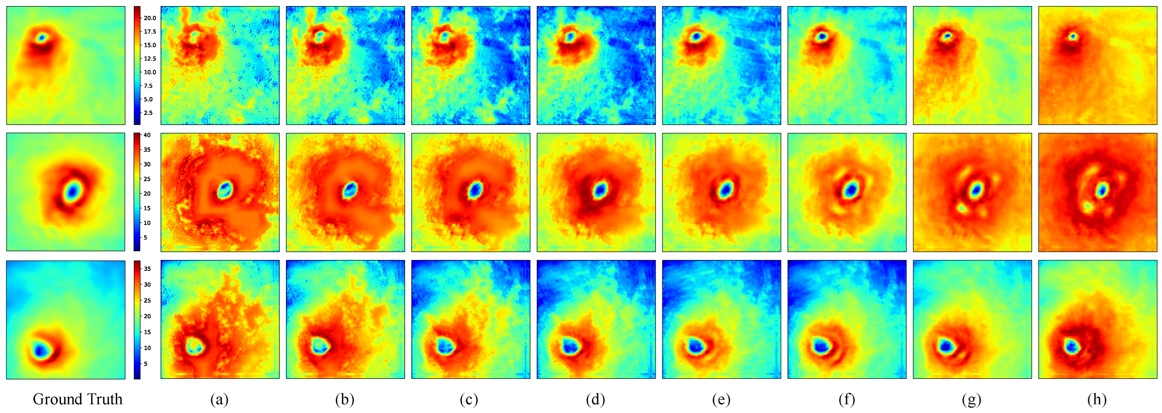
After passing the designed dual-level encoder, the model has learned the local and global features of the image. These learned features are fed into the AOT neck for further processing. The original input size in [30] is 512 × 512 , each AOT block incorporates four receptive fields, and the maximum expansion rate is eight (six is used in this paper), which works well for high-resolution images. However, the image input size of our selection is 160 × 160 , which can contain the entire TC structure; this size is suitable for the dataset studied in this paper and does not require much video memory. In Figure 12, we stack eight AOT blocks in the neck part of the DeCA-GAN to observe the features extracted from each block separately. The colors in Figure 12a–h represent the relative relationships of the different positions extracted by the model. We believe that the number of stacked AOT blocks affects the performance of the network, and we find an interesting phenomenon by visualizing the output of each AOT block.
The features of the first four blocks are relatively elementary, and the structure of TC is distorted and incomplete. The output features of the fifth and sixth AOT blocks are better, and the cyclone center and wind wall are close to the ground truth. From the seventh block, there is a problem with the learned features; the high wind speed area begins to spread, which is inconsistent with the actual situation and the prediction accuracy of the central low-wind area also tends to deteriorate. Therefore, in this paper, the number of AOT blocks is used as a hyper-parameter to conduct ablation experiments, and it is found that the effect is best when using five blocks (see Section 3.5.2).

4. Discussion

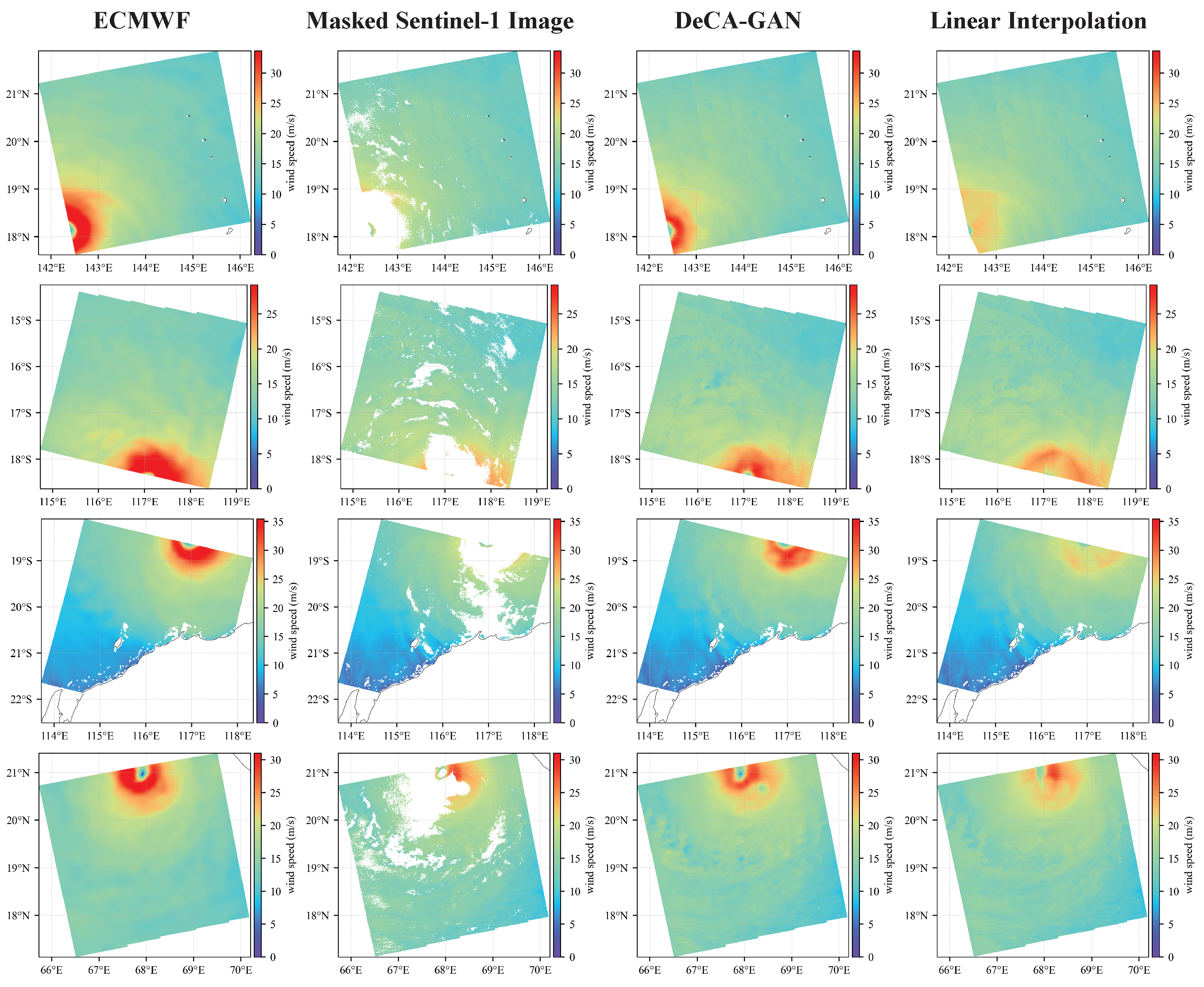
Our designed model can achieve end-to-end SAR wind speed reconstruction in TCs and works well for large low-quality regions and high wind speeds. To further compare the performance of deep learning methods with traditional techniques, we implemented linear and cubic interpolation, obtaining an RMSE of 3.05 m/s and 3.50 m/s, respectively. As shown in Figure 13, when applied to large low-quality regions, linear interpolation tends to be less effective in reconstructing the spatial distribution of tropical cyclones (TCs). This method fails to accurately reconstruct high wind speeds, the wind eye, or the circular structure of TCs, and tends to underestimate wind speeds significantly. In contrast, the deep learning model proposed in this study is able to achieve TC reconstruction, particularly in the case of large low-quality regions of SAR wind speeds. However, there are still some limitations to the performance of this model.
  • We collected 270 ECMWF data and divided them into training and validation sets. However, for DL algorithms, this amount of data is still relatively small. In addition, ECMWF and SAR wind speeds belong to different distributions, resulting in degraded performance when reconstructing SAR observations directly. We will continue to expand the amount of data or introduce some techniques to obtain data closer to the SAR distribution.
  • The DeCA-GAN was trained based on ECMWF wind speed data as labels. ECMWF is a very commonly used dataset in the wind speed retrieval of remote sensing satellites. However, some studies have shown that ECMWF underestimates high wind speeds [58,59], which may lead to some bias in the features learned by the proposed model. This point is also confirmed by the comparison with SMAP, which indicates that our model tends to underestimate wind speeds in high wind speed ranges. The next step is to train the model using the Hurricane Weather Research and Forecasting wind speed.

5. Conclusions

In conclusion, this paper presents a DeCA-GAN model for improving low-quality SAR wind speed data and reconstructing TC structures. The reconstructed results retain the original SAR high-precision wind speed, and only the data in the low-quality region are improved to obtain results that are close to reality. In particular, the model works well for reconstructing high wind speeds and large ranges of low-quality data. The reconstructed results can be used for TC intensity estimation, data assimilation, TC forecast accuracy improvement, TC structure analysis, etc. Furthermore, the DL algorithm is very low-cost and fast.
The proposed method is based on an encoder–neck–decoder architecture, with two parallel branches that combine CNNs and the self-attention mechanism to extract local and global features. The neck part of the model consists of AOT blocks that extract contextual features and send them to the decoder to generate reconstruction results. We also introduce an ECA module to calculate channel attention in the model, which enables cross-channel interactions. In addition, we use a joint loss to improve the model’s performance. Through ablation experiments, we find that the global branch we designed and the selection of the number of AOT modules have positive impacts. We also find that using GAN loss significantly improves the reconstruction ability of the model. When applied to reconstruct SAR wind speeds, the model achieves an RMSE of 2.60 m/s, an R value of 0.777, an SSIM of 0.907, and a PSNR of 28.02, achieving a relative reduction of 50% in the RMSE. Additionally, comparing the reconstructed SAR wind speeds with SMAP data yields an RMSE of 3.78 m/s and an R value of 0.79. Overall, our results suggest that the proposed DeCA-GAN model is a promising approach for reconstructing SAR wind speeds in TCs.

Author Contributions

Conceptualization, X.L. and J.Y.; methodology, X.H., X.L., J.W., and L.R.; software, X.H. and X.L.; validation, X.H., X.L., G.Z., and P.C.; formal analysis, X.L., J.W., and X.H.; investigation, X.L., J.W., and H.F.; writing—original draft preparation, X.H.; writing—review and editing, X.L. and J.Y.; project administration, Q.X. All authors have read and agreed to the published version of the manuscript.

Funding

This work was sponsored by the Oceanic Interdisciplinary Program of Shanghai Jiao Tong University (project number SL2021ZD203), the Scientific Research Fund of the Second Institute of Oceanography, Ministry of Natural Resources of China (grant no. JB2205), the China Postdoctoral Science Foundation (grant no. 2022M723705), preferential support for postdoctoral research projects in Zhejiang Province (grant no. ZJ2022041), the Innovation Group Project of Southern Marine Science and Engineering Guangdong Laboratory (Zhuhai) (no. 311021004), the Zhejiang Provincial Natural Science Foundation of China (grant nos. LGF21D060002, LR21D060002, and LQ21D060001), the Project of State Key Laboratory of Satellite Ocean Environment Dynamics, Second Institute of Oceanography, Ministry of Natural Resources of China (grant no. SOEDZZ2205), the Science and Technology Project of Zhejiang Meteorological Bureau (2021YB07), and the open fund of the State Key Laboratory of Satellite Ocean Environment Dynamics, Second Institute of Oceanography, MNR (no. QNHX2222).

Data Availability Statement

The reconstructed Sentinel-1 A/B wind speeds are available on our Google Drive at: https://drive.google.com/drive/folders/1BVcSoUAj4J4G9qMrjpfQ-9_FwDWRyaGk (accessed on 6 March 2023).

Conflicts of Interest

The authors declare no conflict of interest.

References

  1. Gray, W.M. Tropical Cyclone Genesis. Ph.D. Thesis, Colorado State University, Fort Collins, CO, USA, 1975. [Google Scholar]
  2. Emanuel, K. Tropical cyclones. Annu. Rev. Earth Planet. Sci. 2003, 31, 75–104. [Google Scholar] [CrossRef]
  3. Peduzzi, P.; Chatenoux, B.; Dao, H.; De Bono, A.; Herold, C.; Kossin, J.; Mouton, F.; Nordbeck, O. Global trends in tropical cyclone risk. Nat. Clim. Change 2012, 2, 289–294. [Google Scholar] [CrossRef]
  4. Katsaros, K.B.; Vachon, P.W.; Black, P.G.; Dodge, P.P.; Uhlhorn, E.W. Wind fields from SAR: Could they improve our understanding of storm dynamics? Johns Hopkins APL Tech. Digest 2000, 21, 86–93. [Google Scholar] [CrossRef]
  5. Tiampo, K.F.; Huang, L.; Simmons, C.; Woods, C.; Glasscoe, M.T. Detection of Flood Extent Using Sentinel-1A/B Synthetic Aperture Radar: An Application for Hurricane Harvey, Houston, TX. Remote Sens. 2022, 14, 2261. [Google Scholar] [CrossRef]
  6. Soria-Ruiz, J.; Fernández-Ordoñez, Y.M.; Chapman, B. Radarsat-2 and Sentinel-1 Sar to Detect and Monitoring Flooding Areas in Tabasco, Mexico. In Proceedings of the 2021 IEEE International Geoscience and Remote Sensing Symposium IGARSS, Brussels, Belgium, 11–16 July 2021; pp. 1323–1326. [Google Scholar] [CrossRef]
  7. Sentinel-1 Ocean Wind Fields (OWI) Algorithm Definition. Available online: https://sentinel.esa.int/documents/247904/4766122/DI-MPC-IPF-OWI_2_1_OWIAlgorithmDefinition.pdf/ (accessed on 3 April 2023).
  8. Hwang, P.A.; Zhang, B.; Perrie, W. Depolarized radar return for breaking wave measurement and hurricane wind retrieval. Geophys. Res. Lett. 2010, 37. [Google Scholar] [CrossRef]
  9. Vachon, P.W.; Wolfe, J. C-band cross-polarization wind speed retrieval. IEEE Geosci. Remote Sens. Lett. 2010, 8, 456–459. [Google Scholar] [CrossRef]
  10. de Kloe, J.; Stoffelen, A.; Verhoef, A. Improved use of scatterometer measurements by using stress-equivalent reference winds. IEEE J. Sel. Top. Appl. Earth Obs. Remote Sens. 2017, 10, 2340–2347. [Google Scholar] [CrossRef]
  11. Shen, H.; Perrie, W.; He, Y.; Liu, G. Wind speed retrieval from VH dual-polarization RADARSAT-2 SAR images. IEEE Trans. Geosci. Remote Sens. 2013, 52, 5820–5826. [Google Scholar] [CrossRef]
  12. Zhang, B.; Perrie, W. Cross-polarized synthetic aperture radar: A new potential measurement technique for hurricanes. Bull. Am. Meteorol. Soc. 2012, 93, 531–541. [Google Scholar] [CrossRef]
  13. Zhang, G.; Li, X.; Perrie, W.; Hwang, P.A.; Zhang, B.; Yang, X. A hurricane wind speed retrieval model for C-band RADARSAT-2 cross-polarization ScanSAR images. IEEE Trans. Geosci. Remote Sens. 2017, 55, 4766–4774. [Google Scholar] [CrossRef]
  14. Zhang, G.; Perrie, W. Symmetric double-eye structure in hurricane bertha (2008) imaged by SAR. Remote Sens. 2018, 10, 1292. [Google Scholar] [CrossRef]
  15. Zhang, G.; Perrie, W.; Zhang, B.; Yang, J.; He, Y. Monitoring of tropical cyclone structures in ten years of RADARSAT-2 SAR images. Remote Sens. Environ. 2020, 236, 111449. [Google Scholar] [CrossRef]
  16. Zhang, B.; Zhu, Z.; Perrie, W.; Tang, J.; Zhang, J.A. Estimating tropical cyclone wind structure and intensity from spaceborne radiometer and synthetic aperture radar. IEEE J. Sel. Top. Appl. Earth Obs. Remote Sens. 2021, 14, 4043–4050. [Google Scholar] [CrossRef]
  17. Portabella, M.; Stoffelen, A.; Johannessen, J.A. Toward an optimal inversion method for synthetic aperture radar wind retrieval. J. Geophys. Res. Oceans 2002, 107, 1-1-1-13. [Google Scholar] [CrossRef]
  18. Ye, X.; Lin, M.; Zheng, Q.; Yuan, X.; Liang, C.; Zhang, B.; Zhang, J. A typhoon wind-field retrieval method for the dual-polarization SAR imagery. IEEE Geosci. Remote Sens. Lett. 2019, 16, 1511–1515. [Google Scholar] [CrossRef]
  19. Boussioux, L.; Zeng, C.; Guénais, T.; Bertsimas, D. Hurricane forecasting: A novel multimodal machine learning framework. Weather Forecast. 2022, 37, 817–831. [Google Scholar] [CrossRef]
  20. Carmo, A.R.; Longépé, N.; Mouche, A.; Amorosi, D.; Cremer, N. Deep Learning Approach for Tropical Cyclones Classification Based on C-Band Sentinel-1 SAR Images. In Proceedings of the 2021 IEEE International Geoscience and Remote Sensing Symposium IGARSS, Brussels, Belgium, 11–16 July 2021; pp. 3010–3013. [Google Scholar] [CrossRef]
  21. Li, X.M.; Qin, T.; Wu, K. Retrieval of sea surface wind speed from spaceborne SAR over the Arctic marginal ice zone with a neural network. Remote Sens. 2020, 12, 3291. [Google Scholar] [CrossRef]
  22. Funde, K.; Joshi, J.; Damani, J.; Jyothula, V.R.; Pawar, R. Tropical Cyclone Intensity Classification Using Convolutional Neural Networks On Satellite Imagery. In Proceedings of the 2022 International Conference on Industry 4.0 Technology (I4Tech), Pune, India, 23–24 September 2022; pp. 1–5. [Google Scholar] [CrossRef]
  23. Yu, P.; Xu, W.; Zhong, X.; Johannessen, J.A.; Yan, X.H.; Geng, X.; He, Y.; Lu, W. A Neural Network Method for Retrieving Sea Surface Wind Speed for C-Band SAR. Remote Sens. 2022, 14, 2269. [Google Scholar] [CrossRef]
  24. Mu, S.; Li, X.; Wang, H. The Fusion of Physical, Textural and Morphological Information in SAR Imagery for Hurricane Wind Speed Retrieval Based on Deep Learning. IEEE Trans. Geosci. Remote Sens. 2022, 60, 1–13. [Google Scholar] [CrossRef]
  25. Nezhad, M.M.; Heydari, A.; Pirshayan, E.; Groppi, D.; Garcia, D.A. A novel forecasting model for wind speed assessment using sentinel family satellites images and machine learning method. Renew. Energy 2021, 179, 2198–2211. [Google Scholar] [CrossRef]
  26. Goodfellow, I.J.; Pouget-Abadie, J.; Mirza, M.; Xu, B.; Warde-Farley, D.; Ozair, S.; Courville, A.C.; Bengio, Y. Generative Adversarial Nets. In Proceedings of the Advances in Neural Information Processing Systems 27: Annual Conference on Neural Information Processing Systems 2014, Montreal, QC, Canada, 8–13 December 2014; pp. 2672–2680. [Google Scholar]
  27. Yu, F.; Koltun, V. Multi-Scale Context Aggregation by Dilated Convolutions. In Proceedings of the 4th International Conference on Learning Representations, San Juan, Puerto Rico, 2–4 May 2016. [Google Scholar]
  28. Vaswani, A.; Shazeer, N.; Parmar, N.; Uszkoreit, J.; Jones, L.; Gomez, A.N.; Kaiser, L.; Polosukhin, I. Attention is All you Need. In Proceedings of the Advances in Neural Information Processing Systems 30: Annual Conference on Neural Information Processing Systems 2017, Long Beach, CA, USA, 4–9 December 2017; pp. 5998–6008. [Google Scholar]
  29. Li, Y.; Yao, T.; Pan, Y.; Mei, T. Contextual transformer networks for visual recognition. IEEE Trans. Pattern Anal. Mach. Intell. 2022, 45, 1489–1500. [Google Scholar] [CrossRef]
  30. Zeng, Y.; Fu, J.; Chao, H.; Guo, B. Aggregated contextual transformations for high-resolution image inpainting. IEEE Trans. Visual Comput. Graphics 2022. [Google Scholar] [CrossRef]
  31. Wang, Q.; Wu, B.; Zhu, P.; Li, P.; Zuo, W.; Hu, Q. ECA-Net: Efficient Channel Attention for Deep Convolutional Neural Networks. In Proceedings of the 2020 IEEE/CVF Conference on Computer Vision and Pattern Recognition, CVPR 2020, Seattle, WA, USA, 13–19 June 2020; pp. 11531–11539. [Google Scholar] [CrossRef]
  32. Wang, P.; Chen, P.; Yuan, Y.; Liu, D.; Huang, Z.; Hou, X.; Cottrell, G. Understanding convolution for semantic segmentation. In Proceedings of the 2018 IEEE Winter Conference on Applications of Computer Vision (WACV), Lake Tahoe, NV, USA, 12–15 March 2018; pp. 1451–1460. [Google Scholar] [CrossRef]
  33. Mottaghi, R.; Chen, X.; Liu, X.; Cho, N.; Lee, S.; Fidler, S.; Urtasun, R.; Yuille, A.L. The Role of Context for Object Detection and Semantic Segmentation in the Wild. In Proceedings of the 2014 IEEE Conference on Computer Vision and Pattern Recognition, CVPR 2014, Columbus, OH, USA, 23–28 June 2014; pp. 891–898. [Google Scholar] [CrossRef]
  34. Rabinovich, A.; Vedaldi, A.; Galleguillos, C.; Wiewiora, E.; Belongie, S.J. Objects in Context. In Proceedings of the IEEE 11th International Conference on Computer Vision, ICCV 2007, Rio de Janeiro, Brazil, 14–20 October 2007; pp. 1–8. [Google Scholar] [CrossRef]
  35. Zeng, X.; Ouyang, W.; Wang, X. Multi-stage Contextual Deep Learning for Pedestrian Detection. In Proceedings of the IEEE International Conference on Computer Vision, ICCV 2013, Sydney, Australia, 1–8 December 2013; pp. 121–128. [Google Scholar] [CrossRef]
  36. Tan, Z.; Wang, M.; Xie, J.; Chen, Y.; Shi, X. Deep Semantic Role Labeling With Self-Attention. In Proceedings of the AAAI (Thirty-Second AAAI Conference on Artificial Intelligence), New Orleans, LA, USA, 2–7 February 2018; pp. 4929–4936. [Google Scholar]
  37. Verga, P.; Strubell, E.; McCallum, A. Simultaneously Self-Attending to All Mentions for Full-Abstract Biological Relation Extraction. In Proceedings of the NAACL-HLT (North American Chapter of the Association for Computational Linguistics: Human Language Technologies), New Orleans, LA, USA, 1–6 June 2018; pp. 872–884. [Google Scholar] [CrossRef]
  38. Devlin, J.; Chang, M.W.; Lee, K.; Toutanova, K. BERT: Pre-training of Deep Bidirectional Transformers for Language Understanding. In Proceedings of the NAACL-HLT 2019, Minneapolis, MN, USA, 2–7 June 2019; pp. 4171–4186. [Google Scholar] [CrossRef]
  39. Dosovitskiy, A.; Beyer, L.; Kolesnikov, A.; Weissenborn, D.; Zhai, X.; Unterthiner, T.; Dehghani, M.; Minderer, M.; Heigold, G.; Gelly, S.; et al. An image is worth 16x16 words: Transformers for image recognition at scale. arXiv 2020, arXiv:2010.11929. [Google Scholar]
  40. Carion, N.; Massa, F.; Synnaeve, G.; Usunier, N.; Kirillov, A.; Zagoruyko, S. End-to-end object detection with transformers. In Computer Vision–ECCV 2020: Proceedings of the 16th European Conference, Glasgow, UK, 23–28 August 2020; Springer: Berlin/Heidelberg, Germany, 2020; pp. 213–229. [Google Scholar]
  41. Liu, Z.; Lin, Y.; Cao, Y.; Hu, H.; Wei, Y.; Zhang, Z.; Lin, S.; Guo, B. Swin transformer: Hierarchical vision transformer using shifted windows. In Proceedings of the IEEE/CVF International Conference on Computer Vision, Montreal, BC, Canada, 11–17 October 2021; pp. 10012–10022. [Google Scholar] [CrossRef]
  42. Ramachandran, P.; Parmar, N.; Vaswani, A.; Bello, I.; Levskaya, A.; Shlens, J. Stand-alone self-attention in vision models. Adv. Neural Inf. Process. Syst. 2019, 32. [Google Scholar]
  43. Zhao, H.; Jia, J.; Koltun, V. Exploring Self-Attention for Image Recognition. In Proceedings of the 2020 IEEE/CVF Conference on Computer Vision and Pattern Recognition, CVPR 2020, Seattle, WA, USA, 13–19 June 2020; pp. 10073–10082. [Google Scholar] [CrossRef]
  44. He, K.; Zhang, X.; Ren, S.; Sun, J. Deep Residual Learning for Image Recognition. In Proceedings of the 2016 IEEE Conference on Computer Vision and Pattern Recognition, CVPR 2016, Las Vegas, NV, USA, 27–30 June 2016; pp. 770–778. [Google Scholar] [CrossRef]
  45. Xie, S.; Girshick, R.B.; Dollár, P.; Tu, Z.; He, K. Aggregated Residual Transformations for Deep Neural Networks. In Proceedings of the 2017 IEEE Conference on Computer Vision and Pattern Recognition, CVPR 2017, Honolulu, HI, USA, 21–26 July 2017; pp. 5987–5995. [Google Scholar] [CrossRef]
  46. Zhang, H.; Wu, C.; Zhang, Z.; Zhu, Y.; Lin, H.; Zhang, Z.; Sun, Y.; He, T.; Mueller, J.; Manmatha, R.; et al. Resnest: Split-attention networks. In Proceedings of the IEEE/CVF Conference on Computer Vision and Pattern Recognition, New Orleans, LA, USA, 18–24 June 2022; pp. 2736–2746. [Google Scholar]
  47. Hu, J.; Shen, L.; Sun, G. Squeeze-and-Excitation Networks. In Proceedings of the 2018 IEEE Conference on Computer Vision and Pattern Recognition, CVPR 2018, Salt Lake City, UT, USA, 18–22 June 2018; pp. 7132–7141. [Google Scholar] [CrossRef]
  48. Tan, M.; Le, Q.V. EfficientNet: Rethinking Model Scaling for Convolutional Neural Networks. In Proceedings of the International Conference on Machine Learning 2019, Long Beach, CA, USA, 9–15 June 2019; Volume 97, pp. 6105–6114. [Google Scholar]
  49. Woo, S.; Park, J.; Lee, J.Y.; Kweon, I.S. Cbam: Convolutional block attention module. In Proceedings of the European conference on computer vision (ECCV), Munich, Germany, 8–14 September 2018; pp. 3–19. [Google Scholar]
  50. Yu, J.; Lin, Z.; Yang, J.; Shen, X.; Lu, X.; Huang, T.S. Free-Form Image Inpainting With Gated Convolution. In Proceedings of the 2019 IEEE/CVF International Conference on Computer Vision, ICCV 2019, Seoul, Republic of Korea, 27 October–2 November 2019; pp. 4470–4479. [Google Scholar] [CrossRef]
  51. Liu, G.; Reda, F.A.; Shih, K.J.; Wang, T.C.; Tao, A.; Catanzaro, B. Image inpainting for irregular holes using partial convolutions. In Proceedings of the European conference on computer vision (ECCV), Munich, Germany, 8–14 September 2018; pp. 85–100. [Google Scholar] [CrossRef]
  52. Yu, J.; Lin, Z.; Yang, J.; Shen, X.; Lu, X.; Huang, T.S. Generative Image Inpainting With Contextual Attention. In Proceedings of the 2018 IEEE Conference on Computer Vision and Pattern Recognition, CVPR 2018, Salt Lake City, UT, USA, 18–22 June 2018; pp. 5505–5514. [Google Scholar] [CrossRef]
  53. Isola, P.; Zhu, J.; Zhou, T.; Efros, A.A. Image-to-Image Translation with Conditional Adversarial Networks. In Proceedings of the 2017 IEEE Conference on Computer Vision and Pattern Recognition, CVPR 2017, Honolulu, HI, USA, 21–26 July 2017; pp. 5967–5976. [Google Scholar] [CrossRef]
  54. Gatys, L.A.; Ecker, A.S.; Bethge, M. Image Style Transfer Using Convolutional Neural Networks. In Proceedings of the 2016 IEEE Conference on Computer Vision and Pattern Recognition, CVPR 2016, Las Vegas, NV, USA, 27–30 June 2016; pp. 2414–2423. [Google Scholar] [CrossRef]
  55. Johnson, J.; Alahi, A.; Fei-Fei, L. Perceptual losses for real-time style transfer and super-resolution. In Computer Vision–ECCV 2016: Proceedings of the 14th European Conference, Amsterdam, The Netherlands, 11–14 October 2016; Springer: Berlin/Heidelberg, Germany, 2016; pp. 694–711. [Google Scholar] [CrossRef]
  56. Simonyan, K.; Zisserman, A. Very Deep Convolutional Networks for Large-Scale Image Recognition. In Proceedings of the 3rd International Conference on Learning Representations (ICLR 2015), San Diego, CA, USA, 7–9 May 2015. [Google Scholar]
  57. Njoku, E.; Entekhabi, D.; Kellogg, K.; O’Neill, P. The Soil Moisture Active and Passive (SMAP) Mission. Earth Obs. Water Cycle Sci. 2009, 674, 2. [Google Scholar]
  58. Li, X.; Yang, J.; Wang, J.; Han, G. Evaluation and Calibration of Remotely Sensed High Winds from the HY-2B/C/D Scatterometer in Tropical Cyclones. Remote Sens. 2022, 14, 4654. [Google Scholar] [CrossRef]
  59. Li, X.; Yang, J.; Han, G.; Ren, L.; Zheng, G.; Chen, P.; Zhang, H. Tropical Cyclone Wind Field Reconstruction and Validation Using Measurements from SFMR and SMAP Radiometer. Remote Sens. 2022, 14, 3929. [Google Scholar] [CrossRef]
Figure 1. An overview of the Dual-Level Contextual Attention Network (DeCA-GAN) architecture. The DeCA-GAN is built with a generator and a discriminator. The encoder of the generator is a two-branch network for extracting features at the local and global levels, respectively, and the neck consists of five feature extractors for progressively generating contours of the TC structure. The discriminator uses the original mask as a label for the task of predicting patch-level pixels.
Remotesensing 15 02454 g001
Figure 2. Structure of the (a) CoT Block and (b) CoT in the DeCA-GAN.
Remotesensing 15 02454 g002
Figure 3. Illustration of the self-attention mechanism in the DeCA-GAN.
Remotesensing 15 02454 g003
Figure 4. The structure of the ECA module.
Remotesensing 15 02454 g004
Figure 5. The structure of the AOT block. The four terms inside the green and gray rectangles represent the number of input channels, the size of the convolutional kernel, the dilation rate, and the number of output channels, respectively.
Remotesensing 15 02454 g005
Figure 6. Diagram of the SM-PatchGAN architecture for SAR wind speed reconstruction.
Remotesensing 15 02454 g006
Figure 7. Geographical location of 270 Sentinel-1A/B images including TC structure. The blue and green rectangles denote images from Sentinel-1A (147 images) and Sentinel-1B (123 images), respectively.
Remotesensing 15 02454 g007
Figure 8. Quantitative comparisons of the RMSE (curve) and number of collocations (histogram) for different wind speed ranges.
Remotesensing 15 02454 g008
Figure 9. Comparisons of DeCA-GAN-reconstructed Sentinel-1-A/B SAR wind speeds with ECMWF and original SAR wind speeds. (a) ECMWF; (b) original SAR wind speeds; (c) masked SAR wind speeds; (d) reconstructed SAR wind speeds.
Remotesensing 15 02454 g009
Figure 10. Comparisons of the Sentinel-1-A/B SAR wind speeds reconstructed by the DeCA-GAN with the SMAP radiometer winds.
Remotesensing 15 02454 g010
Figure 11. Feature maps learned by the dual-level encoder. (a) The input masked image and the corresponding ground truth. (b) Local branch. (c) Global branch.
Remotesensing 15 02454 g011
Figure 12. Visualization of the neck of the DeCA-GAN. The image features extracted by each AOT block from ground truth are visualized in (ah). The color range of each feature map is kept consistent and is set according to the maximum and minimum values of all feature maps.
Remotesensing 15 02454 g012
Figure 13. Comparison of the DeCA-GAN and the linear interpolation method.
Remotesensing 15 02454 g013
Table 1. Quantitative comparisons of proposed DeCA-GAN and other state-of-the-art models on the validation set. ↑ Higher is better. ↓ Lower is better.
MethodsSSIM ↑PSNR ↑RMSE ↓R↑
PConv0.99041.051.180.947
GatedConv0.99142.870.960.970
AOT-GAN0.99141.490.950.970
DeCA-GAN (ours)0.99443.810.740.983
Table 2. Quantitative comparisons of the proposed DeCA-GAN and other state-of-the-art models under different low-quality data ranges. ↑ Higher is better. ↓ Lower is better.
MethodsLow-Quality DataSSIM ↑PSNR ↑RMSE ↓R ↑
GatedConv0–20%0.99646.740.740.982
20–40%0.99642.200.770.982
40–60%0.98836.661.110.962
60–80%0.98333.661.210.945
AOT-GAN0–20%0.99543.340.590.988
20–40%0.99443.070.900.973
40–60%0.99036.621.000.967
60–80%0.98334.361.100.953
DeCA-GAN (ours)0–20%0.99746.430.530.991
20–40%0.99744.310.620.988
40–60%0.99439.070.800.983
60–80%0.98735.780.950.968
Table 3. Performance comparisons of reconstructed and original Sentinel-1 SAR wind speeds. ↑ Higher is better. ↓ Lower is better.
SAR Wind SpeedsSSIM ↑PSNR ↑RMSE ↓R ↑
Original0.80723.255.160.547
Reconstructed0.90728.022.600.777
Table 4. Comparing network performance using a dual-level branch and only a local branch. ↑ Higher is better. ↓ Lower is better.
BranchSSIM ↑PSNR ↑RMSE ↓R ↑
Only Local0.99242.120.900.974
Local and Global0.99443.810.740.983
Table 5. Comparison of results using different AOT block numbers in the DeCA-GAN neck. ↑ Higher is better. ↓ Lower is better.
# BlocksSSIM ↑PSNR ↑RMSE ↓R ↑
40.99140.571.020.971
50.99443.810.740.983
60.99343.410.790.981
70.99343.360.820.977
80.99141.490.940.967
Table 6. Comparison of the results before and after using the GAN loss. ↑ Higher is better. ↓ Lower is better.
LossSSIM ↑PSNR ↑RMSE ↓R ↑
Without GAN0.95535.091.600.909
Ours0.99443.810.740.983
Disclaimer/Publisher’s Note: The statements, opinions and data contained in all publications are solely those of the individual author(s) and contributor(s) and not of MDPI and/or the editor(s). MDPI and/or the editor(s) disclaim responsibility for any injury to people or property resulting from any ideas, methods, instructions or products referred to in the content.