Article

QMRNet: Quality Metric Regression for EO Image Quality Assessment and Super-Resolution

1
Eurecat, Centre Tecnològic de Catalunya, Tecnologies Multimèdia, 08005 Barcelona, Spain
2
Satellogic Inc., Davidson, NC 28036, USA
*
Author to whom correspondence should be addressed.
These authors contributed equally to this work.
Remote Sens. 2023, 15(9), 2451; https://doi.org/10.3390/rs15092451
Submission received: 3 April 2023 / Revised: 27 April 2023 / Accepted: 29 April 2023 / Published: 6 May 2023
(This article belongs to the Special Issue Artificial Intelligence in Computational Remote Sensing)

Abstract

:
The latest advances in super-resolution have been tested with general-purpose images such as faces, landscapes and objects, but mainly unused for the task of super-resolving earth observation images. In this research paper, we benchmark state-of-the-art SR algorithms for distinct EO datasets using both full-reference and no-reference image quality assessment metrics. We also propose a novel Quality Metric Regression Network (QMRNet) that is able to predict the quality (as a no-reference metric) by training on any property of the image (e.g., its resolution, its distortions, etc.) and also able to optimize SR algorithms for a specific metric objective. This work is part of the implementation of the framework IQUAFLOW, which has been developed for the evaluation of image quality and the detection and classification of objects as well as image compression in EO use cases. We integrated our experimentation and tested our QMRNet algorithm on predicting features such as blur, sharpness, snr, rer and ground sampling distance and obtained validation medRs below 1.0 (out of N = 50) and recall rates above 95%. The overall benchmark shows promising results for LIIF, CAR and MSRN and also the potential use of QMRNet as a loss for optimizing SR predictions. Due to its simplicity, QMRNet could also be used for other use cases and image domains, as its architecture and data processing is fully scalable.

1. Introduction

One of the main issues in observing and analyzing earth observation (EO) images is to estimate its quality. However, this main issue is twofold. First, images are captured with distinct image modifications and distortions, such as optical diffractions and aberrations, detector spacing and footprints, atmospheric turbulence, platform vibration, blurring, target motion, and postprocessing. Second, EO image resolution is very limited due to the sensor’s optical resolution, the satellite’s and connection’s capacity to send high-quality images to the ground as well as the captured ground sampling distance (GSD) [1]. These limitations make the image quality assessment (IQA) hard to evaluate for EO particularly, as there are no comparable fine-grained baselines in broad EO domains.
We will tackle these problems by defining a network that acts as a no-reference (blind) metric, assessing the quality and optimizing the super-resolution of EO images at any scale and modification.
Below are summarized our main contributions:
  • We train and validate a novel network (QMRNet) for EO imagery that is able to predict any type of image based on its quality and distortion
  • (Case 1) We benchmark distinct super-resolution models with QMRNet and compare the results with full-reference, no-reference and feature-based metrics
  • (Case 2) We benchmark distinct EO datasets with QMRNet scores
  • (Case 3) We propose to use QMRNet as a loss for optimizing the quality of super-resolution models
Super-resolution (SR) consists of estimating a high-resolution image ( I H R ) given a low-resolution one ( I L R ). In the deep learning era, deep networks have been used to classify images, obtaining a high precision in their predictions. For the specific SR task, one can design a network (autoencoder) whose convolutional layers (feature extractor) encode the patches of the image in order to build a feature vector (encoder) from the image, then add deconvolutional layers to reconstruct the original image (decoder). The instances of the predicted images are compared with the original ones in order to re-train the autoencoder network until they converge to an HR objective. The SRCNN and FSRCNN models [2,3] are based on a network of three blocks (patch extraction and representation, nonlinear mapping and reconstruction). The authors also mention the use of rotation, scaling and noise transformations as data augmentation prior to training the network. The authors use downscaling with a low-pass filter to obtain the I L R images and use a bicubic interpolation for the upscaling during reconstruction to obtain the I S R (the model’s prediction of I H R ). SRCNN has been used by MC-SRCNN [4] to super-resolve multi-spectral images by changing the architecture’s input channels and adding pan-sharpening filters (modulating the smoothing/sharpening intensity). These design principles used in autoencoders, however, have a drawback in that they work differently over feature-size frequencies and features at distinct resolutions. For that, multi-scale architectures are proposed. The Multi-Scale Residual Network (MSRN) [5] uses residual connections in multiple residual blocks at different scale bands, non-exclusive to ResNets. It ables the equalization of the information bottleneck in deeper layers (high-level features) where the spatial information in some cases tends to diminish or either vanish. Traditional convolutional filters in primary layers have a fixed and narrow field of view, which creates dependencies to the learning of spatial long-range connections and deeper layers. However, multi-scale blocks cope with this drawback by analyzing the image domain at different resolution scales to be later merged in a high-dimensional multiband latent space. This allows a better abstraction at deeper layers and, therefore, the reconstruction of spatial information. This is a remarkable advantage when using EO images, which come with distinct resolutions and GSD.
Novel state-of-the-art SR models are based on generative adversarial networks (GANs). These networks are composed of two networks, a generator that generates an image estimate (SR) and a discriminator that decides whether the generated image is real or fake under certain categorical or metric objectives with respect to the classification of a set of images “I”. Usually, the generator is a deconvolutional network that is fed with a latent vector that represents the distribution for each image. In the SR problem, the LR ( I L R ) is considered as the input latent space while the HR image is considered as the real image I H R to obtain the adversarial loss. For the case of the popular SRGAN [6], it has been designed with adversarial loss through VGG and ResNet (SRResnet) with residual connections and perceptual loss. The ESRGAN [7] is an improved version of the SRGAN, although it uses adversarial loss relaxation, adds training upon perceptual loss and has some some residual connections in its architecture. The main intrinsic difference between GANs and other architectures is that the image probability distribution is intrinsically learned. This makes these architectures suffer from unknown artifacts and hallucinations; however, their SR estimates are usually sharper than autoencoder-type architectures. Some mentioned generative techniques for SR, such as SRGAN/SRResnet, ESRGAN and Enlighten-GAN [8], and convolutional SR autoencoders, such as VDSR [9], SRCNN/FRSCNN and MSRN, do not adapt their feature generation to optimize a loss based on a specific quality standard that considers all quality properties of the image (both structural and pixel-to-pixel). However, the predictions show typical distortions such as blurring (from downscaling the input) or GAN artifacts from the training domain objective. Most of these GAN-based models build the I L R inputs of the network from downsampled data from the original I H R . This I L R generation from downsampling I H R limits the training of these models to perform the reverse transformation of the modification; however, the type of distortions and variations from any test image are a combination of much more diverse modifications. The only way to mitigate this limitation, but only partially due to overfitting, is to augment the I L R samples to distinct transformations simultaneously.
Some self-supervised techniques can learn to solve the ill-posed inverse problem from the observed measurements, without any knowledge of the underlying distribution assuming its invariance to the transformations. The Content Adaptive Resampler (CAR) [10] was proposed, in which a join-learnable downscaling pre-step block together with an upscaling block (SRNet) is trained separately. It is able to learn the downscaling step (through a ResamplerNet) by learning the statistics of kernels from the I H R , then it learns the upscaling blocks with another net (SRNet/EDSR) to obtain the SR images. CAR has been able to improve the experimental results of SR by considering the intrinsic divergences between I L R and I H R . The Local Implicit Image Function (LIIF) [11] is able to generate super-resolved pixels considering 2D deep features around these coordinates as inputs. In LIIF, an encoder is jointly trained in a self-supervised super-resolution task maintaining high fidelity at higher resolutions. Since the coordinates are continuous, LIIF can be presented in any arbitrary resolution. Here, the main advantage is that the SR is represented in a resolution without resizing I H R , making it invariant to the transformations performed to the I L R . This enables LIIF to extrapolate SR upon factors up to x30.
In order to assess the quality of an image, there are distinct strategies. Full-reference metrics consider the difference between an estimated or modified image ( I S R ) and the reference image ( I H R ). In contrast, no-reference metrics assess the specific statistical properties of the estimated image without any reference image. Other more novel metrics calculate the high-level characteristics of the estimated I S R by comparing its distribution distance with respect to either a preprocessed dataset or the reference I H R in a feature-based space.
The similarity between the predicted images I S R and the reference high-resolution images I H R is estimated by looking at the pixel-wise differences responsive to reflectance, sharpness, structure, noise, etc. Very well-known examples of pixel-level (or full-reference) metrics are the root-mean-square error (RMSE) [12], Spearman’s rank order correlation coefficient (SRCC or SROCC), Pearson’s linear correlation coefficient (PLCC), Kendall’s rank order correlation coefficient (KROCC), the peak signal-to-noise ratio (PSNR) [13], the structural similarity metric (SSIM/MSSIM) [14], the Haar perceptual similarity index (HAARPSI) [15], the gradient magnitude similarity deviation (GMSD) [16] and the mean deviation similarity index (MDSI) [17]. PSNR calculates the power of the signal-to-noise ratio considering the noise error with respect to the I H R . Some metrics such as the SSIM specifically measure the means and covariances locally for each region at a specific size (e.g., 8 × 8 patches; multi-scale patches for MSSIM) affecting the overall metric score. The GMSD calculates the global variation similarity of the gradient based on a local quality map combined with a pooling strategy. Most comparative studies use these metrics to measure the actual I S R quality, mostly relying on PSNR, although there is no evidence that these measurements are the best for EO cases, as some of these are not sensitive to local perturbations (i.e., blurring, over-sharpening) and local changes (i.e., artifacts, hallucinations) to the image. The HAARPSI calculates an index based on the difference (absolute or in mutual information) using the sum of a set of wavelet coefficients processed over the I S R - I H R images. Other cases of metrics combine some of the pinpointed parameters simultaneously. For instance, the MDSI compares jointly the gradient similarity, chromaticity similarity and deviation pooling. The latest metric design, LCSA [18], uses linear combinations of full-reference metrics, i.e., VSI, FSIM, IFC, MAD, MSSSIM, NQM, PSNR, SSIM and VIF.
Pixel-reference metrics have a main requirement, which is that the ground-truth HR images are needed to assess a specific quality standard. For the case of no-reference (or blind) metrics, no explicit reference is needed. These rely on a parametric characterization of the enhanced signal based on statistic descriptors, usually linked to the noise or sharpness, embedded in high-frequency bands. Some examples are the variance, entropy (He), or high-end spectrum (FFT). The main popular metric in EO is the modulation transfer function (MTF), which measures impulse responses in the spatial domain and transfer functions in the frequency domain. This varies upon overall local pixel characteristics mostly present on contours, corners and sharp features in general [19]. Here, the MTF is very sensitive to local changes such as those aforementioned (e.g., optical diffractions and aberrations, blurring, motion, etc). Other metrics would use statistics from image patches in combination with multivariate filtering methods to propose score indexes for a given predefined image given its geo-referenced parameter standards. Such methods include NIQE [20], PIQE [21] and GIQE [22]. The latter is considered for official evaluation of NIIRS ratings (https://irp.fas.org/imint/niirs.htm, accessed on 10 October 2022) considering the ground sampling distance (GSD), the signal-to-noise ratio (SNR) and the relative edge response (RER) in distinct effective focal lengths of EO images [23,24,25]. Note that RER measures the line spread function (LSF), which corresponds to the absolute impulse response also computed by the MTF. The relative edge response measures the slope in the edge response (transition). The lower the metric, the blurrier the image. Taking the derivative of the normalized edge response produces the line spread function (LSF). The LSF is a 1D representation of the system point sparsity function (PSF). The width of the LSF at half the height is called the full width at half maximum (FWHM). The Fourier transform of the LSF produces the modulation transfer function (MTF). The MTF is determined across all spatial frequencies, but can be evaluated at a single spatial frequency, such as the Nyquist frequency. The value of the MTF at Nyquist provides a measure of the resolvable contrast at the highest ‘alias-free’ spatial frequency.
In [26], the authors argued that the conventional IQA evaluation methods are not valid for EO as the degradation functions and operation hardware conditions do not meet the operational conditions. Through advances in DL in that aspect, deeper network representations have been shown to improve the perceptual quality of images, although with higher requirements. The concept of feature-based metrics (i.e., perceptual similarity) is defined by the score reference on these trained features (i.e., the generator or reconstruction network). These metrics compare the distances between latent features from the predicted image and the reference image. Some state-of-the-art methods of perceptual similarity include the VGGLoss [27] and the Learned Perceptual Image Patch Similarity (LPIPS) [28], which measure the feature maps obtained by the n-th convolution after activation (image-reference layer n) and then calculate the similarity using the Euclidean distance between the predicted I S R model features and the reference image features. Some other metrics such as the sliced Wasserstein distance (SWD) [29] and the Fréchet inception distance (FID) [30] assume a non-linear space modelling for the feature representations to compare, and therefore can adapt better with larger variability or a lack of samples in the training image domains.

2. Datasets and Related Work

Most non-feature-based metrics are fully unsupervised, namely, there are no current models that specifically can assess the image quality invariably from the specific modifications made on images specific to a certain domain. Blind quality ranking and assessment of images has been useful for applications such as avoiding forgetting in continual learning adaptation tasks [31] and many others, such as compression evaluation and mean opinion scores (MOS/CMOS). One novel strategy, ProxIQA [32], tries to evaluate the quality of an image by adapting the underlying distribution of a GAN given a compressed input. This method has been shown to improve the quality when tested on images from compression datasets from Kodak, Teknick and NFLX, although the results may vary among the trained image distributions, as shown by the JPEG2000, VMAFp and HEVC metrics. Traditional blind IQA methods (i.e., BLIINDS-II [33], BRISQUE [34], CORNIA [35], HOSA [36] and RankIQA [37]) as well as the latest deep blind image-quality assessment models such as WaDIQaM (deepIQA) [38], IQA-MCNN [39], Meta-IQA [40] and GraphIQA [41] propose to benchmark distortion-aware datasets (e.g., LIVE, LIVEC, CSIQ, KonIQ10k, TID2013 and KADID-10k) with already-distorted images and MOS/CMOS. These train and assess upon annotated exemplars such as Gaussian blur, lens blur, motion blur, color quantization, color saturation, etc. SRIF [42], RealSRQ [43] and DeepSRQ [44] explore deep learning strategies as no-reference metrics for SR quality estimation, although they have only been tested in generic datasets such as CVIU, SRID, QADS and Waterloo. Additionally, most of these models do not integrate their own modifiers that are able to customize ranking metrics (i.e., are limited to the available synthetic annotations from the aforementioned datasets). Some of these could include geo-reference annotations from the actual EO missions, such as the GSD, Nadir angle, atmospheric data, etc. The usage of customizable modifiers allows the fine-tuning on distortions on any existing domain, in our case, HR EO images. It has also not been demonstrated for IQA methods to integrate with super-resolution model benchmarking and re-training. Understanding and building the mechanics of distortions (geometrics and modifiers) is thus key for the generation of the necessary samples to train a network with enough samples to represent the whole domain.
Very few studies on SR use EO images obtained from current worldwide satellites such as DigitalGlobe WorldView-4 (https://earth.esa.int/eogateway/missions/worldview-4, accessed on 10 October 2022), SPOT (https://earth.esa.int/eogateway/missions/spot, accessed on 10 October 2022), Sentinel-2 (https://sentinels.copernicus.eu/web/sentinel/missions/sentinel-2, accessed on 10 October 2022), Landsat-8 (https://www.usgs.gov/landsat-missions/landsat-8, accessed on 10 October 2022), Hyperion/ EO-1 (https://www.usgs.gov/centers/eros/science/usgs-eros-archive-earth-observing-one-eo-1-hyperion, accessed on 10 October 2022), SkySat (https://earth.esa.int/eogateway/missions/skysat, accessed on 10 October 2022), Planetscope (https://earth.esa.int/eogateway/missions/planetscope, accessed on 10 October 2022), RedEye (https://space.skyrocket.de/docs_dat/red-eye.htm, accessed on 10 October 2022), QuickBird (https://earth.esa.int/eogateway/missions/quickbird-2, accessed on 10 October 2022), CBERS (https://www.satimagingcorp.com/satellite-sensors/other-satellite-sensors/cbers-2/, accessed on 10 October 2022), Himawari-8 (https://www.data.jma.go.jp/mscweb/data/himawari/, accessed on 10 October 2022), DSCOVR EPIC (https://epic.gsfc.nasa.gov/, accessed on 10 October 2022) or PRISMA (https://www.asi.it/en/earth-science/prisma/, accessed on 10 October 2022). In our study we selected a variety of subsets (see Table 1) from distinct online general public domain satellite imagery datasets with high resolution (around 30 cm/px). Most of these are used for land use classification tasks, with coverage category annotations and some with object segmentation. The Inria Aerial Image Labeling Dataset [45] (Inria-AILD) (https://project.inria.fr/aerialimagelabeling/, accessed on 10 October 2022) contains 180 training and 180 test images covering 405 + 405 km 2 of US (Austin, Chicago, Kitsap County, Bellingham, Bloomington, San Francisco) and Austrian (Innsbruck Eastern/Western Tyrol, Vienna) regions. Inria-AILD was used for a semantic segmentation of buildings contest. Some land cover categories are considered for aerial scene classification in DeepGlobe (http://deepglobe.org/, accessed on 10 October 2022) (Urban, Agriculture, Rangeland, Forest, Water or Barren), USGS (https://data.usgs.gov/datacatalog/, accessed on 10 October 2022) and UCMerced (http://weegee.vision.ucmerced.edu/datasets/landuse.html, accessed on 10 October 2022) with 21 classes (i.e., agricultural, airplane, baseball diamond, beach, buildings, chaparral, dense residential, forest, freeway, golf course, harbor, intersection, medium residential, mobile home park, overpass, parking lot, river, runway, sparse residential, storage tanks and tennis court). The latter has been captured for many US regions, i.e., Birmingham, Boston, Buffalo, Columbus, Dallas, Harrisburg, Houston, Jacksonville, Las Vegas, Los Angeles, Miami, Napa, New York, Reno, San Diego, Santa Barbara, Seattle, Tampa, Tucson and Ventura. XView (http://xviewdataset.org/, accessed on 10 October 2022) contains 1.400 km 2 RGB pan-sharpened images from DigitalGlobe WorldView-3 with 1 million labeled objects and 60 classes (e.g., Building, Hangar, Train, Airplane, Vehicle, Parking Lot) annotated both with bounding boxes and segmentation. Kaggle Shipsnet (https://www.kaggle.com/datasets/rhammell/ships-in-satellite-imagery, accessed on 10 October 2022) contains seven San Francisco Bay harbor images and 4000 individual crops of ships captured in the dataset. The ECODSE competition dataset (https://zenodo.org/record/1206101, accessed on 10 October 2022), (https://www.ecodse.org/task3_classification.html, accessed on 10 October 2022) has been considered for EO hyperspectral image classification [46], delineation (segmentation) and alignment of trees. ECODSE has available NEON photographs, LiDAR data for assessing canopy height and hyperspectral images with 426 bands. The terrain is photographed with a mean altitude of 45 m.a.s.l. and the mean canopy height is approximately 23 m.

3. Proposed Method

3.1. Iquaflow Modifiers and Metrics

We have developed a novel framework IQUAFLOW [47,48] (code available at https://github.com/satellogic/iquaflow, accessed on 10 October 2022) with set of modifiers (https://github.com/satellogic/iquaflow/tree/main/iquaflow/datasets, accessed on 10 October 2022) that apply a specific type of distortion in EO images. In the modifiers list (see Table 2) we describe 5 modifiers we developed for our experimentation, 3 of which have been integrated from common libraries (Pytorch (https://pytorch.org/vision/stable/transforms.html, accessed on 10 October 2022), PIL (https://pillow.readthedocs.io/en/stable/reference/Image.html, accessed on 10 October 2022), such as the b l u r ( σ ), sharpness factor (F) and detected ground sampling distance ( G S D ), and 2 ( s n r and r e r ) that we developed to represent the RER and SNR metric modifications. For the case of b l u r , we build a Gaussian filter with kernel 7 × 7 and we parameterize the σ . For the case of F, similarly, we build a function that is modulated by a Gaussian factor (similar to a σ ). If the factor is higher than 1.0 (i.e., from 1.0 to 10.0), the image is sharpened (high-pass filter, with negative values on the sides of the kernel). However, if the factor is lower than 1.0 (i.e., from 0.0 to 1.0) then the image is blurred through a Gaussian function (low-pass filter with Gaussian shape). For the case of GSD, we apply a bilinear interpolation on the original image to a specific scaling (e.g., ×1.5, ×2), which will increase the scaling resolution of objects. In this case, an interpolated version of a 5000 × 5000 image of GSD 30 cm/px will be 10,000 × 10,000 and its GSD 60 cm/px, as its resolution has changed but the (oversampled/fake) sampling distance is doubled (worse). For the case of RER, we obtain the real RER value from the ground truth and calculate the LSF and max value of edge response. From that, we build a Gaussian function that is adapted to the expected RER coefficients and then filter the image. For SNR, similarly to RER, we require annotation of the base SNR from the original dataset. From that, we build a randomness regime that is adapted to a Gaussian shape that will be summed to the original image (adding randomness with a specific σ slope probability).

3.2. QMRNet: Classifier of Modifier Metric Parameters

We have designed the Quality Metric Regression Network (QMRNet) to be able to regress the quality parameters upon the modification or distortion (see Table 2 and Table 3) applied to single images (code for QMRNet in https://github.com/satellogic/iquaflow/tree/main/iquaflow/quality_metrics, accessed on 10 October 2022). Given a set of images, modified through a Gaussian blur ( σ ), sharpness (Gaussian factor F), a rescaling to a distinct GSD, noise (SNR), or any kind of distortion, the images are annotated with that parameter. These annotations can be used by training and validating the network upon classifying the intervals corresponding to the annotated parameters.
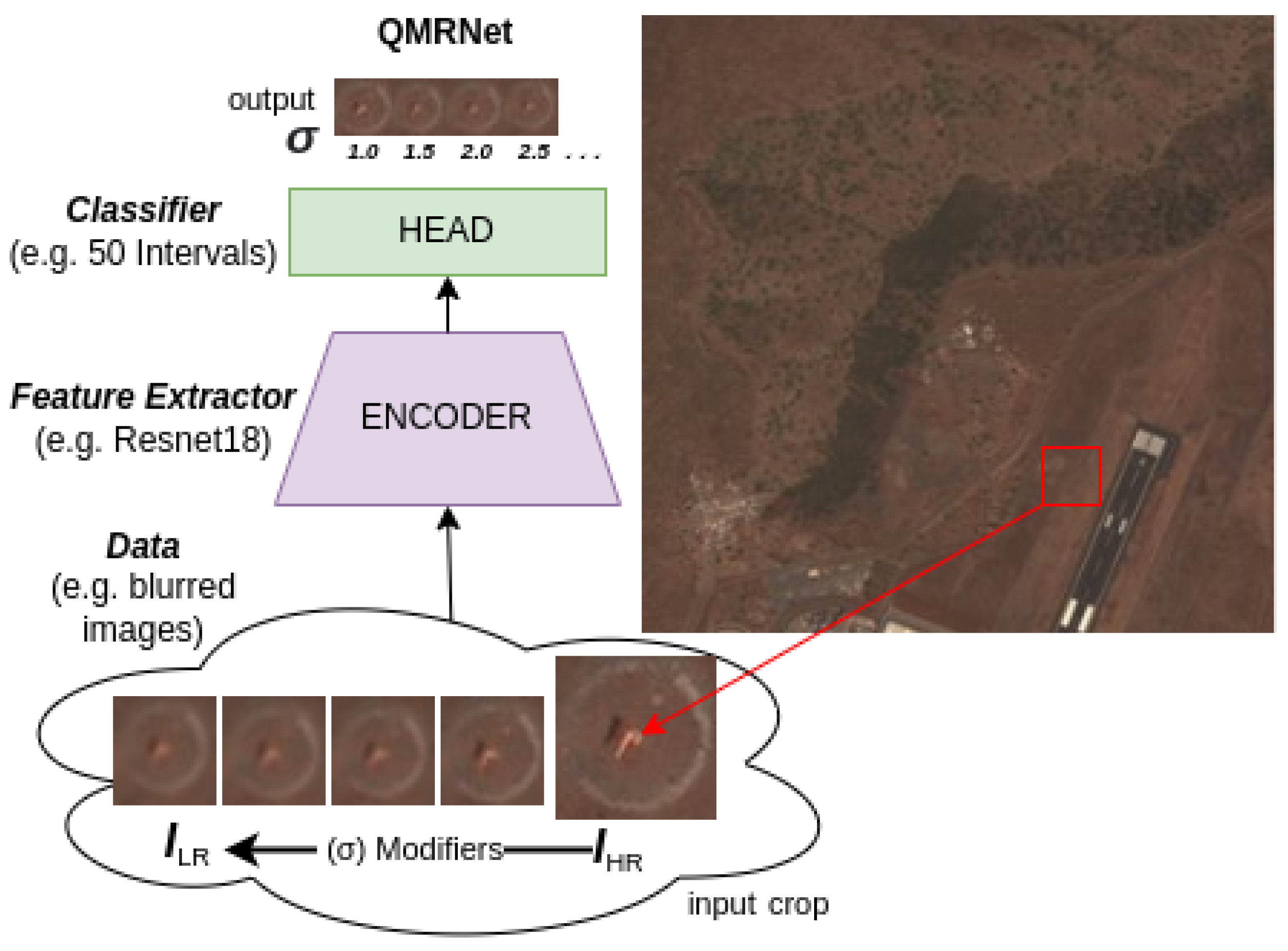
QMRNet is a feed-forward neural network that takes the architecture of an encoder with a parametrizable classifier (see Figure 1) upon numerical class intervals (can be set as binary, categorical or continuous according to the N intervals). It trains upon the predicted interval differences and the annotated parameters of the ground truth (GT) and requires a HEAD for each parameter to predict. In Figure 2 we designed 2 mechanisms of assessing the quality from several parameters simultaneously (multiparameter prediction): multibranch (MB) and multihead (MH). For MB a single encoder and head is required for each parameter to predict, while MH requires a head for each parameter but only one encoder. Therefore, QMRNet-MH considers one encoder and #N classifiers per EO parameter while QMRNet-MB considers #N encoders + #N classifiers (a whole QMRNet per parameter). The QMRNet-MH predicts all parameters simultaneously (faster) but its capacity is lower (can lead to lower accuracy) from the encoder part.
For our experiments with QMRNet we have used an encoder based on ResNet18 (backbone) composed of a convolutional layer (3 × 3) and 4 residual blocks (each composed of 4 convolutional layers) of 64, 128, 256 and 512 pixels of resolution. Our network is scalable to distinct crop resolutions as well as regression parameters (N intervals), adapting the HEAD to the number of classes to predict. The output of the HEAD after pooling is a continuous value of probability of each class interval, and through softmax and thresholding we can filter (one-hot) which class or classes have been predicted (1) and not (0) for each image sample crop. By default, we utilize the Binary Cross Entropy Loss (BCELoss) as the classification error and Stochastic Gradient Descend as the optimizer. For the case of multiclass regression, we designed the multibranch QMRNet (QMRNet-MB), in which we train each network individually with its set of parameterized modification intervals for each sample. QMRNet-MB is trained individually but can be run once per sample (parallel threads per branch), especially to obtain fast multi-class metric calculations (see s c o r e in Section 4.1).
Note that for processing irregular or inequivalent crops in our design of the network input, in the case of having the encoder input resolution R lower than the input image crops (e.g., 5000 × 5000 for GT and 256 × 256 for the network input), we crop the image to the QMRNet input R by C crops. C is the number of crops to generate for each sample (e.g., 10, 20, 50, 100, 200). In the case of the crops being smaller than the encoder backbone input (e.g., 232 × 232 for the GT and 256 × 256 for the network input), we apply a circular padding on each border (width and/or height) to obtain a real image that preserves the scaling and domain. The total number of hyperparameters to specify the design of a specific QMRNet architecture is N × R and it can be trained with a distinct combination of hyperparameters (N × C × R). To train the QMRNet’s regressor, we select a training set and generate a set of distorted cases, which are parameterizable through our modifiers. The total number of training samples (dataset size) can be calculated by the product of the dataset images (I) and N × C (number of parameter intervals and crops per sample). We can set distinct possible hyperparameters specifically to train and validate, such as the number of epochs (e), batch size (bs), learning rate (lr), weight decay (wd), momentum, soft thresholding, etc.

3.3. QMRLoss: Learning Quality Metric Regression as Loss in SR

We designed a novel objective function that is able to optimize super-resolution algorithms upon a specific quality objective using QMRNet (see Figure 3). Given a GAN or autoencoder network, we can add an ad hoc module based on a specific (or several) parameters of QMRNet. The QMRLoss is obtained by computing the classification error between the I S R prediction and the original I H R . This classification error determines whether the SR image is distinct in terms of a quality parameter objective (i.e., b l u r   σ , F, GSD, r e r or s n r ) with respect the HR. The QMRLoss has been designed to use any classification error (i.e., BCE, L1 or L2) and can be summated to the perceptual or content loss of the generator (decoder for autoencoders) in order to tune the SR to the quality objective.
The objective function for image generation algorithms is based on minimizing the generator (G) error (which compares I H R and I S R ) while maximizing the discriminator (D) error (which tests whether the SR image is true or fake).
min G max D = E H R l o g ( D ( I H R ) + E L R l o g ( 1 D ( I S R )
During training, G is optimized upon L S R , which considers L G P e r c and L A d v . We added a new term, L G Q M R , which will be our loss function based on the quality objectives (QMRNet). Note that here we consider I S R as the prediction image G ( I L R ) .
L S R = L G P e r c + L D A d v + L G Q M R λ Q M R
L D A d v = l o g D ( I S R )
L G P e r c = 1 n ( I H R I S R ) { 1 , 2 }
Below, we define the term L Q M R , which calculates the parameter difference between the I H R images and I S R images, regularized by the constant λ Q M R . This is performed by computing the classification error (L1, L2 or BCE) between the output of the heads for each case:
L L 1 Q M R = 1 n ( Q M R N e t ( I H R ) Q M R N e t ( I S R ) ) L L 2 Q M R = 1 n ( Q M R N e t ( I H R ) Q M R N e t ( I S R ) ) 2 L B C E Q M R = 1 n Q M R N e t ( I H R ) l o g ( Q M R N e t ( I S R ) ) + ( 1 Q M R N e t ( I H R ) ) l o g ( 1 Q M R N e t ( I S R ) )

4. Experiments

4.1. Experimental Setup

For training the QMRNet we collected 30cm/pixel data from the Inria Aerial Image Labeling Dataset (both training and validation using Inria-AILD sets). For testing our network, we selected all 11 subsets from the distinct EO datasets, USGS, UCMerced, Inria, DeepGlobe, Shipsnet, ECODSE and Xview (see Table 1).

4.1.1. Evaluation Metrics

In order to validate the training regime, we set several evaluation metrics (Table 4, Table 5 and Table 6) that provide interval dependencies for each prediction, namely, that intervals that are closer to the target interval are considered better predictions that further ones. This means that given an unblurred image ( b l u r   σ = 1.0 ) the prediction of σ = 2.5 will be a worse prediction than predictions closer to the GT (e.g., σ = 1.03 , σ = 1.2 ). For this, we considered retrieval metrics (which are N-rank order classification) such as medR or recall rate K (R@K) [49,50] as well as performance statistics (precision, recall, accuracy, F-score) at different intervals close to the target (Precision@K, Recall@K, Accuracy@K, F-Score@K) and overall Area Under ROC (AUC). The retrieval metric medR measures the median absolute interval difference between classes, namely, that for 10 classes and modifier GSD (30, 33 . 3 , 36 . 6 ,…, 60), if the targets (modified) are 33 . 3 and predictions are 36 . 6 then there is a medR of 1.0, while if predictions are 60 then medR is 9.0. R@K measures the total recall (whether prediction in an interval distance from the target is lower than K) over a target window (i.e., if there are 40 classes and K is 10, only the 10 classes around the target label are considered for evaluation).
In Table 7, Table 8 and Table 11 we add another quality metric in addition to the modifier-based ones, which is the s c o r e . For this s c o r e we defined a basis that describes the overall quality ranking (set from 0.0 to 1.0) of an image or dataset. This is calculated by measuring the weighted mean of the metrics, each metric with its own objective target (min↓ or max↑) as described in Table 2.
M s c o r e = M r a n g e | ( M o b j e c t i v e M p r e d i c t i o n ) M r a n g e
s c o r e = m = 1 m = 5 ω M m M s c o r e m
For a specific quality metric we define the total M r a n g e of the metric (i.e., for σ it would be 2.5 1.0 , namely, 1.5 ), an objective M o b j e c t i v e value (i.e., for σ it would be the minimum, as best the Q u a l i t y goes toward minimizing σ , namely, 1.0) and the weights ω M for the total weighted sum of the S c o r e (by default if we keep the same importance for each metric, ω M = 1 b , where m is the total number of modifiers, for our case m = 5 ).

4.1.2. Training and Validation

We trained our network with Inria-AILD sets of 180 images each for the training, validation and test subsets (Inria-AILD-180-train, Inria-AILD-180-val Inria-AILD-180-test, respectively), selecting 100 images for training and 20 for validation (proportional to 45% and 12% of the total, respectively). We processed all samples of the dataset with distinct intervals for each modifier (thus, we annotated each sample with that modification interval) and built our network with distinct heads: N σ = 50 , N F = 9 , N G S D = 10 , N r e r = 40 , N s n r = 40 . We selected a distinct set of crops for each resolution (C × R), in this case 10 crops of 1024 × 1024, 20 crops of 512 × 512, 50 crops of 256 × 256, 100 crops of 128 × 128 and 200 crops of 64 × 64. Thus, we generated datasets with different input resolutions but adapting the total domain capacity. The total number of trained images becomes 180x N 50 , 9 , 10 , 40 , 40 x C 10 , 20 , 50 , 100 , 200 (e.g., a b l u r   σ 64 × 64 image set contains 1.8M crop samples).
We ran our training and validation experiments for 200 epochs with distinct hyperparameters: l r = [ 10 2 , 10 3 , 10 4 , 10 5 ], w d = [ 10 3 , 10 4 , 10 5 ], momentum = 0.9 and soft threshold 0.3 (to filter out soft to hard/one-hot labels). Due to the computational capacity, the training batch sizes were selected according to the resolution for each set: b s R = 64 × 64 , 128 × 128 = [ 32 , 64 , 128 , 256 ] , b s R = 256 × 256 = [ 16 , 32 , 64 , 128 ] , b s R = 512 × 512 = [ 8 , 16 , 32 , 64 ] and b s R = 1024 × 1024 = [ 4 , 8 , 16 , 32 ] .
In Table 4 we show the validation results (Inria-AILD-180-test) with the trained QMRNet using a ResNet18 backbone with the Inria-AILD-180-train data. We can observe that the overall medRs are around 1.0 (predictions are about one interval of distance with respect to the targets) and recall rates (exact match) are for top-1 (R@1) around 70% and for R@5 and R@10 (prediction is in an interval below 5 and 10 of the distance with respect to the target, respectively) around 100%. This means our network is able to predict the parameter data ( b l u r   σ , sharpness F, GSD, s n r , r e r ) with a very high retrieval precision, even when the parameters are fine-grained (e.g., 40 or 50 class intervals). The best results appear for low N parameters (smaller classification tasks), such as F and GSD. Here, GSD is mostly an easy task, as the scaling of objects is constant whether the images are distorted or not. In terms of the crop size, the best results are mostly in a higher input resolution of networks ( R = 1024 × 1024 ); this may vary on the selected backbone for the encoder (here, Resnet18 is mostly used with input R around 256 × 256 ).
In Table 5 are shown the validation results for multiparameter prediction, in which we tested multibranch QMRNet (QMRNet-MB) and multihead QMRNet (QMRNet-MH). Here, the performance between the two is similar to the single-parameter prediction (Table 4), where medR is around 1.0 and the recall rates around 70% for R@1 and >90% for R@5 and R@10. We tested predictions for two simultaneous parameters ( b l u r + r e r , F + G S D and s n r + r e r ) and overall QMRNet-MB obtains better results for b l u r + r e r and s n r + r e r but slightly worse for F + G S D than QMRNet-MH.
In Table 6 are shown the validation results for QMRNet’s prediction of s n r and r e r in hyperspectral images (ECODSE RSData with 426 bands per pixel). By changing the first convolutional layer of QMRNet’s encoder backbone for multiband input channels we can classify the quality metric with multichannel and hyperspectral images. Overall, medR is around 5.0 and the recall rates around 20% for R@1 (exact match), 56% for R@5 (five closest categories) and 80% for R@10 (ten closest categories). Here, the precision is lower due to the hardness of the approximation task, given the hyperspectral resolution (i.e., 80 × 80 at 60 cm/px) and the very few examples (43 examples). Despite the hardness of the dataset task, QMRNet with ResNet18 is able measure whether a parameter is in a specific range of s n r or r e r in hyperspectral images.
In Figure 4 we can see that most of the worst predictions for blur, sharpness, rer and snr appear mainly when attempting to predict over crops with sparse or homogeneous features, namely, when most of the image has limited or little pixel information (i.e., with similar pixel values), such as the sea or flat terrain surfaces. This is because the preprocessed samples have few or no dissimilarities in each modifier parameter. This has an effect on evaluating the datasets: when the surfaces are more sparse, predictions become harder.

4.2. Results on QMRNet for IQA: Benchmarking Image Datasets

We ran our QMRNet with a ResNet18 backbone over the sets (See the EO dataset evaluation use case in https://github.com/dberga/iquaflow-qmr-eo, accessed on 10 October 2022) described in Table 1. Given our network trained uniquely on Inria-AILD-180-train, we see how our network is able to adapt due to the prediction of feasible quality metrics ( b l u r   σ , GSD, sharpness F, s n r and r e r ) over each of the distinct datasets. We see that with fine-tuning QMRNet over Inria-AILD-180-train, the overall σ for most of the datasets appears to be σ = 1.0 (originally unblurred from the ground truth) except for USGS279 and Inria-AILD-180-test, which is around σ = 1.02 . For the case of the sharpness factor F, the overall values for most datasets is F = 1.0 (without oversharpening) but for cases such as UCMerced380 and Shipnset, it appears to be oversharpened ( F > 1.5 and F > 3.0 , respectively). Most datasets present an overall predicted s n r of M ( s n r ) = 28.67 and r e r of M ( r e r ) = 0.4896 . The highest S c o r e datasets are Inria-AILD-180-train, UCMerced2100 and USGS279, here considering the same weight ω M for each modifier metric M.

4.3. Results on QMRNet for IQA: Benchmarking Image Super-Resolution

Here we selected a set of super-resolution algorithms that have been previously tested to super-resolve high-quality real-image SR dataset benchmarks such as BSD100, Urban100 or Set5 × 2 (https://paperswithcode.com/task/image-super-resolution, accessed on 10 October 2022) but here we want to apply them to EO data and metrics. For this we want to benchmark their performance considering full-reference, no-reference and our QMRNet-based metric (See the use case of super-resolution benchmark at https://github.com/dberga/iquaflow-qmr-sisr, accessed on 10 October 2022). QMRNet allows us to check the amount of each distortion for every transformation (LR) applied to the original image (HR), if it is either the usual x2, x3 or x4 downsampling or a specific distortion such as blurring.
Concretely, we tested our UCMerced subset of 380 images with crops of 256 × 256 with autoencoder algorithms (FSRCNN and MSRN) and GAN-based and self-supervised architectures such as SRGAN, ESRGAN, CAR and LIIF. All model checkpoints are selected as vanilla (default hyperparameter settings) except for the input scaling (x2, x3, x4) and also for the case of MSRN, for which we computed three versions of the vanilla MSRN (architecture with four scales), one without fine-tuning ( M S R N 1 ), one with fine-tuning and added noise ( M S R N 2 ) and one ( M S R N 3 ) with fine-tuning (over Inria-AILD-180-train).
In Table 8 we have evaluated each type of modifier parameter for every single super-resolution algorithm as well as the overall score for all quality metric regression. Here, we tested the algorithms considering x2, x3 and x4 downsampling input (LR x 2 , x 3 , x 4 ), as well as considering the case of adding a blur filter with a scaled σ . Here, the QMRNet is able to predict that I L R gives the worst ranking for most metrics. FSRCNN and SRGAN give similar results in most metrics, with SRGAN being slightly better in the b l u r and s n r metrics. MSRN shows the best results in s n r and F, mainly when the inputs have a higher resolution (i.e., x2, x3). For the overall scores, CAR presents the best results in b l u r and r e r , with the highest score ranking in most downsampling cases. However, CAR has the worst ranking in the noise and sharpness metrics ( s n r and F). As we mentioned earlier, CAR presents oversharpening and hallucinations, which can trick some metrics that measure blur but becomes worse for those that predict unusual signal-to-noise ratios and illusory edges. In contrast, LIIF presents a bad performance in the b l u r and r e r metrics (meaning LIIF’s I S R images appearing slightly blurred), although LIIF acquires a overall good performance for the rest of the modifier metrics. We want to pinpoint that in some metrics (i.e., s n r , r e r and F), some of the tested algorithms (Table 8, Table 9 and Table 10) show lower distortion values than the original I H R . This phenomenon means that our metrics can demonstrate if an image has a present distortion effect (whether it is oversharpening, blur or noise) beyond its image quality, unlike full-reference metrics, which are limited to the quality of the I H R samples.
In Table 9 we show a benchmark of known full-reference metrics. In super-resolving x2, MSRN (concretely, M S R N 2 and M S R N 3 ) has the best results for full-reference metrics, including SSIM, PSNR, SWD, FID, MSSIM, HAARPSI and MDSI. In x3 and x4, LIIF and CAR have the best results for most of these metrics, including PSNR, FID, GMSD and MDSI, being top-3 with most metric evaluations. Here we have to pinpoint that LIIF does not perform as well when the input ( I L R ) has been blurred; see here that CAR is able to deblur the input better than other algorithms as it is oversharpening the originally downscaled and/or blurred I L R . In Table 10 we show the no-reference metric results, here for SNR, RER, MTF and FWHM. SRGAN, MSRN and LIIF present significantly better results for SNR than other algorithms. This means these algorithms in general do not add noise to the input, namely, the generated images do not contain artifacts that were not present in the original I H R . In this case, CAR outperforms in RER, MTF and FWHM.
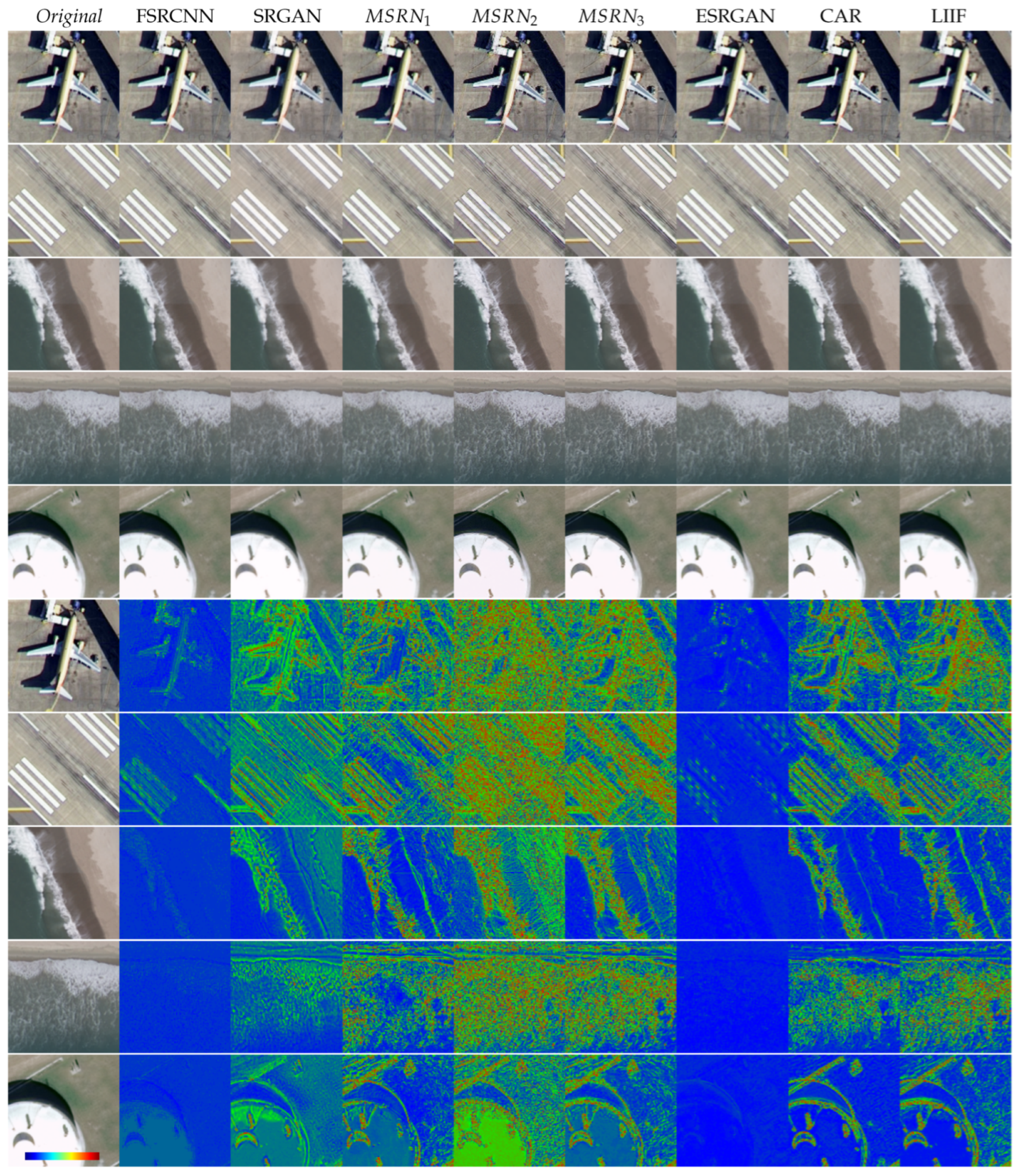
In Figure 5 and Figure 6 we super-resolve the original UCMerced and XView images x3 and we can observe that some algorithms, such as FSRCNN, SRGAN, M S R N 1 , ESRGAN and LIIF, present a similar (blurred) output, while others, such as M S R N 2 , M S R N 3 and CAR, present a higher noise and oversharpening of borders, trying to enhance the features of the image (here, attempting to generate features beyond the I L R content). The noise and oversharpening are distinguishable in colormaps of buildings (e.g., Figure 5, row 10 and Figure 7, row 6).
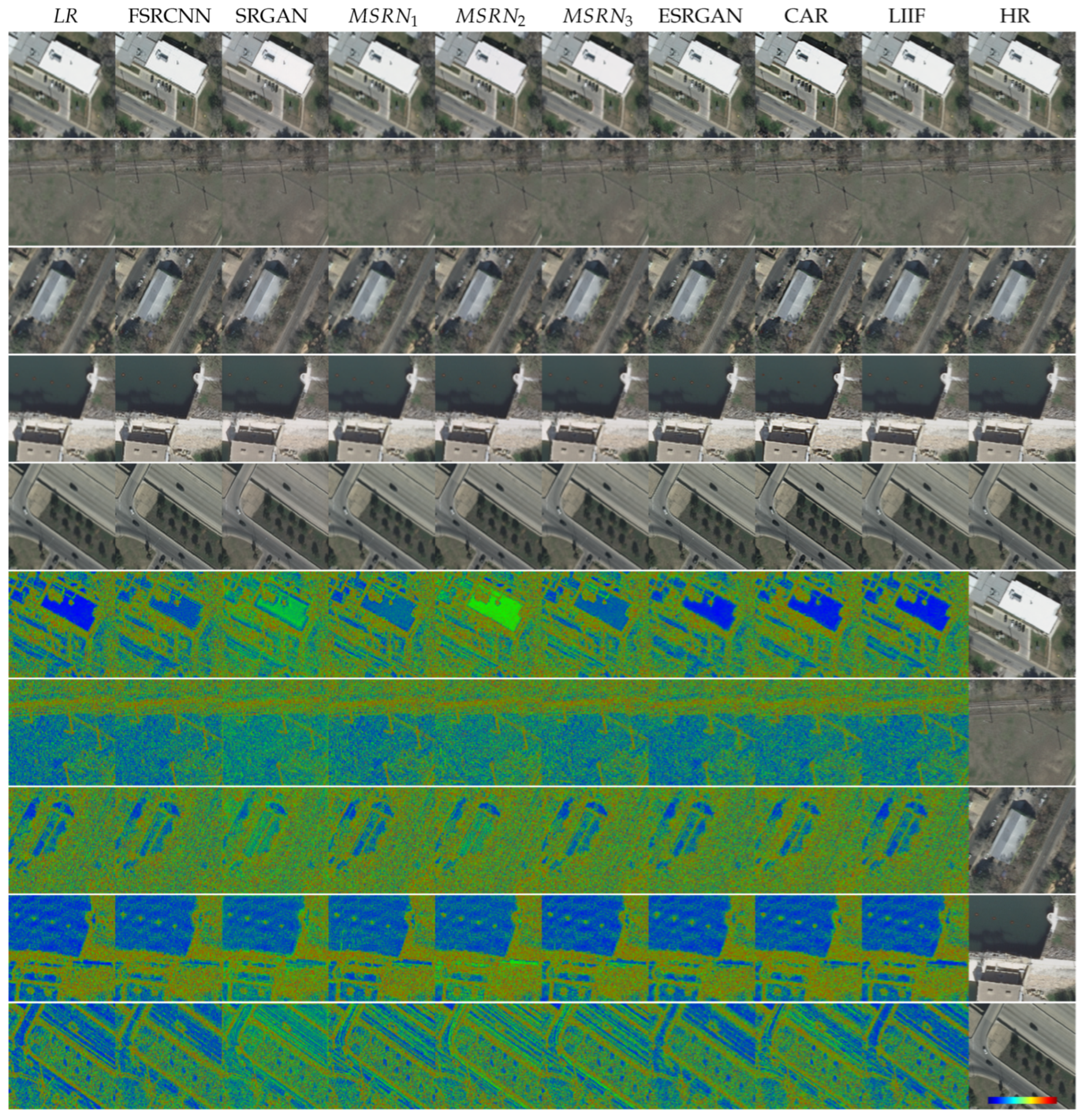
In our results for low-resolution LR x 3 inputs we can qualitatively see (Figure 7) that FSRCNN, SRGAN, M S R N 1 and LIIF present blurred outputs, similar to the I L R . ESRGAN does not change much the appearance with respect to the original image (see differences in colormaps), but simply adds some residual noise at the edges. CAR, however, seems to acquire better results but it appears in some cases to be oversharpened (similar to MSRN 3 ). We can observe that MSRN algorithms do not perform well when super-resolving very-low-resolution images (i.e., the downsampled I L R ). Its original training set might not have considered very-low-resolution image samples. See Section 4.4 for MSRN optimization using QMRNet.
Above (Figure 8) we demonstrate the validity of some of our metric results by comparing them with each homologous measurement, namely, the ones measuring similar or the same properties. Here, we compared QMRNet’s s n r and PSNR↑. These measure the quantity of noise over information of the image. The first subplot shows an anticorrelation (↙) on the algorithm values in these two metrics, with LIIF being closest to the I H R (GT) and CAR, M S R N 2 and M S R N 3 having both the lowest s n r (best) and PSNR (worst). For the case of QMRNet’s r e r and measured R E R o t h e r (which corresponds to the RER that measures diagonal contours), there is a positive correlation (↗), with CAR, M S R N 2 and M S R N 3 outperforming the rest of the algorithms. We also compared F W H M o t h e r and SSIM↑ to see how well each algorithm performs when evaluating the diagonal contour width as well as the structural similarity, and it appears that M S R N 2 , M S R N 3 and CAR have the lowest (best) F W H M and most algorithms have the same values of SSIM as the original GT images (unchanged). In the last subplot we compared the QMRNet’s s c o r e (composed of the weighted mean of QMRNet’s s i g m a , r e r , s n r , G S D and F) and FID↓, which measures the Fréchet distribution distance between images. Here M S R N 2 , M S R N 3 and CAR show the highest s c o r e with higher (worse) FID, while most algorithms are close to the original image (almost unchanged). Note that in these plots we super-resolve x4 the original image so that full-reference metrics can only compare with the original image (thus, there is no downsampling of inputs so that the I H R would be equivalent to the I L R input). Here, we need to consider how the algorithms actually perform in metrics that can evaluate better than the original image.

4.4. Results on QMRloss: Optimizing Image Super-Resolution

In this section, we integrated the aforementioned QMRLoss as an ad-hoc regularization strategy for optimizing SR algorithms (See the QMRLoss optimization use case at https://github.com/dberga/iquaflow-qmr-loss, accessed on 10 October 2022). For this case, we integrated different loss methods (L1, L2 and BCE) as QMRLoss in different modifiers in MSRN training. We regularized the MSRN architecture by integrating the QMRLoss ( L Q M R ) to the total loss calculation, namely, summed to the adversarial loss L a d v and the perceptual loss L p e r c (in this case, VGGLoss). This QMRLoss regularization mechanism will allow MSRN and any other algorithm to avoid quality mismatches considering several metrics that measure distortions simultaneously (see results in Table 11).
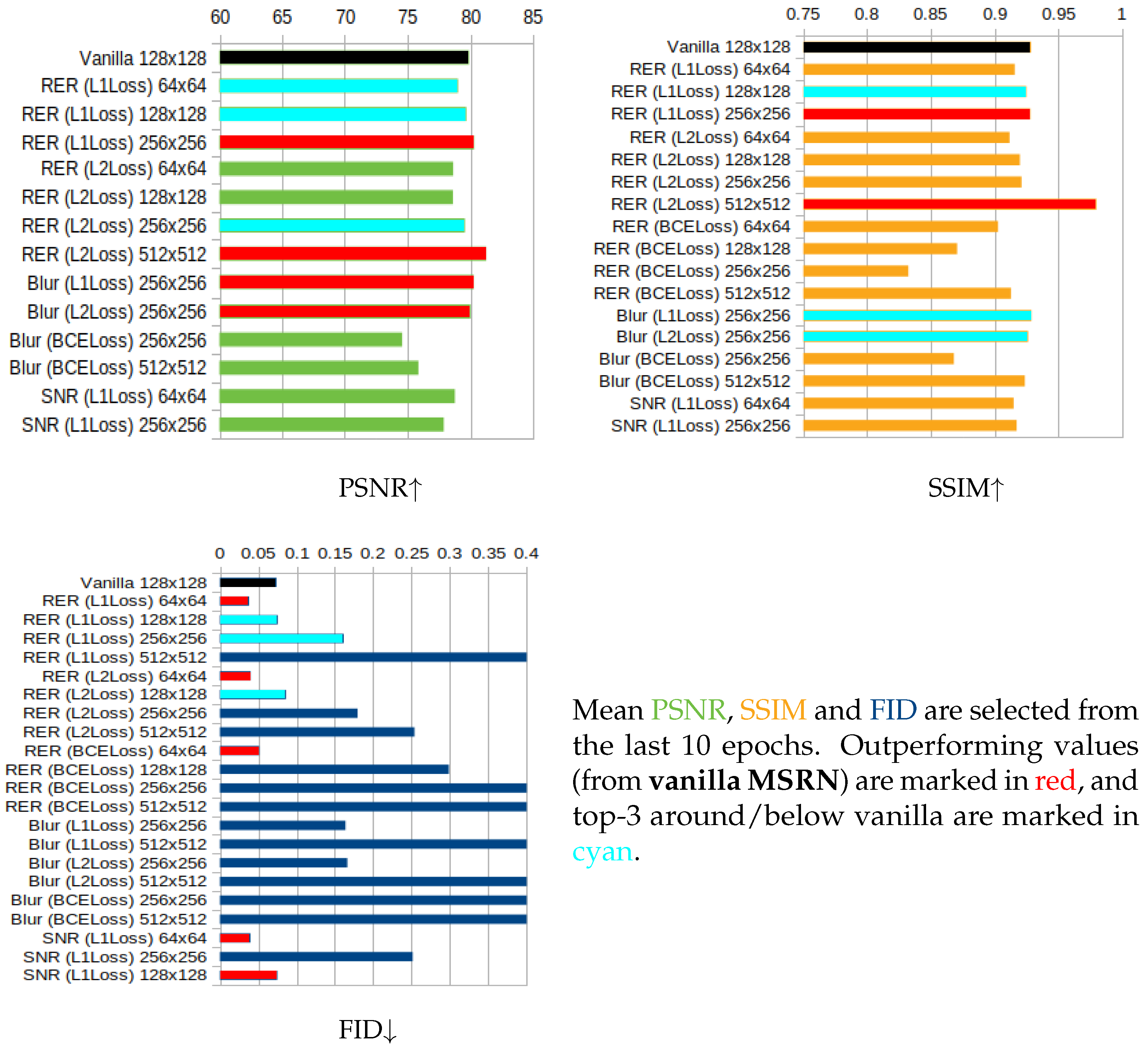
In Figure 9 we show that several strategies such as QMRLoss using r e r (and L1 loss) obtain better results than vanilla MSRN in the PSNR, SSIM and FID metrics. Here, the PSNR improves with QMRNet using L1 loss and crops of 256 × 256 as well as with L2 loss with 512 × 512. It also improves with the b l u r metric both with L1 and L2 loss on 256 × 256 crops. The SSIM improves with L1 loss in QMRNet that uses RER and significatively (almost 1.0) with r e r L2 loss with crops of 512 × 512. For FID, using QMRNet improves MSRN with r e r and all types of losses (L1, L2 and BCE) using crops of 64 × 64, here as well using QMRNet with s n r metric and L1 loss, using crops of 64 × 64 and 128 × 128.
We also tested our MSRN + QMRLoss (adding QMRNet’s metric evaluation) generated images with most of our full-reference and no-reference metrics in the UCMerced-380 dataset (outside Inria-AILD’s training and validation distribution) with crops of 256 × 256. Here, vanilla MSRN yields worse results for b l u r , s n r , r e r , SNR M d n , RER mean of X and Y ↑, MTF mean of X and Y ↑ and FWHM mean of X and Y ↓ in comparison with the optimized QMRLoss σ , L 1 , 256 × 256 , QMRLoss r e r , L 1 , 256 × 256 and QMRLoss F , L 1 , 256 × 256 . Here, QMRLoss L 1 has been able to adapt better when generating contours and predicting blurred objects on testing distinct shapes from the original training. In the case of full-reference metrics, I L R is more similar to the original I H R (although seemingly blurred); this is due to the lack of changes made to the image. In the no-reference metrics, MSRN+QMR significatively improves with respect to I L R and MSRN v a n i l l a .
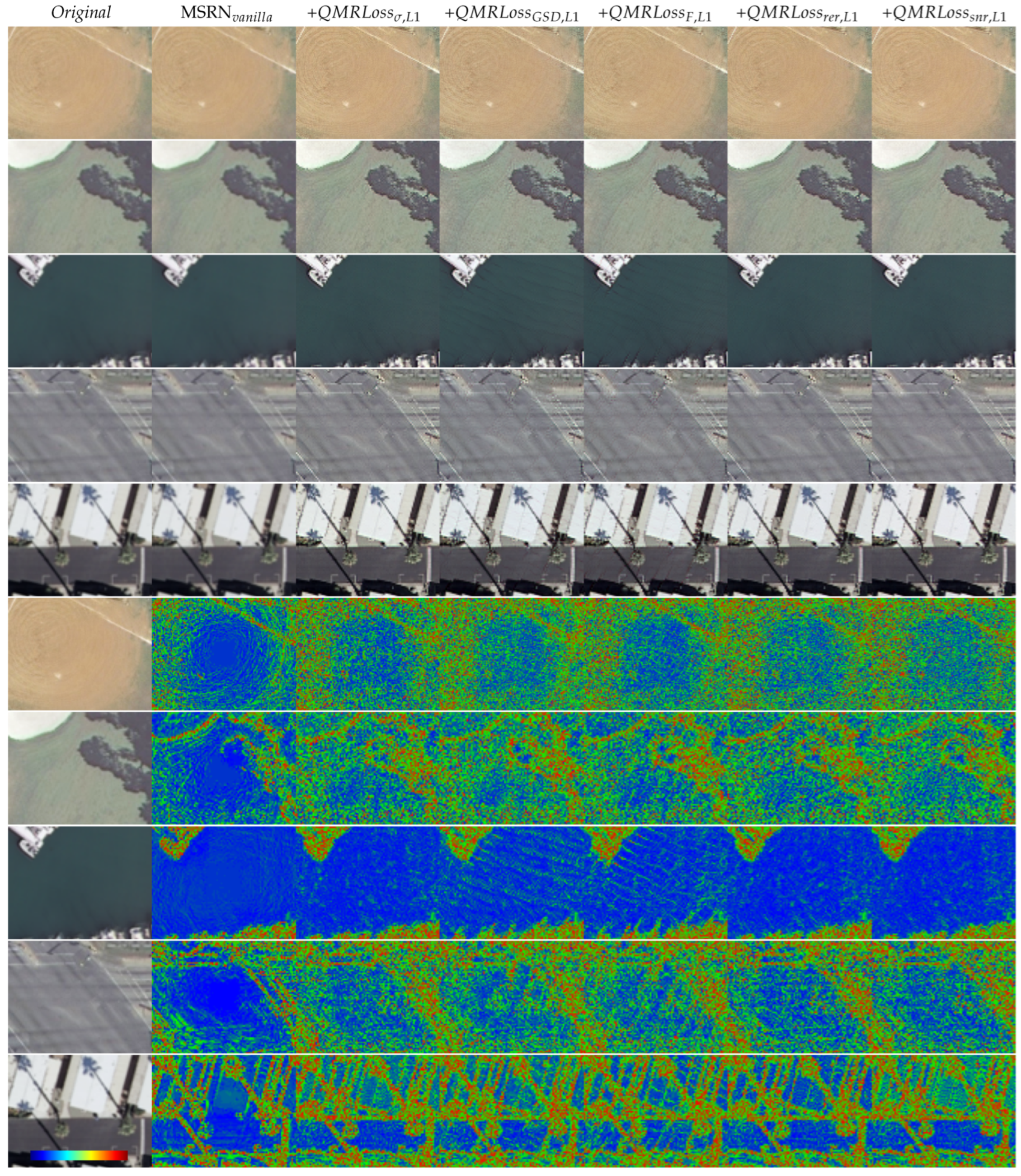
In Figure 10, Figure 11 and Figure 12 can be observed the changes of super-resolving UCMerced and Inria-AILD images according to every QMRNet optimization. In most cases of MSRN v a n i l l a (column 2 colormaps) there is a center bias, especially in sparse/homogeneous regions. In Figure 11, row 3 and Figure 12, row 1 it can be observed that QMRLoss G S D , L 1 and QMRLoss F , L 1 significatively enhance the noise present in the homogeneous areas (sea/beach), while QMRLoss σ , L 1 , QMRLoss r e r , L 1 and QMRLoss s n r , L 1 present a smoother solution whilst having higher oversharpening than MSRN v a n i l l a .

5. Conclusions

In this study, we implement an open-source tool (integrated in the IQUAFLOW framework) developed for assessing quality and modifying EO images. We propose a network architecture (QMRNet) that predicts the amount of distortion for each parameter as a no-reference metric. We also benchmark distinct super-resolution algorithms and datasets with both full-reference and no-reference metrics and propose a novel mechanism for optimizing super-resolution training regimes using QMRLoss, integrating QMRNet metrics with SR algorithm objectives. We tested the performance in single-parameter prediction of b l u r , r e r , s n r , F and GSD, as well as multiparameter simultaneously. In addition to the high-resolution color EO image computation, we adapted and tested the QMRNet architecture for the prediction of s n r and r e r with hyperspectral EO images.
On assessing the image quality of datasets we observe similar overall scores for most datasets, with dissimilarities in the scores of s n r and r e r . On assessing the single-image super-resolution we see significantly better results for CAR, LIIF, M S R N 2 and M S R N 3 . Optimizing MSRN with QMRLoss (snr, rer and blur) improves the results on both full-reference and no-reference metrics with respect to the default vanilla MSRN.
We have to point out that our proposed method can be applied to any type of distortion or modification. QMRNet allows us to predict any parameter of the image and also several parameters simultaneously. For instance, training QMRNet to assess compression parameters could be another use case of interest, including other datasets mentioned in Section 2. We also tested the usage of QMRNet as loss for optimizing SR results by regularizing the MSRN network, but it could be extended with distinct algorithm architectures and uses, as QMRLoss allows us to reverse or denoise any modification of the original image. In addition, it is also possible to implement a variation to the QMRLoss objective by forcing the loss calculation to be on a specific interval with maximum quality and minimal distortion for each parameter. In that way, the algorithm could maximize toward a specific metric or s c o r e objective beyond the output over the GT.

Author Contributions

Conceptualization, D.B., D.V. and J.M.; methodology, D.B.; software, D.B., P.G., L.R.-C., K.T., C.G.-M. and E.M.; validation, D.B.; formal analysis, D.B.; investigation, D.B. and J.M.; resources, D.B. and J.M.; data curation, D.B.; writing—original draft, D.B.; writing—review and editing, D.B., P.G. and J.M.; visualization, D.B.; supervision, D.B., J.M., P.G. and D.V.; project administration, D.B., J.M. and D.V.; funding acquisition, D.B., J.M. and D.V. All authors have read and agreed to the published version of the manuscript.

Funding

The project was financed by the Ministry of Science and Innovation (MICINN) and by the European Union within the framework of FEDER RETOS-Collaboration of the State Program of Research (RTC2019-007434-7), Development and Innovation Oriented to the Challenges of Society, within the State Research Plan Scientific and Technical and Innovation 2017–2020, with the main objective of promoting technological development, innovation and quality research.

Data Availability Statement

The research code and data are specified in the following repositories:

Conflicts of Interest

The authors declare that they have no known competing financial interests nor personal relationships that could have appeared to influence the work reported in this paper.

Abbreviations

The following abbreviations are used in this manuscript:
SR| I S R Super-Resolution|SR image
HR| I H R High-Resolution|HR image
LR| I L R Low-Resolution|LR image
EOEarth Observation
IQAImage Quality Assessment
GSDGround Sampling Distance
GANGenerative Adversarial Networks
SNRSignal-to-Noise
RERRelative Edge Response
MTFModulation Transfer Function
LSFLine Spread Function
PSFPoint Sparsity Function
FWHMFull Width at Half Maximum
PSNRPeak Signal-to-Noise Ratio
SSIMStructural Similarity
MSSIMMean Structural Similarity
HAARPSIHaar Wavelet Perceptual Similarity Index
GMSDGradient Magnitude Similarity Deviation
MDSIMean Deviation Similarity Index
SWDSliced Wasserstein Distance
FIDFréchet Inception Distance

References

  1. Leachtenauer, J.C.; Driggers, R.G. Surveillance and Reconnaissance Imaging Systems: Modeling and Performance Prediction; Artech House Optoelectronics Library: Norwood, MA, USA, 2001. [Google Scholar]
  2. Dong, C.; Loy, C.C.; He, K.; Tang, X. Image Super-Resolution Using Deep Convolutional Networks. IEEE Trans. Pattern Anal. Mach. Intell. 2016, 38, 295–307. [Google Scholar] [CrossRef]
  3. Yamanaka, J.; Kuwashima, S.; Kurita, T. Fast and Accurate Image Super Resolution by Deep CNN with Skip Connection and Network in Network. In Neural Information Processing; Springer International Publishing: Long Beach, CA, USA, 2017; pp. 217–225. [Google Scholar] [CrossRef]
  4. Müller, M.U.; Ekhtiari, N.; Almeida, R.M.; Rieke, C. Super-resolution of multispectral satellite images using convolutional neural networks. arXiv 2020, arXiv:2002.00580. [Google Scholar] [CrossRef]
  5. Li, J.; Fang, F.; Mei, K.; Zhang, G. Multi-scale Residual Network for Image Super-Resolution. In Proceedings of the European Conference on Computer Vision (ECCV); Springer International Publishing: Munich, Germany, 2018; pp. 527–542. [Google Scholar] [CrossRef]
  6. Ledig, C.; Theis, L.; Huszar, F.; Caballero, J.; Cunningham, A.; Acosta, A.; Aitken, A.; Tejani, A.; Totz, J.; Wang, Z.; et al. Photo-Realistic Single Image Super-Resolution Using a Generative Adversarial Network. In Proceedings of the 2017 IEEE Conference on Computer Vision and Pattern Recognition (CVPR), Honolulu, HI, USA, 21–26 July 2017. [Google Scholar] [CrossRef]
  7. Wang, X.; Yu, K.; Wu, S.; Gu, J.; Liu, Y.; Dong, C.; Qiao, Y.; Loy, C.C. ESRGAN: Enhanced Super-Resolution Generative Adversarial Networks. In Workshop of the European Conference on Computer Vision (ECCV); Springer International Publishing: Munich, Germany, 2019; pp. 63–79. [Google Scholar] [CrossRef]
  8. Jiang, Y.; Gong, X.; Liu, D.; Cheng, Y.; Fang, C.; Shen, X.; Yang, J.; Zhou, P.; Wang, Z. EnlightenGAN: Deep Light Enhancement Without Paired Supervision. IEEE Trans. Image Process. 2021, 30, 2340–2349. [Google Scholar] [CrossRef] [PubMed]
  9. Kim, J.; Lee, J.K.; Lee, K.M. Accurate Image Super-Resolution Using Very Deep Convolutional Networks. In Proceedings of the IEEE Conference on Computer Vision and Pattern Recognition (CVPR Oral), Las Vegas, NV, USA, 27–30 June 2016. [Google Scholar]
  10. Sun, W.; Chen, Z. Learned image downscaling for upscaling using content adaptive resampler. IEEE Trans. Image Process. 2020, 29, 4027–4040. [Google Scholar] [CrossRef] [PubMed]
  11. Chen, Y.; Liu, S.; Wang, X. Learning Continuous Image Representation with Local Implicit Image Function. arXiv 2020, arXiv:2012.09161. [Google Scholar]
  12. Pradham, P.; Younan, N.H.; King, R.L. Concepts of image fusion in remote sensing applications. In Image Fusion; Elsevier: Amsterdam, The Netherlands, 2008; pp. 393–428. [Google Scholar] [CrossRef]
  13. Huynh-Thu, Q.; Ghanbari, M. Scope of validity of PSNR in image/video quality assessment. Electron. Lett. 2008, 44, 800. [Google Scholar] [CrossRef]
  14. Wang, Z.; Bovik, A.; Sheikh, H.; Simoncelli, E. Image Quality Assessment: From Error Visibility to Structural Similarity. IEEE Trans. Image Process. 2004, 13, 600–612. [Google Scholar] [CrossRef] [PubMed]
  15. Reisenhofer, R.; Bosse, S.; Kutyniok, G.; Wiegand, T. A Haar wavelet-based perceptual similarity index for image quality assessment. Signal Process. Image Commun. 2018, 61, 33–43. [Google Scholar] [CrossRef]
  16. Xue, W.; Zhang, L.; Mou, X.; Bovik, A.C. Gradient Magnitude Similarity Deviation: A Highly Efficient Perceptual Image Quality Index. IEEE Trans. Image Process. 2014, 23, 684–695. [Google Scholar] [CrossRef]
  17. Nafchi, H.Z.; Shahkolaei, A.; Hedjam, R.; Cheriet, M. Mean Deviation Similarity Index: Efficient and Reliable Full-Reference Image Quality Evaluator. IEEE Access 2016, 4, 5579–5590. [Google Scholar] [CrossRef]
  18. Varga, D. Full-Reference Image Quality Assessment Based on an Optimal Linear Combination of Quality Measures Selected by Simulated Annealing. J. Imaging 2022, 8, 224. [Google Scholar] [CrossRef] [PubMed]
  19. Lim, P.C.; Kim, T.; Na, S.I.; Lee, K.D.; Ahn, H.Y.; Hong, J. Analysis of UAV image quality using edge analysis. Int. Arch. Photogramm. Remote. Sens. Spat. Inf. Sci. 2018, 42, 359–364. [Google Scholar] [CrossRef]
  20. Mittal, A.; Soundararajan, R.; Bovik, A.C. Making a “Completely Blind” Image Quality Analyzer. IEEE Signal Process. Lett. 2013, 20, 209–212. [Google Scholar] [CrossRef]
  21. Venkatanath, N.; Praneeth, D.; Bh, M.C.; Channappayya, S.S.; Medasani, S.S. Blind image quality evaluation using perception based features. In Proceedings of the 2015 Twenty First National Conference on Communications (NCC), Mumbai, India, 27 February–1 March 2015. [Google Scholar] [CrossRef]
  22. Leachtenauer, J.C.; Malila, W.; Irvine, J.; Colburn, L.; Salvaggio, N. General Image-Quality Equation: GIQE. Appl. Opt. 1997, 36, 8322. [Google Scholar] [CrossRef]
  23. Thurman, S.T.; Fienup, J.R. Analysis of the general image quality equation. In Visual Information Processing XVII; ur Rahman, Z., Reichenbach, S.E., Neifeld, M.A., Eds.; SPIE: Bellingham, WA, USA, 2008. [Google Scholar] [CrossRef]
  24. Kim, T.; Kim, H.; Kim, H.D. Image-based Estimation and Validation of Niirs for High-resolution Satellite Images. Int. Arch. Photogramm. Remote. Sens. Spat. Inf. Sci. 2008, 37, 1–4. [Google Scholar]
  25. Li, L.; Luo, H.; Zhu, H. Estimation of the Image Interpretability of ZY-3 Sensor Corrected Panchromatic Nadir Data. Remote Sens. 2014, 6, 4409–4429. [Google Scholar] [CrossRef]
  26. Benecki, P.; Kawulok, M.; Kostrzewa, D.; Skonieczny, L. Evaluating super-resolution reconstruction of satellite images. Acta Astronaut. 2018, 153, 15–25. [Google Scholar] [CrossRef]
  27. Johnson, J.; Alahi, A.; Fei-Fei, L. Perceptual Losses for Real-Time Style Transfer and Super-Resolution. In Computer Vision–ECCV 2016; Springer International Publishing: Amsterdam, The Netherlands, 2016; pp. 694–711. [Google Scholar] [CrossRef]
  28. Zhang, R.; Isola, P.; Efros, A.A.; Shechtman, E.; Wang, O. The Unreasonable Effectiveness of Deep Features as a Perceptual Metric. In Proceedings of the 2018 IEEE/CVF Conference on Computer Vision and Pattern Recognition, Salt Lake City, UT, USA, 18–22 June 2018. [Google Scholar] [CrossRef]
  29. Kolouri, S.; Nadjahi, K.; Simsekli, U.; Badeau, R.; Rohde, G. Generalized Sliced Wasserstein Distances. In Proceedings of the Advances in Neural Information Processing Systems; Wallach, H., Larochelle, H., Beygelzimer, A., d’Alché-Buc, F., Fox, E., Garnett, R., Eds.; Curran Associates, Inc.: Knoxville, TN, USA, 2019; Volume 32. [Google Scholar]
  30. Salimans, T.; Goodfellow, I.; Zaremba, W.; Cheung, V.; Radford, A.; Chen, X.; Chen, X. Improved Techniques for Training GANs. In Proceedings of the Advances in Neural Information Processing Systems; Lee, D., Sugiyama, M., Luxburg, U., Guyon, I., Garnett, R., Eds.; Curran Associates, Inc.: Knoxville, TN, USA, 2016; Volume 29. [Google Scholar]
  31. Liu, J.; Zhou, W.; Li, X.; Xu, J.; Chen, Z. LIQA: Lifelong Blind Image Quality Assessment. IEEE Trans. Multimed. 2022; Early Access. [Google Scholar] [CrossRef]
  32. Chen, L.H.; Bampis, C.G.; Li, Z.; Norkin, A.; Bovik, A.C. ProxIQA: A Proxy Approach to Perceptual Optimization of Learned Image Compression. IEEE Trans. Image Process. 2021, 30, 360–373. [Google Scholar] [CrossRef]
  33. Saad, M.A.; Bovik, A.C.; Charrier, C. Blind Image Quality Assessment: A Natural Scene Statistics Approach in the DCT Domain. IEEE Trans. Image Process. 2012, 21, 3339–3352. [Google Scholar] [CrossRef]
  34. Mittal, A.; Moorthy, A.K.; Bovik, A.C. No-reference image quality assessment in the spatial domain. IEEE Trans. Image Process. 2012, 21, 4695–4708. [Google Scholar] [CrossRef] [PubMed]
  35. Ye, P.; Kumar, J.; Kang, L.; Doermann, D. Unsupervised feature learning framework for no-reference image quality assessment. In Proceedings of the 2012 IEEE Conference on Computer Vision and Pattern Recognition, Providence, RI, USA, 16–21 June 2012; pp. 1098–1105. [Google Scholar] [CrossRef]
  36. Xu, J.; Ye, P.; Li, Q.; Du, H.; Liu, Y.; Doermann, D. Blind Image Quality Assessment Based on High Order Statistics Aggregation. IEEE Trans. Image Process. 2016, 25, 4444–4457. [Google Scholar] [CrossRef] [PubMed]
  37. Liu, X.; van de Weijer, J.; Bagdanov, A.D. RankIQA: Learning From Rankings for No-Reference Image Quality Assessment. In Proceedings of the IEEE International Conference on Computer Vision (ICCV), Venice, Italy, 22–29 October 2017. [Google Scholar]
  38. Bosse, S.; Maniry, D.; Muller, K.R.; Wiegand, T.; Samek, W. Deep Neural Networks for No-Reference and Full-Reference Image Quality Assessment. IEEE Trans. Image Process. 2018, 27, 206–219. [Google Scholar] [CrossRef]
  39. Fan, C.; Zhang, Y.; Feng, L.; Jiang, Q. No Reference Image Quality Assessment based on Multi-Expert Convolutional Neural Networks. IEEE Access 2018, 6, 8934–8943. [Google Scholar] [CrossRef]
  40. Zhu, H.; Li, L.; Wu, J.; Dong, W.; Shi, G. MetaIQA: Deep Meta-Learning for No-Reference Image Quality Assessment. In Proceedings of the Proceedings of the IEEE Conference on Computer Vision and Pattern Recognition (CVPR), Seattle, WA, USA, 13–19 June 2020; pp. 14143–14152. [Google Scholar]
  41. Sun, S.; Yu, T.; Xu, J.; Zhou, W.; Chen, Z. Graphiqa: Learning distortion graph representations for blind image quality assessment. IEEE Trans. Multimed. 2022; Early Access. [Google Scholar] [CrossRef]
  42. Zhou, W.; Wang, Z. Quality Assessment of Image Super-Resolution: Balancing Deterministic and Statistical Fidelity. arXiv 2022, arXiv:2207.08689. [Google Scholar]
  43. Jiang, Q.; Liu, Z.; Gu, K.; Shao, F.; Zhang, X.; Liu, H.; Lin, W. Single Image Super-Resolution Quality Assessment: A Real-World Dataset, Subjective Studies, and an Objective Metric. IEEE Trans. Image Process. 2022, 31, 2279–2294. [Google Scholar] [CrossRef]
  44. Zhou, W.; Jiang, Q.; Wang, Y.; Chen, Z.; Li, W. Blind quality assessment for image superresolution using deep two-stream convolutional networks. Inf. Sci. 2020, 528, 205–218. [Google Scholar] [CrossRef]
  45. Maggiori, E.; Tarabalka, Y.; Charpiat, G.; Alliez, P. Can semantic labeling methods generalize to any city? the inria aerial image labeling benchmark. In Proceedings of the 2017 IEEE International Geoscience and Remote Sensing Symposium (IGARSS), Fort Worth, TX, USA, 23–28 July 2017; pp. 3226–3229. [Google Scholar] [CrossRef]
  46. Dalponte, M.; Frizzera, L.; Gianelle, D. Individual tree crown delineation and tree species classification with hyperspectral and LiDAR data. PeerJ 2019, 6, e6227. [Google Scholar] [CrossRef]
  47. Gallés, P.; Takáts, K.; Hernández-Cabronero, M.; Berga, D.; Pega, L.; Riordan-Chen, L.; Garcia-Moll, C.; Becker, G.; Garriga, A.; Bukva, A.; et al. iquaflow: A new framework to measure image quality. arXiv 2022, arXiv:2210.13269. [Google Scholar]
  48. Gallés, P.; Takáts, K.; Marín, J. Object Detection Performance Variation on Compressed Satellite Image Datasets with Iquaflow. arXiv 2023, arXiv:2301.05892. [Google Scholar]
  49. Carvalho, M.; Cadène, R.; Picard, D.; Soulier, L.; Thome, N.; Cord, M. Cross-Modal Retrieval in the Cooking Context. In Proceedings of the The 41st International ACM SIGIR Conference on Research Development in Information Retrieval, Ann Arbor, MI, USA, 8–12 July 2018. [Google Scholar] [CrossRef]
  50. Salvador, A.; Hynes, N.; Aytar, Y.; Marin, J.; Ofli, F.; Weber, I.; Torralba, A. Learning Cross-Modal Embeddings for Cooking Recipes and Food Images. In Proceedings of the 2017 IEEE Conference on Computer Vision and Pattern Recognition (CVPR), Honolulu, HI, USA, 21–26 July 2017. [Google Scholar] [CrossRef]
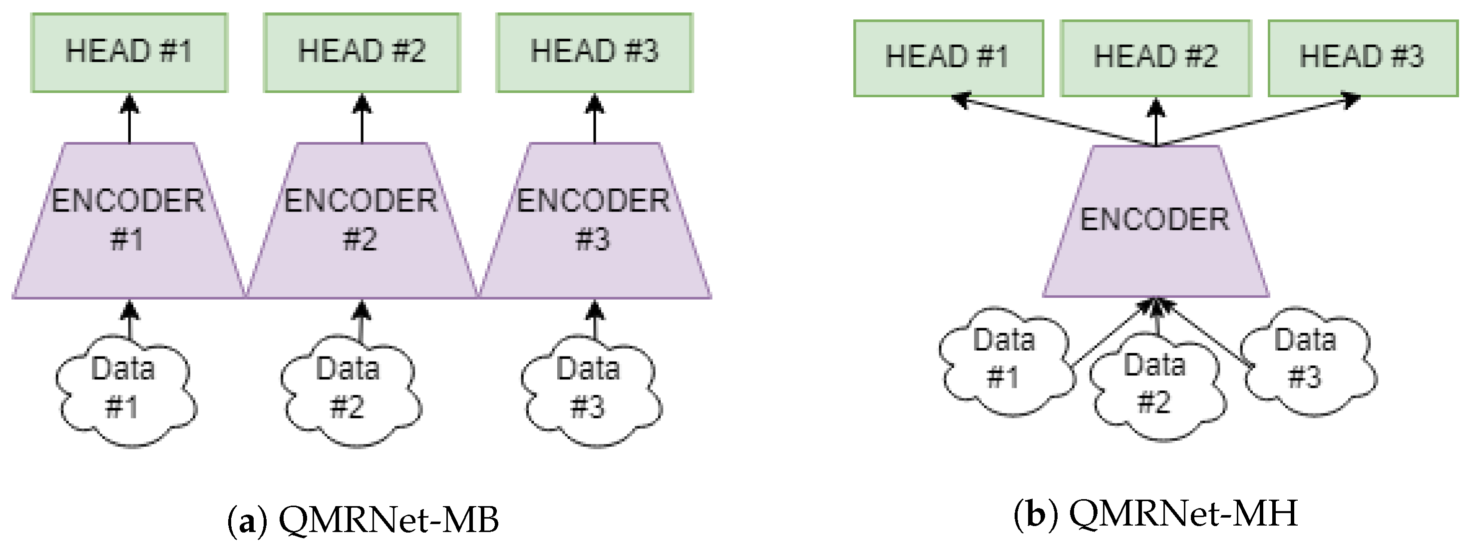
Figure 1. Architecture of QMRNet. Single-parameter QMRNet for using modified/annotated data from a unique parameter/modifier (in this case, from blur-modified images).
Remotesensing 15 02451 g001
Figure 2. Multiparameter architectures to simultaneously predict several distortions in one run. (a) Multibranch QMRNet (QMRNet-MB), example with 3 stacked QMRNets (3 encoders with 1 head each). (b) Multihead QMRNet (QMRNet-MH), example with 3 heads.
Remotesensing 15 02451 g002
Figure 3. Super-resolution model pipeline (encoder–decoder for autoencoders and generator–discriminator for GANs) with ad hoc QMRNet loss optimization. Note that all losses (i.e., L D A d v , L G P e r c and L G Q M R ) are considered for the case of MSRN optimization with QMRNet; see Section 4.4.
Remotesensing 15 02451 g003
Figure 4. Correct and incorrect prediction examples of QMRNet on Inria-AILD-180 validation (crop resolution, i.e., R = 128 × 128) given interval rank error (classification label distance between GT and prediction, maximum is N for each net, i.e., 50 for blur, 10 for sharpness and 40 for snr and rer). medR is the overall median rank (err).
Remotesensing 15 02451 g004
Figure 5. Examples of super-resolving original UCMerced images (with a crop zoom, i.e., 128 × 128) and each SR algorithm output. Inputs (Original  I H R ) without downsampling (i.e., super-resolving x3). In rows 6–10 are colormaps of the sum of differences ( Δ R + Δ G + Δ B) with respect to Original  I H R .
Remotesensing 15 02451 g005
Figure 6. Examples of super-resolving original XView images (with a crop zoom, i.e., 128 × 128) and each SR algorithm output. Inputs (Original  I H R ) without downsampling (i.e., super-resolving x4). In rows 6–10 are colormaps of the sum of differences ( Δ R + Δ G + Δ B) with respect to Original  I H R .
Remotesensing 15 02451 g006
Figure 7. Low-resolution examples of Inria-AILD-180-val images (crops of 256 × 256) and each SR algorithm output. LR (corresponding to input on algorithms I L R ) is the downsampling x3 of I H R . In rows 6–10 are colormaps of the sum of differences ( Δ R + Δ G + Δ B) with respect to Original  I H R .
Remotesensing 15 02451 g007
Figure 8. Scatter plots of metric comparison on super-resolving (x4) UCMerced dataset.
Remotesensing 15 02451 g008
Figure 9. Validation of QMRLoss optimizing MSRN in super-resolution of Inria-AILD-180. Note that the training/validation regime was conducted over Inria-AILD-180 with 100-20 image splits and crops set to 64 × 64, 128 × 128, 256 × 256 and 512 × 512.
Remotesensing 15 02451 g009
Figure 10. Examples of Inria-AILD-180-test images (with a crop zoom of 256 × 256) and each QMRNet algorithm output (QMRLoss L 1 ). Inputs (Original  I H R ) without downsampling (i.e., super-resolving x3). In rows 6–10 are colormaps of the sum of differences ( Δ R + Δ G + Δ B) with respect to Original  I H R .
Remotesensing 15 02451 g010
Figure 11. Examples of UCMerced images (with a crop zoom of 96 × 96) and each QMRNet algorithm output (QMRLoss L 1 ). Inputs (Original  I H R ) without downsampling (i.e., super-resolving x4). In rows 6–10 are colormaps of the sum of differences ( Δ R + Δ G + Δ B) with respect to Original  I H R .
Remotesensing 15 02451 g011
Figure 12. Examples of UCMerced images (with a crop zoom of 96 × 96) and each QMRNet algorithm output (QMRLoss L 1 ). Inputs (Original  I H R ) without downsampling (i.e., super-resolving x4). In rows 6–10 are colormaps of the sum of differences ( Δ R + Δ G + Δ B) with respect to Original  I H R .
Remotesensing 15 02451 g012
Table 1. List of datasets used in our experimentation. We show 12 subsets collected from 8 datasets provided by 5 satellites and EO stations.
Dataset-Subset#Set/#TotalGSDResolutionSpatial CoverageYearProvider
USGS279/27930 cm/px5000 × 5000349 km 2 (US regions)2000USGS (LandSat)
UCMerced-380380/210030 cm/px256 × 2561022/5652 (US regions)2010USGS (LandSat)
UCMerced-21002100/210030 cm/px232 × 2325652 km 2 (US regions)2010USGS (LandSat)
Inria-AILD-180-train100/36030 cm/px5000 × 5000405/810 km 2 (US and Austria)2017arcGIS
Inria-AILD-180-val20/36030 cm/px5000 × 5000405/810 km 2 (US and Austria)2017arcGIS
Inria-AILD-180-test180/36030 cm/px5000 × 5000405/810 km 2 (US and Austria)2017arcGIS
ECODSE-hs (C = 426)43/129∼60 cm/px80 × 8037/37 km 2 (Florida, US)2018OSBS
Shipsnet-Scenes7/73 m/px3000 × 150028 km 2 (San Francisco Bay)2018Open California
Shipsnet-Ships4000/40003 m/px80 × 8028 km 2 (San Francisco Bay)2018(Planetscope)
DeepGlobe469/114631 cm/px2448 × 2448703/1.717 km 2 (Germany)2018Worldview-3
Xview-train846/112730 cm/px5000 × 50001050/1.400 km 2 (Global)2018WorldView-3
Xview-validation281/112730 cm/px5000 × 5000349/1.400 km 2 (Global)2017WorldView-3
Table 2. List of modifier parameters used in QMRNet. These modify the input images and annotate them to provide training and test data for the QMRNet. Distinct intervals have been selected according to the precision and variability of the modification. represents closest values to G T .
AlgorithmAcronymParameters#Intervals (N)RangeProperties
Gaussian Blur b l u r Blur Sigma ( σ )500.0 to 2.5 Q u a l i t y , D i s t o r t i o n
Gaussian SharpnessFSharpness Factor (F)91.0 to 10.0 Q u a l i t y , D i s t o r t i o n
Ground Sampling DistanceGSDGSD or scaling100.30 to 0.60
(×1…×2)
Q u a l i t y , D i s t o r t i o n
Relative Edge Response r e r RER (MTF-Sharpness)400.15 to 0.55 Q u a l i t y , D i s t o r t i o n
Signal-to-Noise Ratio s n r Noise (Gaussian) Ratio4015 to 30 Q u a l i t y , D i s t o r t i o n
Table 3. Examples of Inria-AILD crops from modified images for each modifier (see Table 2).
Original LowerDistortion Higher
Blur ( σ )Remotesensing 15 02451 i001
σ = 1.0
Remotesensing 15 02451 i002
σ = 1.5
Remotesensing 15 02451 i003
σ = 2.0
Remotesensing 15 02451 i004
σ = 2.5
Sharpness (F)Remotesensing 15 02451 i005
F = 1.0
Remotesensing 15 02451 i006
F = 2.0
Remotesensing 15 02451 i007
F = 5.0
Remotesensing 15 02451 i008
F = 10.0
GSDRemotesensing 15 02451 i009
30
zoom (×800)
Remotesensing 15 02451 i010
36 . 6
zoom (×720)
Remotesensing 15 02451 i011
50
zoom (×506)
Remotesensing 15 02451 i012
60
zoom (×400)
RERRemotesensing 15 02451 i013
0.55
Remotesensing 15 02451 i014
0.30
Remotesensing 15 02451 i015
0.25
Remotesensing 15 02451 i016
0.15
SNRRemotesensing 15 02451 i017
30
Remotesensing 15 02451 i018
25
Remotesensing 15 02451 i019
20
Remotesensing 15 02451 i020
15
Table 4. Validation metrics for QMRNet (ResNet18) with all modifiers in Inria-AILD-180-test. Note that R (height × width) defines the resolution input of the network, in each case 1024 × 1024, 512 × 512, 256 × 256, 128 × 128 and 64 × 64. Underline represents top-1 best performance. Italics represents same value for most cases.
ParameterR (H × W)medRR@1R@5R@10F-ScoreAUC
blur64 × 642.17038.37%88.51%97.96%16.55%59.03%
(N = 50)128 × 1281.02164.42%98.44%99.85%25.82%62.20%
256 × 2560.93673.05%99.35%99.91%33.40%66.04%
512 × 5120.98970.27%99.32%100.0%36.11%72.18%
1024 × 10240.78883.04%99.65%100.0%42.56%72.83%
F64 × 641.13160.01%99.25%100.0%31.30%62.22%
(N = 9)128 × 1281.00264.78%99.92%100.0%33.73%63.60%
256 × 2561.02163.66%99.54%100.0%35.22%64.62%
512 × 5120.84972.59%99.76%100.0%40.56%68.65%
1024 × 10240.64380.28%99.85%100.0%50.96%75.45%
GSD64 × 640.000100.0%100.0%100.0%100.0%100.0%
(N = 10)128 × 1280.000100.0%100.0%100.0%100.0%100.0%
256 × 2560.000100.0%100.0%100.0%100.0%100.0%
512 × 5120.000100.0%100.0%100.0%100.0%100.0%
1024 × 10240.000100.0%100.0%100.0%100.0%100.0%
snr64 × 641.37451.44%84.92%97.97%25.57%63.06%
(N = 40)128 × 1281.39652.97%87.82%98.35%27.66%64.75%
256 × 2561.11362.65%90.12%97.25%35.60%68.93%
512 × 5121.07368.30%99.43%100.0%33.29%67.50%
1024 × 10240.92475.69%99.95%100.0%35.93%70.52%
rer64 × 641.51249.90%89.33%98.84%22.95%62.06%
(N = 40)128 × 1285.31918.79%53.78%77.79%6.95%52.28%
256 × 2561.32852.91%93.92%99.64%24.97%63.68%
512 × 5121.26857.71%94.83%99.76%28.71%68.06%
1024 × 10241.13063.06%96.53%99.98%28.88%65.00%
Table 5. Validation metrics for multiparameter prediction with QMRNet-MH (multihead) and QMRNet-MB (multibranch) in Inria-AILD-180-test. Note: QMRNet-MB (one QMRNet branch per parameter) validation is equivalent to running several parameters from Figure 4 jointly. Underline represents top-1 best performance. Italics represents same value for most cases.
ParameterR (H × W)medRR@1R@5R@10F-ScoreAUC
QMRNet-MHblur + rer128 × 1281.84945.56%89.64%98.72%20.35%60.97%
(N = 50 + 40)256 × 2561.42753.63%95.69%99.71%25.49%64.61%
512 × 5121.36557.70%93.52%95.65%28.80%65.33%
F + GSD128 × 1280.05598.39%100.0%100.0%88.61%95.47%
(N = 9 + 10)256 × 2560.52182.75%99.93%100.0%66.17%81.32%
512 × 5120.67478.93%99.42%100.0%64.28%80.23%
snr + rer128 × 1281.99844.24%86.56%97.60%20.90%61.10%
(N = 40 + 40)256 × 2562.10944.37%85.33%96.96%20.88%60.87%
512 × 5121.58852.55%92.18%98.85%26.67%65.17%
QMRNet-MBblur + rer128 × 1283.17041.61%76.11%88.82%16.39%57.24%
(N = 50 + 40)256 × 2561.13262.98%96.64%99.78%29.19%64.86%
512 × 5121.12863.99%97.08%99.88%32.41%70.12%
F + GSD128 × 1280.50182.39%99.96%100.0%66.87%81.8%
(N = 9 + 10)256 × 2560.51081.83%99.77%100.0%67.61%82.31%
512 × 5120.42486.30%99.88%100.0%70.28%84.33%
snr + rer128 × 1283.35735.88%70.80%88.07%17.31%58.52%
(N = 40 + 40)256 × 2561.22057.78%92.02%98.45%30.29%66.30%
512 × 5121.17063.01%97.13%99.88%31.0%67.78%
Table 6. Validation metrics in ECODSE Competition hyperspectral image dataset with crops of 80 × 80 and 426 bands ranging from 383 to 2.512 nm with a spectral resolution of five nm.
ParameterR (H × W)medRR@1R@5R@10F-ScoreAUC
hs (C = 426)rer (N = 40)80 × 805.4516.75%51.69%73.94%6.41%52.00%
snr (N = 40)80 × 804.7018.75%57.81%89.45%6.48%52.04%
Table 7. Mean IQA results of datasets given QMRNet(ResNet18) trained over 180 images (Inria-AILD-180-train) and 5 modifiers. Underline represents top-1 best performance. Italics represents same value for most cases.
Datasetblur↓snr rer F GSD↓Score↑
USGS1.01926.1110.4671.0000.3000.896
UCMerced-3801.00028.1210.4701.5630.3000.878
UCMerced-21001.00024.9940.4591.1940.3000.896
Inria-AILD-180-test1.02130.00.4881.0000.3000.887
Inria-AILD-180-train1.00030.00.5151.0000.3000.904
Shipsnet-Ships1.00027.5160.4831.2810.3000.881
shipsnet-Scenes1.00030.000.4993.2500.3000.846
DeepGlobe1.00030.00.5051.2810.3000.892
XView-train1.00030.00.5071.0000.3000.899
XView-validation1.00030.00.5031.0000.3000.898
Table 8. Mean no-reference Quality Metric Regression (QMRNet trained on Inria-AILD-180-train) metrics on super-resolution of downsampled inputs in UCMerced-380. Bold represents having lower distortion than HR. Underline represents top-1 best performance. Italics represents the same value for most cases.
Algorithmblur↓snr rer F GSD↓Score↑
HR1.00028.1210.4701.5630.3000.878
x2LR x 2 1.10328.9970.3661.0000.3000.820
FSRCNN1.00030.00.4902.6990.3000.853
SRGAN1.00030.00.4111.1600.3000.848
M S R N 1 1.14129.120.3441.0000.3000.804
M S R N 2 1.03628.690.4311.0180.3000.863
M S R N 3 1.10930.00.3411.0000.3000.802
ESRGAN1.08428.8740.3581.0000.3000.820
CAR1.00026.0610.4992.7760.3000.876
LIIF1.08929.5580.3481.0000.3000.810
x3LR x 3 1.14929.9370.2741.0000.3000.763
FSRCNN1.11429.9370.3231.0000.3000.793
SRGAN1.07430.00.3471.0000.3000.809
M S R N 1 1.14230.00.2771.0000.3000.765
M S R N 2 1.02530.00.3101.0000.3000.798
M S R N 3 1.03430.00.3101.0000.3000.796
ESRGAN1.33229.5610.3091.0300.3000.758
CAR1.00028.1450.4201.0710.3000.864
LIIF1.08929.5580.3481.0000.3000.810
x4LR x 4 1.62030.00.2021.0000.3000.664
FSRCNN1.56329.9370.2871.0000.3000.715
SRGAN1.36830.00.2901.0000.3000.741
M S R N 1 1.58230.00.2061.0000.3000.672
M S R N 2 1.50530.00.1851.0000.3000.671
M S R N 3 1.48430.00.2311.0000.3000.697
ESRGAN1.33229.5610.3091.0300.3000.758
CAR1.03930.00.3711.0000.3000.826
LIIF1.46729.4950.2931.0000.3000.733
Algorithmblursnr rer F GSDScore
HR1.00028.1210.4701.5630.3000.878
x2 + blurLR x 2 + b l u r 1.44429.6840.2851.0000.3000.731
FSRCNN1.00230.00.4791.5240.3000.873
SRGAN1.07630.00.3381.0000.3000.805
M S R N 1 1.47329.750.2741.0000.3000.721
M S R N 2 1.43429.620.2861.0000.3000.733
M S R N 3 1.43430.00.2791.0000.3000.728
ESRGAN1.20830.00.2821.0000.3000.759
CAR1.01328.7500.3821.0710.3000.840
LIIF1.56830.00.2371.0000.3000.689
x3 + blurLR x 3 + b l u r 2.42030.00.1981.0000.3000.556
FSRCNN1.64930.00.2291.0000.3000.674
SRGAN1.27330.00.2431.0000.3000.731
M S R N 1 2.33930.00.1981.0000.3000.566
M S R N 2 2.32430.00.1781.0000.3000.559
M S R N 3 2.24430.00.2101.0000.3000.586
ESRGAN1.55930.00.2421.0000.3000.692
CAR1.11629.9370.3121.0000.3000.787
LIIF1.72530.00.2281.0000.3000.663
x4 + blurLR x 4 + b l u r 1.84030.00.1591.0000.3000.613
FSRCNN1.64930.00.2291.0000.3000.674
SRGAN1.62530.00.1751.0000.3000.650
M S R N 1 1.69630.00.1611.0000.3000.633
M S R N 2 1.60630.00.1551.0000.3000.642
M S R N 3 1.63030.00.1681.0000.3000.645
ESRGAN1.55930.00.2421.0000.3000.692
CAR1.32930.00.2581.0000.3000.731
LIIF1.72530.00.2281.0000.3000.663
Table 9. Mean full-reference metrics on super-resolution of downsampled inputs in UCMerced-380. Underline represents top-1 best performance.
Algorithmssim↑psnr↑swd↓fid↓mssim↑haarpsi↑gmsd↓mdsi↑
HR1.0080.000--1.001.00--
x2LR x 2 0.90130.62811250.2110.9900.9540.0140.330
FSRCNN0.43816.68223164.470.7180.5520.1550.427
SRGAN0.91931.53410100.1770.9910.9250.0150.308
M S R N 1 0.90130.17811030.2220.9900.9500.0140.329
M S R N 2 0.91731.75010170.1740.9910.9510.0130.315
M S R N 3 0.89230.41711670.2170.9870.9340.0160.339
ESRGAN0.79326.69314620.3530.9590.7370.0730.370
CAR0.82726.28512820.4220.9680.8310.0640.354
LIIF0.86029.64512360.2200.9780.8920.0360.360
x3LR x 3 0.77827.00416190.3860.9560.8010.0720.401
FSRCNN0.83928.98213280.2430.9730.8650.0420.367
SRGAN0.81127.63314560.3320.9610.7960.0530.386
M S R N 1 0.70024.36818640.5020.9180.6660.1280.420
M S R N 2 0.69924.16918000.5130.9180.6630.1280.415
M S R N 3 0.70124.26118380.4880.9180.6620.1280.418
ESRGAN0.82528.38713710.2620.9700.8480.0490.366
CAR0.72123.27316780.7080.9250.7000.1110.394
LIIF0.86029.64512450.2200.9780.8920.0360.360
x4LR x 4 0.68325.03119730.5690.9250.7030.1210.440
FSRCNN0.81928.22314010.2780.9690.8430.0500.372
SRGAN0.72125.84417500.4680.9360.7160.0960.428
M S R N 1 0.60022.69121420.7430.8690.5730.1640.453
M S R N 2 0.59922.58220940.7520.8700.5700.1640.451
M S R N 3 0.60222.65121560.7260.8710.5690.1650.454
ESRGAN0.82528.38713490.2620.9700.8480.0490.366
CAR0.62421.82519530.9100.8870.6200.1500.421
LIIF0.84128.70813160.2540.9740.8660.0430.367
Algorithmssimpsnrswdfidmssim↑haarpsi↑gmsd↓mdsi↑
HR1.0080.000--1.001.00--
x2 + blurLR x 2 + b l u r 0.82227.87615040.3560.9680.8540.0510.385
FSRCNN0.37216.42524954.890.6620.5020.1840.447
SRGAN0.83628.13513980.3490.9660.8260.0520.376
M S R N 1 0.82527.57414850.3770.9680.8550.0490.383
M S R N 2 0.84628.63714090.3070.9720.8670.0450.372
M S R N 3 0.81727.85215290.3550.9650.8400.0530.389
ESRGAN0.77426.75416570.4010.9550.7380.0750.404
CAR0.90330.71611560.1970.9840.9150.0340.326
LIIF0.74826.31217690.5080.9390.7740.0880.422
x3 + blurLR x 3 + b l u r 0.69125.05420030.6140.9180.7160.1150.444
FSCNN0.74126.10718040.5130.9380.7640.0880.423
SRGAN0.70525.08919110.6370.9150.7030.1070.443
M S R N 1 0.64523.80321310.7060.8920.6390.1430.455
M S R N 2 0.64923.73120500.7140.8950.6410.1410.450
M S R N 3 0.64923.83221130.6810.8940.6390.1420.454
ESRGAN0.75226.31417700.4880.9410.7700.0850.419
CAR0.78326.90916160.3780.9550.8010.0700.405
LIIF0.74826.33717980.5000.9390.7770.0860.421
x4 + blur L R x 4 + b l u r 0.97238.5998970.0460.9920.9400.0310.248
FSRCNN0.97737.2108340.0620.9920.9500.0220.226
SRGAN0.96234.76110500.0830.9860.8670.0330.265
M S R N 1 0.90930.11512770.1120.9550.7560.0950.316
M S R N 2 0.90129.51313500.1500.9550.7500.0960.317
M S R N 3 0.90929.88812810.1200.9550.7490.0960.319
ESRGAN0.97337.2028760.0620.9920.9450.0240.236
CAR0.91630.06713710.2130.9640.8310.0740.309
LIIF0.99447.3174200.0320.9990.9930.0030.166
Table 10. Mean no-reference noise (SNR) and contour sharpness (RER, MTF, FWHM) metrics on super-resolution of downsampled inputs in UCMerced-380. Underline represents top-1 best performance.
AlgorithmSNR M d n SNR M RER X Y MTF X Y FWHM X Y
HR20.78828.814503.5124.51692
x2LR x 2 31.36143.217367.5302379.5
FSRCNN10.83011.016471.54373038.5
SRGAN28.69935.223497119.51730
M S R N 1 33.18845.94135624.52450
M S R N 2 30.11440.626376352329.5
M S R N 3 34.21743.851367.529.52374
ESRGAN23.91631.614382352269
CAR15.66026.5065531661484
LIIF44.27356.133459.5921909
x3LR x 3 45.3354.317317.5932754
FSRCNN39.7245.69222.51912132
SRGAN43.7549.17432.51872015.5
M S R N 1 43.88252.050321.515.52743.5
M S R N 2 37.70746.747340.5192571
M S R N 3 44.57952.747345.520.52532.5
ESRGAN28.5839.973401152562.5
CAR25.2039.45522.5261.51617
LIIF44.2756.13460.52521903.5
x4LR x 4 49.18357.35127963150
FSRCNN30.79741.584325.5142678
SRGAN50.25855.28236628.52385.5
M S R N 1 51.87560.0432816.53113
M S R N 2 45.08452.37329382987
M S R N 3 53.52361.69129882936
ESRGAN28.58439.97434018.52560
CAR30.19347.106485.5113.51793
LIIF35.37549.543342102546
AlgorithmSNR M d n SNR M RER X Y MTF X Y FWHM X Y
HR20.78828.814503.5124.51692
x2 + blurLR x 2 + b l u r 40.86449299132804.5
FSRCNN11.31411.529289.58.53046.5
SRGAN41.63049.499400562258
M S R N 1 43.34653.85830610.52865.5
M S R N 2 39.28752.993317.5142766
M S R N 3 44.00753.984314.512.52791
ESRGAN42.65655.710318132770.5
CAR33.73747.754446.576.51939
LIIF58.28973.03029811.52975
x3 + blurLR x 3 + b l u r 57.19365.361287.553107.5
FSRCNN52.59866.357285.583083.5
SRGAN55.65864.598354.527.52515
M S R N 1 54.60162.769290.511.53076.5
M S R N 2 50.25760.81297122997.5
M S R N 3 58.37766.545302132954.5
ESRGAN51.33066.647291103036
CAR50.69666.709398.5482209.5
LIIF56.19464.36228373119.5
x4 + blurLR x 4 + b l u r 65.08973.257268.57.53311.5
FSRCNN53.43068.24629083038.5
SGAN62.23670.854316.5142806
M S R N 1 63.81071.978279.5133579.5
M S R N 2 54.68263.786282.58.53445
M S R N 3 70.04878.216288.59.53308
ESRGAN53.55967.79329243011.5
CAR60.48383.280359.5302471
LIIF56.19464.362282.56.53120
Table 11. Test metrics on super-resolution (super-resolving original input x3 or using downsampled inputs x3) using MSRN backbone +QMRLoss in UCMerced-380. Q M R L o s s L 1 computation over Inria-AILD-180-train on distinct QMRNets (for b l u r , r e r and s n r ) using crops of R = 256 × 256. Note that here we are testing MSRN + QMRLoss over UCMerced samples while QMRNet’s training is on Inria-AILD. Bold represents having lower distortion than HR. Underline represents top-1 best performance. Italics represents the same value for most cases.
Algorithmblur↓snr rer F GSD↓Score↑ssim↑psnr↑swd↓fid↓SNR M d n RER X Y MTF X Y FWHM X Y
HR1.00028.120.4701.5630.3000.8781.0080.00-0.07920.790.5020.1251.709
Original x3MSRN v a n i l l a 1.00028.180.4641.3550.3000.8790.71723.6516340.41121.280.5010.1241.712
+QMRLoss σ , L 1 1.00026.810.5212.2850.3000.8940.60821.2217840.81513.720.5570.1811.505
+QMRLoss G S D , L 1 1.00027.620.5201.9650.3000.8960.60121.4017990.74512.810.5730.1951.447
+QMRLoss F , L 1 1.00026.620.5241.9470.3000.9040.60521.4117860.79013.370.5660.1891.473
+QMRLoss r e r , L 1 1.00026.810.5242.1780.3000.8980.60321.1017880.85013.240.5580.1801.493
+QMRLoss s n r , L 1 1.00026.750.5212.2320.3000.8950.60421.1217940.85013.700.5650.1881.471
x3LR x 3 1.14929.940.2741.0000.3000.7630.77827.0016330.38645.330.2970.0082.946
MSRN v a n i l l a 1.14230.000.2771.0000.3000.7650.70024.3718460.50243.880.3010.0102.900
+QMRLoss σ , L 1 1.03130.000.3071.0000.3000.7950.70624.3518040.47936.290.3140.0112.782
+QMRLoss G S D , L 1 1.03829.940.3471.0000.3000.8150.70124.3318140.48235.020.3300.0162.664
+QMRLoss F , L 1 1.02829.750.4121.0000.3000.8490.69624.2618030.48334.880.3280.0162.674
QMRLoss r e r , L 1 1.03630.000.3041.0000.3000.7930.70424.3718100.48236.320.3140.0112.787
+QMRLoss s n r , L 1 1.03630.000.3051.0000.3000.7930.70624.3417970.48135.080.3150.0122.773
Disclaimer/Publisher’s Note: The statements, opinions and data contained in all publications are solely those of the individual author(s) and contributor(s) and not of MDPI and/or the editor(s). MDPI and/or the editor(s) disclaim responsibility for any injury to people or property resulting from any ideas, methods, instructions or products referred to in the content.