Abstract
Shape segmentation in urban environments forms the foundation for tasks such as classification and reconstruction. Most artificial buildings with complex structures are composed of multiple simple geometric primitives. Based on this assumption, this paper proposes a divisive hierarchical clustering algorithm that uses shape classification and outliers reassignment to segment LiDAR point clouds in order to effectively identify the various shapes of structures that make up buildings. The proposed method adopts a coarse-to-fine strategy. Firstly, based on the geometric properties of different primitives in a Gaussian sphere space, coarse extraction is performed using Gaussian mapping and the DBSCAN algorithm to identify the primary structure of various shapes. Then, the error functions are constructed after parameterizing the recognized shapes. Finally, a minimum energy loss function is built by combining the error functions and binary integer programming (BIP) to redistribute the outlier points. Thereby, the accurate extraction of geometric primitives is achieved. Experimental evaluations on real point cloud datasets show that the indicators of precision, accuracy, and F1 score of our method are 0.98, 0.95, and 0.96 (point assignment) and 0.97, 0.95, and 0.95 (shape recognition), respectively. Compared with other state-of-the-art methods, the proposed method can efficiently segment planar and non-planar structures with higher quality from building point clouds.
1. Introduction
The detection of building structures is the basis of building digitization and the primary step in 3D urban reconstruction. With the development of sensors and platforms, 3D point clouds have become the primary data source for sensing cities, which are mainly derived from LiDAR [1] and multi-view stereo [2] datasets. LiDAR can quickly and directly acquire a 3D point cloud of a target surface via non-contact active measurement, avoiding the complicated solving of image correspondence in MVS. Due to its excellent characteristics, such as the low influence of weather, short data acquisition period, and high accuracy, LiDAR technology is gradually becoming the major data source for the 3D reconstruction of urban scenes [3,4], autonomous driving [5], and emergency response systems [6]. However, LiDAR point clouds are disordered and unsemantic, essentially comprising a downsampled representation of the 3D world geometry, and do not provide structural information about the target. Thus, point cloud segmentation is necessary prior to further applications.
Point cloud segmentation involves dividing point clouds into groups with similar properties based on spatial and geometric information [7]. Artificial buildings with complex structures can be regarded as a combination of multiple geometric primitives. Based on this assumption, point cloud segmentation can theoretically extract all building components. However, most research focuses on plane extraction and ignores other structures. In addition, the problem of assigning points at sharp features is a challenge for accurate segmentation. Therefore, this paper proposes a divisive hierarchical clustering algorithm in order to address these issues. According to the anisotropy characteristic of normal vectors, they can reflect the local orientation of the object surface, i.e., the normal vectors are consistent on the same surface, while they present a scattered distribution when dealing with sharp features or noise. Based on this fact, a two-stage clustering method is proposed in this paper to segment the building point clouds. Additionally, the major contributions of this paper are as follows:
- (1)
- A novel framework for building segmentation via shape classification and outliers reassignment is presented.
- (2)
- A coarse segmentation method based on a combination of Gaussian mapping and DBSCAN is developed. The plane, cone, cylinder, and sphere structures that make up the target are identified based on the morphological differences of different shape primitives presented in Gaussian spherical space.
- (3)
- A fine segmentation based on the BIP models is proposed. The complete segmentation is achieved by the constructed minimum energy function, which reassigns the outlier points to each recognized primitive.
The remainder of this paper is organized as follows. Section 2 provides a brief review of the existing literature on point cloud segmentation. Section 3 describes the details and key steps of the proposed segmentation approach. Section 4 shows the performance of the proposed approach on both synthetic and real point cloud datasets and presents a discussion of the method and the experimental results. Finally, we draw our conclusions in Section 5.
2. Related Works
Point cloud segmentation for buildings has been the focus of much research [8,9]. Numerous different strategies have been proposed for different scenarios and applications [10,11,12]. This section briefly reviews the segmentation methods, including region growing, model fitting, clustering, and hierarchical clustering.
2.1. Region Growing
The accuracy and efficiency of the region-growing algorithm are influenced by three factors: seed points, neighborhoods, and discriminant conditions. For the choice of seed point, the most popular current method is to select the point with the least curvature as the initial seed point during each iteration [13]. Since the seed point is located in the smoothest region, growing from it can reduce the total number of segmented fragments and thus improve the algorithm’s efficiency. Regarding the neighborhood, the traditional region-growing approach uses k-dimension trees (kd trees) [14] to search the range of k-neighborhoods (or r-balls). This approach does not consider the neighborhood’s geometric properties, which tends to produce under-segmentation or over-segmentation problems. Methods have been proposed to overcome this problem via adapting the neighborhood while considering the geometrical content [15] or via using voxels with good planarity as neighborhoods [16]. Regarding the discriminant conditions, the geometric properties of primitives such as Euclidean distance and normal vector are commonly used [17]. Moreover, there are some studies that aim to improve the region growth in other ways; for example, Zhu et al. [18] optimized the point cloud normal vectors, especially around the sharp features. Thus, the region-growing method can extract the planar structures of buildings completely. Dong et al. [19] proposed a hybrid region-growing method on LiDAR point clouds of buildings with points and surfaces as primitives to improve the algorithm’s efficiency.
2.2. Model Fitting
Most of the existing model-fitting methods rely on Hough transform (HT) [20] and random sample consensus (RANSAC) [21] algorithms. HT is a classical feature detection technique and performs well when processing 2D images. However, in 3D point clouds, the parameters of HF increase, and the algorithm’s complexity increases exponentially. Therefore, some methods enhance the performance of HT by reducing the cost of the voting process to improve efficiency, such as Randomized HT [22], Probabilistic HT (PHT) [23], and improved methods based on PHT, such as Adaptive PHT [24] and Progressive PHT [25]. These methods are applied to point cloud segmentation to identify planes [26] and geometric structures such as cylinders and cones [27]. Compared with HT, the RANSAC method greatly improves computational efficiency and is robust to noise. However, the RANSAC method is prone to generate artifacts because it strives to find a geometry with the highest number of points in each iteration. To solve this problem, Chen et al. [28] proposed an improved RANSAC algorithm with localized sampling to segment building roofs. Xu et al. [29] proposed a weighted RANSAC algorithm that considers the point-plane distance and the normal vector consistency for building plane segmentation from LiDAR point clouds. RANSAC methods have been widely applied to building roof detection [30] from LiDAR point clouds and building facade detection [31] from oblique photogrammetric point clouds.
2.3. Clustering
Euclidean distance clustering [32] is a typical clustering method that uses the Euclidean distance between points as a clustering criterion. In addition to distance, standard point cloud features include normal vector, curvature, and color. For example, Filin [33] used the curvature and color of point clouds for surface clustering. Nurunnabi et al. [34] used the curvature and normal vector to cluster the outlier points in a point cloud. Typical clustering algorithms include k-mean [35], its improvement algorithms, and mean shift [36]. K-mean requires a pre-determined number of clusters, k, and the random initialization of the cluster centers may lead to algorithm instability. To solve this issue, the ISODATA algorithm [37] adjusted the number of clustering centers by splitting and merging operations. The k-means++ algorithm [38] introduced the principle that the initial clustering centers should be as far away from each other as possible to distribute the clustering centers. In addition, density-based clustering algorithms [39,40,41] are also a popular strategy. Chen [42] used the exponential function density clustering model to extract indoor objects from LiDAR point clouds. Wang [43] improved the DBSCAN algorithm by automating the calculation of parameters to complete the segmentation of urban environments. Chen [44] introduced coplanar constraints to the DBSCAN algorithm to achieve the segmentation of building shapes. However, over-segmentation is prone to be caused when using this method alone, so it is commonly used for coarse segmentation [45] or combined with other methods [46]. Due to a scene’s complexity, it is difficult for a single clustering method to extract accurate and complete surface structures. Thus, hierarchical clustering with a combination of multiple clustering algorithms is the more popular method nowadays.
2.4. Hierarchical Clustering
The hierarchical clustering method performs the hierarchical decomposition or consolidation of data objects [47]. According to different choices, the hierarchical clustering method can be further divided into agglomerative branches [48] and divisive branches [49]. Agglomerative hierarchical clustering, which uses a bottom-up strategy, first classifies each object as a group and then merges these groups into larger groups. In contrast, divisive hierarchical clustering, which uses a top-down strategy, first classifies all objects in a group and then gradually subdivides them into smaller groups. Divisive clustering is generally more complex than agglomerative clustering because it partitions the data until each cluster contains one data item [50]. However, divisive clustering is more accurate because it considers the data’s global distribution when partitioning it into a top-level partition. Feng et al. [51] proposed a plane extraction method based on agglomerative hierarchical clustering for organized point clouds. Li et al. [52] extracted the initial planar patches via an octree-based method and then applied agglomerative hierarchical clustering to merge the adjacent planar patches for roof segmentation from airborne LiDAR. Lu et al. [53] combined pairwise linkage and divisive hierarchical clustering to extract planar structures of buildings in LiDAR point clouds. Kung et al. [54] applied agglomerative hierarchical clustering to merge the supervoxels into surfaces for iterative curve shape extraction. Hierarchical clustering can also be applied to classification and recognition. Jurado et al. [49] proposed the unsupervised classification of natural materials in a point cloud based on divisive hierarchical clustering. Zhang et al. [55] proposed an agglomerative–divisive hierarchical clustering for organ classification and fruit recognition for a whole fruit tree in a natural environment.
3. Methods
3.1. Overview of the Proposed Approach
Starting from the LiDAR point cloud, the overall workflow of our method is shown in Figure 1. The proposed method adopts a coarse-to-fine strategy and consists of two stages. In the coarse segmentation stage, because the normal vectors of the same geometric shapes are distributed centrally on the Gaussian sphere, the normal vectors of the point cloud are mapped onto the Gaussian sphere. Then, according to the different density distributions presented by the groups on the Gaussian sphere, we use the DBSCAN clustering method to classify the different shapes and complete the coarse extraction. In the fine segmentation stage, the main task consists of two components: one is to refine each shape class by combining Euclidean distance classification and parameterization; the other is to construct an optimization function, which reassigns the outliers using BIP to complete the fine segmentation.
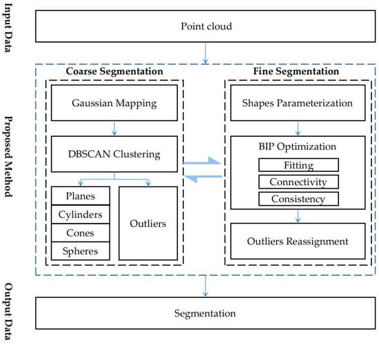
Figure 1.
Workflow of the proposed method.
3.2. Coarse Segmentation
Based on the assumption that complex buildings are composed of simple shapes, four geometric shapes are used as primitives: plane, cylindrical, conic, and spherical surfaces. A single shape can be easily identified based on the density distribution of the Gaussian sphere, as shown in Figure 2. For example, points on a plane are presented as a spot on the Gaussian sphere (Figure 2b, red point), and points on a cylindrical surface are presented as a circle at the center of the Gaussian sphere (Figure 2b, yellow ring), points on the conical surface are also presented as a circle, but its center is not at the center of the Gaussian sphere (Figure 2b, green ring), and points on the spherical surface have the same presentation on the Gaussian sphere (Figure 2b, blue sphere). However, in complex scenes, multi-directional, multi-species, and multi-scale primitives are overlapped on the Gaussian sphere, so the primary task of this method is to classify all geometric shapes.
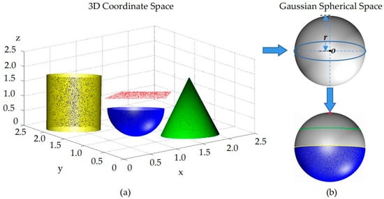
Figure 2.
The Gaussian mapping of four shapes. (a) Represents the four geometric shapes in 3D coordinate space. (b) Represents the Gaussian spherical space and the results of the four shapes after Gaussian mapping. Different colors indicate different shapes.
The Gaussian sphere is a space with a center of (0,0,0) and a radius of 1 unit. Firstly, the normal vectors of the point cloud are estimated by a PCA algorithm. The normal vector of each point conforms to nx2 + ny2 + nz2 = 1. The normal vectors of all points are mapped into the Gaussian sphere space to obtain the new point set gpi = {(nx, ny, nz); nx2 + ny2 + nz2 = 1}. Since the normal vectors of the one plane in 3D space are consistent, the density of points on the Gaussian sphere increases with the number of points on the same structure. In addition, points on structures with the same orientation but different scales will also gather on the Gaussian sphere. Thus, based on this feature, the DBSCAN method [56] is used to extract the set of points with a high-density distribution. The DBSCAN method is a density-based clustering algorithm with noise immunity that does not require one to specify the number of class species. It exploits the high-density connectivity of clusters to find high-density regions and can extract sets of arbitrary shapes. In this paper, a point-by-point traversal strategy is used, i.e., if a point is not the core point, it is ignored, and if it is, a new cluster is created, and all neighboring points are added to the cluster. If there are other core points in the neighborhood, their neighborhood points are also added to the cluster recursively. This process is repeated until there are no more points to add to the cluster. During the clustering process, the number of neighborhood points (NN) of the core points needs to be recorded. As for the neighborhood search strategy, instead of the suggested R*-tree in the original DBSCAN, the kd-tree is used for a faster k-nearest neighbor search.
To distinguish shapes, a 3D spatial point feature is introduced, which can be calculated by three eigenvalues λ1, λ2, λ3 (λ1 > λ2 > λ3) of a singular value decomposition (SVD) of the covariance matrix. When λ1 >> 0, λ2 >> 0, λ3 >> 0, the point cluster exhibits a random distribution; when λ1 >> 0, λ2 >> 0, λ3 ≅ 0, the point cluster exhibits a planar distribution; when λ1 >> 0, λ2 ≅ 0, λ3 ≅ 0, the point cluster exhibits a linear distribution; when λ1 ≅ 0, λ2 ≅ 0, λ3 ≅ 0, the point cluster exhibits a sparse spot distribution. Thus, based on these features, the measures are derived to describe the geometric properties as follows:
where Pλ indicates the probability that the geometry is similar to a plane, and a larger value of Pλ indicates a flatter local geometry; Lλ indicates the probability that the geometry is similar to a line, and a larger value of Lλ indicates a thinner local geometry. Considering the influence of noise, two empirical thresholds are set. λ > 0.8 means λ >> 0, and λ < 0.2 means λ ≅ 0.
Finally, shape classification is achieved via a step-by-step analysis of the structure. The specific procedure is as follows:
- (1)
- The DBSCAN algorithm is executed in the Gaussian sphere space to obtain multiple clusters ς = {G1, G2, …, Gi};
- (2)
- For a cluster Gi, a spatial resampling is performed with an interval of 0.01 m, and then a point in Gi is selected and searched for points within the radius of r/2;
- (3)
- After calculating the eigenvalues of the searched points, if all three eigenvalues are less than 1, Gi is a spot, and the corresponding point groups in the 3D point cloud space are marked as planes. Then, the shape features are derived using Equation (1); if Pλ < Lλ, Lλ is linear, its radius is calculated. If the radius is 1 m, the corresponding points groups in the 3D point cloud space are marked as cylinders. If the radius is less than 1 m, those groups are marked as cones. Note that when Gi is judged to be linear, this cluster may contain another spot cluster, as shown in Figure 3. The generated local highlight phenomenon is evident in the circle of Figure 3c, so we count the average value of NN for the core points in Gi. If the NN of the core point is larger than the average value, it and its neighbors are marked as local highlighting regions and selected as a new cluster;
- (4)
- The 3D spherical surface is also presented as a uniformly distributed spherical structure in the Gaussian sphere space. Thus, for the points of the spherical surface, the NN of core points should be close. In the Gaussian sphere space, after excluding the identified points, the remaining points connected and have close NN values to each other are selected as clusters and marked as spherical shapes.
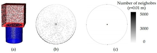
Figure 3.
The clustering results of cylinder and cube point clouds in Gaussian sphere space. (a) Represents the point clouds of cylinders and cubes with 40,000 points. (b) Represents the mapping of the point clouds in a Gaussian sphere. (c) Represents the clustering results, and the colors are rendered using the point density.
3.3. Fine Segmentation
3.3.1. Shape Parameterization
After completing the above processes, the point cloud can be divided into classified shapes SPs and outlier points Φ. SPi = {sp1, sp2,…,spj}, all the spj belong to the same type of primitive with different parameters. To facilitate the subsequent parameterization, each shape needs to be extracted separately. Firstly, a point p is selected from SPi, and the distance from its neighboring points to p is calculated. If the distance is less than the threshold value of 2 × RES, the neighboring point is divided into spj, where Res denotes the average point distance of the point cloud. Then, the points other than p in spj are selected, and the above process is repeated until the number of elements in spj does not increase. This procedure is repeated until all clusters are completed. The remaining points are stored in the Φ. Further parameter calculation of spj is needed for each type.
Planes
Three non-collinear points can theoretically calculate the plane parameters ax + by + cz + d = 0. Considering the effect of noise, the least squares solver is used to calculate the parameters to ensure that the solved plane can optimally fit the point cloud, so the objective function is:
where , , are the centers of points. This is a typical min||Ax|| problem. The SVD decomposition is performed on matrix A. The eigenvector corresponding to the smallest eigenvalue is (a, b, c), and then d is calculated using the center of points.
Cylinder
Solving cylinder parameters consists of two parts: the determination of the initial parameter values and the establishment of the error equation. According to the geometric characteristics of the cylindrical surface, the distance from the point (x, y, z) on the cylindrical surface to the axis vectors u is cylindrical radii r. Then, according to this characteristic, the error equation is established as follows:
After linearization, the solution can also be solved using the least squares method. The initial values of the axes u0 can be derived from the normal vector of the corresponding cluster Gi on the Gaussian sphere. Then, a planar circle can be obtained by slicing the points spj from the direction perpendicular to the axis u0. The radius and center of the ring are the initial r0 and the point m0 on the axis u0.
Cone and Sphere
The parameters of the cone include the vertex v, cone angle θ, and axis vector u, and the parameters of the sphere include the center coordinates o and radius r. Considering the existence of cone frustum, the coordinates of cone vertices are difficult to initialize, which leads to the low efficiency of the least squares solution. Similarly, there are mostly incomplete spherical structures, and it is challenging to initialize the spherical center. Therefore, for the parameterization of these two primitives, this paper uses a RANSAC-based method [57] to iteratively select several points randomly in the cluster for parameter solution and then selects the optimally fitted model as the final result.
3.3.2. Outlier Reassignment
For further accurate segmentation, outlier points need to be reassigned. A popular method uses the distance from the point to the model as the criterion. However, there are some disadvantages when relying on this single metric, such as the selection of a threshold value and spurious surfaces caused by local fitting. Thus, three metrics are designed to reassign the outlier points as follows.
Fitting
The point p(x, y, z) fitted into the shape model should ensure the minimum distance to this shape. For different primitives, the distances from point p to the model are calculated differently. We mark Dp, Dcy, Dco, and Ds to denote the distances of point-to-plane, point-to-cylinder, point-to-cone, and point-to-sphere, as shown in Equation (4):
where m is the point on the axis of the cylinder, u1 and u2 are the axes of the cylinder and cone, respectively, v is the vertex of the cone, o is the center of the sphere, and r1 and r2 are the radii of the cylinder and sphere, respectively. Thus, the construction of the metric is Equation (5), where Dt∈{Dp, Dcy, Dco, Ds}.
Connectivity
To avoid spurious facets, the points of the same shape must be connected to each other. For points pi, pj, and pk, the neighbors of their 2 × RES range are used as buffers I, J, and K. If I∩J1∅, and J∩K1∅, I and K are connected. Then, a connected set Π is built. If Π contains the points of the shape, then Π is connected with the shape. The metric is Equation (6):
Consistency
If a point has the minimum distance to two shapes simultaneously, then this point can be judged as the junction of these shapes. Voiding edge jaggedness, the points on the intersection should be classified as the same shape. The metric is Equation (7), where ξi and ξj denote the shape to which the point belongs:
Finally, a minimum energy function based on the BIP model is used to discriminate the outlier points. BIP is a special linear optimization with variables xi∈{0, 1}. A multidimensional variable ξ = {l1, l2, …, ln}, li∈{0, 1} is constructed whose dimension is the number of detected shapes. Different values of ξ represent different shapes; for example, ξ1 = {1, 0, 0, …, 0} and ξ2 = {0, 1, 0, …, 0} denote two shapes. Since a point in Φ can be assigned to only one shape, it is necessary to constrain |ξ| = 1. Finally, the minimum energy function is constructed as follows:
4. Experiments and Discussion
To verify the efficiency and robustness of the proposed method, experiments are conducted on both synthetic data and real-point cloud datasets. The proposed approach was implemented with C++ in Windows and carried out on a computer with an Intel Core i9-9900K processor and 64 GB of RAM. In addition, qualitative comparisons are performed between the proposed method and four popular and recent approaches: region-growing (RG), RANSCA, PLINKAGE [53], and QTPS [58]. The region-growing and RANSAC methods are the most popular, widely adopted algorithms for point cloud segmentation. PLINKAGE and QTPS are recently published hierarchical clustering algorithms. All point cloud datasets are preprocessed for normal vector estimation using the PCA algorithm.
4.1. Evaluation Metrics
To evaluate the segmentation quality, four traditional metrics are employed, i.e., Precision, Recall, and F1-Score.
We calculated the corresponding metrics for points and surfaces, respectively. For the metric of points (Precisionp, Recallp, F1p), TP (true positive) indicates the number of points correctly assigned; FN (false negative) indicates the number of points present in the ground-truth data but not assigned; and FP (false positive) indicates the number of points incorrectly assigned. For the metrics of shapes (Precisions, Recalls, F1s), TP is the number of shapes correctly detected; FN is the number of shapes in the ground-truth model but not detected; FP is the number of shapes falsely detected.
4.2. Experiments on Synthetic Data
Six synthetic datasets are used to test the proposed method. These datasets are generated from modeling in Sketchup and sampling points in CloudCompare. The detailed data descriptions are listed in Table 1.

Table 1.
Details of synthetic datasets.
The experimental results are shown in Figure 4. The planar structures appear clustered as points on the Gaussian sphere, while the points at the edges are presented as isolated points on the Gaussian sphere due to the scattering of their normal vectors, as shown in Figure 4b. Then, after the clustering process, various geometric primitives are identified, while the outlier points are mainly distributed at the edges of the shapes, as shown in Figure 4c. These phenomena are exactly as expected. Finally, the outlier points are reassigned to achieve the fine segmentation of each shape, as shown in Figure 4d. Since there is no noise in the synthetic data, the proposed method can segment all points correctly. In addition, the execution time of the algorithm is shown in Figure 5. The algorithm’s time consumption is positively related to the number of point clouds.
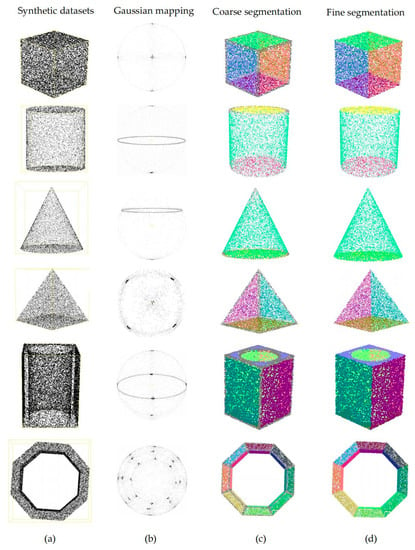
Figure 4.
Shapes segmentation on synthetic datasets. (a) Point cloud. (b) Gaussian mapping. (c) Coarse segmentation, in which gray points denote outlier points. (d) Fine segmentation.
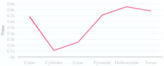
Figure 5.
The execution time (in seconds) of different data.
The shape detection ability of the comparison methods is shown in Figure 6. The RG method can segment different shapes, including plane and curved surfaces but cannot handle boundaries. The RANSAC method can segment single shapes but performs weakly when handling mixed shapes and is prone to over-segmentation. The PLINKAGE method produces under-segmentation when dealing with mixed shapes. The QTPS method has strong planar segmentation ability and offers the strongest boundary handling capability compared to the other three methods, but it cannot segment curved surfaces.
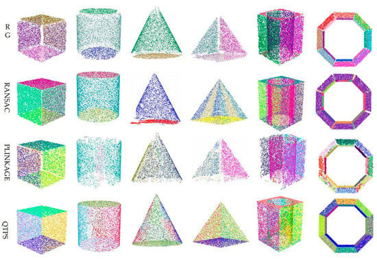
Figure 6.
Shape segmentation of comparison methods.
The robustness to noise is essential for the point cloud segmentation method. Random noise is inevitable in the real point cloud and is difficult to evaluate quantitatively. To evaluate the robustness of the proposed algorithm, the Torus point cloud is selected as the experimental object, and we add different noise levels following a Gaussian distribution. The percentages of the noise are 10%, 20%, 30%, 40%, and 50%, and the standard deviations (s.d.) of the noise are 3 mm, 6mm, and 10 mm.
The execution time of the proposed algorithm at different noise levels is shown in Figure 7, which clearly shows that the time consumption is proportional to the number of noise points and the standard deviation of the noise. There are two reasons for this result: (1) the more noise points there are, the more data processing is necessary, which increases the processing time; (2) the larger the standard deviation of the noise, the larger the bias of the normal vectors calculated by PCA. The PCA is a least-squares procedure fitting to the local surface with robustness. Still, when the standard deviation of the noise is too large, the accuracy of the estimated normal vectors decreases. Thus, the larger the standard deviation of the noise, the larger the bias of the estimated normal vectors, which in turn leads to more isolated points on the Gaussian sphere and more time being required to reassign these isolated points.
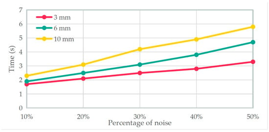
Figure 7.
The execution time (in seconds) of the algorithm at different noise levels.
The accuracy metrics of the segmentation results at different noise levels are shown in Figure 8. The figure shows that the proposed algorithm gives excellent segmentation results when the percentage of additional noise is less than 50%, and the noise standard deviation is less than 10 mm. In these cases, the noise not located on the plane boundary is fitted into the plane model and does not influence the model parameters. The noise located on the plane boundary may be reassigned incorrectly, so it causes some fluctuation in the precision at different noise levels. However, when the percentage of additional noise is 50%, and the standard deviation is 10 mm, the precision decreases substantially. By analyzing the procedures and the final segmentation results, there is over-segmentation in the result, which is caused by the confusion of the inner and outlier points on the Gaussian square. In addition, our method uses the minimum energy function to reassign the outlier points, so the experimental result for Recall is 1 because FN = 0.
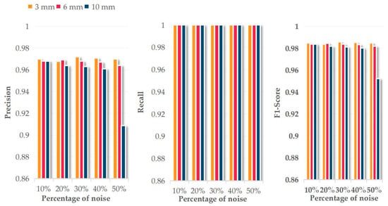
Figure 8.
The accuracy metrics of segmented points at different noise levels.
Figure 9 shows the accuracy metrics of segmented points from all methods at a noise level of 50% and s.d. of 10 mm on a Torus point cloud. The optimal results are achieved by the proposed method and the QTPS method, indicating the strong robustness of these two algorithms. In a comparison between the RG method and the RANSAC method, the former has poor robustness and eliminates the noise and its neighboring points, which results in lower Recall; the latter has stronger robustness but is easily affected by noise to produce over-fitting problems, resulting in lower precision. Similar to the RG, the PLINKAGE method presents weak robustness, and although it has a high precision value, a large number of noise points and their neighboring points are eliminated in the segmentation procedure.
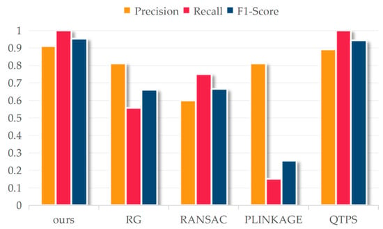
Figure 9.
The accuracy metrics of segmented points from all methods at a noise level of 50% and s.d. of 10 mm on a Torus point cloud.
4.3. Experiments on Real Point Cloud Datasets
Ten real datasets are used to test the proposed method, as shown in Figure 10 and Figure 11. The detailed data descriptions are listed in Table 2. The experimental datasets are airborne laser scanning point clouds acquired in Vaihingen, Germany, and Toronto, Canada [59].
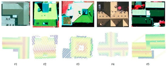
Figure 10.
Five point clouds and corresponding images in Vaihingen, Germany. The top row shows the images; the bottom row shows the point clouds.
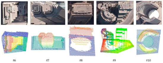
Figure 11.
Five point clouds and corresponding images in Toronto, Canada. The top row shows the images; the bottom row shows the point clouds.

Table 2.
Details of real datasets.
4.3.1. Qualitative Evaluations
To further evaluate the proposed method, contrastive analysis is performed with four state-of-the-art point cloud segmentation methods on ten typical datasets, as shown in Figure 12 and Figure 13. For datasets #1–#5, all buildings possess typical roof structures with low heights, no point clouds on the elevation, low noise, clear edges, and uniform point cloud density. All methods can segment the main shapes of the objects. The RG method relies on the angular difference between the normals of adjacent points, which enables it to detect most of the plane correctly. However, the normal vectors’ divergence at the planes’ intersections makes it difficult for the RG method to correctly assign the points there, as in dataset #4. In addition, the RG method is susceptible to noise and tends to form holes in the segmentation results, as in dataset #1. Compared with the RG method, the RANSAC method has stronger robustness, as can be seen in datasets #1 and #5. However, it is affected by the point cloud density; when the point cloud is dense, the complete structure can be extracted, and when the point cloud density is sparse, there will be unassigned points at the intersections, as can be seen in datasets #2 and #3. Similar to the RG method, the PLINKAGE method is sensitive to noise and tends to create holes in segmented planes. Furthermore, it often misses some points when processing shapes’ boundaries. QTPS uses a robust hierarchical clustering strategy based on a supervoxel, which can handle edges, especially when dealing with sparse point clouds. However, when dealing with a dense point cloud, there may be cross-border supervoxels, resulting in jaggedness at the edges, as can be seen in dataset #1. Our approach yields the optimal segmentation on all datasets, benefiting from the clustering on the Gaussian sphere that extracts the main shapes and the BIP optimization that reassigns outlier points to optimal shapes.
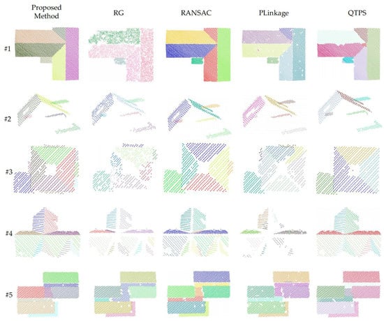
Figure 12.
Segmentation results on datasets #1 to #5.
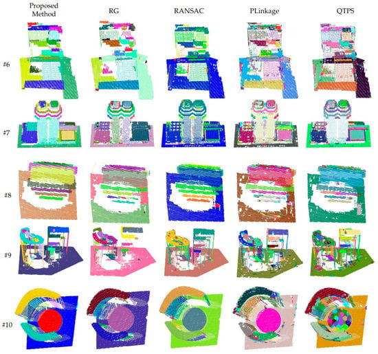
Figure 13.
Segmentation results on datasets #6 to #10.
For datasets #6–#10, the building structures are tall and complex, and point clouds exist on some elevations, with more noise and isolated points and a non-uniform point cloud density. Additionally, all methods can extract the objects’ primary structure. Among them, the PLINKAGE method, which is most affected by noise, generates the most significant number of holes and fragments. In contrast, the RG method is also affected by noise, but it chooses to denote the points that cannot participate in region growth as outliers. Although it generates voids, it does not classify these noises into new classes. The RANSAC and QTPS methods are robust to noise and generate fewer fragments, but these methods are more affected by isolated points. The former tends to create spurious facets, and the latter tends to cluster isolated points as fragments or form spurious facets with other isolated points due to the lack of means to deal with isolated points. Isolated points are not rare in ALS point clouds and often appear at locations with non-uniform density on the façade. The PLINKAGE method is prone to local convergence when dealing with these points, resulting in over-segmentation results. The Gaussian mapping used in this method is highly resistant to noise. This method eliminates isolated points or sparse points if they are far away from the primary shapes, i.e., if they are not linked to the primary shapes. In addition, all methods except the QTPS method have the ability to handle surfaces, as can be seen in dataset #10.
4.3.2. Quantitative Evaluations
Figure 14 shows the accuracy metrics of the proposed method and comparison methods on ten datasets. These metrics can reflect the quality of segmentation results in different aspects. For the three metrics of Precisionp, Recallp and F1-Scorep, the segmentation results are analyzed in terms of the point level. A lower Precisionp value indicates that the segmentation results in a large number of mis-segmented points. For example, in dataset #4, the RG method over-segments the same plane into multiple planes. In dataset #10, the QTPS method has difficulty handling the curved surface structure, causing the surface to be over-segmented into multiple small facets. A lower value of Recallp indicates that more points in the point cloud are not segmented and are finally considered outliers. For example, in dataset #4, the PLINKAGE method only succeeds in segmenting a small portion in each plane, and the other points in a large area are considered outliers.
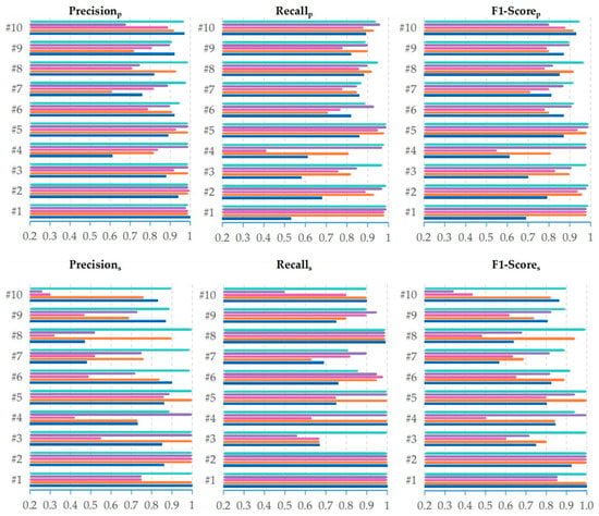
Figure 14.
The accuracy metrics of segmented results from five methods on real point cloud datasets.
Additionally, in dataset #1, the RG method similarly leads to more points being considered outliers due to the influence of noise. For the three metrics Precisions, Recalls, and F1-Scores, the segmentation results are analyzed in terms of the shape level. A lower value of Precisions indicates a large number of fragments in the segmentation results. For example, in dataset #10, QTPS uses fragmented facets to fit the surface, and in dataset #8, PLINKAGE generates a large number of fragments due to noise sensitivity. A lower value of Recalls indicates that more shapes in the point cloud are not segmented. For example, in dataset #3, QTPS fails to extract detailed structures around the building. F1-Score is the harmonic mean of Precision and Recall.
Although the RG method is noise-sensitive, it is known to have high precision. However, on datasets #7 and #8, Precisions is lower, but Precisionp is higher due to the fact that the main structures in the point cloud can be extracted. Still, more fragments are extracted due to the non-uniform density, which is especially evident in Figure 13. The segmentation of the RANSAC method generally has a high Recall value. In these experiments, the Recallp of most RANSAC results are higher than 0.8, and some of them are greater than 0.9. For dataset #3, due to its small number of structures, missing out on some detailed structures can cause a larger change in the Recalls value. For datasets #7 and #9, there are several cases where planes close to each other are identified as the same plane, which causes the Recalls value to decrease. Currently, the most popular methods are the RG and RANSAC methods. From the experimental results, it can be concluded that the former method has good precision and high efficiency. Still, the segmentation result is not complete when it comes to outlier reassignment, which is equivalent to the coarse extraction of this paper. Additionally, the lack of shape parameterization makes it difficult to apply to a subsequent 3D reconstruction and other requirements. The latter has higher Recall and can parameterize shapes, but the problem of spurious facets is challenging to avoid, which changes the spatial topology of the extracted shapes, making subsequent applications more difficult.
Similar to the proposed method, the PLINKAGE and QTPS methods also adopt a hierarchical clustering strategy. Most PLINKAGE method results have F1-Score values higher than 80% at the point level, while their F1 values at the shape level are lower than 70%. Because this algorithm has excellent shape detection capabilities, only the connection characteristics of local points are considered, which makes the algorithm vulnerable to noise and outlier points, so a large number of fragments are generated. QTPS has strong plane extraction capabilities, and, similar to the PLINKAGE method, the segmentation quality at the point level is much higher than that at the shape level. The main reason for this is that it is unable to recognize curved structures and is sensitive to isolated points. The PLINKAGE method uses Gaussian kernels to calculate the density of each point. Then, it chooses the point with the maximum local density as the center for clustering, which tends to produce over-segmentation on a point cloud with a non-uniform density. The QTPS method uses the strategy of supervoxel-based region growth, which optimizes the supervoxel to satisfy strict planarity and then extracts the accurate planar structure. From the experimental results, it can be concluded that this method does not eliminate isolated points. Too many isolated points can greatly reduce the quality of point cloud segmentation. In addition, a large number of supervoxels need to be optimized, which consumes much time.
Most of the accuracy metrics of the results from the proposed method are higher than 0.9, except for Recallp and Recalls from datasets #6 and #7. There are very sparse point clouds on the building façade of these two datasets, which make it difficult to form high-brightness point spots when mapped onto the Gaussian sphere, so this part cannot be identified in the main shape. Finally, the time consumption of each algorithm is shown in Figure 15. The time consumption of the RG, RANSAC, and PLINKAGE methods is proportional to the number of point clouds, and the time consumption of the QTPS method and the proposed method grows exponentially with the number of point clouds.
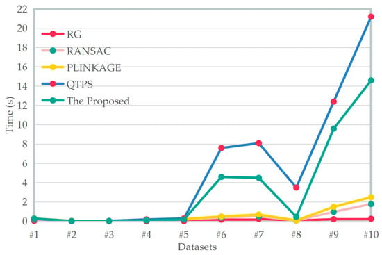
Figure 15.
The execution time (in seconds) of five methods on real point cloud datasets.
In conclusion, Gaussian mapping has strong robustness and is not affected by the non-uniform density of the point cloud. Thus, this paper introduces Gaussian mapping to complete the recognition of shape primitives. From the experimental results of synthetic datasets and real datasets, it can be found that various shape primitives can be identified intuitively on a Gaussian sphere with high accuracy. Then, this paper adopts an outlier reassignment strategy based on the BIP optimization model for the unrecognized outlier points. The optimization equation uses the minimum energy function and combines a variety of constraints to reassign the remaining points, performing complete multi-shape segmentation. The average F1-Scorep and F1-Scores of this method are 0.96 and 0.95, respectively. Nevertheless, the efficiency of this method is still lower than that of the RG and RANSAC methods, and further optimization is required in future research.
5. Conclusions
This paper proposes a two-stage automatic hierarchical clustering method for accurate building segmentation from LiDAR point clouds. In the first stage, we use Gaussian mapping to identify various types of geometric shapes composing the building and explicitly parameterize them to complete the point cloud’s coarse segmentation. In the second stage, we use the BIP optimization model to reassign the outlier points to complete the fine segmentation. Through experiments with synthetic and real datasets, it is proven that our method can complete the segmentation of common building shapes with high accuracy. Compared with other state-of-the-art methods, the segmentation results of the proposed method are significantly improved in terms of completeness and accuracy, proving its broad application prospects in 3D building reconstruction.
Author Contributions
Conceptualization, F.W. and G.Z.; methodology, F.W.; software, F.W. and J.X.; validation, B.F. and H.Y.; formal analysis, J.C., X.S. and B.Z.; writing—original draft preparation, F.W.; writing—review and editing, F.W. and J.X. All authors have read and agreed to the published version of the manuscript.
Funding
This research was funded by the Guangxi Natural Science Foundation (grant numbers 2021GXNSFBA220001 and 2022GXNSFBA035563) and the Open Fund of Guangxi Key Laboratory of Spatial Information and Geomatics (grant number 19-050-11-25).
Data Availability Statement
The synthetic datasets presented in this study are available upon request from the corresponding author. The real datasets are available at www.isprs.org/education/benchmarks/UrbanSemLab/Default.aspx, accessed on 14 January 2023.
Acknowledgments
The authors would like to thank Xiaohu Lu and Xianzhang Zhu for providing the source codes and executable programs for the experimental comparison and the reviewers for their constructive comments and suggestions.
Conflicts of Interest
The authors declare no conflict of interest.
References
- Zhou, G.; Zhou, X.; Song, Y.; Xie, D.; Wang, L.; Yan, G.; Hu, M.; Liu, B.; Shang, W.; Gong, C.; et al. Design of supercontinuum laser hyperspectral light detection and ranging (LiDAR) (SCLaHS LiDAR). Int. J. Remote Sens. 2021, 42, 3731–3755. [Google Scholar] [CrossRef]
- Chen, R.; Han, S.; Xu, J.; Su, H. Visibility-aware point-based multi-view stereo network. IEEE T Pattern. Anal. 2020, 43, 3695–3708. [Google Scholar] [CrossRef] [PubMed]
- Li, L.; Song, N.; Sun, F.; Liu, X.; Wang, R.; Yao, J.; Cao, S. Point2Roof: End-to-end 3D building roof modeling from airborne LiDAR point clouds. ISPRS J. Photogramm. 2022, 193, 17–28. [Google Scholar] [CrossRef]
- Huang, J.; Stoter, J.; Peters, R.; Nan, L. City3D: Large-Scale Building Reconstruction from Airborne LiDAR Point Clouds. Remote Sens. 2022, 14, 2254. [Google Scholar] [CrossRef]
- Li, Y.; Ibanez-Guzman, J. Lidar for Autonomous Driving: The Principles, Challenges, and Trends for Automotive Lidar and Perception Systems. IEEE Signal Proc. Mag. 2020, 37, 50–61. [Google Scholar] [CrossRef]
- Nwakanma, C.I.; Islam, F.B.; Maharani, M.P.; Lee, J.; Kim, D. Detection and Classification of Human Activity for Emergency Response in Smart Factory Shop Floor. Appl. Sci. 2021, 11, 3662. [Google Scholar] [CrossRef]
- Xu, B.; Chen, Z.; Zhu, Q.; Ge, X.; Huang, S.; Zhang, Y.; Liu, T.; Wu, D. Geometrical Segmentation of Multi-Shape Point Clouds Based on Adaptive Shape Prediction and Hybrid Voting RANSAC. Remote Sens. 2022, 14, 2024. [Google Scholar] [CrossRef]
- Xie, Y.; Tian, J.; Zhu, X.X. Linking Points with Labels in 3D: A Review of Point Cloud Semantic Segmentation. IEEE Geosci. Remote Sens. Mag. 2020, 8, 38–59. [Google Scholar] [CrossRef]
- Barnefske, E.; Sternberg, H. Evaluating the Quality of Semantic Segmented 3D Point Clouds. Remote Sens. 2022, 14, 446. [Google Scholar] [CrossRef]
- Liang, X.; Fu, Z.; Sun, C.; Hu, Y. MHIBS-Net: Multiscale hierarchical network for indoor building structure point clouds semantic segmentation. Int. J. Appl. Earth Obs. 2021, 102, 102449. [Google Scholar] [CrossRef]
- Wang, F.; Hu, H.; Ge, X.; Xu, B.; Zhong, R.; Ding, Y.; Xie, X.; Zhu, Q. Multientity Registration of Point Clouds for Dynamic Objects on Complex Floating Platform Using Object Silhouettes. IEEE Trans. Geosci. Remote Sens. 2021, 59, 769–783. [Google Scholar] [CrossRef]
- Sun, S.; Li, C.; Chee, P.W.; Paterson, A.H.; Jiang, Y.; Xu, R.; Robertson, J.S.; Adhikari, J.; Shehzad, T. Three-dimensional photogrammetric mapping of cotton bolls in situ based on point cloud segmentation and clustering. ISPRS J. Photogramm. 2020, 160, 195–207. [Google Scholar] [CrossRef]
- Nurunnabi, A.; Belton, D.; West, G. Robust Segmentation in Laser Scanning 3D Point Cloud Data. In Proceedings of the 2012 International Conference on Digital Image Computing Techniques and Applications (DICTA), Fremantle, Australia, 3–5 December 2012; pp. 1–8. [Google Scholar]
- Zhan, Q.; Liang, Y.; Xiao, Y. Color-based segmentation of point clouds. In Proceedings of the ISPRS Workshop Laserscanning ’09, Paris, France, 1–2 September 2009; pp. 248–252. [Google Scholar]
- Filin, S.; Pfeifer, N. Segmentation of airborne laser scanning data using a slope adaptive neighborhood. ISPRS J. Photogramm. 2006, 60, 71–80. [Google Scholar] [CrossRef]
- Vo, A.; Truong-Hong, L.; Laefer, D.F.; Bertolotto, M. Octree-based region growing for point cloud segmentation. ISPRS J. Photogramm. 2015, 104, 88–100. [Google Scholar] [CrossRef]
- Xu, Y.; Tong, X.; Stilla, U. Voxel-based representation of 3D point clouds: Methods, applications, and its potential use in the construction industry. Automat. Constr. 2021, 126, 103675. [Google Scholar] [CrossRef]
- Zhu, Q.; Wang, F.; Hu, H.; Ding, Y.; Xie, J.; Wang, W.; Zhong, R. Intact planar abstraction of buildings via global normal refinement from noisy oblique photogrammetric point clouds. ISPRS Int. J. Geo.-Inf. 2018, 7, 431. [Google Scholar] [CrossRef]
- Dong, Z.; Yang, B.; Hu, P.; Scherer, S. An efficient global energy optimization approach for robust 3D plane segmentation of point clouds. ISPRS J. Photogramm. 2018, 137, 112–133. [Google Scholar] [CrossRef]
- Ballard, D.H. Generalizing the Hough transform to detect arbitrary shapes. Pattern Recogn. 1981, 13, 111–122. [Google Scholar] [CrossRef]
- Fischler, M.A.; Bolles, R.C. Random sample consensus: A paradigm for model fitting with applications to image analysis and automated cartography. Commun. ACM 1981, 24, 381–395. [Google Scholar] [CrossRef]
- Xu, L.; Oja, E. Randomized Hough Transform (RHT): Basic Mechanisms, Algorithms, and Computational Complexities. CVGIP Image Underst. 1993, 57, 131–154. [Google Scholar] [CrossRef]
- Kiryati, N.; Eldar, Y.; Bruckstein, A.M. A probabilistic Hough transform. Pattern Recogn 1991, 24, 303–316. [Google Scholar] [CrossRef]
- Yla-Jaaski, A.; Kiryati, N. Adaptive termination of voting in the probabilistic circular Hough transform. IEEE Trans. Pattern Anal. 1994, 16, 911–915. [Google Scholar] [CrossRef]
- Galamhos, C.; Matas, J.; Kittler, J. Progressive probabilistic Hough transform for line detection. In Proceedings of the 1999 IEEE Computer Society Conference on Computer Vision and Pattern Recognition, Fort Collins, CO, USA, 23–25 June 1999; pp. 554–560. [Google Scholar]
- Widyaningrum, E.; Gorte, B.; Lindenbergh, R. Automatic Building Outline Extraction from ALS Point Clouds by Ordered Points Aided Hough Transform. Remote Sens. 2019, 11, 1727. [Google Scholar] [CrossRef]
- Romanengo, C.; Biasotti, S.; Falcidieno, B. Hough Transform for Detecting Space Curves in Digital 3D Models. J. Math. Imaging Vis. 2022, 64, 284–297. [Google Scholar] [CrossRef]
- Chen, D.; Zhang, L.; Mathiopoulos, P.T.; Huang, X. A Methodology for Automated Segmentation and Reconstruction of Urban 3-D Buildings from ALS Point Clouds. IEEE J. Stars 2014, 7, 4199–4217. [Google Scholar] [CrossRef]
- Xu, B.; Jiang, W.; Shan, J.; Zhang, J.; Li, L. Investigation on the weighted ransac approaches for building roof plane segmentation from lidar point clouds. Remote Sens. 2016, 8, 5. [Google Scholar] [CrossRef]
- Canaz Sevgen, S.; Karsli, F. An improved RANSAC algorithm for extracting roof planes from airborne lidar data. Photogramm. Rec. 2020, 35, 40–57. [Google Scholar] [CrossRef]
- Wang, F.; Zhou, G.; Hu, H.; Wang, Y.; Fu, B.; Li, S.; Xie, J. Reconstruction of LoD-2 Building Models Guided by Façade Structures from Oblique Photogrammetric Point Cloud. Remote Sens. 2023, 15, 400. [Google Scholar] [CrossRef]
- Liu, H.; Song, R.; Zhang, X.; Liu, H. Point cloud segmentation based on Euclidean clustering and multi-plane extraction in rugged field. Meas. Sci. Technol. 2021, 32, 95106. [Google Scholar] [CrossRef]
- Filin, S. Surface classification from airborne laser scanning data. Comput. Geosci. 2004, 30, 1033–1041. [Google Scholar] [CrossRef]
- Nurunnabi, A.; West, G.; Belton, D. Outlier detection and robust normal-curvature estimation in mobile laser scanning 3D point cloud data. Pattern Recogn. 2015, 48, 1404–1419. [Google Scholar] [CrossRef]
- Morsdorf, F.; Meier, E.; Kötz, B.; Itten, K.I.; Dobbertin, M.; Allgöwer, B. LIDAR-based geometric reconstruction of boreal type forest stands at single tree level for forest and wildland fire management. Remote Sens. Environ. 2004, 92, 353–362. [Google Scholar] [CrossRef]
- Xiao, W.; Zaforemska, A.; Smigaj, M.; Wang, Y.; Gaulton, R. Mean Shift Segmentation Assessment for Individual Forest Tree Delineation from Airborne Lidar Data. Remote Sens. 2019, 11, 1263. [Google Scholar] [CrossRef]
- Zhang, P.; Li, J.; Yang, X.; Zhu, H. Semi-automatic extraction of rock discontinuities from point clouds using the ISODATA clustering algorithm and deviation from mean elevation. Int. J. Rock Mech. Min. 2018, 110, 76–87. [Google Scholar] [CrossRef]
- Hu, C.; Pan, Z.; Zhong, T. Leaf and wood separation of poplar seedlings combining locally convex connected patches and K-means++ clustering from terrestrial laser scanning data. J. Appl. Remote Sens. 2020, 14, 18502. [Google Scholar] [CrossRef]
- Hou, J.; Zhang, A.; Qi, N. Density peak clustering based on relative density relationship. Pattern Recogn. 2020, 108, 107554. [Google Scholar] [CrossRef]
- Xu, X.; Luo, M.; Tan, Z.; Zhang, M.; Yang, H. Plane segmentation and fitting method of point clouds based on improved density clustering algorithm for laser radar. Infrared Phys. Technol. 2019, 96, 133–140. [Google Scholar] [CrossRef]
- Zhao, J.; Dong, Y.; Ma, S.; Liu, H.; Wei, S.; Zhang, R.; Chen, X.; Teodoro, A.C. An Automatic Density Clustering Segmentation Method for Laser Scanning Point Cloud Data of Buildings. Math. Probl. Eng. 2019, 2019, 3026758. [Google Scholar] [CrossRef]
- Chen, X.; Wu, H.; Lichti, D.; Han, X.; Ban, Y.; Li, P.; Deng, H. Extraction of indoor objects based on the exponential function density clustering model. Inf. Sci. 2022, 607, 1111–1135. [Google Scholar] [CrossRef]
- Wang, C.; Ji, M.; Wang, J.; Wen, W.; Li, T.; Sun, Y. An Improved DBSCAN Method for LiDAR Data Segmentation with Automatic Eps Estimation. Sensors 2019, 19, 172. [Google Scholar] [CrossRef]
- Chen, H.; Liang, M.; Liu, W.; Wang, W.; Liu, P.X. An approach to boundary detection for 3D point clouds based on DBSCAN clustering. Pattern Recogn. 2022, 124, 108431. [Google Scholar] [CrossRef]
- Yao, W.; Hinz, S.; Stilla, U. Object extraction based on 3D-segmentation of LiDAR data by combining mean shift with normalized cuts: Two examples from urban areas. In Proceedings of the 2009 Joint Urban Remote Sensing Event, Shanghai, China, 20–22 May 2009; pp. 1–6. [Google Scholar]
- Shahzad, M.; Zhu, X.X. Robust Reconstruction of Building Facades for Large Areas Using Spaceborne TomoSAR Point Clouds. IEEE Trans. Geosci. Remote 2015, 53, 752–769. [Google Scholar] [CrossRef]
- Dash, M.; Liu, H.; Scheuermann, P.; Tan, K.L. Fast hierarchical clustering and its validation. Data Knowl. Eng. 2003, 44, 109–138. [Google Scholar] [CrossRef]
- Xu, S.; Wang, R.; Wang, H.; Zheng, H. An Optimal Hierarchical Clustering Approach to Mobile LiDAR Point Clouds. IEEE Trans. Intell. Transp. 2020, 21, 2765–2776. [Google Scholar] [CrossRef]
- Jurado, J.M.; Cárdenas, J.L.; Ogayar, C.J.; Ortega, L.; Feito, F.R. Semantic segmentation of natural materials on a point cloud using spatial and multispectral features. Sensors 2020, 20, 2244. [Google Scholar] [CrossRef]
- Saxena, A.; Prasad, M.; Gupta, A.; Bharill, N.; Patel, O.P.; Tiwari, A.; Er, M.J.; Ding, W.; Lin, C. A review of clustering techniques and developments. Neurocomputing 2017, 267, 664–681. [Google Scholar] [CrossRef]
- Feng, C.; Taguchi, Y.; Kamat, V.R. Fast plane extraction in organized point clouds using agglomerative hierarchical clustering. In Proceedings of the 2014 IEEE International Conference on Robotics and Automation (ICRA), Hong Kong, China, 31 May–7 June 2014; pp. 6218–6225. [Google Scholar]
- Li, L.; Yao, J.; Tu, J.; Liu, X.; Li, Y.; Guo, L. Roof plane segmentation from airborne LiDAR data using hierarchical clustering and boundary relabeling. Remote Sens. 2020, 12, 1363. [Google Scholar] [CrossRef]
- Lu, X.; Yao, J.; Tu, J.; Li, K.; Li, L.; Liu, Y. Pairwise linkage for point cloud segmentation. ISPRS Ann. Photogramm. Remote Sens. Spat. Inf. Sci. 2016, 3, 201–208. [Google Scholar] [CrossRef]
- Kung, Y.; Huang, Y.; Chien, S. Efficient Surface Detection for Augmented Reality on 3D Point Clouds. In Proceedings of the 33rd Computer Graphics International, Heraklion, Greece, 28 June–1 July 2016; pp. 89–92. [Google Scholar]
- Zhang, C.; Zhang, K.; Ge, L.; Zou, K.; Wang, S.; Zhang, J.; Li, W. A method for organs classification and fruit counting on pomegranate trees based on multi-features fusion and support vector machine by 3D point cloud. Sci. Hortic. 2021, 278, 109791. [Google Scholar] [CrossRef]
- Schubert, E.; Sander, J.; Ester, M.; Kriegel, H.P.; Xu, X. DBSCAN revisited, revisited: Why and how you should (still) use DBSCAN. ACM Trans. Database Syst. 2017, 42, 1–21. [Google Scholar] [CrossRef]
- Schnabel, R.; Wahl, R.; Klein, R. Efficient RANSAC for Point-Cloud Shape Detection. Comput. Graph. Forum. 2007, 26, 214–226. [Google Scholar] [CrossRef]
- Zhu, X.; Liu, X.; Zhang, Y.; Wan, Y.; Duan, Y. Robust 3-D Plane Segmentation From Airborne Point Clouds Based on Quasi-A-Contrario Theory. IEEE J. Stars 2021, 14, 7133–7147. [Google Scholar] [CrossRef]
- Rottensteiner, F.; Sohn, G.; Jung, J.; Gerke, M.; Baillard, C.; Benitez, S.; Breitkopf, U. The ISPRS Benchmark on urban object classification and 3D building reconstruction. ISPRS Ann. Photogramm. Remote Sens. Spat. Inf. Sci. 2012, I-3, 293–298. [Google Scholar] [CrossRef]
Disclaimer/Publisher’s Note: The statements, opinions and data contained in all publications are solely those of the individual author(s) and contributor(s) and not of MDPI and/or the editor(s). MDPI and/or the editor(s) disclaim responsibility for any injury to people or property resulting from any ideas, methods, instructions or products referred to in the content. |
© 2023 by the authors. Licensee MDPI, Basel, Switzerland. This article is an open access article distributed under the terms and conditions of the Creative Commons Attribution (CC BY) license (https://creativecommons.org/licenses/by/4.0/).