A Double-Adaptive Adjustment Algorithm for Ionospheric Tomography

Abstract

A double-adaptive adjustment algorithm (DAAA) is proposed to reconstruct three-dimensional ionospheric electron density (IED) distribution. In the DAAA method, the relaxation factor of the multiplicative algebraic reconstruction technique (MART) is first adaptively adjusted by introducing adaptive MART (AMART). To avoid the voxels without any rays traversing them becoming dependent on the initial IED values, smoothing constraints are generally imposed on the adaptive multiplicative algebraic reconstruction technique (AMART). In general, the elements of the smoothing matrices are invariant in the iterative process. They affect the accuracy and efficiency of the IED inversion. To overcome the above limitation, the adaptive adjustments of the constrained matrix elements are subsequently carried out. Both numerical simulation and actual global navigation satellite system (GNSS) experimental results validate that the accuracy and efficiency of ionospheric tomography have been improved by the DAAA method. Finally, the new algorithm is applied to reconstruct the three-dimensional structure of the ionosphere during different geomagnetic activities. The comparisons show that the vertical profiles of the DAAA method are in agreement with those recorded from the ionosonde, and the inverted vertical total electron content (VTEC) of the DAAA method also agrees with the ionospheric products of center for orbit determination in Europe (CODE) during geomagnetic quiet and geomagnetic storms. The comparisons confirm the reliability and superiority of the DAAA method.

1. Introduction

The ionosphere is an important component of the earth’s atmosphere that affects the propagation of GNSS signals [1,2]. Therefore, it is necessary to know the temporal-spatial variation of the ionosphere to improve the accuracy of ionospheric delay correction. Vertical total electron content (VTEC) is a key ionospheric parameter, which can be obtained by using thin layer hypothetical ionospheric models. However, the VTEC only describes the two-dimensional variations of the ionosphere in the horizontal section [3,4]. The advent of GNSS-based ionospheric tomography techniques provide a new means of ionospheric sounding, which attracts the attention of many scholars since it can reconstruct three-dimensional ionospheric structures [5,6,7,8,9,10,11,12]. At present, the theoretical and algorithmic investigations of these techniques are the focus of ionospheric tomography. The main difficulty surrounding these techniques is that the IED reconstruction is usually an ill-posed problem due to insufficient input data and uneven distribution of ground GNSS observation stations [13,14,15,16,17,18]. The ill-posed nature of this problem can cause large errors in approximate solutions even if the input data have only arbitrary, small errors. To solve the above problem, appropriate algorithms need to be studied. In the past years, many inversion algorithms have been released that attempt to solve the ill-posed nature of IED tomographic reconstruction. On the whole, the methods can be divided into two categories: iterative algorithms and non-iterative algorithms [2]. SVD is one non-iterative algorithm [19,20], and its efficiency is poor since the coefficient matrix of the tomographic system is usually large and sparse. It is not conducive to obtaining high temporal-spatial resolution IED images. Multiplicative and non-multiplicative algebraic reconstruction techniques (MART and ART) are the two typical methods in iterative algorithms [21,22]. They can reconstruct high resolution IED images from either very few or very limited views. However, ART performs iterative operations in the form of addition, which results in the IED values of some voxels being negative after iterative convergence [23]. It is not consistent with the fact that an IED value is usually positive. MART can ensure the positive inversion result since it performs iterative operation in the form of multiplication. However, the relaxation factor of MART retains invariants in the iterative process [24], which impacts the algorithm’s accuracy and computational efficiency. To overcome the limitations of MART, adaptive adjustment of the relaxation factor is first carried out in the DAAA method. Considering the dependence of the voxels without any rays traversing them on the initial IED values, an adaptive smoothing constraint is subsequently imposed on the tomographic system. To validate the feasibility and superiority of the double-adaptive adjustment algorithm, a numerical simulation is carried out, and the DAAA method is successfully applied to reconstruct three-dimensional IED distributions under quiet geomagnetic conditions and disturbed geomagnetic conditions. Finally, the reconstructed profiles of the DAAA method are compared with those obtained from the ionosonde data of Wuhan station.

2. Methods

Ionospheric tomography techniques use the input slant TEC (STEC) data to reconstruct IED distributions. The relationship between IED and STEC can be described using the following equation:

$$y={\displaystyle {\int }_{l}N\left(s\right)}ds$$

(1)

where y is the input STEC data; l represents the GNSS signal propagation path; and $N(s)$ is the IED. To simplify the calculation, the imaging region is discretized into a group of voxels, and the IED value of each voxel is assumed to be a constant in the selected time period. Then Equation (1) can be simplified as:

$$y_i={\displaystyle \sum _{j=1}^n{A}_{ij}{x}_j}i=1,2,\cdots ,m$$

(2)

Considering the discretization error and GNSS observation noise, Equation (2) can generally be written in a simple matrix notation as:

$$Y_{m\times 1}=A_{m\times n}{X}_{n\times 1}+E_{m\times 1}$$

(3)

where n is the number of the voxels; m is the number of STEC data; Y is a column vector that constitutes the input data; A is the sparse coefficient matrix; X is the IED vector; and E is error vector, which includes the discretized error and GNSS observation noise.

MART is a classical iterative algorithm of GNSS-based ionospheric tomography, and it has been widely used in the tomographic inversion of IED. The iteration is performed to improve the initial IED estimation that can be obtained from an empirical ionospheric model such as NeQuick. It is defined as a round of iterations when all input STEC data participate in an iteration. MART is an optimization algorithm based on the maximum entropy principle. It can be formulated as:

$$\left.\begin{array}{l}{x}_j^{(p+1)}=x_j^{(p)}{\left(\frac{y_i}{\langle a_i,x^{\left(p\right)}\rangle }\right)}^u\\ u=\frac{\lambda \cdot a_{ij}}{‖a‖}\end{array}\right\}$$

(4)

where $x_j^{(p)}$ is the pth iterative IED value of the jth voxel; $a_i$ is the ith row vector of matrix A; $\lambda$ is the relaxation factor, which is constant in the iterative process; and $u$ is the relaxation parameter that depends on the intercept value. The MART algorithm has fast iteration speed, and it can ensure that the inversion result is positive since MART improves the results using multiplication.

Equation (4) shows that the determination of the relaxation parameter $u$ is crucial for the MART method. Quick determination of the relaxation parameter can improve the accuracy and efficiency of IED reconstruction. The error allocation of the MART method is completely dependent on the intercept $a_{ij}$, and will amplify the error. In addition, the relaxation parameter only depends on the relaxation factor $\lambda$ since the vector $a_i$ does not vary with the iterative process of each round. The role of the relaxation factor $\lambda$ is to regulate the accuracy and the smoothness of the tomographic results. The larger relaxation factor makes the inversion results smoother. This means that the local variation characteristics of the ionosphere will be masked. However, the IED inversion will be affected by noise interference when the relaxation factor is too small.

To accelerate the iterative speed and improve the accuracy of IED tomographic reconstruction, it is necessary to improve the relaxation parameter. Zhao et al. has proposed the AMART [24], which adaptively adjusts the relaxation parameters according to the IED results of its last round of iterations. The AMART allocates the iterative difference using a more reasonable approach. Considering the advantages of the AMART method, it is introduced to perform the first adaptive adjustment of the relaxation parameter in this study. The AMART is as follows:

$$\left.\begin{array}{l}{x}_j^{(p+1)}=x_j^{(p)}{\left(\frac{y_i}{〈a_i,x^{(p)}〉}\right)}^u\\ u=\frac{{\lambda }_j^{(p)}{a}_{ij}{x}_j^{(p)}}{\sqrt{{\displaystyle \sum _{j=1}^n{\left(a_{ij}{x}_j^{(p)}\right)}^2}}}\\ {\lambda }_j^{(p)}=\frac{x_j^{(p)}}{N}\\ N>\max \left(x_j^{(p)}\right)\end{array}\right\}$$

(5)

where N is a constant; $x_j^{(p)}$ represents the pth iteration IED value of the jth voxel, and ${\lambda }_j^{(p)}$ is the pth iteration relaxation factor of the jth voxel. Equation (5) shows that the relaxation factor $\lambda$ and the relaxation parameter $u$ can be adjusted by using the iterative results of each round of iterations.

According to Equation (5), the AMART only improves the initial iterative values of the voxels with GNSS rays traversing them. In the actual inversion process, some voxels do not have any observation information. Their final results are the same as the initial IED values obtained from the empirical ionospheric model, which can only reflect the average ionospheric effect. The accuracy of IED initial values is usually low. To avoid the voxels without any rays traversing them becoming dependent on the initial iterative values, smoothing constraints are usually imposed on the iterative algorithms. However, the elements of the constrained matrix are usually fixed in each round of iterations [14,16], which affects the efficiency and accuracy of IED inversion to a certain extent. Considering the IED variation after each round of iterations, the elements of the constrained matrix can be adaptively adjusted according to the iterative results of the last round. In this work, the Gauss weighting function is introduced to construct the adaptively adjusted constraint matrix. In general, the constraint equation is given as:

$$h_1{x}_1+\dots +h_{d-1}{x}_{d-1}-x_d+h_{d+1}{x}_{d+1}+\dots +h_n{x}_n=0$$

(6)

For the proposed DAAA method, the weighting coefficient h_i can be expressed as:

$$h_j^{(p+1)}=\frac{e^{-{\left(B_{cd}^{(p)}\right)}^2/2{\sigma }^2}}{{\displaystyle \sum _{c_1=1}^{ne}{\displaystyle \sum _{d_1=1}^{nn}{e}^{-{\left(B_{c_{{}_1}{d}_{{}_1}}^{(p)}\right)}^2/2{\sigma }^2}}}}$$

(7)

In Equation (7)

$$B_{cd}^{\left(p\right)}=D_{cd}\times \frac{x_d^{\left(p\right)}}{x_c^{\left(p\right)}}$$

(8)

$$B_{c_1{d}_1}^{\left(p\right)}=D_{c_1{d}_1}\times \frac{x_{d_1}^{\left(p\right)}}{x_{c_1}^{\left(p\right)}}$$

(9)

where $ne$ and $nr$ are the number of voxels in the longitude and latitude directions, respectively; $D_{cd}$ is the distance between the cth voxel and the dth voxel; and $\sigma$ is the smoothing operator.

According to Equation (7), the horizontal constraint matrix is written as:

$$H=diag\left(H_1,H_2,\dots ,H_q\right)$$

(10)

where $H_q$ is the coefficient matrix of the qth layer of the reconstructed region. The horizontal constraint matrix can be described as:

$$HX=0$$

(11)

In the altitudinal direction, the IED variation is usually considered to be smooth and continuous. The prior IED profile information is used to establish the vertical constraint equation. In this study, the prior profile information is obtained from the IRI 2016 model. The IED of the adjacent voxels satisfies the following approximate ratio relationship:

$$\left[1-x_{k,j}^{(0)}/x_{k+1,j}^{(0)}\right]\left[\begin{array}{c}{x}_{k,j}^{(p)}\\ x_{k+1,j}^{(p)}\end{array}\right]=0$$

(12)

where $x_{k,j}^{(0)}$ is the vertical prior IED information of the jth voxel in the kth layer; and $x_{k,j}^{(p)}$ is the computed IED value of the jth voxel in the kth layer after the pth round iteration. According to Equation (12), the adaptive vertical constraint matrix $V$ can be created using the following expression:

$$VX=0$$

(13)

Combining Equation (3) with Equations (10) and (13), the following equations can be obtained:

$$\left[\begin{array}{c}Y\\ 0\\ 0\end{array}\right]=\left[\begin{array}{l}A\\ H\\ V\end{array}\right]X+E$$

(14)

3. Numerical Test of the New Algorithm

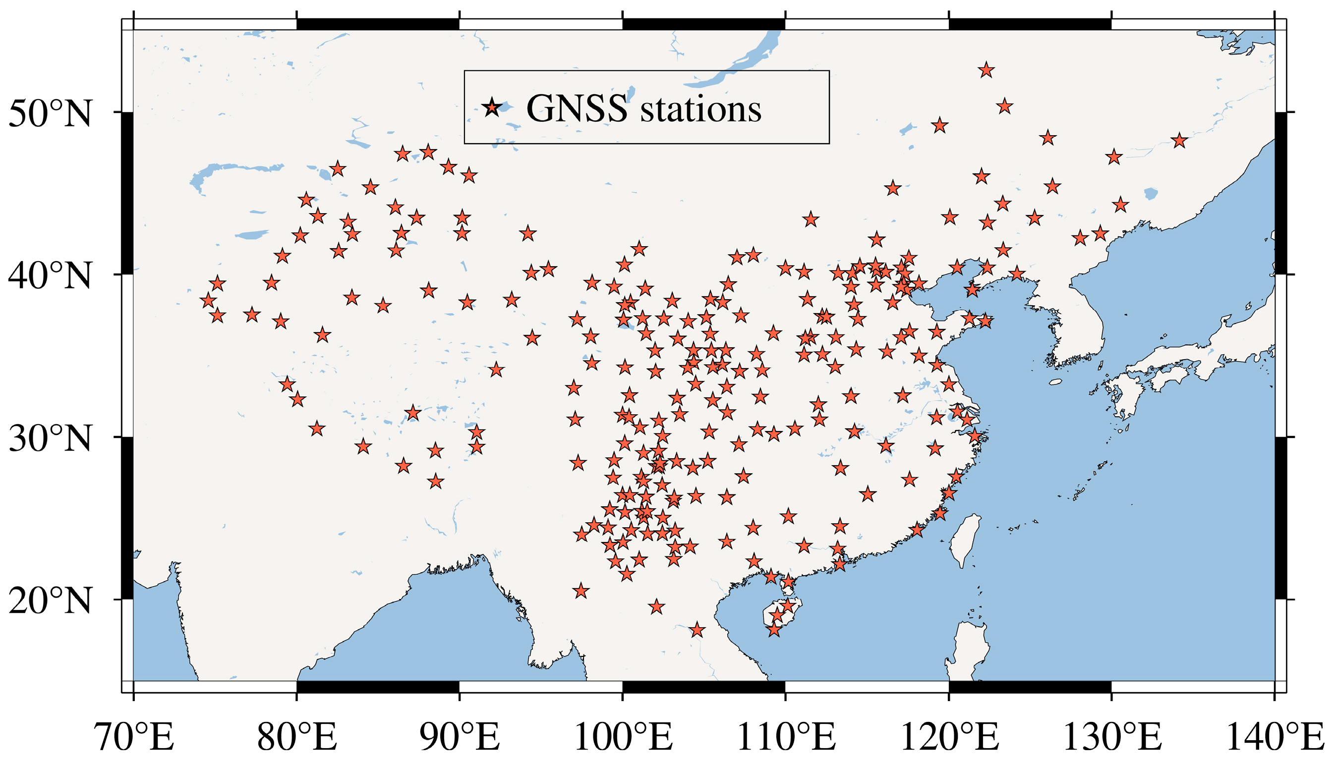
To test the reliability and superiority of the DAAA method proposed in this study, a numerical simulation scheme is first designed. In this simulation test, the latitude range varies from 10 °N to 55 °N, and the longitudinal range varies from 70 °E to 140 °E. In height, the range varies from 100 km to 1000 km. The discretized intervals are 0.5° and 1° in the latitudinal and longitudinal directions, respectively, and the altitudinal interval is 30 km. To perform the IED inversion, the geographical coordinates of 245 stations of the Crustal Movement Observation Network of China (CMONOC) are used to construct the coefficient matrix of the tomographic system. The geographical locations of the 245 GNSS stations are shown in Figure 1.

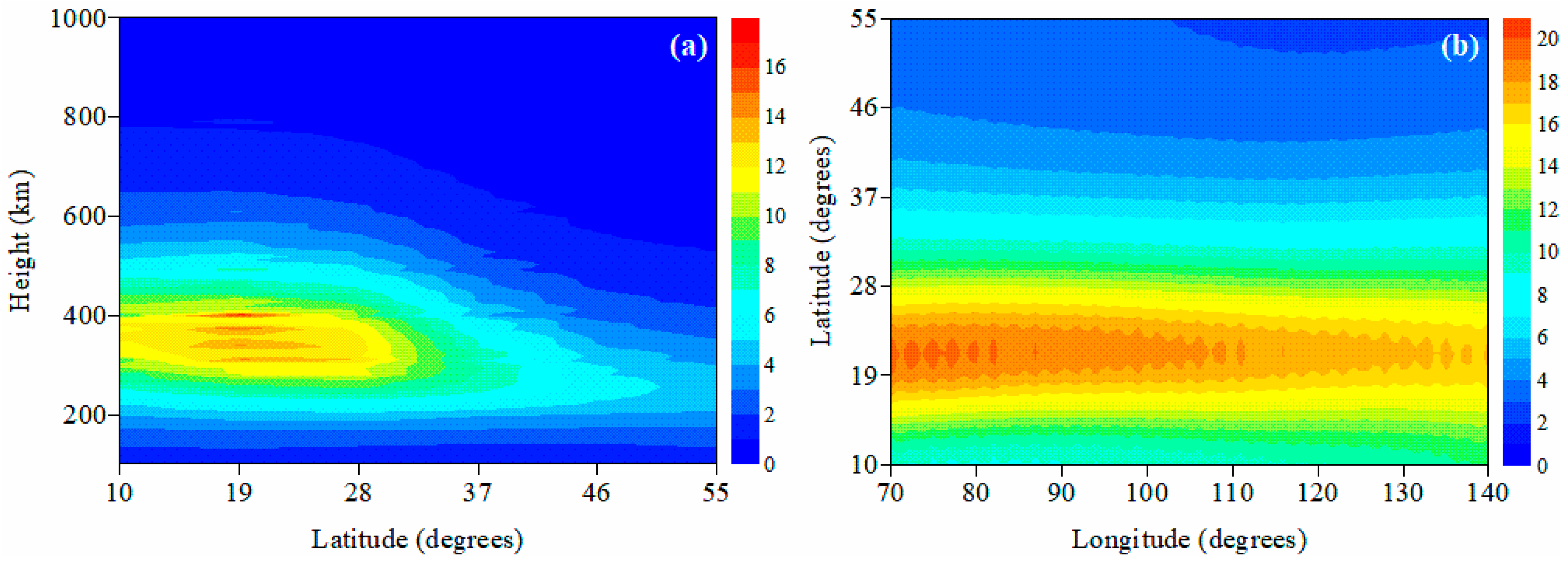
Considering the quiet geomagnetic activity, the selected time is 14:00UT on 15 August 2003. To run the DAAA method, it is necessary to obtain the initial IED value. In this study, the initial IED values are obtained from the NeQuick model to distinguish them from the subsequent true IED values. Figure 2 shows the two-dimensional images of the initial IED distributions in the different cross-sections. However, the true IED values are simulated using the IRI 2016 model in this study.

To evaluate the advantages of the DAAA over the MART and AMART, the mean absolute error (MAE) and the root mean square error (RMSE) of the three algorithms can be computed by using Equations (15) and (16), respectively.

$$\mathrm{MAE}={\displaystyle \sum _{j=1}^n\left|x_j^{true}-x_j^{tomo}\right|/n}$$

(15)

$$\mathrm{RMSE}=\sqrt{{\displaystyle \sum _{j=1}^n{\left(x_j^{true}-x_j^{tomo}\right)}^2}/n}$$

(16)

where $x_j^{true}$ is the simulated true IED value of the jth voxel using IRI 2016, and $x_j^{tomo}$ represents the tomographic result of the three algorithms.

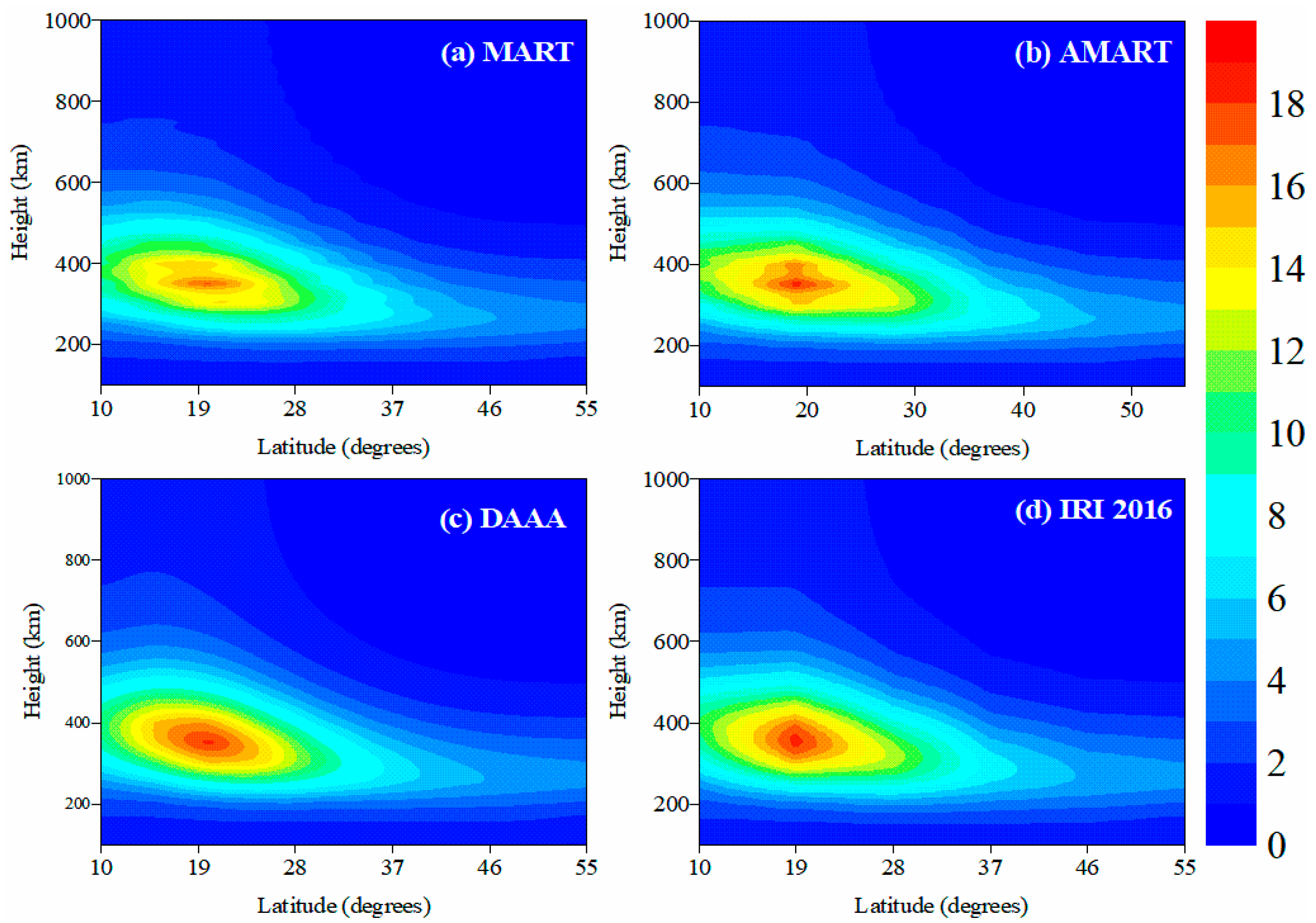
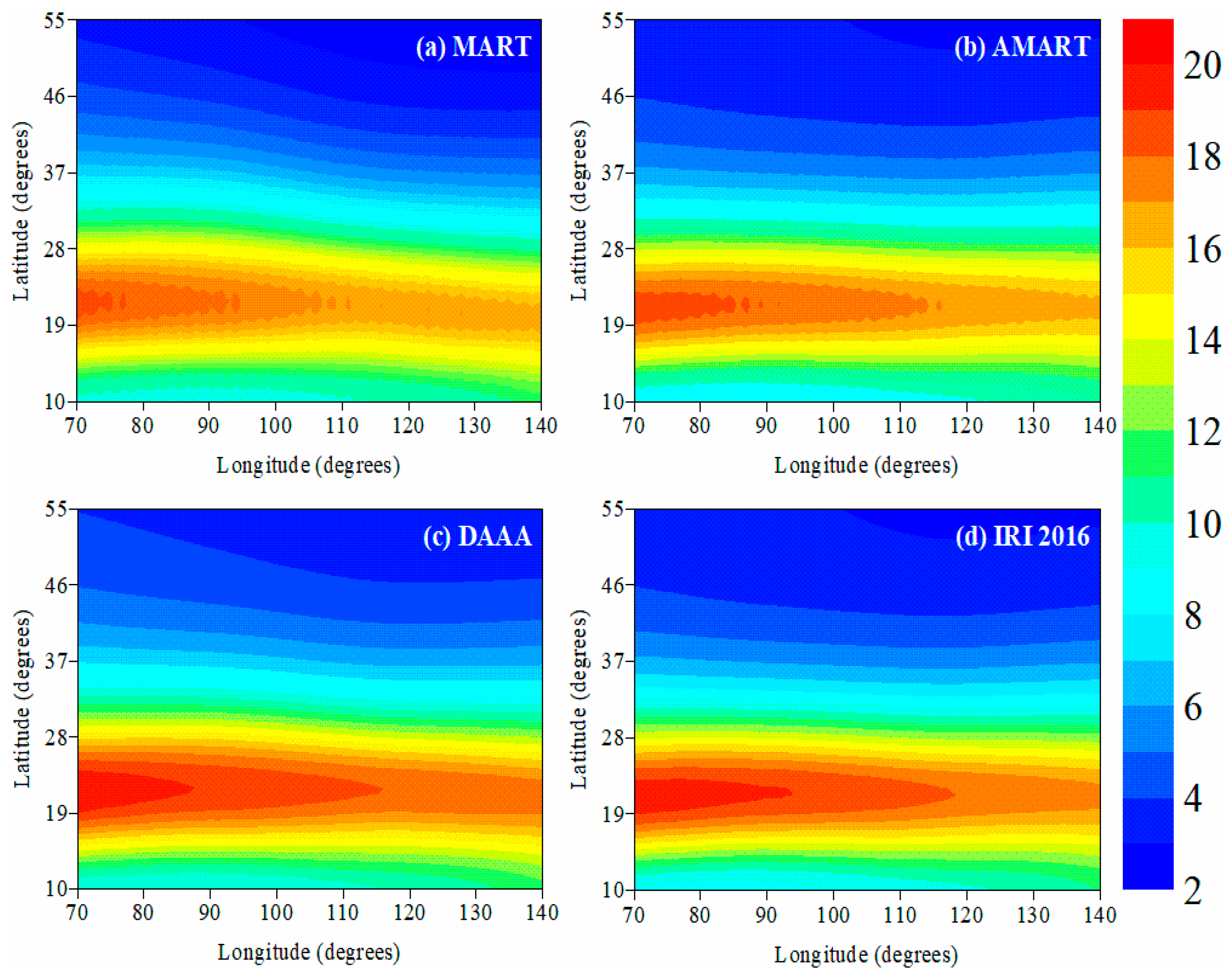
Figure 3 and Figure 4 compare the reconstructed images of three algorithms with the true IED values obtained from IRI 2016 along the longitudinal chain of 114°E and the altitudinal chain of 350 km, respectively. The comparisons show that the reconstructed results of the DAAA are closer to the true IED values than those of the MART and the AMART, and the imaging resolutions of the MART and the AMART are low.

Table 1. The statistics of the reconstructed error and the iterative round numbers of the three algorithms. The unit of the reconstructed error is 10¹¹ el/m³.

Methods	MART	AMART	DAAA
Maximum absolute error	5.16	3.87	0.89
MAE	2.87	1.55	0.23
RMSE	0.38	0.10	0.05
Iterative round numbers	28	17	11

gives the statistics of the reconstructed errors and iterative round numbers of the three algorithms. The statistics shows that the accuracy and the efficiency of IED reconstruction can be improved when the relaxation parameter is adaptively adjusted by the AMART. Subsequently, the accuracy and the efficiency are further improved when the adaptive smoothing constraints are imposed on the AMART by the DAAA. The simulated results validate that the reliability and the superiority of the DAAA over the AMART and the MART.

4. Real Experiment Based on Actual GNSS Observation

To further test the DAAA method, the actual GNSS observation data of CMONOC is used to reconstruct the three-dimensional IED images in China. Considering the quiet geomagnetic activity, the selected observation day is 3 September 2018 in this study, and the sample interval of GNSS data is 30 s. The diurnal variations of the ionosphere over China are studied.

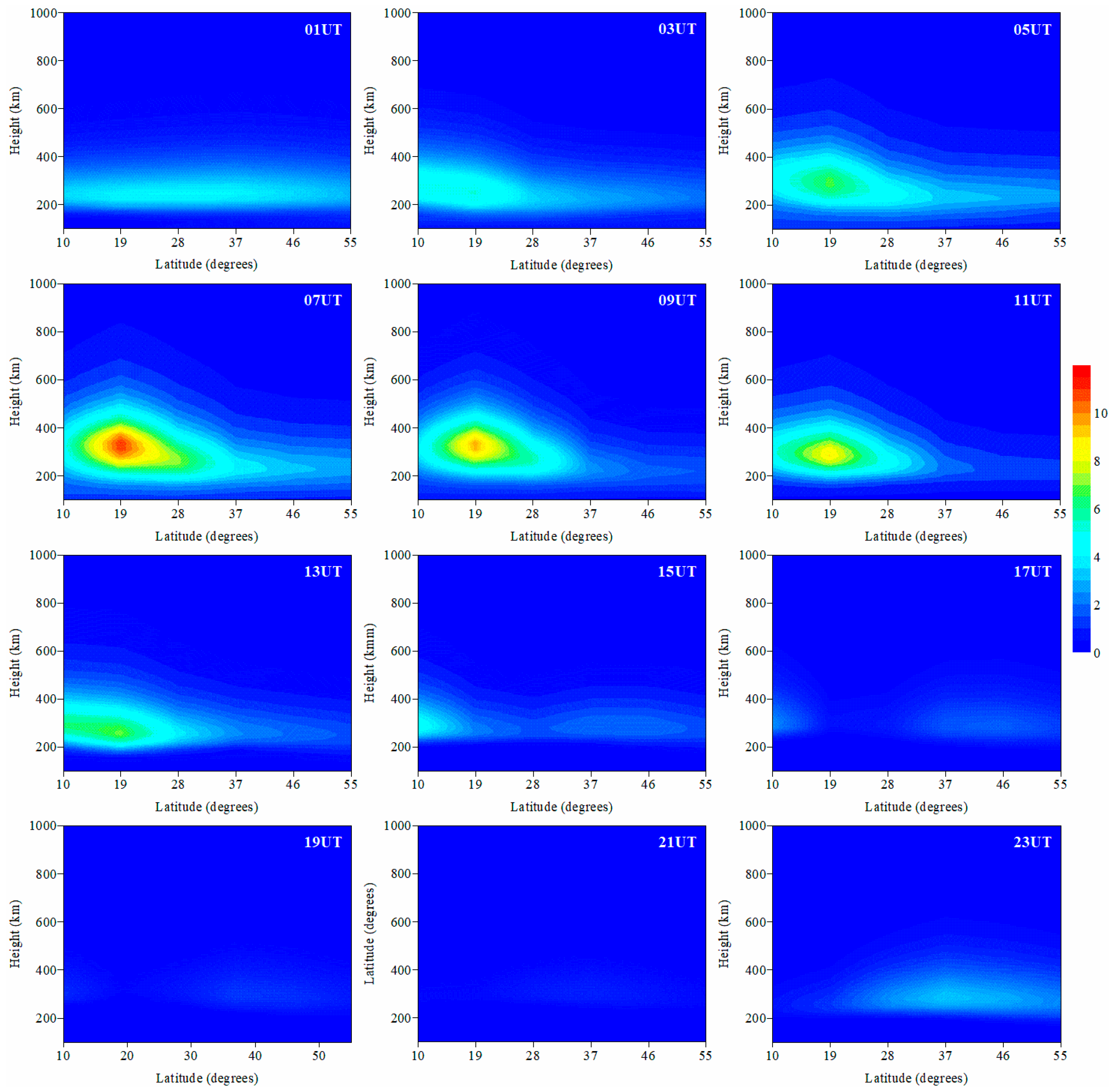
Figure 5 illustrates the time-series variations of the IED along the longitudinal chain of 114°E. The reconstructed images show that the IED values are the highest over time. The IED values reach their maximum at 07:00UT, and then the IED values begin to decrease. At 21:00UT, the IED value decreases to its lowest point. Subsequently, the IED values start to increase again. Meanwhile, Figure 5 shows that the equatorial anomaly core, with little inclination, is formed at 05:00UT and disappears at 11:00UT. On the whole, this experiment indicates that the IED values in northern China are generally smaller than those in southern China. This phenomenon demonstrates that the IED variations are closely related to the latitude.

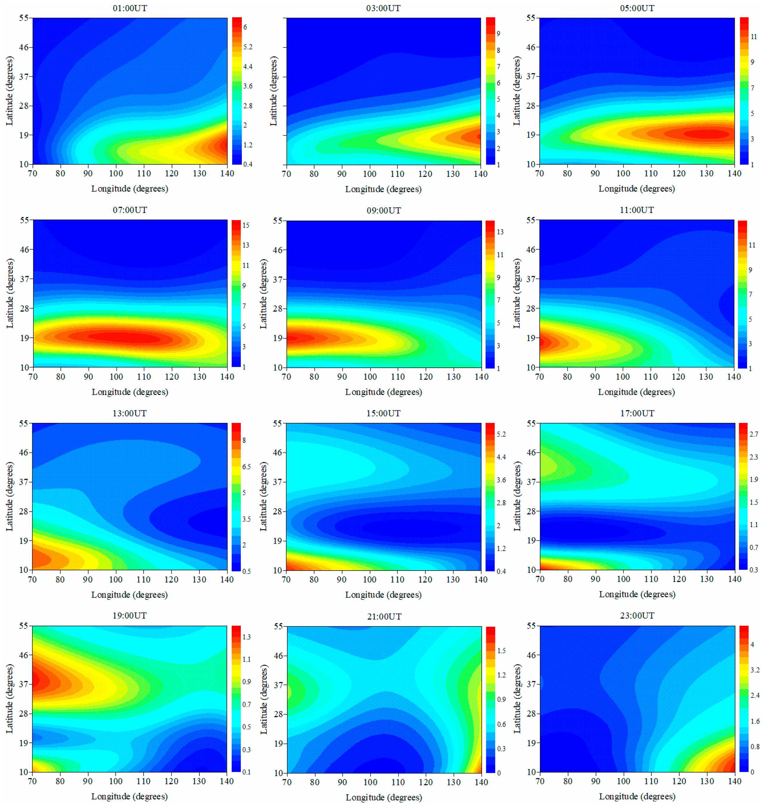
Figure 6 gives the diurnal variations of the IED at the altitude of 350 km. The subgraphs show that the IED values in eastern China are higher than those in western China between 01:00UT and 05:00UT. Subsequently, the IED in western China starts to increase as time elapses. Finally, the IED values in eastern China are lower than those in western China between 09:00UT and 19:00UT. Figure 6 also shows that the IED values first varies from small to large, and then the value varies from large to small as the earth rotates from west to east.

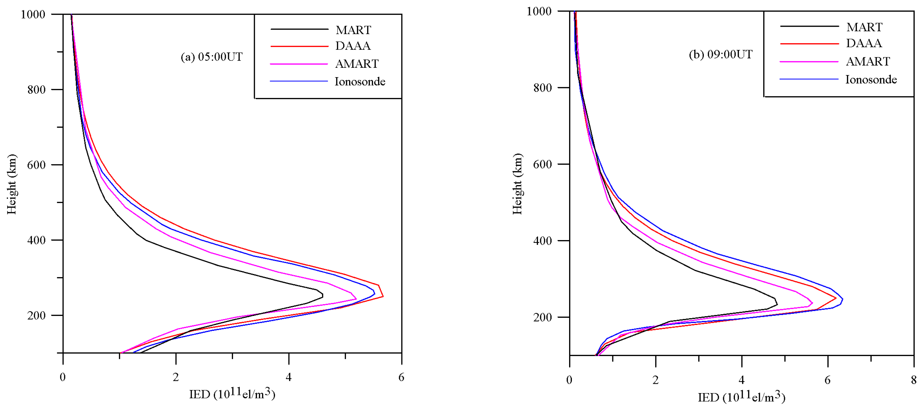
Figure 7 compares the reconstructed IED profiles of three algorithms at 05:00UT and 09:00UT with those recorded by the ionosonde station located in Wuhan. The comparisons show that the reconstructed IED profiles of the DAAA method are in agreement with those obtained from the ionosonde station. This comparison validates that the reconstructed results by the DAAA are more accurate than those of the MART and the AMART methods.

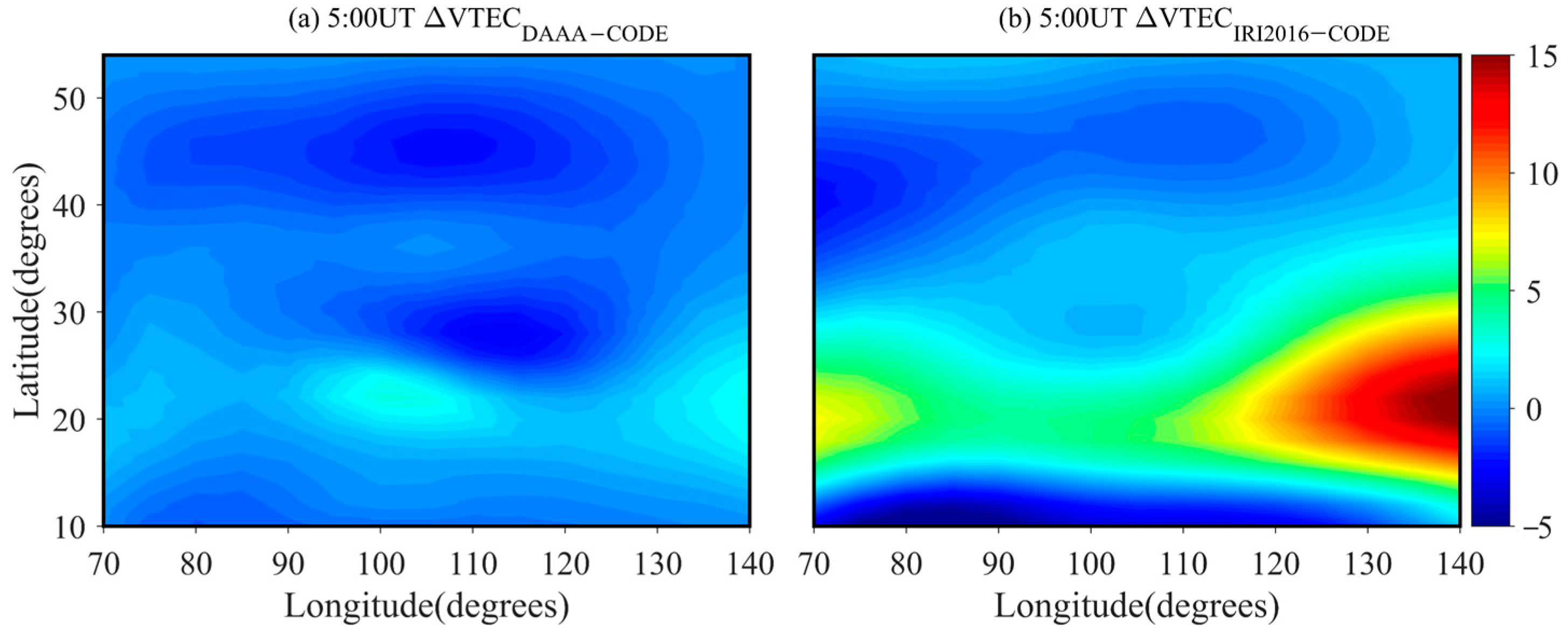
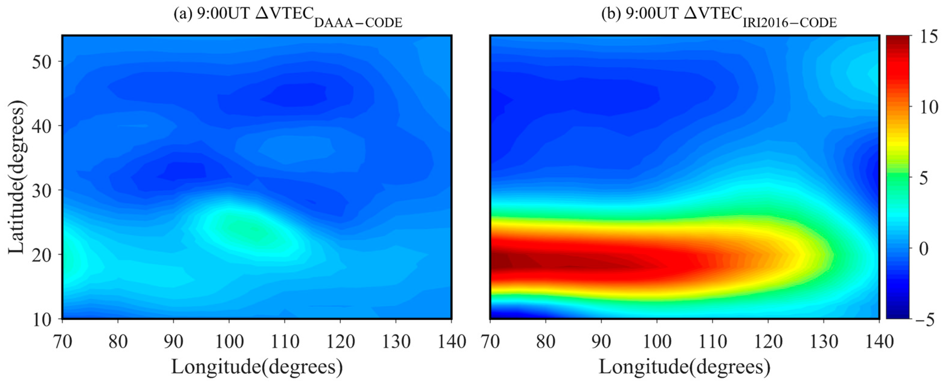
Using the IED values inverted from the DAAA method and the IRI 2016 model, the vertical TEC (VTEC) can be computed. Subsequently, the differential VTEC values between the inversion results and the ionospheric VTEC products of center for orbit determination in Europe (CODE) can be obtained. Figure 8 and Figure 9 show the differential VTEC images at 5:00UT and 9:00UT, respectively. Figure 8 and Figure 9 show that there is a significant deviation between the VTEC values calculated by the IRI 2016 model and the products released by CODE. The maximum of the differential VTEC amounts to 15TECU. The reason for this deviation is that the IRI 2016 model reflects the average variation effect of the ionosphere, so the inverted VTEC accuracy is therefore low. At 5:00 and 9:00UT, the maximum differential VTEC occurs in eastern China and the western China, respectively. However, the accuracy of the VTEC inverted by the DAAA method has been significantly improved, and the maximum VTEC error is less than 3TECU due to the DAAA using the real GNSS data to reconstruct the IED distribution. This validates that the inverted VTEC of the DAAA method is consistent with the products released by CODE. The comparisons further validate the reliability and superiority of the proposed DAAA method in this study.

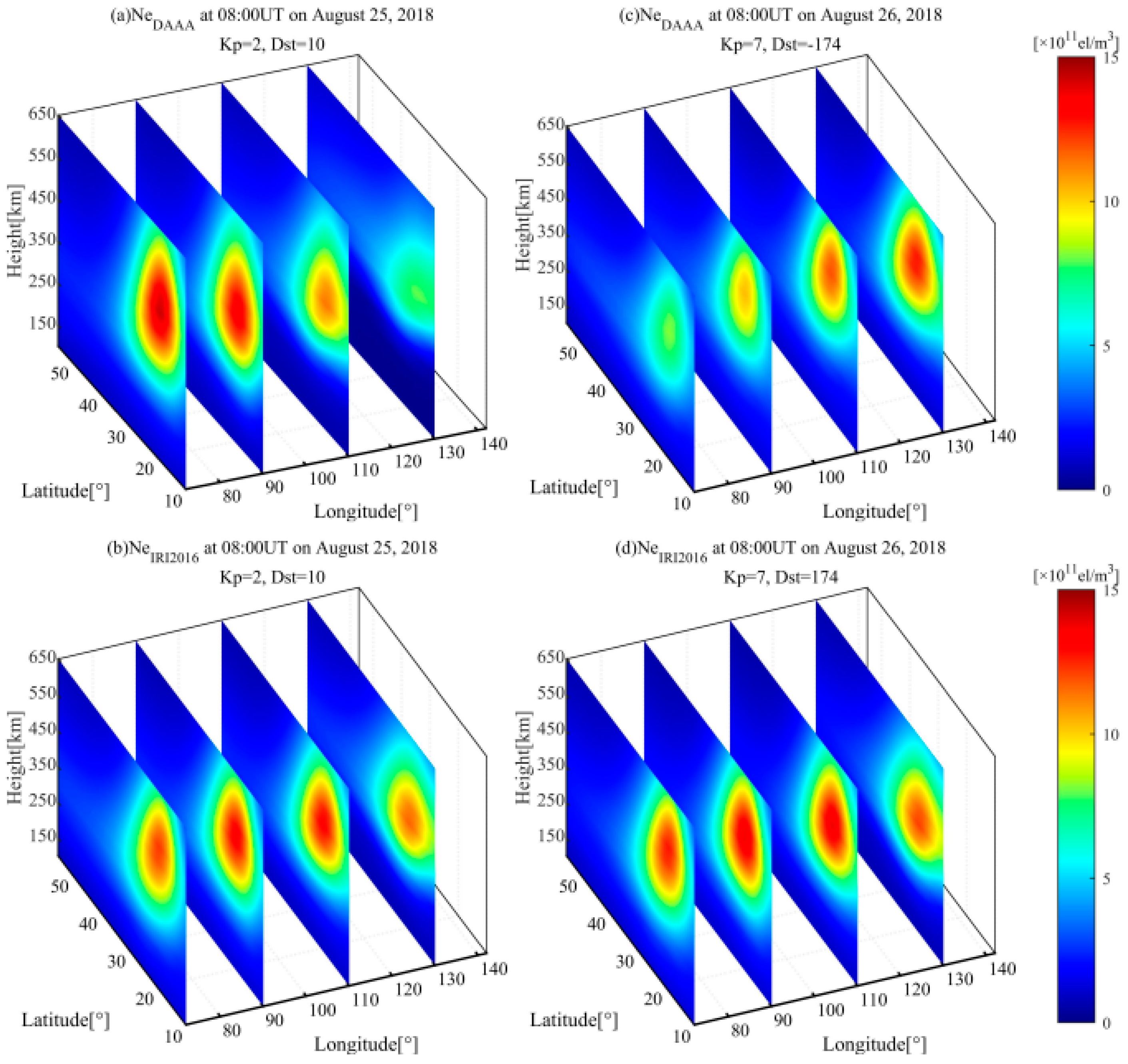
To verify the applicability of the DAAA method during geomagnetic storms, it is necessary to reconstruct the IED distribution during the magnetic storm using the new algorithm. In this study, the selected strong geomagnetic storm event occurred on 26 August 2018. The Kp index reached 7+ at 8:00UT. Using the dual-frequency GNSS observations of CMONOC, three-dimensional IED images are reconstructed by the DAAA. The reconstructed imaging is plotted in Figure 10c. Considering the quiet ionospheric activity at 08:00UT on 25 August 2018, the IED distribution is also reconstructed to compare with that during the geomagnetic storm. The reconstructed result is shown in Figure 10a. Comparing Figure 10c with Figure 10a, it can be seen that the IED values on the day of the storm evidently decrease in western China, exhibiting the negative storm phase effect. However, the positive storm phase effect occurs in eastern China. Figure 10b,d illustrate the three-dimensional IED distributions obtained from the IRI 2016 model during the selected geomagnetic quiet time and the geomagnetic storm time, respectively. Comparing the reconstructed images of the DAAA with the corresponding images obtained from IRI 2016 model shows that the IED values increase in western China during the geomagnetic quiet period. However, the IED values decrease in eastern China. During the occurrence of the geomagnetic storm, the IED variation is opposite to that in the geomagnetic quiet state. Meanwhile, Figure 10a shows that the IED values gradually decrease from west to east in a geomagnetically quiet state. Figure 10c shows that the IED values increase from west to east when in a geomagnetically disturbed state.

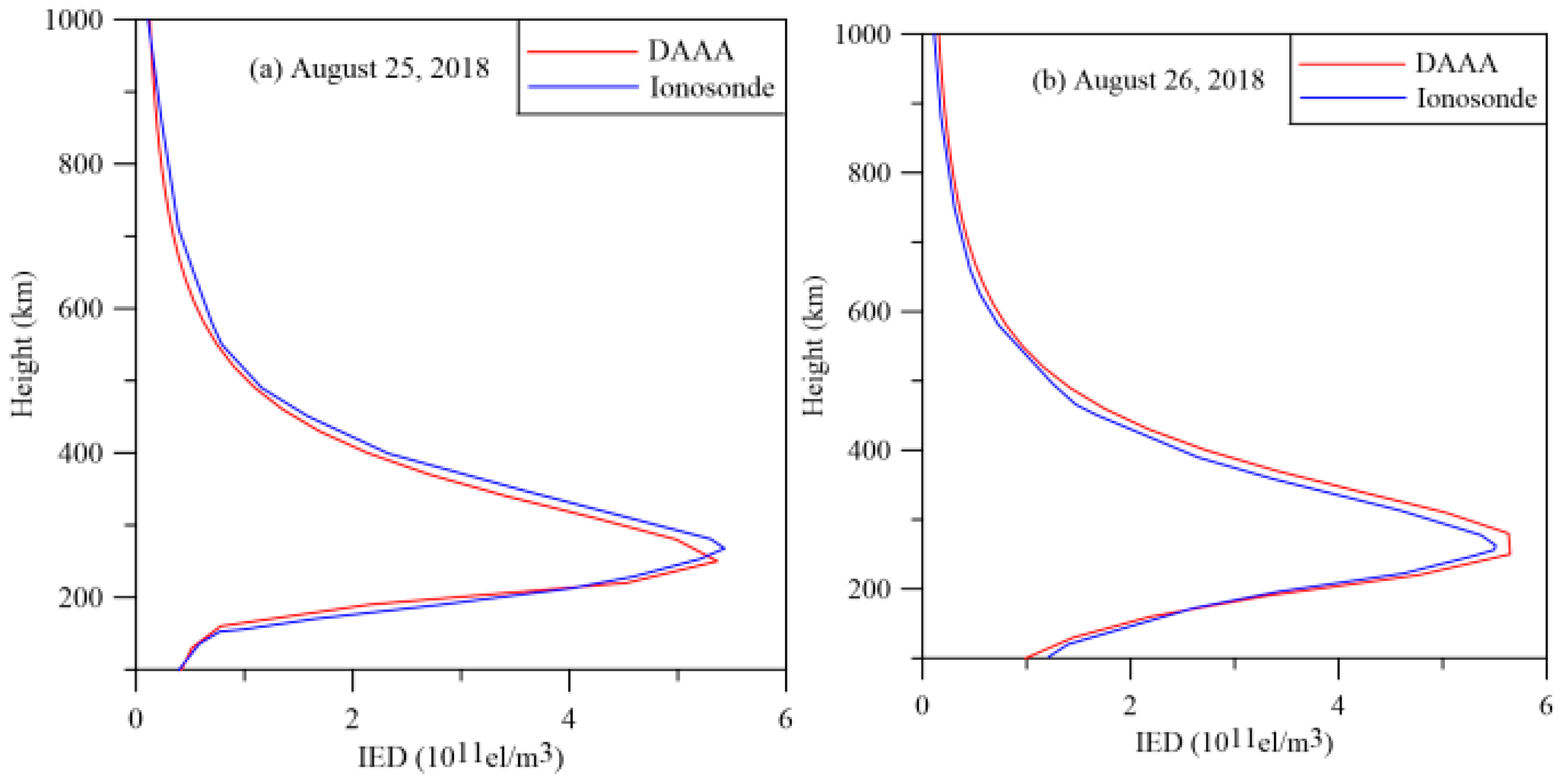
Figure 11 compares the reconstructed IED profiles with those obtained from the ionosonde data at Wuhan station in quiet geomagnetic and disturbed geomagnetic states. The comparisons of the ionospheric vertical profiles show that the reconstructed profiles of the DAAA method are in agreement with those obtained from ionosonde observation. The comparison validates the reliability and the practicality of the new algorithm during geomagnetic storms.

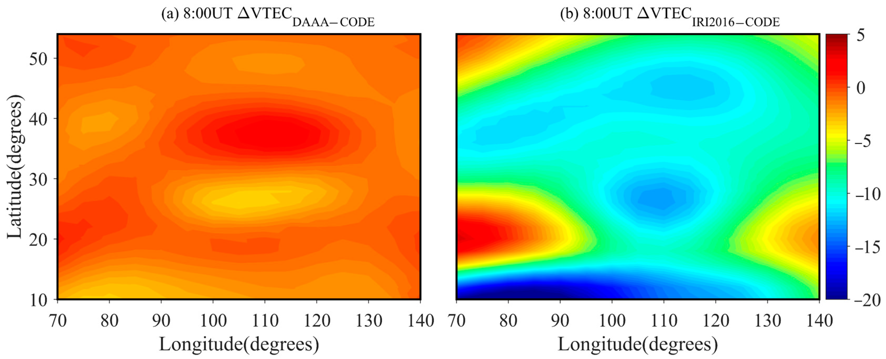
The VTEC can be obtained using the IED values inverted by the DAAA method and the IRI 2016 model during geomagnetic storm. The differential VTEC images are shown in Figure 12. Figure 12a shows that the maximum absolute of the differential VTEC is less than 4.5TECU. However, Figure 12b shows that the maximum absolute value of differential VTEC amounts to 20TECU. Figure 10 and Figure 12 validate that the DAAA method can effectively reflect the ionospheric change during geomagnetic storm.

5. Conclusions

This study develops a double-adaptive adjustment algorithm to reconstruct three-dimensional IED distributions by using the GNSS observation of CMONOC. Numerical simulation schemes are devised to verify the reliability and superiority of the DAAA algorithm. The test experiments confirm that the accuracy and the efficiency of the IED reconstruction can be improved by using the DAAA method. The diurnal variation is first studied on 3 September 2018. The reconstructed results of the DAAA method can accurately capture the formation, development and extinction of the equatorial anomaly core. Finally, a strong geomagnetic storm is selected as an analysis case. Comparing DAAA results with the reconstructed results in a quiet geomagnetic state, the positive and negative storm phase effect is found during the geomagnetic storm. Meanwhile, the IED slices and vertical profiles are compared. The comparisons show that the IRI 2016 model cannot reflect the true variations of the ionosphere under the condition of geomagnetic disturbance.

Although the DAAA can effectively reconstruct the three-dimensional IED distributions under different geomagnetic activities, the DAAA method has difficulty reconstructing the polar cap absorption event. In the future, the DAAA method will be extended to reconstruct solar flare and traveling ionospheric disturbances. In addition, the study of ionospheric activities caused by geohazards can be carried out using the DAAA.