Article

Improving the Detection Accuracy of Underwater Obstacles Based on a Novel Combined Method of Support Vector Regression and Gravity Gradient

1
School of Geomatics, Liaoning Technical University, Fuxin 123000, China
2
China Academy of Aerospace Science and Innovation, Beijing 100176, China
3
Qian Xuesen Laboratory of Space Technology, China Academy of Space Technology, Beijing 100094, China
*
Author to whom correspondence should be addressed.
These authors contributed equally to this work.
Remote Sens. 2023, 15(8), 2188; https://doi.org/10.3390/rs15082188
Submission received: 15 March 2023 / Revised: 12 April 2023 / Accepted: 17 April 2023 / Published: 20 April 2023
(This article belongs to the Special Issue Remote Sensing in Space Geodesy and Cartography Methods II)

Abstract

:
Underwater gravity gradient detection techniques are conducive to ensuring the safety of submersible sailing. In order to improve the accuracy of underwater obstacle detection based on gravity gradient detection technology, this paper studies the gravity gradient underwater obstacle detection method based on the combined support vector regression (SVR) algorithm. First, the gravity gradient difference ratio (GGDR) equation, which is only related to the obstacle’s position, is obtained based on the gravity gradient equation by using the difference and ratio methods. Aiming at solving the shortcomings of the GGDR equation based on Newton–Raphson method (NRM), combined with SVR algorithm, a novel SVR–gravity gradient joint method (SGJM) is proposed. Second, the differential ratio dataset is constructed by simulating the gravity gradient data generated by obstacles, and the obstacle location model is trained using SVR. Four measuring lines were selected to verify the SVR-based positioning model. The verification results show that the mean absolute error of the new method in the x, y, and z directions is less than 5.39 m, the root-mean-square error is less than 7.58 m, and the relative error is less than 4% at a distance of less than 500 m. These evaluation metrics validate the reliability of the novel SGJM-based detection of underwater obstacles. Third, comparative experiments based on the novel SGJM and traditional NRM were carried out. The experimental results show that the positioning accuracy of x and z directions in the obstacle’s position calculation based on the novel SGJM is improved by 88% and 85%, respectively.

1. Introduction

Underwater submersibles have been widely used in defense and scientific fields, such as underwater operations, marine research and mineral exploration, due to their ability to be concealed and high mobility [1,2]. For the smooth implementation of military and civilian technology, it is very necessary to ensure the safety of the underwater navigation of submersibles [3]. However, since the beginning of the 20th century, there have been nearly 500 accidents involving submersibles, of which about 20% were collision–sinking accidents, and these caused 84 submersibles to sink to the bottom of the sea [4]. Due to the complexity of the seabed environment, the imperfection of existing detection methods is one of the important reasons for the occurrence of many underwater accidents. In order to maintain concealment, submarines usually do not use active detection methods such as active sonar. As a result, it is difficult for the submarine to discover unexpected obstacles, causing collision accidents. Therefore, developing real-time, accurate, and passive underwater obstacle detection technology is crucial to ensure the safety of the underwater navigation of submersibles [5].
Underwater obstacle detection is an important part of underwater safety navigation; underwater obstacle detection technology uses acoustic signals, optical signals, electromagnetic signals, and gravity gradient signals for underwater obstacle detection [6]. The acoustic signal method mainly records the propagation time and phase difference of acoustic signals through sonar detection to estimate the azimuth and distance of underwater obstacles, which has the advantages of a large working range and is not affected by water turbidity. However, the acoustic signal method actively emits signals outward, resulting in the exposure of the submersible’s own position, which limits the practical application of the acoustic signal method [7]. The optical signal method obtains environmental information by receiving light from the surrounding environment with a high resolution and refresh rate. However, underwater light conditions (such as light absorption and scattering) are complex, and the detection range of optical signal methods is limited [8]. The electromagnetic sensor method can be applied in the underwater environment to achieve the estimation of underwater distance [9]. However, ambient electromagnetic fields can interfere with measurement accuracy [10]. The abovementioned underwater obstacle detection technologies have their own advantages and disadvantages, and researchers need to combine a variety of underwater detection technologies to complete various underwater obstacle detection tasks in practice. Based on this, as a passive detection method, the gravity gradient signal method has the characteristics of high sensitivity, can be concealed and can used in all weather types and in real time, which meets the requirements of the safe navigation of submersibles under concealed conditions and has an important application value [11,12,13].
Gravitational gradients reflect subtle changes in the gravitational field, and for high-density objects, accurate mass estimates can be made by measuring the gravitational gradient they cause [14]. Wu et al. [15,16,17] proposed an automatic full-tensor gravity gradient algorithm to estimate the mass, direction, and distance of underwater obstacles. Cheng et al. [18] combined gravity and gravity gradient information to detect the position and density of obstacles and concluded that the relative error of obstacle detection is within 5% under the condition that the accuracy of the gravimeter is 10−2 mGal and the accuracy of the gravimeter is 10−4 E. Wu and Cheng proposed that the method is feasible if the gravity gradient reference map in the detection area is known. Aiming at the obstacle detection problem in unknown sea areas (such as missing gravity gradient reference map or insufficient resolution). Yan et al. [19,20] proposed a gravity gradient difference ratio method without a gravity gradient reference map, which established a gravity gradient difference ratio (GGDR) equation only related to the obstacle’s position and used the Newton–Raphson method (NRM) to solve GGDR equation to obtain the obstacle’s position. However, if the initial value selected is not suitable when one is using NRM to solve the GGDR equation, the calculation result will not converge, and the detection accuracy will not be high. Nowadays, many articles focus on developing new submersibles and applying the regression surrogate model to solve some submersible problems. Chen et al. [21,22] were the first to apply machine learning algorithm to submersible fluid mechanics calculation and proposed the integration of multiple surrogate models, which improved the robustness of the model.
Different from previous research, this paper combines the characteristics of the gravity gradient difference ratio method and the characteristics of the SVR algorithm to propose a novel SVR–gravity gradient joint method (SGJM). The novel SGJM uses the gravity gradient difference ratio method to convert the obstacle detection problem into a higher order nonlinear equation solving problem, and then solves the higher order nonlinear equation using an SVR algorithm to determine the location of underwater obstacles. Firstly, the gravity gradient differential ratio data generated by simulated obstacles are calculated by the gravity gradient difference ratio method, and the differential ratio dataset is constructed by using the gravity gradient difference ratio data and the corresponding obstacle locations as the input and output, respectively. Then, based on the differential ratio dataset, the SVR obstacle localization model is trained, tested, and verified for reliability. Finally, the underwater obstacle’s positioning results of SGJM and NRM are compared in the same experimental environment, which verifies the improvement of obstacle’s positioning accuracy of SGJM in this paper. The novel SGJM ingeniously combines the gravity gradient with machine learning, which simplifies the conditions required for obstacle detection and improves the detection accuracy, and thus, it is a simple and practical method.

2. Methods

Earth is an irregularly shaped ellipsoid with uneven density distribution of its surface areas, resulting in differences in gravitational gradients throughout [23]. For example, the gravitational vertical gradient can be divided into two main parts: one part is the normal gravitational vertical gradient, assuming that it is caused by a rotating ellipsoid with uniform density distribution; the other part is the gravitational vertical gradient anomaly, which is caused by the difference between the gravitational vertical gradient and the normal gravitational vertical gradient caused by Earth. Similarly, the density of underwater obstacles and the surrounding environment will cause differences in gravity gradients, which include information such as the location and mass of underwater obstacles [24]. Therefore, under the condition that the accuracy of the gravity gradiometer is high enough, it is feasible to detect underwater obstacles by analyzing the gravity gradient caused by underwater obstacles.

2.1. Gravity Gradient Difference Ratio Method

The gravity gradient difference ratio method transforms obstacle detection problems into higher order nonlinear equation solving problems [20]. Suppose there is an obstacle with a uniform density distribution and a submersible carrying a gravity gradiometer in a seawater environment. The Cartesian coordinate system (right-handed system) is used to establish the obstacle at the origin of the center, and the x-axis is parallel to the submersible motion route and takes the submersible motion direction as the positive direction. Then, the center of mass coordinate of the obstacle in the Cartesian coordinate system is O 0 , 0 , 0 , and the coordinate of the submersible position is P x , y , z (the coordinates of the gravity gradiometer measurement are relative to the obstruction material center, reflecting the position of the obstacle). The t time gravitational gradient recorded by the submersible at point P can be described as [24]:
T o ( t ) T o x x ( t ) T o y y ( t ) T o z z ( t ) T o x y ( t ) T o x z ( t ) T o y z ( t ) + T n x x ( t ) T n y y ( t ) T n z z ( t ) T n x y ( t ) T n x z ( t ) T n y z ( t ) = G m r t 5 ( 3 x t 2 r t 2 ) G m r t 5 ( 3 y t 2 r t 2 ) G m r t 5 ( 3 z t 2 r t 2 ) 3 G m r t 5 x t y t 3 G m r t 5 x t z t 3 G m r t 5 y t z t + T n
where T o is the gravity gradient caused by the obstacle, T o D t is the component of the gravity gradient caused by the obstacle in the D = x x , y y , z z , x y , x z , y z direction, T n is the underwater environmental noise, T n D t is the value of underwater environmental noise in the D = x x , y y , z z , x y , x z , y z direction, G is the universal gravitational constant, m is the mass of the obstacle, x t , y t , z t is the coordinates at point P of the submersible position at the time of the t time measurement, and r t = x t 2 + y t 2 + z t 2 is the distance from the submersible position P point to the O point of the obstacle’s center at the t time measurement.
If two gravity gradient data are recorded in a short period of time during underwater navigation of the submersible, it can be considered that the difference between the two gravity gradient data is mainly caused by the relative change in position that occurs between the submersible and the underwater obstacle [24]. Therefore, the difference between the two adjacent gravity gradient data can eliminate underwater environmental noise T n , thereby isolating the submersible and obstacles from the surrounding environment. The gravity gradient difference Δ T is calculated as follows:
Δ T t = T o t + 1 T o t = Δ T x x t Δ T y y t Δ T z z t Δ T x y t Δ T x z t Δ T y z t = G m r t + 1 5 ( 3 x t + 1 2 r t + 1 2 ) G m r 5 ( 3 x t 2 r t 2 ) G m r t + 1 5 ( 3 y t + 1 2 r t + 1 2 ) G m r 5 ( 3 y t 2 r t 2 ) G m r t + 1 5 ( 3 z t + 1 2 r t + 1 2 ) G m r 5 ( 3 z t 2 r t 2 ) 3 G m r t + 1 5 x t + 1 y t + 1 3 G m r t 5 x t y t 3 G m r t + 1 5 x t + 1 z t + 1 3 G m r t 5 x t z t 3 G m r t + 1 5 y t + 1 z t + 1 3 G m r t 5 y t z t
where Δ T D t D = x x , y y , z z , x y , x z , y z is the component of the gravity gradient difference in the D direction.
From Equation (2), the gravity gradient difference Δ T still contains the mass of the obstacle after eliminating the ambient noise. Because the quality of the obstacle cannot be determined in advance, the influence of the quality of the obstacle can be eliminated by ratio, and the two gravity gradient difference data are divided to obtain the gravity gradient difference ratio function [20], which is only related to the position of the obstacle:
r Δ T ( t ) = Δ T ( t ) / Δ T ( t + 1 ) = T o t + 1 T o t / T o t + 2 T o t + 1 = r Δ T x x ( t ) r Δ T y y ( t ) r Δ T z z ( t ) r Δ T x y ( t ) r Δ T x z ( t ) r Δ T y z ( t ) = r t + 1 5 ( 3 x t + 1 2 r t + 1 2 ) r t 5 ( 3 x t 2 r t 2 ) r t + 2 5 ( 3 x t + 2 2 r t + 2 2 ) r t + 1 5 ( 3 x t + 1 2 r t + 1 2 ) r t + 1 5 ( 3 y t + 1 2 r t + 1 2 ) r t 5 ( 3 y t 2 r t 2 ) r t + 2 5 ( 3 y t + 2 2 r t + 2 2 ) r t + 1 5 ( 3 y t + 1 2 r t + 1 2 ) r t + 1 5 ( 3 z t + 1 2 r t + 1 2 ) r t 5 ( 3 z t 2 r t 2 ) r t + 2 5 ( 3 z t + 2 2 r t + 2 2 ) r t + 1 5 ( 3 z t + 1 2 r t + 1 2 ) r t + 1 5 x t + 1 y t + 1 r t 5 x t y t r t + 2 5 x t + 2 y t + 2 r t + 1 5 x t + 1 y t + 1 r t + 1 5 x t + 1 z t + 1 r t 5 x t z t r t + 2 5 x t + 2 z t + 2 r t + 1 5 x t + 1 z t + 1 r t + 1 5 y t + 1 z t + 1 r t 5 y t z t r t + 2 5 y t + 2 z t + 2 r t + 1 5 y t + 1 z t + 1
where r Δ T is gravity gradient difference ratio, and r Δ T D t D = x x , y y , z z , x y , x z , y z is the component of the gravity gradient difference ratio in the D direction.
Equation (3) is further expanded into the integral form, and the gravity gradient difference ratio integral function, which is only related to the position of the obstacle, is obtained:
r Δ T x x ( t ) r Δ T y y ( t ) r Δ T z z ( t ) r Δ T x y ( t ) r Δ T x z ( t ) r Δ T y z ( t ) = r t + 1 5 3 x t + 1 a 2 r t + 1 2 r t 5 3 x t a 2 r t 2 r t + 2 5 3 x t + 2 a 2 r t + 2 2 r t + 1 5 3 x t + 1 a 2 r t + 1 2 d a d b d c r t + 1 5 3 y t + 1 b 2 r t + 1 2 r t 5 3 y t b 2 r t 2 r t + 2 5 3 y t + 2 b 2 r t + 2 2 r t + 1 5 3 y t + 1 b 2 r t + 1 2 d a d b d c r t + 1 5 3 z t + 1 c 2 r t + 1 2 r t 5 3 z t c 2 r t 2 r t + 2 5 3 z t + 2 c 2 r t + 2 2 r t + 1 5 3 z t + 1 c 2 r t + 1 2 d a d b d c r t + 1 5 x t + 1 a y t + 1 b r t 5 x t a y t b r t + 2 5 x t + 2 a y t + 2 b r t + 1 5 x t + 1 a y t + 1 b d a d b d c r t + 1 5 x t + 1 a z t + 1 c r t 5 x t a z t c r t + 2 5 x t + 2 a z t + 2 c r t + 1 5 x t + 1 a z t + 1 c d a d b d c r t + 1 5 y t + 1 b z t + 1 c r t 5 y t b z t c r t + 2 5 y t + 2 b z t + 2 c r t + 1 5 y t + 1 b z t + 1 c d a d b d c
where the integral area of the integral function is the space surrounded by the outline of the obstacle; a , b , c is the product element coordinate of the obstacle object; r t = x t a 2 + y t b 2 + z t c 2 ; if Δ s is the gravity gradient recording distance interval, then x t + 1 = x t + Δ s , y t = y t + 1 , and z t = z t + 1 .
Equation (4) is converted to the following:
r Δ T x x ( t ) r Δ T y y ( t ) r Δ T z z ( t ) r Δ T x y ( t ) r Δ T x z ( t ) r Δ T y z ( t ) r t + 1 5 3 x t + 1 a 2 r t + 1 2 r t 5 3 x t a 2 r t 2 r t + 2 5 3 x t + 2 a 2 r t + 2 2 r t + 1 5 3 x t + 1 a 2 r t + 1 2 d a d b d c r t + 1 5 3 y t + 1 b 2 r t + 1 2 r t 5 3 y t b 2 r t 2 r t + 2 5 3 y t + 2 b 2 r t + 2 2 r t + 1 5 3 y t + 1 b 2 r t + 1 2 d a d b d c r t + 1 5 3 z t + 1 c 2 r t + 1 2 r t 5 3 z t c 2 r t 2 r t + 2 5 3 z t + 2 c 2 r t + 2 2 r t + 1 5 3 z t + 1 c 2 r t + 1 2 d a d b d c r t + 1 5 x t + 1 a y t + 1 b r t 5 x t a y t b r t + 2 5 x t + 2 a y t + 2 b r t + 1 5 x t + 1 a y t + 1 b d a d b d c r t + 1 5 x t + 1 a z t + 1 c r t 5 x t a z t c r t + 2 5 x t + 2 a z t + 2 c r t + 1 5 x t + 1 a z t + 1 c d a d b d c r t + 1 5 y t + 1 b z t + 1 c r t 5 y t b z t c r t + 2 5 y t + 2 b z t + 2 c r t + 1 5 y t + 1 b z t + 1 c d a d b d c = 0
Equation (5) is a high-order nonlinear equation. Traditional NRM is generally used to solve higher order nonlinear equations. However, as NRM is an iterative algorithm, the selection of initial values is very important, and inappropriate initial values will lead to nonconvergence of the calculation results and a low detection accuracy. Therefore, in order to improve the accuracy of obstacle detection, the SVR algorithm is used to solve the GGDR equation.

2.2. Support Vector Regression

The SVR algorithm is a machine learning algorithm that was proposed by Vapnik et al. [25] in the 1990s, which is used to solve regression problems. The SVR algorithm takes structural risk minimization as the basic idea of machine learning, and compared with the traditional statistical theory, this algorithm specializes in the statistical law of machine learning in the case of small samples [26]. In addition, the SVR algorithm is able to approximate the solution of higher order nonlinear equations. Thus, SVR was chosen as a surrogate model in this study [27]. As shown in Figure 1, the idea of the SVR algorithm is to find a hyperplane so that as many points as possible are concentrated in a space that is as small as possible on both sides of the hyperplane.
Given a dataset A = m i i n (where m i represents the 6-dimensional input vector, i = 1 , 2 , n , n is the length of the dataset), the nonlinear kernel function is mapped to the high-dimensional feature space to complete linear regression. In the high-dimensional feature space, the SVR algorithm uses the following approximation function [28]:
h = f m = ω ϕ m + l
where ϕ m represents the high-dimensional feature space of the input vector, m , for nonlinear mapping. The weight factor ω and constant l are solved with the optimization model of the optimal regression function [28]:
Minimize : 1 2 ω 2 + C i = 1 n ( ξ i + ξ i ) , C > 0 Subject to : h i ω ϕ m i + l i ε + ξ i ω ϕ m i + l i h i ε + ξ i * ξ i , ξ i * 0
where C is the penalty factor for balancing empirical risk and model flatness, ξ i and ξ i * are relaxation variables that constrain the output of the system, and ε is the tube size constant [29].
Equation (7) is a convex optimization problem, which can be solved by the Lagrange multiplier method. The Lagrange multiplier is introduced, and the regression function of SVR algorithm is calculated as follows [30]:
f m = i = 1 n λ i , λ i * K m , m i + l
where λ i and λ i * are Lagrange multipliers, λ i 0 , λ i * 0 , i = 1 , 2 , n . K ( m , m i ) is a kernel function, K ( m , m i ) = ϕ ( m ) T × ϕ ( m i ) .
Kernel functions help researchers to deal with feature spaces of any dimension without explicitly calculating mapping, ϕ m . Any function that satisfies the Mercer condition can be used as a kernel function [31]. Table 1 describes the categories and expressions of several commonly used kernel functions [32]:
The kernel parameters are manually set, and when the parameters are determined, it means that the kernel function is determined. The parameter selection of the kernel function directly affects the prediction accuracy of SVR [33]. The selection of kernel parameters should be cautiously performed because it implicitly defines the structure of high-dimensional feature space, thus controlling the complexity of the final solution [34]. In this paper, RBF is used as the kernel function of the SVR algorithm.
As a machine learning algorithm, the SVR algorithm is a supervised learning algorithm that regresses the target samples according to the current sample information. SVR implicitly expresses the mathematical relationship between the input vector and output value.

2.3. SVR–Gravity Gradient Joint Method

From the analysis in Section 2.1, the mathematical relationship between the gravity gradient difference ratio and the position of the obstacle is established by the GGDR equation, and the obstacle detection problem is transformed into the problem of solving higher order nonlinear equations [20]. From the analysis in Section 2.2, it can be seen that the SVR algorithm simplifies the mathematical relationship between the gravity gradient difference ratio and the position of the obstacle to some extent [35], and it can better approach the solution of the equation for higher order nonlinear equations [27]. Therefore, this paper combines the characteristics of the gravity gradient difference ratio method and the SVR algorithm and proposes the novel SVR–gravity gradient joint method (SGJM).
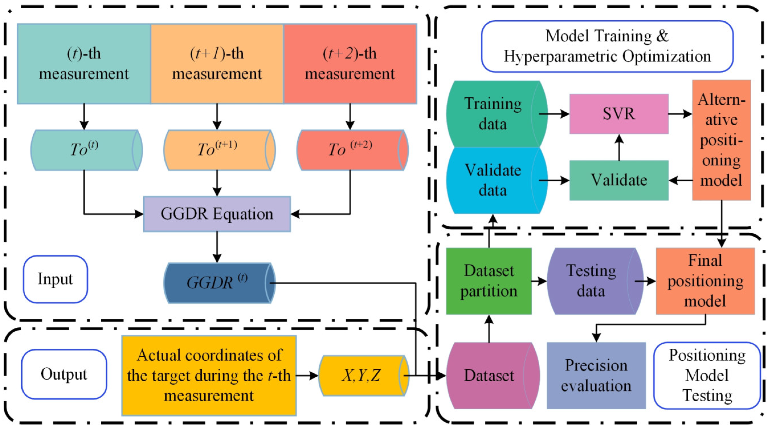
In the composition of SGJM, the simulated gravity gradient data are transformed into a gravity gradient difference ratio by Equation (3). Then, the gravity gradient difference ratio and the position of obstacles are used as the input and output of the SVR algorithm, respectively, to construct the difference ratio dataset, and the SVR obstacle location model is obtained by training. Finally, the location model is used to solve the GGDR equation and evaluate the positioning accuracy. As shown in Figure 2, the novel SGJM consists of three parts: data simulation, positioning model training, and accuracy evaluation.
In SVR obstacle location model training, this paper uses the grid search method [36] and the 5-fold cross-validation method [37] to optimize the SVR regression model, and the super parameters are penalty parameter, C , kernel function coefficient, γ , and tube size, ε .
The result of obstacle location is compared with the real position of the obstacle, and the reliability of underwater obstacle location based on SGJM is evaluated by mean absolute error (MAE), root-mean-square error (RMSE), coefficient of determination (R2), relative error (RE), and signal-to-noise ratio (SNR). The smaller the MAE and RMSE are, the closer the result is to the real value. The closer R2 is to 1, the higher the fitting degree of the SVR regression model is. The relative error reflects the credibility of the measurement, and the smaller the RE is, the higher the credibility is. The signal-to-noise ratio reflects the influence of noise in the signal, and the larger the SNR is, the smaller the noise is. The corresponding definition is [38,39,40,41]:
M A E = 1 n i = 1 k g i h i
R M S E = 1 n i = 1 k ( g i h i ) 2
R 2 = 1 S S E S S T
R E = g i h i g i
S N R = log 10 S / N
where g i is the true value of the obstacle coordinates, h i is the calculated value of the obstacle coordinates, i = 1 , 2 , k , k is the length of the test set, S S E is the square sum of the residuals, S S T is the total square sum, S is the gravity gradient signal power, and N is the noise power.

3. Novel SGJM Verification

The reliability of the novel SGJM is verified by simulation experiment. First, the gravity gradient anomaly caused by obstacles is simulated and converted into the gravity gradient difference ratio to construct the difference ratio dataset for the training of the SVR algorithm. Second, the SVR obstacle location model is trained. Finally, four measuring lines are designed, and the gravity gradient data on the simulated lines are input into the SVR positioning model to verify the positioning reliability of SGJM.

3.1. Data Simulation

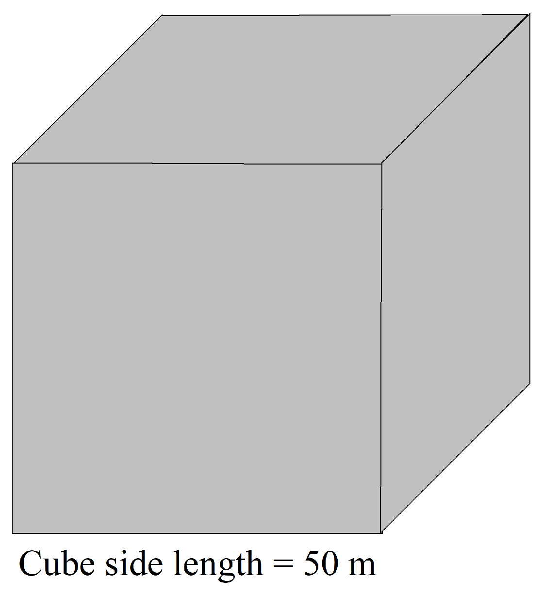
Using protruding rocks on the seabed as reference objects to construct simulated obstacles, a size equivalent to the length of a large submersible and regular-shaped obstacles are selected for the ease of calculation. The simulated obstacle is constructed. The simulated obstacle is a solid cube prism with 50 m × 50 m × 50 m, and the density distribution is uniform and set to σ = 2.7 t/m3, as shown in Figure 3. (This article does not consider the impact of errors caused by uniform density, which will be discussed in the team’s subsequent research.) The gravity gradient data simulation area range is 1000 m × 1000 m × 200 m, the centroid of the model is located in the vertical projection center of the data simulation area, and the data simulation point parameters are shown in Table 2. Each point can separately generate a set of gravity gradient difference ratio data according to Equation (4). Here, the sensitivity of the gravity gradiometer is assumed to be 10−5 E. Therefore, environmental noise with a root-mean-square error of 10−5 E is added to the initial simulated gravity gradient data to verify the reliability of the novel SGJM. Simulated data with noise are used to train and verify the regression model.
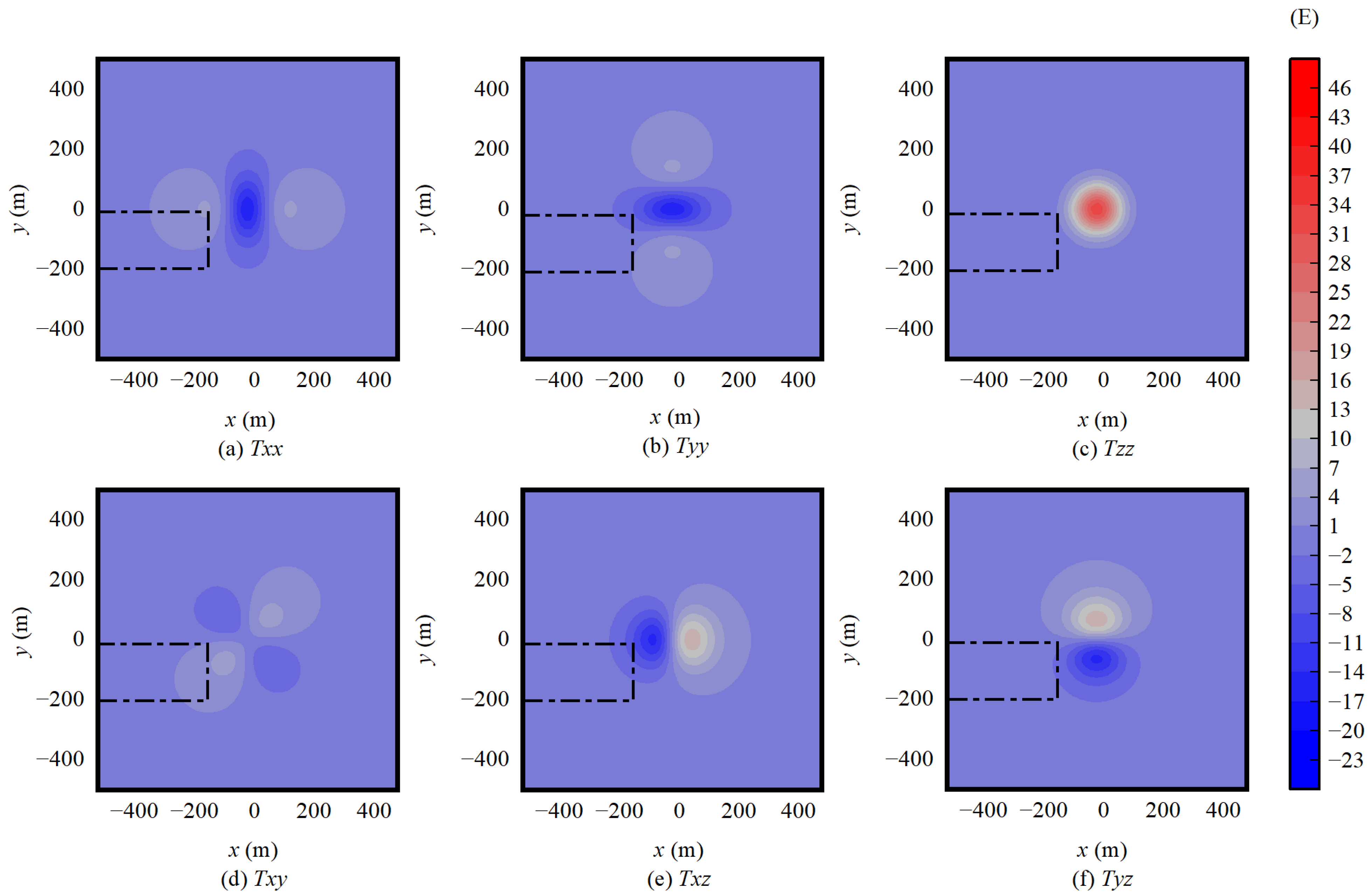
Combined with Equation (1), the gravity gradient distribution caused by the simulated obstacle (cube prism) in the z = 100 m plane is obtained, as shown in Figure 4. The gravity gradient caused by the simulated obstacle at the level of 100 m above it shows a very regular distribution and different trends for different gravity gradient components. The maximum value of gravity gradient anomaly is 44.5 E, the minimum value is −22.3 E, the mean value is −6 × 10⁻⁸ E, and the resolution is 10 m × 10 m. When the submersible vehicle sails along the direction parallel to the x-axis toward the obstacle, the coordinate of the submersible vehicle is always negative relative to the x direction of the obstacle. Therefore, it is only necessary to establish the relationship between the gravity gradient characteristics of the obstacle in the negative direction of the x-axis and the position of the obstacle. Assuming that the obstacle is located on the left side of the forward direction of the submersible, the gravity gradient difference ratio data generated by the points in Table 2, in the range of x 500 , 130 , y 200 , 10 , and z 10 , 200 , are selected as the data of the reliability verification experiment. As shown in Figure 4, the area surrounded by the dotted line is the selected area in the experiment.
In order to understand the relationship more intuitively between the detection accuracy and the detection distance of the gravity gradiometer, the relationship between the gravity vertical gradient accuracy and the detection distance is obtained by calculating and simulating the gravity vertical gradient produced by the obstacle on different straight line distances, as shown in Figure 5. According to Figure 5b, the underwater obstacle detection method based on gravity gradient can detect underwater obstacles within a straight line distance of 700 m when the accuracy of the gravity gradiometer is 10−2 E, underwater obstacles within a straight line distance of 1200 m when the accuracy of the gravity gradiometer is 10−3 E, and underwater obstacles within a straight line distance of 1700 m when the accuracy of the gravity gradiometer is 10−4 E. Therefore, the gravity gradient data caused by simulated obstacles with the accuracy of 10−5 E meet the accuracy requirements of underwater obstacle detection method based on gravity gradient to detect obstacles within a straight line distance of 700 m.
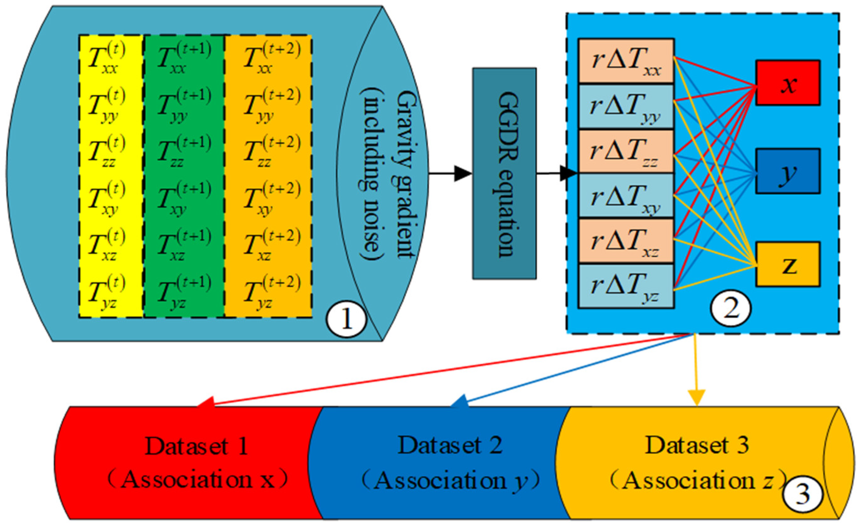
The simulated gravity gradient data are transformed into the gravity gradient difference ratio with Equation (3). The gravity gradient difference ratio is used as the input, and the corresponding obstacle’s position is used as the output to construct the difference ratio dataset to prepare for SVR obstacle location model training in the following step. The sample size of the difference ratio dataset is 15,200, and each sample contains six features (the component of the gravity gradient in the D = x x , y y , z z , x y , x z , y z direction) and three expected values x , y , z . The construction method of differential ratio dataset for positioning model training is shown in Figure 6. In the first step, the full tensor gravity gradient anomaly caused by obstacles is calculated and simulated by Equation (1), and the environmental noise with root-mean-square error of 10−5 E is added. The second step is to calculate the gravity gradient difference ratio, r Δ T , input the gravity gradient data into Equation (3), and output the gravity gradient difference ratio, which correspond to the calculated point coordinates. In the third step, the difference ratio dataset is divided into three datasets according to different coordinate components, and r Δ T is combined with x , y , and z , respectively, to obtain dataset 1 (for training the model positioned in the x direction), dataset 2 (for training the model positioned in the y direction), and dataset 3 (for training the model positioned in the z direction).

3.2. Verification of SVR Positioning Model

The reliability of underwater obstacle detection based on the novel SGJM is verified by simulation experiments. Four lines are designed according to whether the underwater obstacle is on the forward path or not, and the gravity gradient difference ratio generated on the four lines is used as the input vector. The obstacle location was obtained by the SVR positioning model (containing three positioning models in the x direction, y direction, and z direction), and then the reliability of the novel SGJM was verified by comparing the true value of the obstacle’s location and the calculated value.

3.2.1. Data Preprocessing

In the process of data simulation, the gravity gradient value spans several orders of magnitude, and the quotient of the difference between large order and small order gravity gradients will lead to outliers in the calculation results of gravity gradient difference ratio. Outliers will have a negative impact on the regression results of the SVR positioning model [42]. In order to produce a better training model, it is necessary to control the data in a stable interval. First of all, the gravity gradient difference ratio data are analyzed, and the initial threshold is selected to eliminate the large outliers for the first time; then, the absolute median deviation algorithm (MAD) is used to determine the outliers by judging whether the deviation of each element and the median is within a reasonable range, and then eliminate the outliers. The specific calculation formula of the median deviation algorithm is as follows [43]:
M A D = median r Δ T i median r Δ T
where median Ψ is the median of all the elements in Ψ .
The data are adjusted through M A D as follows:
r Δ T i = r Δ T i , median r Δ T ν M A D r Δ T i median r Δ T + ν M A D , others
where ν is the parameter, the value of which in this paper is three. This value is an empirical value, which means a median deviation of three times [44].
The differential ratio dataset is divided into a training set, a verification set, and a test set. The training set is used to train the parameters in the SVR positioning model; the verification set is usually used to adjust the hyperparameters, which has the best performance according to the performance of several groups of models on the verification set; the test set is used to evaluate the generalization ability of the model. In this paper, the data of four lines in the differential ratio dataset are extracted as the test set, 80% of the data is randomly extracted as the training set, and the remaining 20% is used as the verification set.

3.2.2. Experimental Parameter Setting

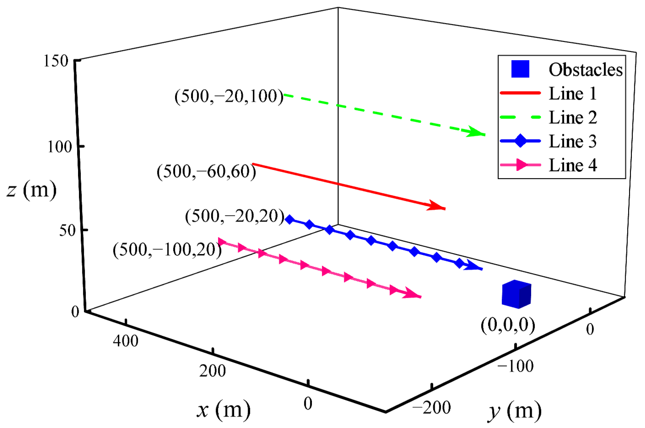
The submersible vehicle will collide or not collide underwater. In this paper, four measuring lines are designed, named as Line 1, Line 2, Line 3, and Line 4, and the obstacles are in the direction of Line 3. Assuming that there are no other high-density objects in the environment of the submersible vehicle and the obstacle, the submersible vehicle moves in the x direction at a speed of 10 m/s, and the built-in gravity gradiometer records data once a second. In Figure 7, the solid line is Line 1, and the initial position coordinates of the submersible are 500 , 60 , 60 ; the dotted line is Line 2, and the initial position coordinates of the submersible are 500 , 20 , 100 ; the rhomboid line is Line 3, and the initial position coordinates of the submersible are 500 , 20 , 20 ; the triangular line is Line 4, and the initial position coordinates of the submersible are 500 , 100 , 20 ; the cube is the obstacle.

3.2.3. Results and Analysis

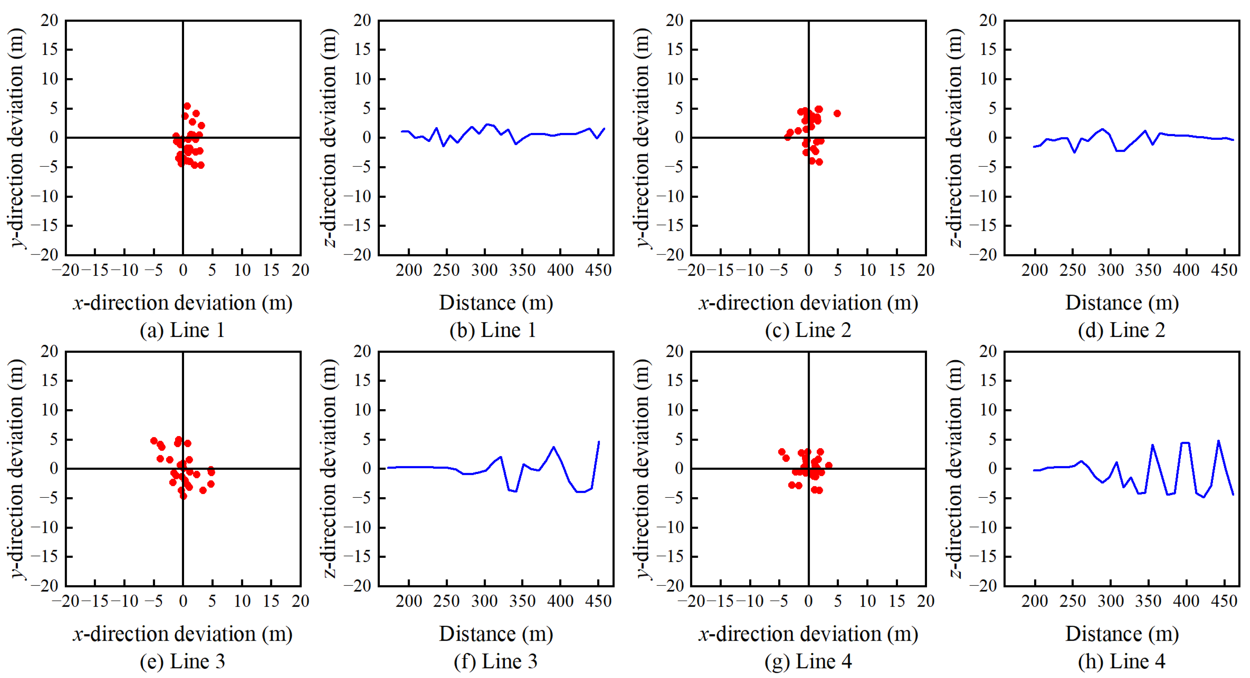
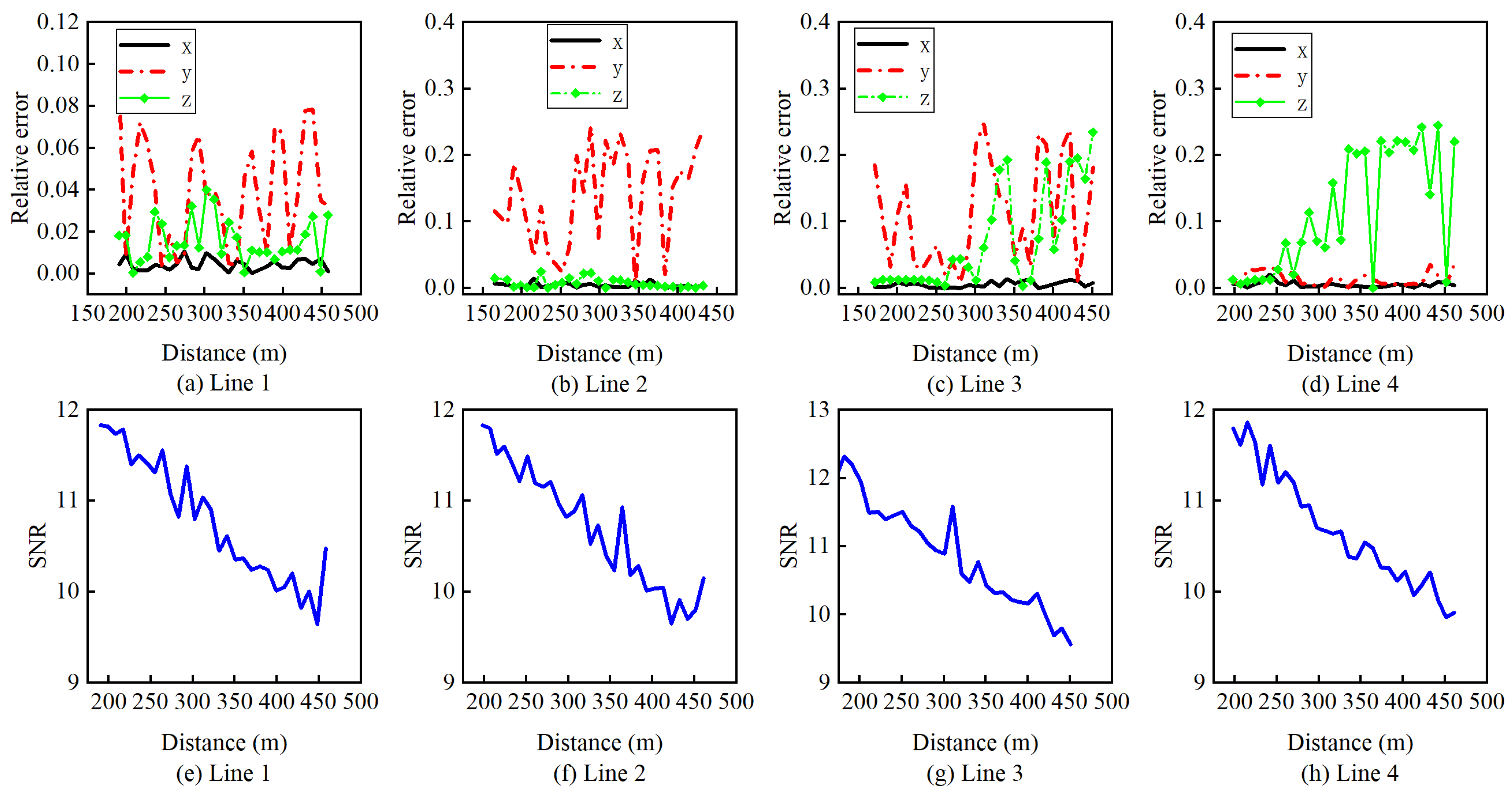
The gravity gradient difference ratio data of the four lines are input into the SVR obstacle location model in turn to obtain the calculation results of the obstacle’s position. The MEA and RMSE of the positioning error are obtained by counting the calculated value and true value of the obstacle’s position, as shown in Table 3. R2 of the x direction positioning model of the four lines is 0.993~0.999, which proves that the fitting degree of the positioning model is high. Because there is no change in the coordinates of the y direction and z direction in each line, it is impossible to calculate the coefficient of determination of the positioning model in the y direction and the z direction. The three direction positioning errors of each measuring line detecting obstacles are shown in Figure 8, and the SNR and RE are shown in Figure 9.
According to Table 3, the MEA of the underwater obstacle detection results of Lines 1~4 is about 2.25 m, and the MEA range is 0.71~5.39 m. Among them, the maximum value of MAE in x direction is 2.52 m, and the minimum value is 1.34 m; the maximum value of MAE in y direction is 5.39 m, and the minimum value is 1.43 m; the maximum value of MAE in z direction is 3.39 m, and the minimum value is 0.71 m. The RMSE of Lines 1~4 for underwater obstacle detection is about 3.48 m, and the range is 0.99~7.58 m. According to [45], the MAE of the traditional acoustic underwater positioning algorithm is 7.05 m. Therefore, the positioning accuracy of the novel SGJM is better than that of the traditional underwater positioning methods.
According to Figure 8, detection errors in the x, y, and z directions in Lines 1~4 are mostly −5~5 m. According to Figure 8a–d, the positioning effect of measuring Lines 1~2 is better in the x direction and the z direction; according to Figure 8g,h, the positioning effect of measuring Line 4 in the y direction is better; according to Figure 8e,f, the positioning result of measuring Line 3 is relatively poor compared with those of Lines 1, 2, and 4, but the positioning error is still within the size range of obstacles, and it can still locate obstacles accurately. Therefore, the positioning results of Figure 8 prove the effectiveness and reliability of the novel SGJM.
According to Figure 9a–d, the RE of underwater obstacle location errors in the x direction of Lines 1~4, the z direction of Lines 1~2, and the y direction of Line 4 are less than 4% when the distance is less than 500 m, and the RE of underwater obstacle location error in the y direction of Line 1 is less than 8% when the distance is less than 500 m. The RE in other directions is unstable, and the maximum RE is 24.6%. According to Figure 9e–h, with the increase in distance, the SNR decreases, and the influence of environmental noise increases. Table 4 shows the RE averages of the x, y, and z directions in Lines 1~4.
According to Table 4, there are differences in the positioning accuracy among different measuring lines, and the reason for the differences is the different positions of measuring lines. Because the position of Line 3 in the SVR obstacle location model is closer to the boundary of the differential ratio dataset used for training, the fitting effect is not as strong as that of Line 1, which is close to the simulated data center; the y direction of Line 2 and the z direction of Line 4 are also close to the boundary of the dataset, and the data imbalance leads to relatively poor positioning results in the corresponding direction. The reason for the large RE in some directions in Lines 2~4 is that the true values of y and z are small, which leads to the large RE. A large relative error does not necessarily mean poor positioning results in the y and z directions. According to MAE, the positioning results in the y and z directions are comparable to those in the x direction. The optimal application range of the novel SGJM is between 20 m and 500 m.

4. Application

The novel SGJM is applied to an underwater obstacle detection task, and the traditional NRM [20] is used as a comparison to prove that SGJM has better detection accuracy. The simulation experiment is established, and the underwater obstacle is a cuboid prism of 80 m × 40 m × 20 m with a density of 2.7 t/m3. Taking the center of the obstacle matter as the coordinate origin, the Cartesian coordinate system (right-handed system) is established. The motion direction of the submersible is parallel to the positive direction of the x-axis, the coordinates of the starting point are 400 , 70 , 60 , and the velocity is 10 m/s. The gravity gradiometer records data once a second. The environmental noise with RMSE of 10−5 E is added to the simulated gravity gradient data, and a total of 23 sets of gravity gradient differential ratio data are obtained.
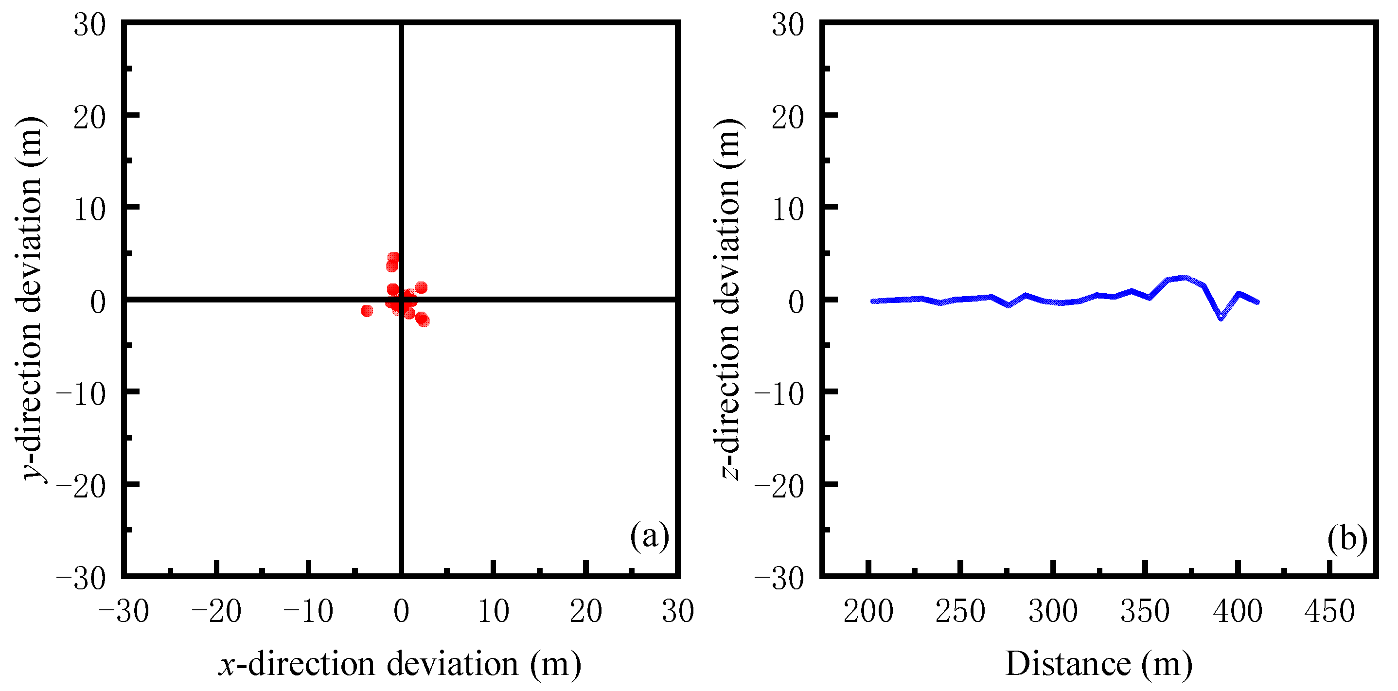
In this experiment, 23 simulated localizations were performed, and after statistical analysis, the MAE, RMSE, and standard deviation (STD) of the localization results were obtained, and the results are shown in Table 5. t-test was carried out based on the normal distribution, and the difference level of positioning error between SGJM and NRM was obtained, as shown in Table 6. The positioning error of the novel SGJM is shown in Figure 10. The positioning error of the traditional NRM is shown in Figure 11. The SNR of SGJM and NRM is shown in Figure 12a, and the RE comparison is shown in Figure 12b and Figure 13.
According to Table 5, both MAE and RMSE of SGJM are smaller than NRM is, the MAE and RMSE of SGJM in the y direction are slightly better than NRM is, and the MAE and RMSE of SGJM in the x direction and z direction are obviously better than those of NRM. Among them, the precision in the x direction has been improved by 88%, the precision in the y direction has been improved by 6%, and the precision in the z direction has been improved by 85%. The improvement of positioning accuracy in the y direction is lower because the positioning accuracy of NRM in the y direction is higher.
According to Table 6, the positioning accuracy of SGJM is better than that of NRM in x and z directions. There is no significant difference in the positioning results in the y direction.
According to Figure 10 and Figure 11, the positioning error of SGJM is obviously better than that of NRM. The positioning error of SGJM increases with the increase in distance, but it is still within the range of −4~4 m. According to Figure 12a, with the increase in distance, the SNR decreases, and the influence of environmental noise increases. According to Figure 12b and Figure 13, the RE of NRM is less than 6% when the distance is less than 360 m; the RE is less than 4% when the distance of SGJM is less than 410 m, and the RE is less than 2% when the distance is less than 290 m. The obstacle location accuracy of SGJM is higher than that of NRM.
In summary, the average MEA of the obstacle localization results obtained by the novel SGJM is only about 1/5 of that of NRM. The relative error of SGJM is less than 4%, which is better than 6% of NRM. Therefore, the novel SGJM effectively improves the positioning accuracy of the traditional NRM.

5. Conclusions

The detection of underwater obstacles based on the gravity gradient is studied in this paper. A novel combined SVR–gravity gradient method (SGJM) is proposed to locate the abnormal obstacles in the range of 150~450 m. The underwater navigation concealment and the safety of the underwater vehicle are ensured. The specific conclusions are as follows:
(1)
A novel SVR–gravity gradient joint method (SGJM) is constructed. Firstly, based on the gravity gradient calculation formula, the difference method and ratio method are used to eliminate the environmental and mass effects, and the gravity gradient difference ratio (GGDR) equation is obtained. In order to solve the problem of NRM being difficult to converge, thereby leading to low accuracy in obstacle location when solving high-order nonlinear equations, the SVR algorithm is introduced to solve GGDR equations. The SVR algorithm is a machine learning algorithm that can approach the solution of higher order nonlinear equations well. This paper combines the gravity gradient difference ratio method and the SVR algorithm, constructs the difference ratio dataset for machine learning training through the gravity gradient difference ratio method, and trains the SVR obstacle location model to be suitable for specific obstacles based on the SVR algorithm.
(2)
The reliable verification of obstacle location detection is based on the novel SGJM. Firstly, the gravity gradient data generated by a simulated obstacle (cube) with a size of 50 m × 50 m × 50 m, and uniform density distribution is calculated, and the difference ratio dataset for machine learning is constructed by the gravity gradient difference ratio function. Then, the SVR obstacle location model is trained based on the SVR algorithm. Finally, the positioning accuracy of the positioning model is tested with four measuring lines. The experimental results show that the MAE and RMSE of the positioning results are less than 5.39 m and 7.58 m in the x, y, and z directions, respectively, and the RE in x direction is less than 4% when the distance is less than 500 m.
(3)
The positioning results of the novel SGJM, compared with those of NRM, in the x, y, and z directions are 1.31 m, 0.92 m, and 1.14 m under the same experimental conditions, which are 88%, 6%, and 85% higher than those of NRM. The RMSE in the x, y, and z directions are 1.92 m, 1.54 m, and 1.69 m, and the RE is less than 4% within a 400 m distance.

Author Contributions

Conceptualization, T.F., W.Z. and Z.L.; methodology, T.F.; formal analysis, T.F. and W.Z.; investigation, T.F.; data curation, T.F.; writing—original draft preparation, T.F.; writing—review and editing, T.F., W.Z., Z.L., Y.S., H.Z. and A.X.; funding acquisition, W.Z. and A.X.; All authors have read and agreed to the published version of the manuscript.

Funding

This work was supported in part by the National Natural Science Foundation of China under Grant (42274119), in part by the Liaoning Revitalization Talents Program under Grant (XLYC2002082), in part by National Key Research and Development Plan Key Special Projects of Science and Technology Military Civil Integration (2022YFF1400500), and in part by the Key Project of Science and Technology Commission of the Central Military Commission.

Acknowledgments

We greatly appreciate the helpful suggestions from editors and anonymous reviewers.

Conflicts of Interest

The authors declare no conflict of interest.

References

  1. Angevine, R.G. Innovation and Experimentation in the US Navy: The UPTIDE Antisubmarine Warfare Experiments, 1969–1972. J. Strateg. Stud. 2005, 28, 77–105. [Google Scholar] [CrossRef]
  2. Ura, T. Observation of Deep Seafloor by Autonomous Underwater Vehicle. Indian J. Mar. Sci. 2013, 42, 1028–1033. [Google Scholar]
  3. Ganesan, V.; Chitre, M.; Brekke, E. Robust Underwater Obstacle Detection and Collision Avoidance. Auton. Robots 2016, 40, 1165–1185. [Google Scholar] [CrossRef]
  4. Cai, H. Research on Obstacle Avoidance for Submarines Based on Gravity Anomalies. Ship Electronic Engineering. Ship Electron. Eng. 2011, 31, 76–78. (In Chinese) [Google Scholar]
  5. HSDL—Design for Undersea Warfare, Update One: Commander’s Guidance for the United States Submarine Force and Supporting Undersea Forces. Available online: https://www.hsdl.org/c/abstract/?docid=726701 (accessed on 11 April 2023).
  6. Cong, Y.; Gu, C.; Zhang, T.; Gao, Y. Underwater Robot Sensing Technology: A Survey. Fundam. Res. 2021, 1, 337–345. [Google Scholar] [CrossRef]
  7. Tian, H.; Guo, S.; Zhao, P.; Gong, M.; Shen, C. Design and Implementation of a Real-Time Multi-Beam Sonar System Based on FPGA and DSP. Sensors 2021, 21, 1425. [Google Scholar] [CrossRef]
  8. Köser, K.; Frese, U. Challenges in Underwater Visual Navigation and SLAM. In AI Technology for Underwater Robots; Kirchner, F., Straube, S., Kühn, D., Hoyer, N., Eds.; Intelligent Systems, Control and Automation: Science and Engineering; Springer International Publishing: Cham, Switzerland, 2020; pp. 125–135. ISBN 978-3-030-30683-0. [Google Scholar]
  9. Kwak, K.; Park, D.; Chung, W.K.; Kim, J. Underwater 3-D Spatial Attenuation Characteristics of Electromagnetic Waves With Omnidirectional Antenna. IEEE ASME Trans. Mechatron. 2016, 21, 1409–1419. [Google Scholar] [CrossRef]
  10. Ji, C.; Chen, Q.; Song, C. Improved Particle Swarm Optimization Geomagnetic Matching Algorithm Based on Simulated Annealing. IEEE Access 2020, 8, 226064–226073. [Google Scholar] [CrossRef]
  11. Sheinker, A.; Ginzburg, B.; Salomonski, N.; Dickstein, P.A.; Frumkis, L.; Kaplan, B.-Z. Magnetic Anomaly Detection Using High-Order Crossing Method. IEEE Trans. Geosci. Remote Sens. 2012, 50, 1095–1103. [Google Scholar] [CrossRef]
  12. Psallidas, K.; Whitcomb, C.A.; Hootman, J.C. Design of Conventional Submarines with Advanced Air Independent Propulsion Systems and Determination of Corresponding Theater-Level Impacts. Nav. Eng. J. 2010, 122, 111–123. [Google Scholar] [CrossRef]
  13. Chen, T.; Yang, D. Gravity Gradient Tensors Derived from Radial Component of Gravity Vector Using Taylor Series Expansion. Geophys. J. Int. 2022, 228, 412–431. [Google Scholar] [CrossRef]
  14. Gray, S.D.; Parmentola, J.A.; LeSchack, R. Estimating the Weight of Very Heavy Objects with a Gravity Gradiometer. J. Phys. Appl. Phys. 1995, 28, 2378. [Google Scholar] [CrossRef]
  15. Wu, L.; Tian, X.; Ma, J.; Tian, J. Underwater Object Detection Based on Gravity Gradient. IEEE Geosci. Remote Sens. Lett. 2010, 7, 362–365. [Google Scholar] [CrossRef]
  16. Wu, L.; Tian, J. Automated Gravity Gradient Tensor Inversion for Underwater Object Detection. J. Geophys. Eng. 2010, 7, 410–416. [Google Scholar] [CrossRef]
  17. Wu, L.; Ke, X.; Hsu, H.; Fang, J.; Xiong, C.; Wang, Y. Joint Gravity and Gravity Gradient Inversion for Subsurface Object Detection. IEEE Geosci. Remote Sens. Lett. 2013, 10, 865–869. [Google Scholar] [CrossRef]
  18. Cheng, X.; Xiong, L.; Guo, Y. Feasibility and Error Analysis of Target Detection Based on Gravity and Gravity Gradient. In Proceedings of the 2018 13th IEEE Conference on Industrial Electronics and Applications (ICIEA), Wuhan, China, 31 May–2 June 2018; pp. 1900–1904. [Google Scholar]
  19. Yan, Z.; Yang, F.; Ma, J.; Tian, J. Underwater Obstacle Detection Based on the Change of Gravity Gradient. In Proceedings of the 2012 2nd International Conference on Remote Sensing, Environment and Transportation Engineering, Nanjing, China, 1–3 June 2012; pp. 1–5. [Google Scholar]
  20. Yan, Z.; Ma, J.; Tian, J.; Liu, H.; Yu, J.; Zhang, Y. A Gravity Gradient Differential Ratio Method for Underwater Object Detection. IEEE Geosci. Remote Sens. Lett. 2014, 11, 833–837. [Google Scholar] [CrossRef]
  21. Chen, H.; Li, W.; Cui, W.; Yang, P.; Chen, L. Multi-Objective Multidisciplinary Design Optimization of a Robotic Fish System. J. Mar. Sci. Eng. 2021, 9, 478. [Google Scholar] [CrossRef]
  22. Chen, H.; Li, W.; Cui, W.; Liu, Q. A Pointwise Ensemble of Surrogates with Adaptive Function and Heuristic Formulation. Struct. Multidisc. Optim. 2022, 65, 113. [Google Scholar] [CrossRef]
  23. Tong, Y.; Bian, S.; Jiang, D.; Xiang, C. A New Integrated Gravity Matching Algorithm Based on Approximated Local Gravity Map. Chin. J. Geophys. 2012, 55, 2917–2924. (In Chinese) [Google Scholar]
  24. Tang, J.; Hu, S.; Ren, Z.; Chen, C.; Xiao, X.; Zhou, C. Analytical Formulas for Underwater and Aerial Object Localization by Gravitational Field and Gravitational Gradient Tensor. IEEE Geosci. Remote Sens. Lett. 2017, 14, 1557–1560. [Google Scholar] [CrossRef]
  25. Vapnik, V.N. An Overview of Statistical Learning Theory. IEEE Trans. Neural Netw. 1999, 10, 988–999. [Google Scholar] [CrossRef] [PubMed]
  26. Liu, X.; Liu, J.; Chen, X. A Novel Method of Identifying Optimal Interval Regression Model Using Structural Risk Minimization and Approximation Error Minimization. In Proceedings of the 2021 33rd Chinese Control and Decision Conference (CCDC), Kunming, China, 22–24 May 2021; pp. 6173–6178. [Google Scholar]
  27. Awad, M.; Khanna, R. Efficient Learning Machines: Theories, Concepts, and Applications for Engineers and System Designers; Springer Nature: Berlin/Heidelberg, Germany, 2015. [Google Scholar]
  28. Panahi, M.; Sadhasivam, N.; Pourghasemi, H.R.; Rezaie, F.; Lee, S. Spatial Prediction of Groundwater Potential Mapping Based on Convolutional Neural Network (CNN) and Support Vector Regression (SVR). J. Hydrol. 2020, 588, 125033. [Google Scholar] [CrossRef]
  29. Wang, J.; Li, L.; Niu, D.; Tan, Z. An Annual Load Forecasting Model Based on Support Vector Regression with Differential Evolution Algorithm. Appl. Energy 2012, 94, 65–70. [Google Scholar] [CrossRef]
  30. Su, H.; Li, X.; Yang, B.; Wen, Z. Wavelet Support Vector Machine-Based Prediction Model of Dam Deformation. Mech. Syst. Signal Process. 2018, 110, 412–427. [Google Scholar] [CrossRef]
  31. Savas, C.; Dovis, F. The Impact of Different Kernel Functions on the Performance of Scintillation Detection Based on Support Vector Machines. Sensors 2019, 19, 5219. [Google Scholar] [CrossRef] [PubMed]
  32. Bao, Y.; Liu, Z. A Fast Grid Search Method in Support Vector Regression Forecasting Time Series. In Intelligent Data Engineering and Automated Learning–IDEAL 2006; Corchado, E., Yin, H., Botti, V., Fyfe, C., Eds.; Springer: Berlin/Heidelberg, Germany, 2006; pp. 504–511. [Google Scholar]
  33. Kumar, M.; Rath, S.K. Chapter 15-Feature Selection and Classification of Microarray Data Using Machine Learning Techniques. In Emerging Trends in Applications and Infrastructures for Computational Biology, Bioinformatics, and Systems Biology; Tran, Q.N., Arabnia, H.R., Eds.; Emerging Trends in Computer Science and Applied Computing; Morgan Kaufmann: Boston, MA, USA, 2016; pp. 213–242. ISBN 978-0-12-804203-8. [Google Scholar]
  34. Menezes, M.V.F.; Torres, L.C.B.; Braga, A.P. Width Optimization of RBF Kernels for Binary Classification of Support Vector Machines: A Density Estimation-Based Approach. Pattern Recognit. Lett. 2019, 128, 1–7. [Google Scholar] [CrossRef]
  35. Lary, D.J.; Alavi, A.H.; Gandomi, A.H.; Walker, A.L. Machine Learning in Geosciences and Remote Sensing. Geosci. Front. 2016, 7, 3–10. [Google Scholar] [CrossRef]
  36. LaValle, S.M.; Branicky, M.S.; Lindemann, S.R. On the Relationship between Classical Grid Search and Probabilistic Roadmaps. Int. J. Robot. Res. 2004, 23, 673–692. [Google Scholar] [CrossRef]
  37. Marcot, B.G.; Hanea, A.M. What Is an Optimal Value of k in K-Fold Cross-Validation in Discrete Bayesian Network Analysis? Comput. Stat. 2021, 36, 2009–2031. [Google Scholar] [CrossRef]
  38. Chai, T.; Draxler, R.R. Root Mean Square Error (RMSE) or Mean Absolute Error (MAE)?–Arguments against Avoiding RMSE in the Literature. Geosci. Model Dev. 2014, 7, 1247–1250. [Google Scholar] [CrossRef]
  39. Schepsmeier, U. A Goodness-of-Fit Test for Regular Vine Copula Models. Econom. Rev. 2019, 38, 25–46. [Google Scholar] [CrossRef]
  40. Kat, C.-J.; Els, P.S. Validation Metric Based on Relative Error. Math. Comput. Model. Dyn. Syst. 2012, 18, 487–520. [Google Scholar] [CrossRef]
  41. Tandra, R.; Sahai, A. SNR Walls for Signal Detection. IEEE J. Sel. Top. Signal Process. 2008, 2, 4–17. [Google Scholar] [CrossRef]
  42. Chakravarty, S.; Demirhan, H.; Baser, F. Modified Fuzzy Regression Functions with a Noise Cluster against Outlier Contamination. Expert Syst. Appl. 2022, 205, 117717. [Google Scholar] [CrossRef]
  43. Guha, M. Encyclopedia of Statistics in Behavioral Science. Ref. Rev. 2006, 20, 17–18. [Google Scholar] [CrossRef]
  44. Leys, C.; Ley, C.; Klein, O.; Bernard, P.; Licata, L. Detecting Outliers: Do Not Use Standard Deviation around the Mean, Use Absolute Deviation around the Median. J. Exp. Soc. Psychol. 2013, 49, 764–766. [Google Scholar] [CrossRef]
  45. Zhang, T.; Chen, L.; Yan, Y. Underwater Positioning Algorithm Based on SINS/LBL Integrated System. IEEE Access 2018, 6, 7157–7163. [Google Scholar] [CrossRef]
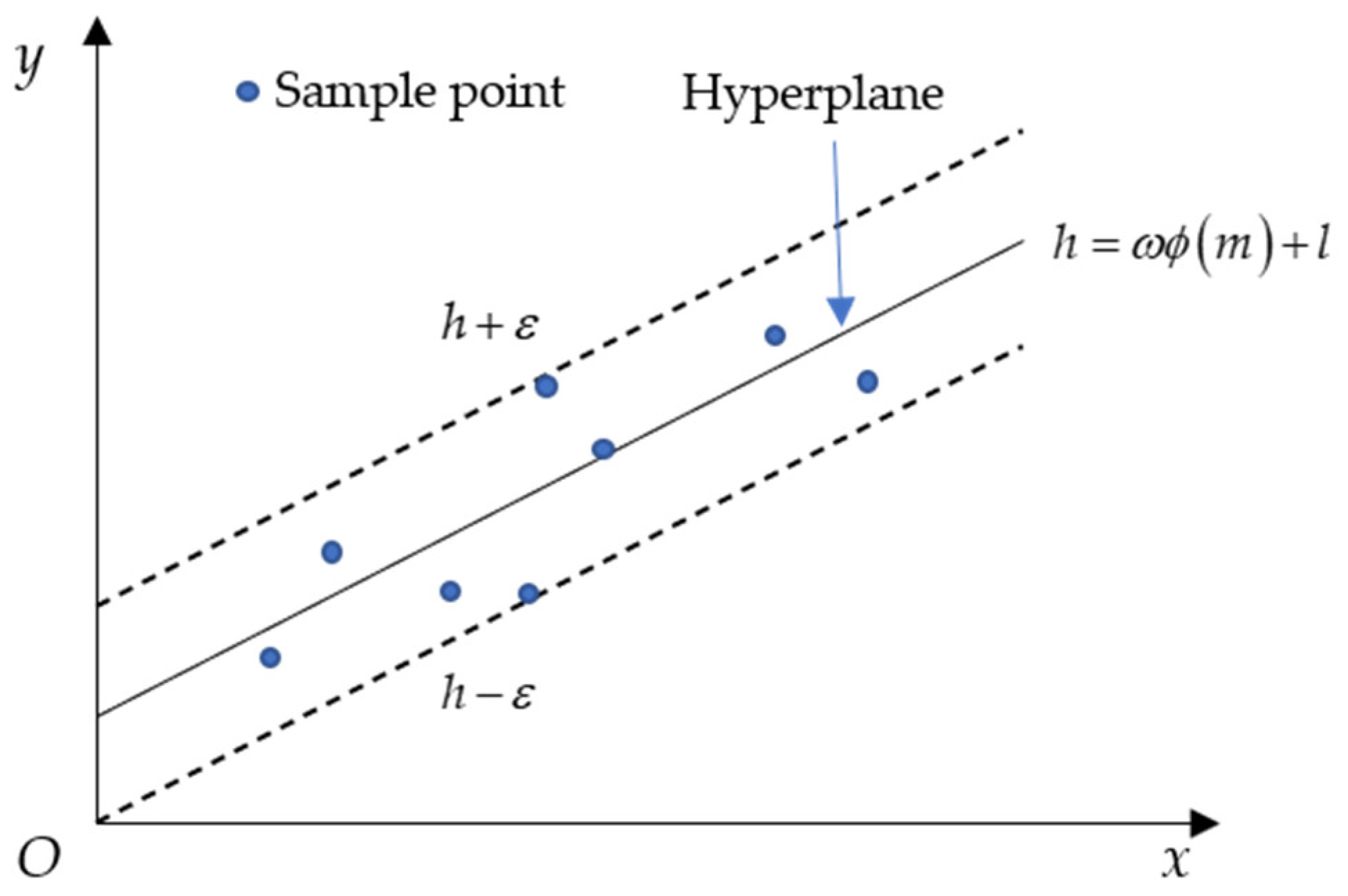
Figure 1. Hyperplane diagram.
Remotesensing 15 02188 g001
Figure 2. SGJM flow chart.
Remotesensing 15 02188 g002
Figure 3. Simulate the shape of an obstacle.
Remotesensing 15 02188 g003
Figure 4. Simulate the full tensor gravity gradient caused by obstacles.
Remotesensing 15 02188 g004
Figure 5. The relationship between detection accuracy and detection distance.
Remotesensing 15 02188 g005
Figure 6. Differential ratio dataset construction process.
Remotesensing 15 02188 g006
Figure 7. Schemes follow the same format.
Remotesensing 15 02188 g007
Figure 8. Error distribution of positioning results.
Remotesensing 15 02188 g008
Figure 9. Variation in ER and SNR with distance.
Remotesensing 15 02188 g009
Figure 10. The SGJM positioning result error: (a) Positioning error in x and y directions; (b) z-directional positioning error.
Remotesensing 15 02188 g010
Figure 11. The NRM positioning result error: (a) Positioning error in x and y directions; (b) z-directional positioning error.
Remotesensing 15 02188 g011
Figure 12. Comparison of two methods, SNR and RE: (a) SNR; (b) RE.
Remotesensing 15 02188 g012
Figure 13. Comparison of RE between NRM and SGJM.
Remotesensing 15 02188 g013
Table 1. General kernel function types and expressions.
TypeEquation
Linear K ( m i , m j ) = m i T m j
Polynomial K ( m i , m j ) = ( γ m i T m j + η ) d ,   γ > 0
Radial basis function (RBF) K ( m i , m j ) = exp ( γ | | m i m j | | 2 ) ,   γ > 0
Sigmoid K ( m i , m j ) = tanh ( γ m i T m j + η )
where γ , η , and d are kernel parameters.
Table 2. Data simulation point coordinate parameters.
AxisStart/mEnd/mStep/mHeart 1/m
x−500500100
y−500500100
z0200100
1 Obstacle material heart.
Table 3. Results of obstacle’s location.
DirectionLine 1Line 2Line 3Line 4
MAE/mRMSE/mMAE/mRMSE/mMAE/mRMSE/mMAE/mRMSE/m
x1.341.632.526.971.962.922.344.42
y2.372.845.397.582.693.671.431.80
z0.941.130.710.991.923.093.394.80
Table 4. Average relative error.
Line 1Line 2Line 3Line 4
x0.43%0.42%0.52%0.49%
y3.96%13.89%11.0%1.43%
z1.57%0.71%7.01%11.29%
Table 5. MAE and RMSE with different methods.
DirectionSGJMNRM
MAE/mRMSE/mSTD/mMAE/mRMSE/mSTD/m
x0.941.291.317.938.918.95
y1.021.511.551.091.351.37
z0.600.920.924.257.337.23
Table 6. Result of independent 2-sample t-test.
xyz
t0.780.202.08
α0.5>0.50.05
Disclaimer/Publisher’s Note: The statements, opinions and data contained in all publications are solely those of the individual author(s) and contributor(s) and not of MDPI and/or the editor(s). MDPI and/or the editor(s) disclaim responsibility for any injury to people or property resulting from any ideas, methods, instructions or products referred to in the content.