Article

Lidar Pose Tracking of a Tumbling Spacecraft Using the Smoothed Normal Distribution Transform

1
German Aerospace Center (DLR), 82234 Wessling, Germany
2
Informatics XVII-Robotics, Julius-Maximilians-Universität Würzburg, 97074 Würzburg, Germany
*
Author to whom correspondence should be addressed.
Remote Sens. 2023, 15(9), 2286; https://doi.org/10.3390/rs15092286
Submission received: 23 March 2023 / Revised: 23 April 2023 / Accepted: 24 April 2023 / Published: 26 April 2023
(This article belongs to the Special Issue Autonomous Space Navigation)

Abstract

:
Lidar sensors enable precise pose estimation of an uncooperative spacecraft in close range. In this context, the iterative closest point (ICP) is usually employed as a tracking method. However, when the size of the point clouds increases, the required computation time of the ICP can become a limiting factor. The normal distribution transform (NDT) is an alternative algorithm which can be more efficient than the ICP, but suffers from robustness issues. In addition, lidar sensors are also subject to motion blur effects when tracking a spacecraft tumbling with a high angular velocity, leading to a loss of precision in the relative pose estimation. This work introduces a smoothed formulation of the NDT to improve the algorithm’s robustness while maintaining its efficiency. Additionally, two strategies are investigated to mitigate the effects of motion blur. The first consists in un-distorting the point cloud, while the second is a continuous-time formulation of the NDT. Hardware-in-the-loop tests at the European Proximity Operations Simulator demonstrate the capability of the proposed methods to precisely track an uncooperative spacecraft under realistic conditions within tens of milliseconds, even when the spacecraft tumbles with a significant angular rate.

1. Introduction

With the increasing number of active or inactive satellites orbiting the Earth, there is a need for maintaining the space infrastructure in orbit. This maintenance can include on-orbit servicing missions designed to expand the lifetime of a satellite by repairing or refueling, or active debris removal missions to take inactive satellites which could become a threat to other spacecrafts off orbit. Such a mission was demonstrated in geostationary orbit with the “Mission-Extension Vehicle 2” [1], aiming at extending the lifetime of “Intelsat 10-02” by five years.
In this context, the target spacecraft is uncooperative and might be tumbling freely. During the far- and mid-range phase of the rendezvous, an estimation of the target’s position is sufficient to initiate the approach. However, once in close-range (typically at a relative distance below 30 m), precise relative pose estimation (position and attitude) becomes necessary in order to perform possible robotic activities such as grasping and detumbling. If visual cameras can be used for pose estimation, they are also strongly affected by the varying luminosity conditions (day/night eclipses and high contrast) [2]. On the contrary, active range imaging sensors such as lidars and time-of-flight (ToF) cameras are less affected by the illumination conditions. The use of these sensors for space rendezvous is being increasingly studied due to the advances in these sensing devices [3].
ToF cameras provide a precise and instantaneous depth image of an object, often associated with intensity or RGB information. Yet these cameras have a very limited range with a maximum working distance of around 10 m [4,5,6], so that they have to be used in conjunction with another sensor with a wider working range for complete rendezvous scenarios. In contrast, existing lidar sensors for space can work at distances of several hundred meters up to several kilometers [1,7], so they can also be used to provide distance and direction measurements in mid-range. Thus, lidar sensors are suitable for transitioning from angles-only navigation in far-range [8,9] to full pose estimation in close-range. For this reason, the use of a lidar for uncooperative pose estimation is studied in this work. Lidars also provide precise 3D scans, yet because of their relatively low framerate, they can be subject to motion blur effects. In particular, if the target spacecraft tumbles with a high velocity, this effect becomes significant.
When using 3D scans, the task of relative pose estimation is usually split in two distinct steps, pose initialization and pose tracking. Methods for pose initialization are also widely discussed in the literature [10,11,12], but this work will focus on the second part, pose tracking. Point cloud registration aims at aligning two 3D scans given an initial estimate of their relative pose. The most commonly used registration algorithm is the iterative closest point (ICP) [13]. ICP or one of its variants is generally used for tracking an uncooperative target with range imaging sensors [3]. While ICP is a precise and robust registration method, when the size of the point clouds increases, it can become difficult to perform registration in real-time [6]. This is especially true with on-board computers which have limited capabilities compared to the processing hardware available on ground.
An alternative algorithm is the normal distribution transform (NDT) [14], which was often found to be faster than ICP while reaching similar precision [15,16]. However, the NDT suffers from discontinuity issues of the cost function, making it sensitive to a good initial estimate in order to converge [17]. The main contributions of this work are the formulation of a smoothed version of the NDT aiming at tackling this issue, the investigation of different strategies for accounting for motion blur when tracking tumbling targets, and the extensive hardware-in-the-loop evaluation of these methods. In detail, a Gaussian kernel is used to smooth the NDT map and increase the algorithm’s robustness and efficiency. For performing motion blur correction of the point cloud, the first evaluated strategy consists in the use of a Kalman filter, and the second in a continuous-time formulation of the NDT registration algorithm. The different methods are evaluated experimentally and compared to ICP in hardware-in-the-loop tests for different scenarios, including cases where the target satellite tumbles with a high angular rate.
The remainder of this paper is structured as follows. In Section 2, related work and point cloud registration algorithms are described in detail. Section 3 introduces the proposed smoothed NDT algorithm as well as strategies for motion blur compensation. Hardware-in-the-loop experiments were performed to evaluate these methods for tracking uncooperative tumbling targets. They are presented in Section 4, and discussed in the following Section 5. Finally, Section 6 concludes the paper.

2. Related Work

2.1. Point Cloud Registration

Fine point cloud registration methods are local optimization methods, which rely on an initial estimate to find the relative pose between two scans. These methods are used in various fields of robotics. An extensive review of fine point cloud registration methods can be found in [17]. When using a registration method, the two scans which are matched are called the target and the source point cloud. The target point cloud is the reference or model scan, which is possibly created from a CAD model. The second scan is the source point cloud; it is often the last point cloud that was recorded by the sensor.
The most famous fine registration method is the iterative closest point (ICP), which was introduced by Besl and McKay [13]. The principle of ICP is to express the disparity between the two point clouds via a least squares formulation. For each point of the source cloud, the Euclidean distance to the closest point in the target point cloud is measured. The optimal rigid transformation that aligns both scans is found by minimizing the sum of these squared distances iteratively until convergence. There exist numerous variants of the ICP, among which are point-to-plane ICP [18], trimmed ICP [19] or generalized ICP [20]. The ICP is a highly precise registration method. Nevertheless, association mismatches can happen due to the nearest neighbor strategy [17].
A second popular algorithm is the normal distribution transform (NDT). The NDT was first introduced for 2D point clouds by Biber and Straßer [14] before being extended for 3D scans [21]. The first step of the NDT is to subdivide the scene into a regular voxel grid. For each voxel, the mean and covariance of the points of the target point cloud which fall into this cell are computed. The idea of the NDT is to assume that the points of the target point cloud follow a normal distribution in each cell. The alignment of a source point cloud is found by maximizing its likelihood according to this probability distribution. Likewise, gradient-based methods are used for finding the optimal pose iteratively. The NDT is also a high-precision registration method, and can be faster than the ICP because of the voxel-wise representation [15,16]. Instead of choosing a fixed voxel size for the NDT grid, coarse-to-fine strategies consist in computing multiple NDT runs with progressively reduced cell size [22,23]. Other approaches set the cell size to be smaller close to the origin of the sensor and coarser further away to account for the uneven density of points in the cloud [24,25]. Rather than using a voxel grid, Das and Waslander apply a clustering algorithm to define the groups of points which should be represented by a common distribution [26].
When the pose changes during the iterations of the NDT algorithm, the points of the source point cloud can be associated with a different voxel of the target cloud than previously. In consequence, the cost function of the NDT varies discontinuously. These discontinuities are more pronounced for the NDT than ICP because of the coarser voxel representation. Therefore, the NDT more than the ICP relies on a good initial estimate for finding the correct pose transform [27]. Solutions to overcome this robustness problem such as using eight overlapping voxel grids [24,28] or tri-linear interpolation between neighboring cells [15] lead to an increase in the computation time by four to eight times. Likewise, Quenzel and Behnke [25] form a Gaussian mixture representation by associating each point with the 27 surrounding voxel distributions, and incorporate additional metrics in the representation, but their method requires a GPU to run in real-time. Instead of 3D NDT distributions, it is also possible to consider planar distributions (surfels) adapted for projective data association on a GPU, and minimize the point-to-plane error [29]. However, there is a need for addressing the NDT discontinuity problem without losing the efficiency of the algorithm or requiring a GPU.
Lidar sensors are subject to motion blur or motion distortion effects, especially when dealing with fast dynamics. A common strategy to mitigate this effect is to motion compensate the point cloud in a pre-processing step based on the assumption of constant velocity and angular velocity during the scan [30,31]. In lidar odometry and mapping [32], feature-based motion estimation is performed with high frequency, before motion compensation and global registration is executed with lower frequency. Alternatively, elastic or continuous-time scan registration algorithms iteratively estimate the motion that the sensor had during the scan as part of the optimization routine [33,34,35].

2.2. Satellite Pose Tracking Using Range Data

Most authors rely on the ICP for satellite tracking with range data [4,7], or on one of its variants. Opromolla et al. use the ICP with a nearest neighbor search for the first iteration and normal shooting for the following ones [36]. Li et al. use RANSAC in combination with the ICP for robustly rejecting association mismatches and performing model-less tracking of the spacecraft using a SLAM scheme [37]. For a faster nearest neighbor search, Klionovska and Burri apply the ICP in conjunction with the reverse calibration method, meant for the registration of range images provided by ToF sensors such as PMD cameras [5]. Because ToF sensors can deliver very dense point clouds at close range, Sun et al. first extract salient points from the scan before performing ICP registration on the reduced point clouds [6]. The consecutive scans are used to increment a global map and build a model of the target spacecraft. Their approach is also compared to the classical ICP, generalized ICP and NDT, but requires high-resolution depth images. To the best of our knowledge, their work is the only one investigating the use of the NDT for satellite pose tracking reported so far, and relies on the implementation from the C++ Point Cloud Library.
Many factors can influence the quality of the point clouds: beam divergence, sensor noise, materials on the target. In particular, spacecrafts are often coated with golden multi-layer insulation (MLI) sheets, and the resulting reflections and light scattering affects the quality of the scans. To mitigate the effect of these reflections, Wang et al. use a trimmed ICP to robustly reject outliers [38]. Another effect is motion distortion, which arises when using a scanning lidar with a low acquisition frequency compared to the angular rate of the satellite (typically when the target rotates by more than a few degrees during one scan). ToF cameras are not affected by this effect due to their scanning principle, and many experimental evaluations conducted during hardware-in-the-loop experiments rely on their use [4,5,6,38]. Martinez et al. consider the problem of tracking a rocket upper-stage body spinning with a high angular rate of 10 deg/s, with simulated ToF measurements at 1 Hz [39]. For speeding up the tracking process, they combine the ICP with key-point description and matching. When using lidar simulators, motion blur is an effect which is often not modeled to generate the point clouds [36,40]. However, to account for low lidar frame-rates and the pose shift that might have happened between two scans, Opromolla and Nocerino use an unscented Kalman filter to predict the current pose of the target spacecraft [40]. The unscented filter is preferred for accounting for the non-linearities of the dynamics. The filter prediction is then used as an initial guess for ICP registration. A scanning lidar mounted on a robotic facility is used by Li et al. for estimating the pose and inertial parameters of a tumbling satellite [37]. The target satellite rotates at 1 deg/s for a scan time of 1.65 s, so that motion blur is not taken into consideration. Yin et al. conduct a hardware-in-the-loop experiment with a target tumbling with 10 deg/s, but the single-line scanning lidar that was used has an equally high acquisition frequency of 10 Hz [41]. Thus, as far as we know, the impact of motion blur when using a scanning lidar for tracking a rapidly tumbling target remains unstudied.

3. Proposed Methods

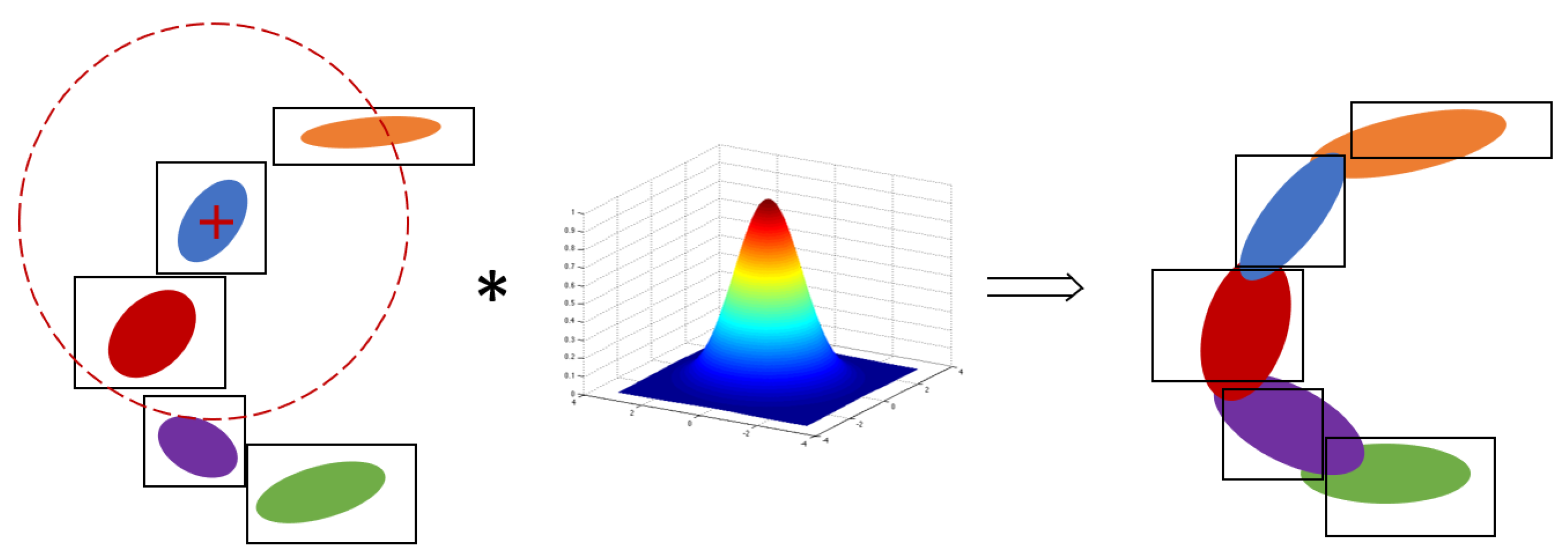
3.1. Smoothed Normal Distribution Transform

The smoothed NDT is a variant of the NDT that we introduced in [42]. It aims at mitigating the discontinuity issues of the NDT cost function mentioned in Section 2.1 without affecting the computation time of the algorithm. We will detail the main steps here. For clarity of the notation, scalars will be written in normal font, vectors in bold, and matrices in capital bold letters.
Instead of subdividing the target point cloud into a regular voxel grid (typically via an octree), the smoothed NDT relies on a kd-tree partition of the target point cloud. During construction, each cell of the tree is subdivided recursively until a minimal cell size is reached. Once the subdivision has happened, as in a standard NDT, the distribution of the points in each cell is computed. For each cell indexed by k 1 , , n , the distribution is characterized by the mean and covariance ( μ k , C k ) of the points of the target cloud belonging to that cell. Afterwards, the distributions of all cells undergo a smoothing step, so that each cell not only represents the distribution of the points it contains, but also of neighboring points.
The principle of the smoothing of a cell is presented in Figure 1. Given a certain smoothing radius, all cells within the radius are aggregated and weighted depending on their distance to the considered cell’s center. Let p be the number of distributions within the radius, which are indexed by k 1 , , k p . The new distribution obtained by aggregating theses distributions characterized by ( μ k 1 , C k 1 ) , , ( μ k p , C k p ) with the weights w k 1 , w k p is defined by the mean and covariance:
μ ˜ = i = 1 p w k i μ k i , C ˜ = i = 1 p w k i ( C k i + μ k i μ k i T ) μ ˜ μ ˜ T .
The weights are given by a continuous Gaussian blur. If c is the center of the cell being currently smoothed, then a distribution with n k i points and mean μ k i has a weight:
w k i n k i exp ( | | μ k i c | | 2 2 σ 2 ) ,
where σ is the standard deviation of the chosen Gaussian blur. It is typically chosen to be close to the minimal cell size of the kd-tree [42], while the smoothing radius for considering neighboring distributions can be chosen to equal 3 σ .
Finally, registration of a source point cloud ( z 1 , , z m ) is performed using the smoothed distributions. The homogeneous 3D transformation which aligns the source point cloud with the target point cloud is denoted by T S E ( 3 ) . In this work, the pose will be characterized by a rotation matrix and a position and will be viewed as T = ( R , p ) S O ( 3 ) × R 3 . Instead of computing the likelihood according to the normal distribution as in the classical NDT, a relaxed cost function is used to speed up the optimization process, as in [23]. The optimal pose is the one which minimizes the distance of the source point cloud to the distributions of the target point cloud in a least squares sense, according to the Mahalanobis distance between a point and a distribution:
min T i = 1 m μ ˜ η ( i ) T ( z i ) T C ˜ η ( i ) 1 μ ˜ η ( i ) T ( z i ) .
Here, η : 1 , , m 1 , , n is the mapping, such that ( μ ˜ η ( i ) , C ˜ η ( i ) ) are the smoothed distribution parameters of the cell closest to T ( z i ) . The cost function is minimized in an iterative way using weighted least squares. The gradients can be computed analytically. For a representation of the optimization problem with a minimal number of parameters, the optimization can be performed in the manifold of the Lie group S E ( 3 ) . Using the same convention as Sola et al. [43], the capitalized Exp and Log function map a vector ρ R 3 to its corresponding rotation matrix R S O ( 3 ) :
Exp ( ρ ) exp ( ρ × ) = R , Log ( R ) = ρ ,
where ρ × is the cross product matrix of ρ . The left “round-plus” operator is introduced to represent an increment of an element T = ( R , p ) of S E ( 3 ) by a vector of the manifold δ R 6 :
δ T = Exp δ 1 : 3 R , δ 4 : 6 + p .
Next, the left Jacobian on Lie groups [43] of a transformation of a point z i is defined by
J i = D T ( z i ) D T lim δ 0 ( δ T ) ( z i ) T ( z i ) δ = ( R z i ) × I 3 ,
where I 3 is the identity matrix of size 3. The justification for the last line is given in Appendix A.1. The increment to apply according to the Gauss–Newton algorithm is ϵ R 6 solution of
( i = 1 m J i T C ˜ η ( i ) 1 J i ) ϵ = i = 1 m J i T C ˜ η ( i ) 1 T z i μ ˜ η ( i ) .
Finally, the pose is updated via T ϵ T until convergence.
Compared to the classical NDT, the smoothed NDT only requires the additional smoothing step, which is performed as a pre-processing step. Because the smoothing can be performed efficiently using the tree structure, the additional computation time is minor [42]. In the case where a reference 3D model of the satellite is known beforehand, the construction of the smoothed NDT map only has to be performed once with this model point cloud. Each incoming source point cloud is then registered with respect to this smoothed NDT map.

3.2. Conjunction with a Filter and Motion Compensation

In its basis configuration, the tracking always uses the previous NDT result as an initial guess for estimating the pose of the current scan. The principle of this tracking method is summarized in Figure 2.
When the lidar frame-rate is low, or the relative dynamics is fast, this initial guess might be inaccurate. A more precise initial estimate can be obtained by using the prediction from a navigation filter as an initial estimate, whether it is with a simple kinematic-only filter [36] or a more complex unscented filter [40]. Similarly to [36], we use a simple filter to estimate the current velocity and angular velocity of the target satellite. The currently estimated position and velocity of the target with respect to the chaser are denoted by p k and v k . The predictions at the next time step after time Δ t are denoted by the subscript k + 1 | k . Under a simple assumption of constant relative velocity, they yield
p k + 1 | k = p k + v k Δ t v k + 1 | k = v k .
The attitude of the target in the chaser coordinate frame is R k , and ω k is the angular velocity expressed in the target coordinate frame. The prediction according to a simplified model of constant angular velocity is
R k + 1 | k = R k Exp ( ω k Δ t ) ω k + 1 | k = ω k .
This basic evolution model of the relative dynamics is sufficient for the purpose of this filter, which is only to support the pose estimation. Moreover, it does not require knowledge of the target’s inertial parameters. For the guidance and control tasks, a separate and more complex filter can be used, but is not the subject of this work.
The NDT algorithm provides a pose measurement ( R ¯ k + 1 , p ¯ k + 1 ) which is used to update both Kalman filters. The position filter is a linear Kalman filter. Given the state and measurement noises, the gain K k + 1 p o s R 6 × 3 is obtained by the standard Kalman filter theory, and is used to perform the update:
p k + 1 v k + 1 = p k + 1 | k v k + 1 | k + K k + 1 p o s ( p ¯ k + 1 p k + 1 | k ) .
For the attitude, an invariant extended Kalman filter (IEKF) [44] is used, as it is an elegant generalization of extended Kalman filtering on Lie groups. Similarly to an extended Kalman filter, the IEKF theory provides a gain K k + 1 a t t R 6 × 3 which is used to update the attitude prediction. We refer to [44,45] for a detailed description of the IEKF equations. The increment in the attitude space is performed using the ⊕ operator of Equation (5):
( R k + 1 , ω k + 1 ) = K k + 1 a t t Log ( R ¯ k + 1 R k + 1 | k T ) ( R k + 1 | k , ω k + 1 | k ) .
In addition to providing an initial guess for the registration algorithm, the predictions of the filter can be used to perform motion compensation of the point cloud. Motion compensation is the process of correcting the point cloud using the individual timestamp of each point in order to mitigate the effects of motion blur. In detail, each point z i of a new point cloud has a timestamp t i [ t k , t k + 1 ] , where t k and t k + 1 are the start and end times of the scan. The point cloud is motion compensated to transform all points to the position they would have at the end of the scan. Calling Δ t i = t k + 1 t i , each point expressed in the chaser coordinate frame is transformed according to the linear kinematics model of Equations (8) and (9):
z i ( t k + 1 ) = p k + 1 | k + Exp ( R k ω k Δ t i ) ( z i ( t i ) p k + 1 | k + v k Δ t i ) ,
where R k ω k is the angular velocity expressed in the chaser coordinate frame. This motion compensation can be performed as a pre-processing step of the raw point clouds prior to performing registration. It is computationally inexpensive compared to the registration algorithm. The overall tracking logic when using the filter prediction and performing motion compensation in conjunction with smoothed NDT registration is presented in Figure 3.

3.3. Continuous-Time NDT

An alternative solution to account for motion blur is the use of a continuous-time registration algorithm, for which not only the points’ position, but also their timestamp is considered during the optimization. The proposed continuous-time approach is similar to Elastic Lidar Fusion [33], but differs in that we use the smoothed NDT as an underlying registration algorithm and provide an analytical formula for the computation of the gradients.
We consider a start pose T s at time t s , and an end pose T e at time t e . The poses are characterized by the rotation matrices R s , R e S O ( 3 ) and the positions p s , p e R 3 . The interpolated pose at time t [ t s , t e ] is given by the position and attitude
p u = ( 1 u ) p s + u p e R u = Exp u Log R e ( R s ) 1 R s ,
where u = t t s t e t s is the interpolation factor. The second expression is simply the matrix formulation of the spherical linear interpolation (slerp).
Given a source point cloud ( z 1 , , z m ) with timestamps t i [ t s , t e ] , the objective of the continuous-time NDT is to find the end pose T e solution of
min T e i = 1 m μ ˜ η ( i ) T i ( z i ) T C ˜ η ( i ) 1 μ ˜ η ( i ) T i ( z i ) .
This formulation is very close to the one of the smoothed NDT (Equation (3)) with the difference that T i is the pose interpolated between T s and T e at time t i , according to Equation (13), which we write T i = interp ( T s , T e , u ) . The optimization of the end pose T e is performed in the same way as described in Section 3.1, using the Jacobian of the interpolated transformation of a point z i which is given by
J i = D interp ( T s , T e , u ) ( z i ) D T e = ( R u z i ) × u D exp ( u Log Q ) D log ( Q ) u I 3 ,
where Q = R e ( R s ) 1 , and D exp and D log are the derivation of the matrix exponential and logarithm in the tangent space of S O ( 3 ) , as given in [46]. The justification for obtaining this Jacobian is provided in Appendix A.2.
Note that in this formulation, the start pose T s is fixed and typically the result of the registration at the previous step. For accounting for high frequency motion, it is possible to relax this constraint [35], and to simultaneously optimize both poses T s and T e . However, this involves optimizing more parameters, and was found to be less stable in our experiments.
An important point usually performed as a pre-processing step for all registration algorithms is to start with a down-sampling of the point cloud using a regular voxel grid, not only to limit the point cloud size, but also to have a more even partition of the points, independently of the sensor’s scanning pattern. When down-sampling before using a continuous-time algorithm, it is important not to lose the timestamp information. We choose to set the timestamp of each down-sampled point according to the mean of the timestamps of the points which fell into that voxel. For better stability, the filter prediction can also be used as an initial guess when using the continuous-time formulation of the smoothed NDT. The resulting logic is presented in Figure 4.

4. Experimental Results

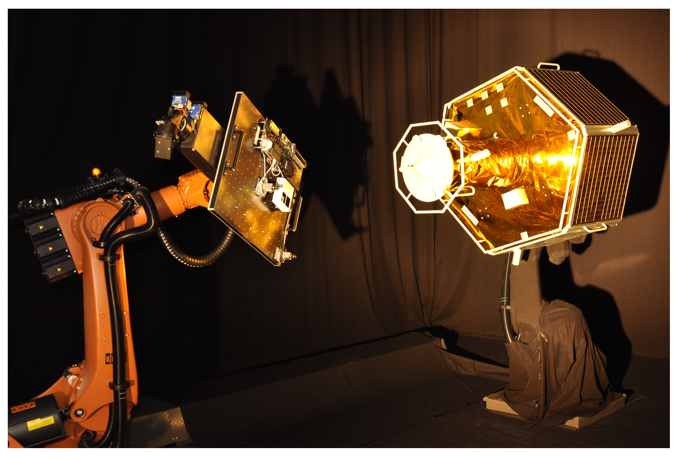
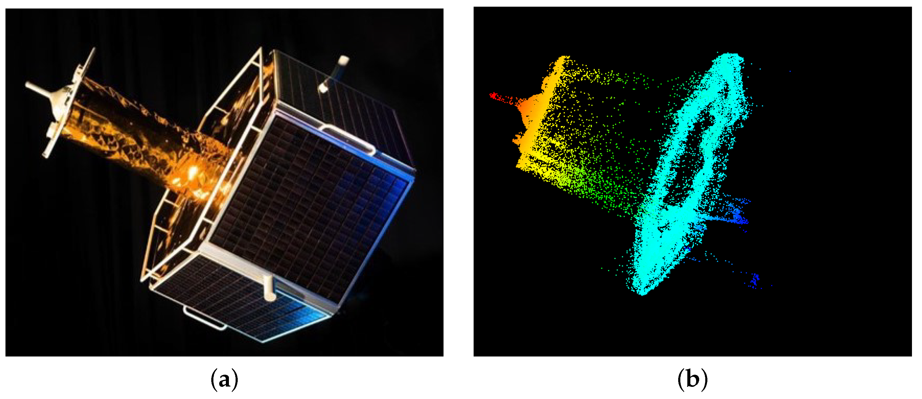
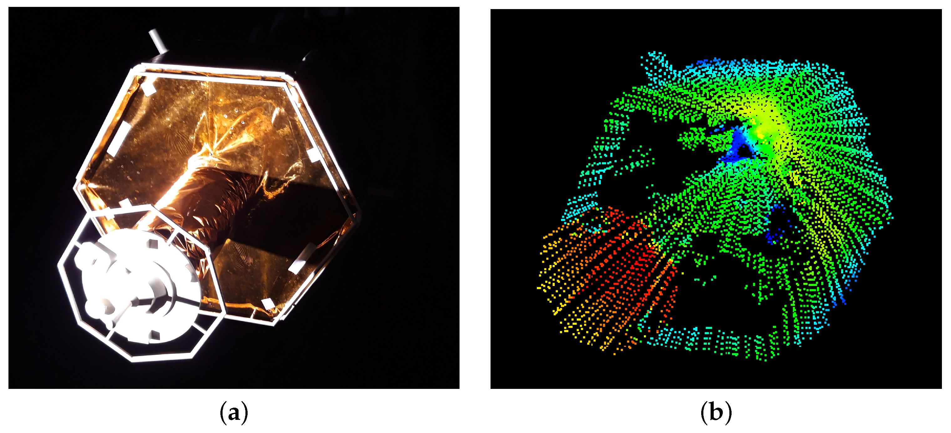
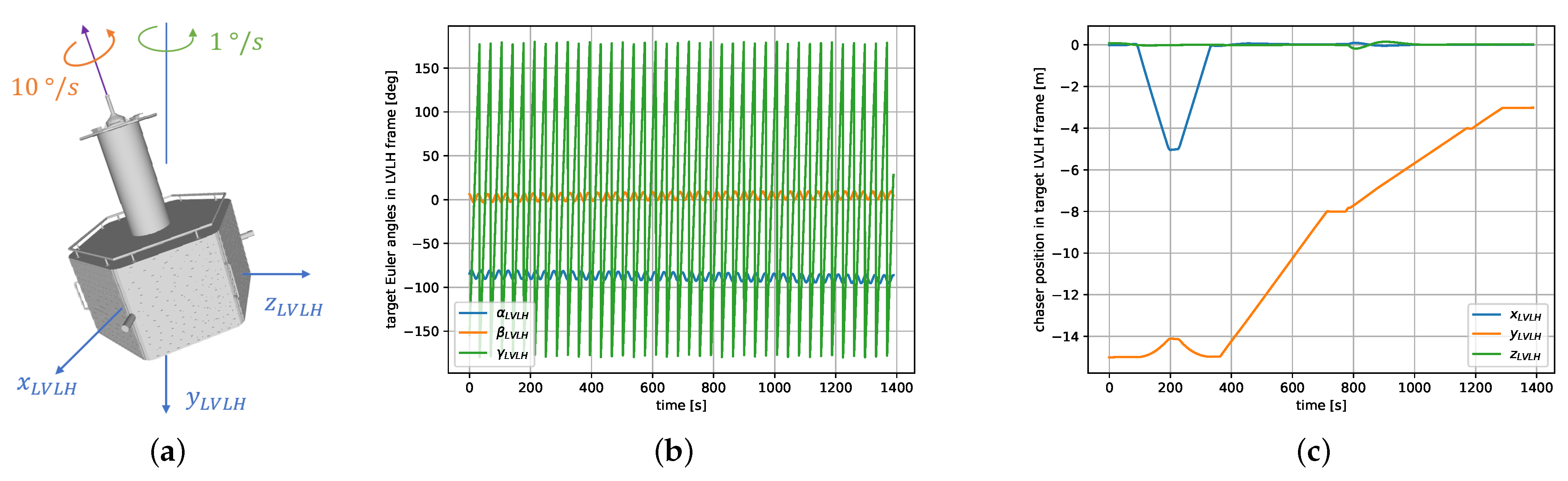
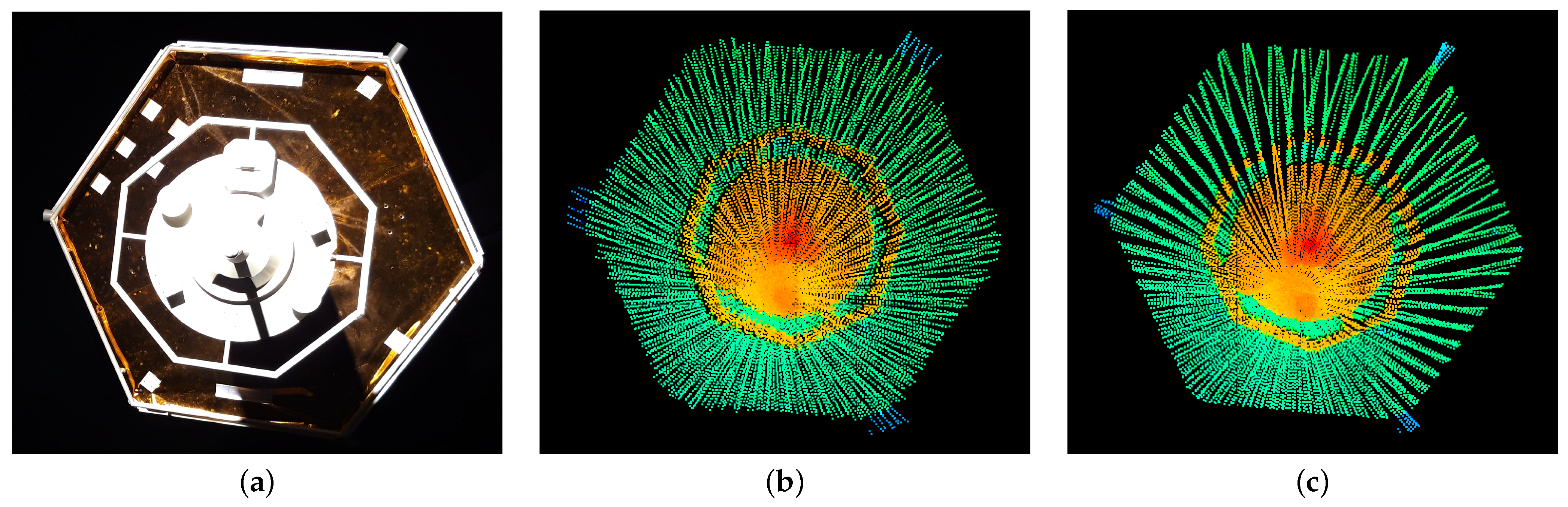
4.1. Hardware-in-the-Loop Experiments at the European Proximity Operations Simulator

The European Proximity Operations Simulator (EPOS) [47] is a hardware-in-the-loop test facility located at the German Space Operations Center (GSOC). The facility consists of two robotic arms which can move with 6DOF, as shown in Figure 5. One of the robotic arms is additionally mounted on a linear rail, so that relative motions can be simulated up to a relative distance of 25 m. A spotlight simulates sun light. For these experiments, a true scale mockup of the DEOS (Deutsche Orbitale Servicing Mission) satellite project was used. This mockup is made of realistic materials, such as the solar panels and the golden multi-layer insulation (MLI) sheets.
For the experiments, a lidar sensor from the automotive domain (Livox® Mid-40) was used. Because the lidar also captures points from the test facility which would not be observed in space (robotic arm, floor, curtains in the background…), points which do not belong to the spacecraft mockup are cropped out from the point cloud in a pre-processing step. The point clouds captured by the lidar are very noisy. A first cause for erroneous points is the effect of beam divergence, which is illustrated in Figure 6. Due to the high reflectivity of the MLI, whenever the orientation of the sheets is not perpendicular to the sensor, the surface becomes invisible or displays reflected points, as shown in Figure 7. This sensor also has a non-repetitive scanning pattern, so that the sampling frequency of the point clouds can be chosen in order to have a good trade-off between the density of the point clouds, and the frequency of the acquisition of new data. For the experiments, a constant acquisition frequency of 1 Hz was set.
The EPOS facility is commanded by a space dynamics simulator which calculates the dynamics of both satellites. A GNC system is also integrated in closed loop, so that maneuvers are commanded in real-time to follow the desired rendezvous approach. The point cloud processing presented in this work is integrated within this GNC system, so that the rendezvous can be performed solely with the lidar, or by fusing the measurements from multiple sensors (for instance lidar and camera) [48].

4.2. Evaluated Methods

We propose to compare the smoothed NDT, smoothed NDT with motion compensation, and continuous-time NDT for lidar-based tracking of a satellite in close range. Given a CAD model of the target, a point cloud model of the target is constructed, against which the real point clouds captured by the sensor are matched. We additionally compare our methods with a state-of-the-art implementation of the ICP given by the 3D toolkit [49]. The ICP is compared with the smoothed NDT in its basic functioning, meaning that the previous result of the registration is used as initial estimate whenever a new point cloud is received, as in the configuration described in Figure 2. To distinguish between the different variants that are compared, we will refer to the different algorithms by the following:
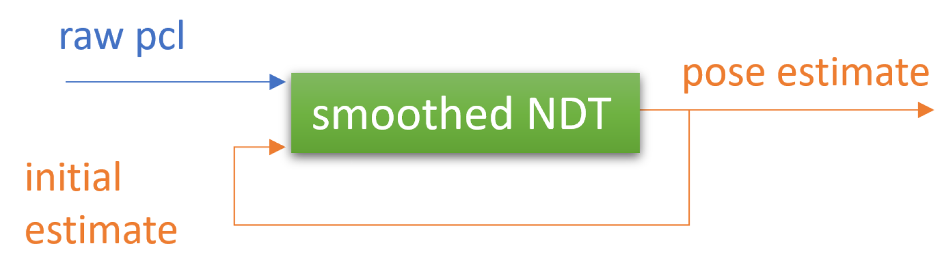
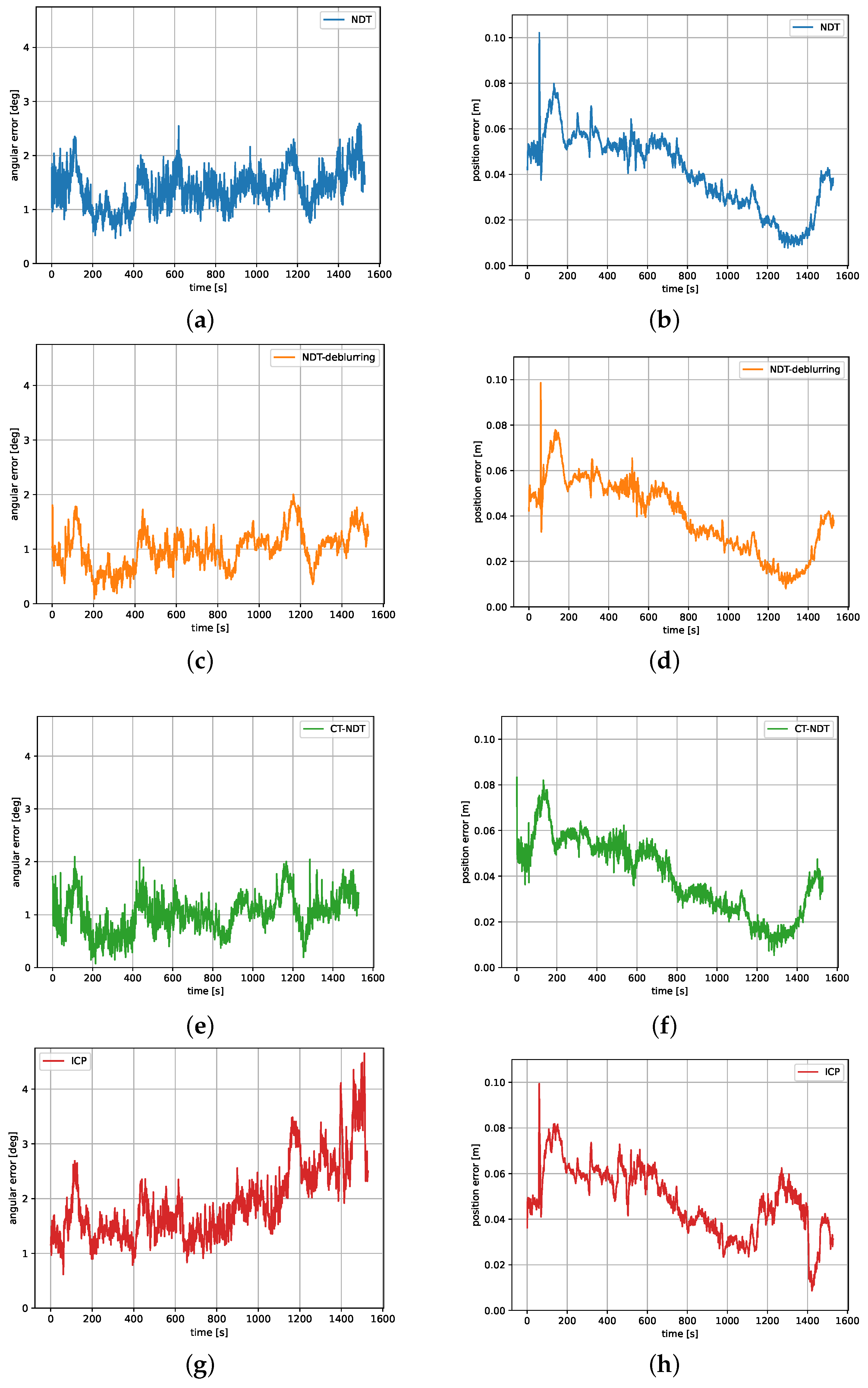
  • NDT: Smoothed NDT as presented in Section 3.1, with simple feedback as in Figure 2;
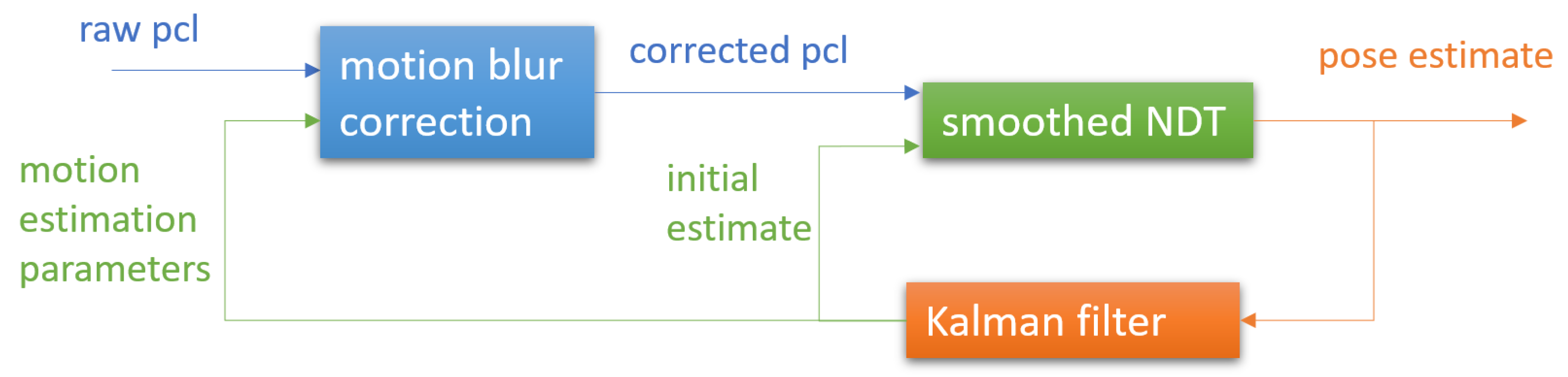
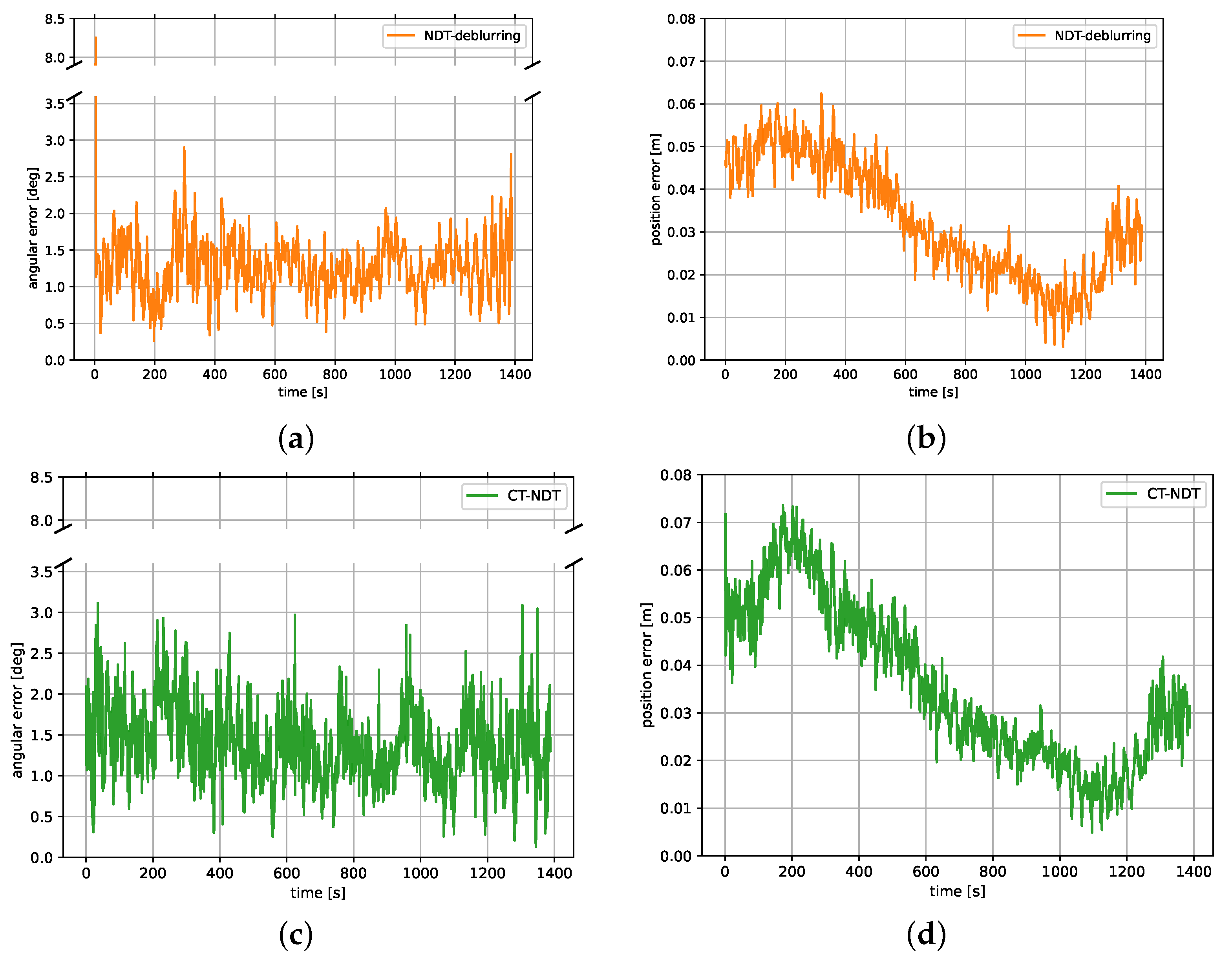
  • NDT-deblurring: Smoothed NDT with motion compensation as in Section 3.2, in conjunction with the Kalman filter as in Figure 3;
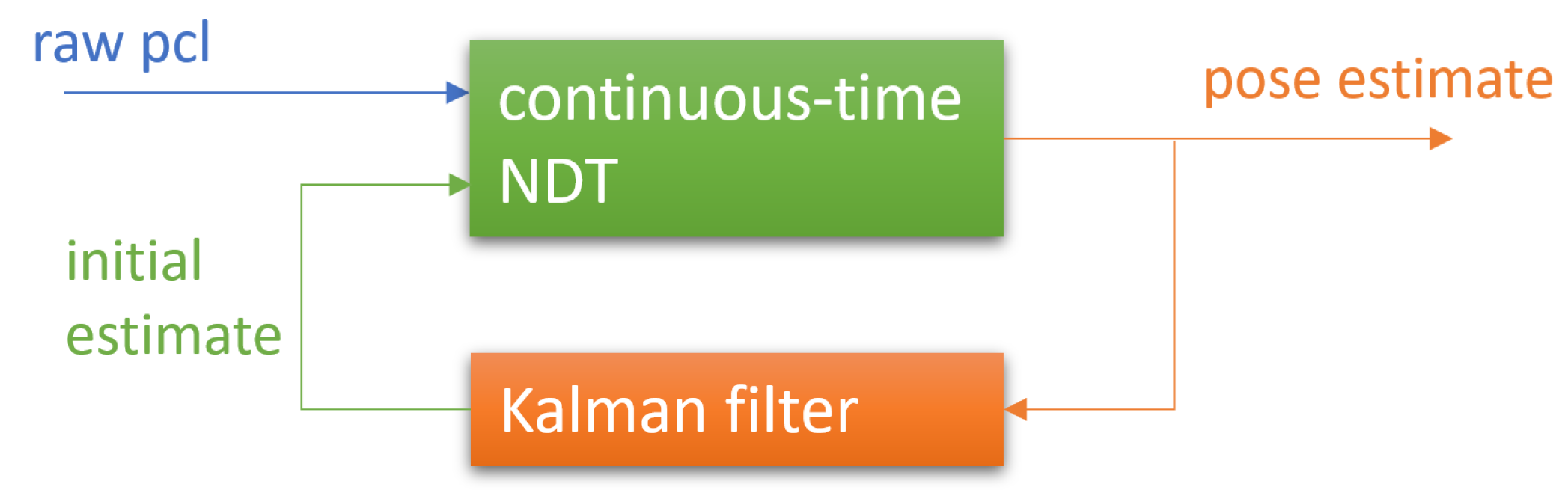
  • CT-NDT: Continuous-time smoothed NDT presented in Section 3.3, in conjunction with the Kalman filter as in Figure 4;
  • ICP: Implementation of ICP from the 3D toolkit, with simple feedback as in Figure 2.
The same parameters were used for the three different NDT-based methods for both experiments, and are presented in Table 1. For the ICP, these parameters had to be adapted in order to achieve better precision. The maximum number of iterations was also doubled with respect to the NDT, at the expense of longer processing times, but these iterations are needed by the algorithm in order to converge to the correct estimation. The different methods were implemented in C++, and the processing times were all evaluated on one core of an Intel Core i7 CPU.

4.3. Hardware-in-the-Loop Results for a Slowly Spinning Target

The first experiment performed at EPOS consisted of an inspection and rendezvous scenario at a distance of 15 m to 3 m from the target satellite. When the relative distance of the center of mass of both satellites was 3 m, the distance to the target’s surface was smaller (around 1.5 m), so that at this distance, servicing or de-orbiting operations could take place.
The local vertical, local horizontal (LVLH) frame of the target spacecraft was used to represent the rendezvous trajectory. During the whole experiment, the target spun freely around the y L V L H axis at 1 ° / s, as represented in Figure 8a,b. The rendezvous was divided in several parts, and started at a relative distance of 15 m from the target, as depicted in Figure 8c. In the first phase (until t = 500 s), an inspection trajectory was flown to view the target from different sides, at a steady distance of 15 m. Once the initial hold point was reached again, the approach started along the y L V L H direction. The first approach from 15 m to 8 m (for t [ 550 s , 900 s ] ) was performed with a velocity of 2 cm/s, and the following approach from 8 m to 3 m (for t [ 970 s , 1470 s ] ) was conducted at 1 cm/s.
The whole experiment lasted about 27 min, during which the lidar was operated at 1 Hz. The trajectory was flown in a closed loop with the GNC system relying solely on the lidar NDT pose tracking. At the start of the experiment, the tracking was initialized with the target’s ground truth pose. The original point clouds contained between 8000 and 70,000 points, depending on the relative distance to the target. After applying a voxel filter with a grid size of 2 cm, the down-sampled point clouds contained between 6000 and 15,000 points.
While the trajectory was flown in a closed loop with the GNC system, to compare the different variants, the results were reproduced in an open loop after the experiment with the saved point clouds. The results of the pose tracking during the rendezvous for the four algorithms are presented in Figure 9.
For each algorithm, the total attitude and position error compared to the ground truth given by the facility is presented. The position error is defined as the distance between the true and estimated position of the target’s center of mass in the chaser frame. The total attitude error is defined to be the angle (as in the axis-angle representation) describing the magnitude of the rotation between the true and estimated attitude.
If the translation errors of all algorithms are similar, the angular errors differ between the methods. The maximal angular error over the approach for the NDT (Figure 9a) is 2 . 6 ° , while it is 2 ° for NDT-deblurring (Figure 9c) and 2 . 1 ° for the CT-NDT (Figure 9e). For the ICP, the maximal angular error is 4 . 7 ° (Figure 9g). These results, as well as the average and maximum values of the execution times and number of iterations for each algorithm, are summarized in Table 2. The execution times comprise the full processing of a point cloud, meaning the down-sampling via the voxel filter and the registration.

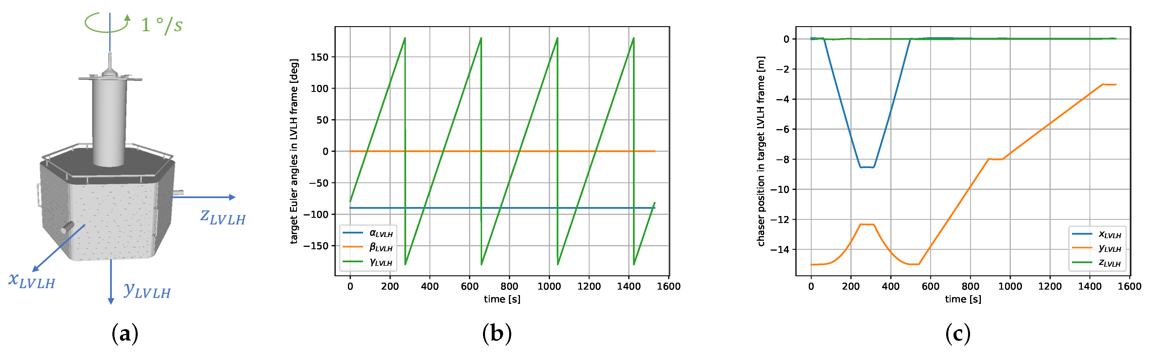
4.4. Hardware-in-the-Loop Results for a Rapidly Tumbling Target

In the second experiment, the rendezvous trajectory was similar to the previous experiment (Section 4.3), but the target spacecraft had a much faster tumbling motion. This time, the target spacecraft had an inertia matrix which was not proportional to identity, which led to the tumbling. The inertial term corresponding to the spinning axis of the target satellite was 1.2 times higher than the two other terms. This real inertia of the target was unknown to the simple Kalman filter presented in Section 3.2, which assumes a constant angular velocity, and thus assumes an inertia matrix proportional to identity. The real inertia matrix was not used in the filter in order to test the robustness of the method in the case where the inertial parameters are unknown (or only known approximately).
The tumbling movement of the target is illustrated in Figure 10a,b. The satellite spins at 10 ° /s, in coordination with a precession movement of 1 ° /s. The maximum angular displacement between the y L V L H axis and the target’s main spinning axis is around 10 ° . The rendezvous trajectory is represented in Figure 10c. The fly-around and inspection of the target at a relative distance of 15 m ends at t = 350 s. Afterwards, the initial approach up to 8 m with a velocity of 2 cm/s is performed until t = 700 s. The final approach up to 3 m is flown at 1 cm/s, with an intermediary stop at a distance of 4 m at t = 1150 s.
The 23-minute-long rendezvous was successfully performed in a closed loop based solely on the lidar pose estimation using the NDT-deblurring method of Section 3.2. Again, the pose tracking was initialized at the beginning of the experiment with the ground truth pose, and the lidar framerate was 1 Hz. When testing the smoothed NDT and ICP algorithms on the data collected during this experiment, the tracking failed. Thus, only the results for the NDT-deblurring and CT-NDT algorithms are presented in Figure 11.
Table 3 summarizes the results of each algorithm in terms of precision, and compares the execution times and number of iterations of both.

5. Discussion

5.1. Comparison of the Different Methods for Tracking a Slowly Spinning Target

For the first experiment, all four methods (NDT, NDT-deblurring, CT-NDT and ICP) were capable of tracking the pose of the target without drifting away (Figure 9). In terms of angular precision, the three NDT-based methods are quite similar, with NDT-deblurring being the most precise method, followed closely by the CT-NDT and smoothed NDT. On the other hand, the ICP showed good results during the fly-around phase, but the precision of the attitude tracking degraded during the following approach, making it less suitable for use in this scenario. This could be explained by the fact that when the relative distance decreases, the point clouds become denser and noisier. The ICP is a point-based method, so compared to the voxel-based representation of the NDT, it might be more affected by the high amount of noise and outliers in the point clouds at close range.
The position tracking error was very similar for all algorithms in the first experiment (Figure 9). The overall error was below 10 cm in the beginning, when the relative distance was still 15 m. During the approach, the position error decreased to reach around 4 cm only in close range. The fact that the position tracking error decreased during the approach could be induced by slight errors in the sensor calibration, and differences between the real satellite mockup and the provided CAD model.
At t = 80 s, the inspection trajectory started (Figure 8c), leading to a change in the chaser’s orientation. This “nodding" of the chaser at a relative distance of 15 m led to a relatively high-frequency relative translation movement of the target satellite, leading to a spike in the position error, which can be observed in Figure 9b,d,h. Interestingly, this spike was not observed for the continuous-time NDT (Figure 9f), because the method is able to correct the motion-blurred point cloud without prior knowledge on the relative dynamics.
Additionally to being more precise, the NDT-based methods largely outperform ICP in terms of efficiency (Table 2). The NDT-unblurring method is the fastest with a mean execution time of 22 ms, including the down-sampling of the point clouds. This is due to the fact that using the filter prediction as an initial guess is more precise than using the previous estimate, leading to a faster convergence and a reduced number of iterations compared to the smoothed NDT. The smoothed NDT requires 35 ms on average, and the CT-NDT comes with a higher average cost of 42 ms due to the more complex optimization process. With such execution times, all three methods are suited for efficient point cloud tracking with a high frequency. In comparison, the mean execution time of the ICP was 174 ms for this experiment. This difference can also be explained by the number of iterations of each algorithm (Table 2). All three NDT-based methods require only a few iterations in order to converge, on average below 10. The maximum number of iterations was set to 20 but is rarely reached. On the contrary, the maximum number of iterations for the ICP was set to 40, but the mean number of iterations of 32.7 indicates that this number of iterations is often needed by the algorithm.

5.2. Comparison of the Different Methods for Tracking a Rapidly Tumbling Target

For the second experiment, the smoothed NDT and ICP method did not enable the successful tracking of the target over the whole approach, as the attitude estimation was not able to cope with the fast tumbling movement between two consecutive scans. The target having multiple symmetry axes (hexagonal shape as can be seen in Figure 12a) during the frontal approach, these algorithms would jump by 60 ° in terms of attitude error. On the contrary, the two strategies developed for mitigating the effects of motion blur (NDT-deblurring and CT-NDT) were successful and enabled the tracking of the target over the whole rendezvous. Because of the fast dynamics of the target, motion blur is visible on the point clouds, and the motion compensation enables the reconstruction of more precise point clouds, as shown in Figure 12.
Concerning the errors of both methods, the first striking observation that can be made in Figure 11a is that the initial attitude error of the NDT-deblurring tracking is high. The error initially goes up until 8 . 3 ° , before it decreases and stays below 3 ° for the rest of the experiment. The reason for this spike is that the filter, which is used for motion compensating the point clouds, is un-initialized in the beginning and assumes a zero angular velocity of the target. After the first observations, it converges to estimate the real angular velocity of the tumbling spacecraft, so that the point clouds are correctly un-distorted. This spike is inevitable, yet only observed at initialization. Depending on the rendezvous scenario, this initial convergence time might not be problematic. On the contrary, the CT-NDT only relies on the filter for providing an initial guess, but is able to motion compensate the point clouds as part of the optimization process, which is why no convergence phase is observed. The total angular error stays below 3 . 1 ° during the rendezvous as illustrated in Figure 11c.
The position errors of the NDT-deblurring and CT-NDT methods were again quite similar for both experiments (Figure 11b,d). The position error decreased to a few cm at the end of the rendezvous. Their similar shape over time indicate that both algorithms might be affected by the same biases, probably calibration errors and mismatches between the CAD model and real mockup. As for the first experiment, Table 3 indicates that NDT-deblurring is faster on average than the CT-NDT. The mean total execution time for NDT-deblurring is 26 ms versus 47 ms for the CT-NDT. Both algorithms terminated within a few iterations. NDT-deblurring is faster and slightly more precise, which is why it might be preferred over the CT-NDT if the requirements of timing are a main driver. On the contrary, the CT-NDT appears to be more robust to unexpected dynamics and relatively independent of the filter convergence times.

6. Conclusions

In this work, we applied a smoothed formulation of the NDT to the problem of lidar-based tracking of a tumbling spacecraft for proximity operation scenarios. For mitigating the effects of motion blur inherent to lidar sensors when tracking a rapidly tumbling target, two strategies were proposed. The NDT-deblurring strategy consists in motion-compensating the point clouds via a simple Kalman filter. Additionally, for speeding up the registration process, the filter prediction can be used as an initial estimate. The second strategy, the CT-NDT, is a continuous time formulation of the smoothed NDT algorithm aiming at performing motion compensation of the point cloud as part of the optimization process, by making use of the individual timestamps of each point. The algorithms were tested during hardware-in-the-loop experiments in two scenarios, and compared to a standard ICP implementation. When tracking a slowly spinning target, the three NDT-based methods achieve better precision and efficiency than the ICP, and terminate within tens of milliseconds. The added value of the motion compensation strategies is demonstrated when tracking a rapidly tumbling target. Both the NDT-deblurring and CT-NDT methods enable efficient and precise tracking of the target with errors below a few degrees and a few centimeters.
All three proposed NDT-based methods are suited for on-board implementation due to their precision and efficiency. If the considered target spacecraft has a fast tumbling motion, the NDT-deblurring and CT-NDT strategies ensure that the precision of the tracking is not affected by the sensor’s motion blur. Both strategies enable the successful tracking of a tumbling target, even when the lidar framerate is low. If NDT-deblurring is slightly faster, the CT-NDT was shown to be slightly more robust to unknown dynamics.
Nevertheless, all proposed methods rely on an initial estimate at the beginning of the tracking in order to be initialized. Future work will include the development of a pose initialization algorithm to be used in coordination with the proposed tracking methods. In addition, for being closer to real space conditions, future experiments will be conducted on realistic space computing hardware, and might include a lidar sensor designed for use in space.

Author Contributions

Conceptualization, methodology and software, L.R.; preparation of the experiments, L.R. and H.F.; writing—original draft preparation, L.R.; writing—review and editing, H.F. and A.N.; supervision, A.N. All authors have read and agreed to the published version of the manuscript.

Funding

This research received no external funding.

Data Availability Statement

The research data is not publicly available due to internal restrictions.

Conflicts of Interest

The authors declare no conflict of interest.

Appendix A. Jacobians of the NDT Cost Function

Appendix A.1. Jacobian for the Classical Formulation

By definition of the left Jacobians on Lie groups [43], we have for R S O ( 3 ) and z R 3
D ( R z ) D R = lim τ 0 exp ( τ × ) R z R z τ ,
where τ R 3 . Using the Taylor expansion
exp ( τ × ) = I 3 + τ × + o ( τ ) ,
the derivative re-writes
D ( R z ) D R = lim τ 0 τ × R z τ = ( R z ) × .

Appendix A.2. Jacobian for the Continuous-Time Formulation

We use again the definition of the left Jacobians on Lie groups [43] to define the derivative of the exponential map of x R 3
D exp ( x ) = D Exp ( x ) D x = lim τ 0 Log Exp ( x + τ ) Exp ( x ) 1 τ .
Likewise, the derivative of the logarithm map of M S O ( 3 ) is defined by
D log ( M ) = D Log ( M ) D M = lim τ 0 Log Exp ( τ ) M Log ( M ) τ .
The analytical expression of these two derivatives is given by Eade [46].
Using the chain rule on Lie groups [43], the left Jacobian on Lie groups of the interpolated attitude with respect to the end attitude is
D R u D R e = D Exp u Log Q R s D R e = D Exp ( u Log Q ) D R e ( using the limit definition ) = D Exp ( u Log Q ) D ( u Log Q ) D ( u Log Q ) D Q D Q D R e ( chain rule ) = D exp ( u Log Q ) u D log ( Q ) D R e ( R s ) 1 D R e ( definition of Q ) = D exp ( u Log Q ) u D log ( Q ) ( using the limit definition ) .
Finally, using the chain rule, the derivative of the interpolated rotation evaluated at point z i is
D ( R u z i ) D R e = D ( R u z i ) D R u D R u D R e = ( R u z i ) × u D exp ( u Log Q ) D log ( Q ) .

References

  1. Pyrak, M.; Anderson, J. Performance of Northrop Grumman’s Mission Extension Vehicle (MEV) RPO imagers at GEO. In Proceedings of the Autonomous Systems: Sensors, Processing and Security for Ground, Air, Sea and Space Vehicles and Infrastructure 2022, Orlando, FL, USA, 6 June 2022; Volume 12115, pp. 64–82. [Google Scholar] [CrossRef]
  2. Cassinis, L.P.; Fonod, R.; Gill, E. Review of the robustness and applicability of monocular pose estimation systems for relative navigation with an uncooperative spacecraft. Prog. Aerosp. Sci. 2019, 110, 100548. [Google Scholar] [CrossRef]
  3. Opromolla, R.; Fasano, G.; Rufino, G.; Grassi, M. A review of cooperative and uncooperative spacecraft pose determination techniques for close-proximity operations. Prog. Aerosp. Sci. 2017, 93, 53–72. [Google Scholar] [CrossRef]
  4. Liu, L.; Zhao, G.; Bo, Y. Point cloud based relative pose estimation of a satellite in close range. Sensors 2016, 16, 824. [Google Scholar] [CrossRef]
  5. Klionovska, K.; Burri, M. Hardware-in-the-Loop Simulations with Umbra Conditions for Spacecraft Rendezvous with PMD Visual Sensors. Sensors 2021, 21, 1455. [Google Scholar] [CrossRef]
  6. Sun, D.; Hu, L.; Duan, H.; Pei, H. Relative Pose Estimation of Non-Cooperative Space Targets Using a TOF Camera. Remote Sens. 2022, 14, 6100. [Google Scholar] [CrossRef]
  7. Ruel, S.; Luu, T.; Berube, A. Space shuttle testing of the TriDAR 3D rendezvous and docking sensor. J. Field Robot. 2012, 29, 535–553. [Google Scholar] [CrossRef]
  8. Gaias, G.; D’Amico, S.; Ardaens, J.S. Angles-only navigation to a noncooperative satellite using relative orbital elements. J. Guid. Control Dyn. 2014, 37, 439–451. [Google Scholar] [CrossRef]
  9. Sullivan, J.; Koenig, A.; D’Amico, S. Improved maneuver-free approach to angles-only navigation for space rendezvous. In Proceedings of the 26th AAS/AIAA Space Flight Mechanics Meeting, Napa, CA, USA, 14–18 February 2016. [Google Scholar]
  10. Opromolla, R.; Fasano, G.; Rufino, G.; Grassi, M. A model-based 3D template matching technique for pose acquisition of an uncooperative space object. Sensors 2015, 15, 6360–6382. [Google Scholar] [CrossRef]
  11. Klionovska, K.; Benninghoff, H. Initial pose estimation using PMD sensor during the rendezvous phase in on-orbit servicing missions. In Proceedings of the 27th AAS/AIAA Space Flight Mechanics Meeting, San Antonio, TX, USA, 5–9 February 2017. [Google Scholar]
  12. Guo, W.; Hu, W.; Liu, C.; Lu, T. Pose initialization of uncooperative spacecraft by template matching with sparse point cloud. J. Guid. Control Dyn. 2021, 44, 1707–1720. [Google Scholar] [CrossRef]
  13. Besl, P.J.; McKay, N.D. Method for registration of 3-D shapes. In Proceedings of the Sensor Fusion IV: Control Paradigms and Data Structures, Boston, MA, USA, 12–15 November 1991; Volume 1611, pp. 586–606. [Google Scholar] [CrossRef]
  14. Biber, P.; Straßer, W. The normal distributions transform: A new approach to laser scan matching. In Proceedings of the 2003 IEEE/RSJ International Conference on Intelligent Robots and Systems (IROS 2003) (Cat. No. 03CH37453), Las Vegas, NV, USA, 27–31 October 2003; Volume 3, pp. 2743–2748. [Google Scholar] [CrossRef]
  15. Magnusson, M.; Nuchter, A.; Lorken, C.; Lilienthal, A.J.; Hertzberg, J. Evaluation of 3D registration reliability and speed-A comparison of ICP and NDT. In Proceedings of the 2009 IEEE International Conference on Robotics and Automation, Kobe, Japan, 12–17 May 2009; pp. 3907–3912. [Google Scholar] [CrossRef]
  16. Pang, S.; Kent, D.; Cai, X.; Al-Qassab, H.; Morris, D.; Radha, H. 3d scan registration based localization for autonomous vehicles–A comparison of ndt and icp under realistic conditions. In Proceedings of the 2018 IEEE 88th Vehicular Technology Conference (VTC-Fall), Chicago, IL, USA, 27–30 August 2018; pp. 1–5. [Google Scholar] [CrossRef]
  17. Dong, Z.; Liang, F.; Yang, B.; Xu, Y.; Zang, Y.; Li, J.; Wang, Y.; Dai, W.; Fan, H.; Hyyppä, J.; et al. Registration of large-scale terrestrial laser scanner point clouds: A review and benchmark. ISPRS J. Photogramm. Remote Sens. 2020, 163, 327–342. [Google Scholar] [CrossRef]
  18. Chen, Y.; Medioni, G. Object modelling by registration of multiple range images. Image Vis. Comput. 1992, 10, 145–155. [Google Scholar] [CrossRef]
  19. Chetverikov, D.; Svirko, D.; Stepanov, D.; Krsek, P. The trimmed iterative closest point algorithm. In Proceedings of the 2002 International Conference on Pattern Recognition, Quebec City, QC, Canada, 11–15 August 11 2002; Volume 3, pp. 545–548. [Google Scholar] [CrossRef]
  20. Segal, A.; Haehnel, D.; Thrun, S. Generalized-icp. In Proceedings of the Robotics: Science and Systems, Seattle, WA, USA, 28 June–1 July 2009; Volume 2, p. 435. [Google Scholar] [CrossRef]
  21. Magnusson, M. The Three-Dimensional Normal-Distributions Transform: An Efficient Representation for Registration, Surface Analysis, and Loop Detection. Ph.D. Thesis, Örebro Universitet, Örebro, Sweden, 2009; pp. 58–65. [Google Scholar]
  22. Magnusson, M.; Lilienthal, A.; Duckett, T. Scan registration for autonomous mining vehicles using 3D-NDT. J. Field Robot. 2007, 24, 803–827. [Google Scholar] [CrossRef]
  23. Ulaş, C.; Temeltaş, H. 3D multi-layered normal distribution transform for fast and long range scan matching. J. Intell. Robot. Syst. 2013, 71, 85–108. [Google Scholar] [CrossRef]
  24. Takeuchi, E.; Tsubouchi, T. A 3-D scan matching using improved 3-D normal distributions transform for mobile robotic mapping. In Proceedings of the 2006 IEEE/RSJ International Conference on Intelligent Robots and Systems, Beijing, China, 9–13 October 2006; pp. 3068–3073. [Google Scholar] [CrossRef]
  25. Quenzel, J.; Behnke, S. Real-time multi-adaptive-resolution-surfel 6D LiDAR odometry using continuous-time trajectory optimization. In Proceedings of the 2021 IEEE/RSJ International Conference on Intelligent Robots and Systems (IROS), Prague, Czech Republic, 27 September–1 October 2021; pp. 5499–5506. [Google Scholar] [CrossRef]
  26. Das, A.; Waslander, S.L. Scan registration using segmented region growing NDT. Int. J. Robot. Res. 2014, 33, 1645–1663. [Google Scholar] [CrossRef]
  27. Lim, H.; Hwang, S.; Shin, S.; Myung, H. Normal distributions transform is enough: Real-time 3D scan matching for pose correction of mobile robot under large odometry uncertainties. In Proceedings of the 2020 20th International Conference on Control, Automation and Systems (ICCAS), Busan, Republic of Korea, 13–16 October 2020; pp. 1155–1161. [Google Scholar] [CrossRef]
  28. Schulz, C.; Hanten, R.; Zell, A. Efficient map representations for multi-dimensional normal distributions transforms. In Proceedings of the 2018 IEEE/RSJ International Conference on Intelligent Robots and Systems (IROS), Madrid, Spain, 1–5 October 2018; pp. 2679–2686. [Google Scholar] [CrossRef]
  29. Behley, J.; Stachniss, C. Efficient Surfel-Based SLAM using 3D Laser Range Data in Urban Environments. Proc. Robot. Sci. Syst. 2018, 2018, 59. [Google Scholar] [CrossRef]
  30. Moosmann, F.; Stiller, C. Velodyne slam. In Proceedings of the 2011 IEEE Intelligent Vehicles Symposium (IV), Baden-Baden, Germany, 5–9 June 2011; pp. 393–398. [Google Scholar] [CrossRef]
  31. Deschaud, J.E. IMLS-SLAM: Scan-to-model matching based on 3D data. In Proceedings of the 2018 IEEE International Conference on Robotics and Automation (ICRA), Brisbane, Australia, 21–25 May 2018; pp. 2480–2485. [Google Scholar] [CrossRef]
  32. Zhang, J.; Singh, S. LOAM: Lidar odometry and mapping in real-time. Proc. Robot. Sci. Syst. 2014, 2, 1–9. [Google Scholar]
  33. Whelan, T.; Salas-Moreno, R.F.; Glocker, B.; Davison, A.J.; Leutenegger, S. ElasticFusion: Real-time dense SLAM and light source estimation. Int. J. Robot. Res. 2016, 35, 1697–1716. [Google Scholar] [CrossRef]
  34. Nüchter, A.; Bleier, M.; Schauer, J.; Janotta, P. Improving Google’s Cartographer 3D mapping by continuous-time slam. Int. Arch. Photogramm. Remote Sens. Spat. Inf. Sci. 2017, 42, 543. [Google Scholar] [CrossRef]
  35. Dellenbach, P.; Deschaud, J.E.; Jacquet, B.; Goulette, F. CT-ICP: Real-time elastic lidar odometry with loop closure. In Proceedings of the 2022 International Conference on Robotics and Automation (ICRA), Philadelphia, PA, USA, 23–27 May 2022; pp. 5580–5586. [Google Scholar] [CrossRef]
  36. Opromolla, R.; Fasano, G.; Rufino, G.; Grassi, M. Pose estimation for spacecraft relative navigation using model-based algorithms. IEEE Trans. Aerosp. Electron. Syst. 2017, 53, 431–447. [Google Scholar] [CrossRef]
  37. Li, Y.; Wang, Y.; Xie, Y. Using consecutive point clouds for pose and motion estimation of tumbling non-cooperative target. Adv. Space Res. 2019, 63, 1576–1587. [Google Scholar] [CrossRef]
  38. Wang, Q.; Lei, T.; Liu, X.; Cai, G.; Yang, Y.; Jiang, L.; Yu, Z. Pose estimation of non-cooperative target coated with MLI. IEEE Access 2019, 7, 153958–153968. [Google Scholar] [CrossRef]
  39. Martínez, H.G.; Giorgi, G.; Eissfeller, B. Pose estimation and tracking of non-cooperative rocket bodies using time-of-flight cameras. Acta Astronaut. 2017, 139, 165–175. [Google Scholar] [CrossRef]
  40. Opromolla, R.; Nocerino, A. Uncooperative spacecraft relative navigation with LIDAR-based unscented Kalman filter. IEEE Access 2019, 7, 180012–180026. [Google Scholar] [CrossRef]
  41. Yin, F.; Chou, W.; Wu, Y.; Yang, G.; Xu, S. Sparse unorganized point cloud based relative pose estimation for uncooperative space target. Sensors 2018, 18, 1009. [Google Scholar] [CrossRef]
  42. Renaut, L.; Frei., H.; Nüchter., A. Smoothed Normal Distribution Transform for Efficient Point Cloud Registration During Space Rendezvous. In Proceedings of the 18th International Joint Conference on Computer Vision, Imaging and Computer Graphics Theory and Applications–Volume 5: VISAPP, Lisbon, Portugal, 19–21 February 2023; SciTePress: Setúbal, Portugal, 2023; pp. 919–930. [Google Scholar] [CrossRef]
  43. Sola, J.; Deray, J.; Atchuthan, D. A micro Lie theory for state estimation in robotics. arXiv 2018, arXiv:1812.01537. [Google Scholar] [CrossRef]
  44. Barrau, A.; Bonnabel, S. Invariant kalman filtering. Annu. Rev. Control Robot. Auton. Syst. 2018, 1, 237–257. [Google Scholar] [CrossRef]
  45. Barrau, A.; Bonnabel, S. The invariant extended Kalman filter as a stable observer. IEEE Trans. Autom. Control 2016, 62, 1797–1812. [Google Scholar] [CrossRef]
  46. Eade, E. Derivative of the Exponential Map. 2018. Available online: https://ethaneade.org/exp_diff.pdf (accessed on 24 April 2023).
  47. Benninghoff, H.; Rems, F.; Risse, E.A.; Mietner, C. European proximity operations simulator 2.0 (EPOS)-a robotic-based rendezvous and docking simulator. J. Large-Scale Res. Facil. 2017, 3, A107. [Google Scholar] [CrossRef]
  48. Frei, H.; Burri, M.; Rems, F.; Risse, E.A. A robust navigation filter fusing delayed measurements from multiple sensors and its application to spacecraft rendezvous. Adv. Space Res. 2022. [Google Scholar] [CrossRef]
  49. 3DTK. The 3D Toolkit. 2023. Available online: https://slam6d.sourceforge.io/index.html (accessed on 24 April 2023).
Figure 1. Schema of the smoothing step in case of a 2D NDT map stored in a kd-tree. The distributions contained by the kd-tree cells are represented by their colored confidence ellipses. In this example, all cells within the red smoothing radius (left) are convoluted with the Gaussian kernel (middle) to obtain the blue smoothed distribution (right). This smoothing step is applied separately to each cell of the kd-tree.
Remotesensing 15 02286 g001
Figure 2. Simple feedback loop for pose tracking with the smoothed NDT: The previous pose estimate is used as the initial guess when a new point cloud is received.
Remotesensing 15 02286 g002
Figure 3. Feedback loop for pose tracking with the smoothed NDT when the filter prediction is used for the inital estimate, and motion blur compensation is performed to correct the point cloud.
Remotesensing 15 02286 g003
Figure 4. Feedback loop when using the continuous-time NDT formulation and the filter prediction as an initial estimate of the tracking result.
Remotesensing 15 02286 g004
Figure 5. EPOS facility. The left robot, mounted on a linear rail, represents the chaser and carries the rendezvous sensors. The right robot holds a 1:1 mockup of the DEOS satellite, which is the target spacecraft.
Remotesensing 15 02286 g005
Figure 6. Effect of the laser beam divergence: (a) DEOS mockup viewed from the side. (b) Point cloud captured by the Livox® Mid-40 at EPOS. Warm colors represent points close to the sensor, and cold colors points further away. The points in the cloud originating from the tip of the satellite (green points) are erroneous measurements that do not correspond to the cylindrical shape of this part of the satellite.
Remotesensing 15 02286 g006
Figure 7. Laser reflections on the MLI: (a) Photo of the DEOS mockup. (b) Point cloud captured by the Livox® Mid-40 with a similar orientation. Warm colors represent points close to the sensor, and cold colors points further away. The golden MLI sheets become partially invisible to the lidar, or lead to some reflections (blue points in the middle of the point cloud).
Remotesensing 15 02286 g007
Figure 8. Trajectory of the first rendezvous experiment: (a) Schema of the target’s spinning motion. (b) Euler angles of the target in the LVLH frame over time. (c) Position of the chaser with respect to the target in LVLH over time.
Remotesensing 15 02286 g008
Figure 9. Angular and position errors of tracking the target satellite’s attitude and center of mass during the first rendezvous experiment: (a) NDT angular error. (b) NDT position error. (c) NDT-deblurring angular error. (d) NDT-deblurring position error. (e) CT-NDT angular error. (f) CT-NDT position error. (g) ICP angular error. (h) ICP position error.
Remotesensing 15 02286 g009
Figure 10. Trajectory of the second rendezvous experiment: (a) Schema of the target’s tumbling motion. (b) Euler angles of the target in the LVLH frame over time. (c) Position of the chaser with respect to the target in LVLH over time.
Remotesensing 15 02286 g010
Figure 11. Angular and position errors of tracking the target satellite’s attitude and center of mass during the second rendezvous experiment: (a) NDT-deblurring angular error. (b) NDT-deblurring position error. (c) CT-NDT angular error. (d) CT-NDT position error.
Remotesensing 15 02286 g011
Figure 12. Motion blur and motion compensation during the second experiment: (a) Image of the DEOS satellite mockup during the frontal approach. (b) Blurred point cloud due to the tumbling motion. (c) Motion-compensated point cloud. Warm colors represent points close to the sensor, and cold colors points further away. Compared to the blurred point cloud, the edges of the satellite are much more crisp on the motion-compensated point cloud, and the scanning pattern of the lidar becomes visible.
Remotesensing 15 02286 g012
Table 1. Parameters of the different algorithms for the experiments. Smoothed NDT and continuous-time NDT are tested with the same parameters.
Cell SizeMax Distance 1Max IterationsTermination CriteriaVoxel Filter Size
NDT 7.5 cm 7.5 cm20Increment < 0 . 05 ° and < 1 mm2 cm
ICP-10 cm40Increment norm < 10 6 2 cm
1 Maximum point-to-cell distance for NDT, and point-to-point distance for ICP.
Table 2. Summary of the results of each algorithm during the first experiment. The execution times include the full processing (down-sampling + registration).
Ang. Error [deg]Pos. Error [cm]Exec. Time [ms]Num. Iterations
MeanMaxMeanMaxMeanMaxMeanMax
NDT 1.39 2.59 4.10 10.21 35.4 94.0 9.9 20
NDT-deblurring 1.00 2.00 4.00 9.86 22.2 62.0 4.3 20
CT-NDT 1.01 2.09 4.01 8.32 41.8 127.0 6.9 20
ICP 1.91 4.65 4.85 9.94 174.4 432.0 32.7 40
Table 3. Summary of the results of each algorithm during the second experiment. The execution times include the full processing (down-sampling + registration).
Ang. Error [deg]Pos. Error [cm]Exec. Time [ms]Num. Iterations
MeanMaxMeanMaxMeanMaxMeanMax
NDT-deblurring 1.27 8.26 3.26 6.25 26.4 81.0 5.4 20
CT-NDT 1.37 3.11 3.56 7.36 47.0 137.0 7.1 20
Disclaimer/Publisher’s Note: The statements, opinions and data contained in all publications are solely those of the individual author(s) and contributor(s) and not of MDPI and/or the editor(s). MDPI and/or the editor(s) disclaim responsibility for any injury to people or property resulting from any ideas, methods, instructions or products referred to in the content.

