


Passive Electro-Optical Tracking of Resident Space Objects for Distributed Satellite Systems Autonomous Navigation
 ,
,  ,
,  and
and 
Abstract
1. Introduction
- Most of the ground-based systems are able to perform regional surveillance and then randomly look at other areas.
- They lack persistency in surveillance. In order to achieve true surveillance, it is necessary to monitor objects or regions for extended periods of time.
- Due to space perturbations, there is an on-orbit change in the RSO position. This will decrease the revisit frequency of the RSO within the field of view of the sensors on ground.
- Weather conditions are still a significant concern for ground-based systems. In typical ground-based observation sites, weather restricts visibility more than half the time, with some sites having a visibility of no more than 25% [4].
- For optical sensors on the ground, daylight observations represent a significant challenge because the passage of objects between the Earth and the Sun is almost always difficult to monitor.
1.1. Space-Based Space Surveillance (SBSS)
1.2. Aim and Structure of the Article
2. Tracking Algorithms Overview
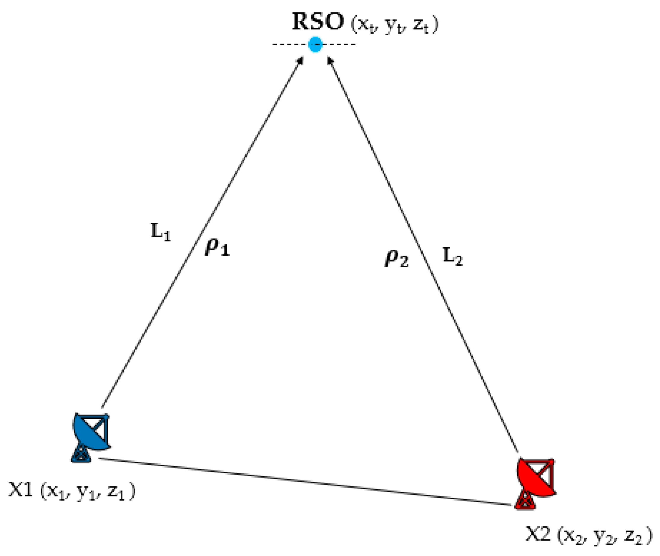
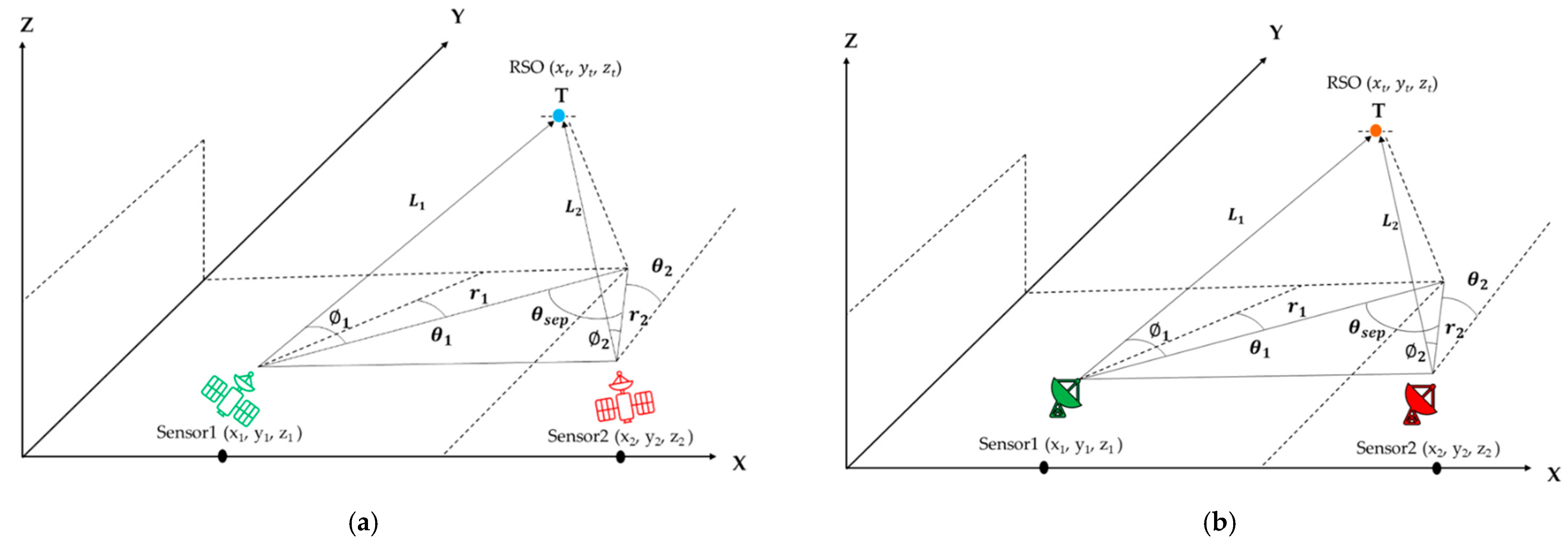
2.1. Triangulation Problem
2.2. Tracking Algorithm
- (xt,yt,zt) = target RSO position coordinates,
- (xi,yi,zi) = corresponding sensor position coordinates
- ri = horizontal ranges from the x − y components of the corresponding sensor to the x and y components of the RSO,
- φi = corresponding sensor to RSO elevation angle,
- θi = corresponding sensor to RSO azimuth angle.
- i = 1, 2 (number of sensors used to perform triangulation)
2.3. Uncertainty Quantification
2.4. Covariance Matrix to Ellipsoid
- is a vector in the Cartesian coordinates about the nominal position (origin), of the ellipsoid.
- R = rotation matrix,
- A = diagonal eigenvalues matrix respectively, which are derived from Q.
3. Trajectory Optimization Techniques Overview
- The necessary conditions, including the co-state differential equations, the Hamiltonian, and the optimality conditions, must be expressed analytically.
- Due to discretization of co-states, the problem size becomes large.
- The analyst must guess certain aspects of the solution, such as portions of the time domain containing constrained or unconstrained control arcs.
- The domain of convergence decreases due to the requirement of the initial guess being close to optimal solution.
4. Case Studies
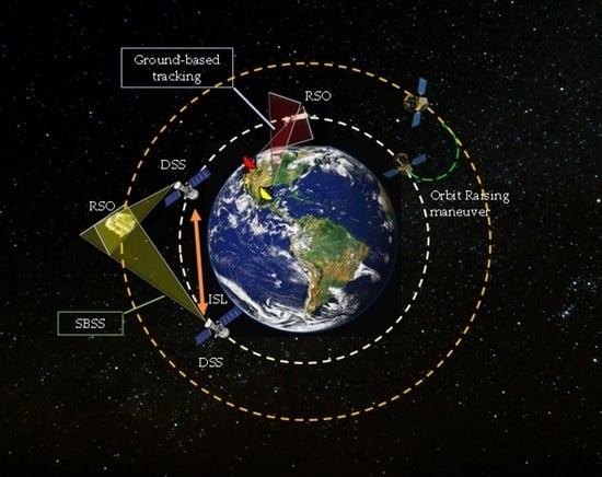
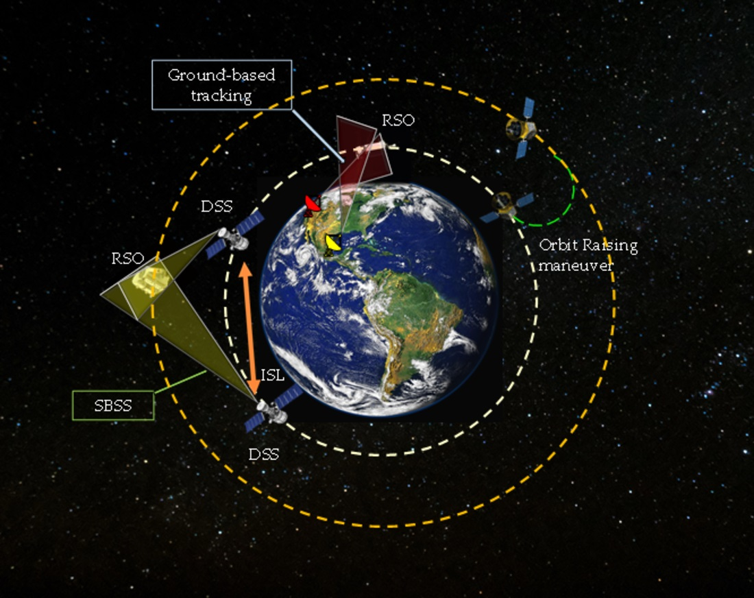
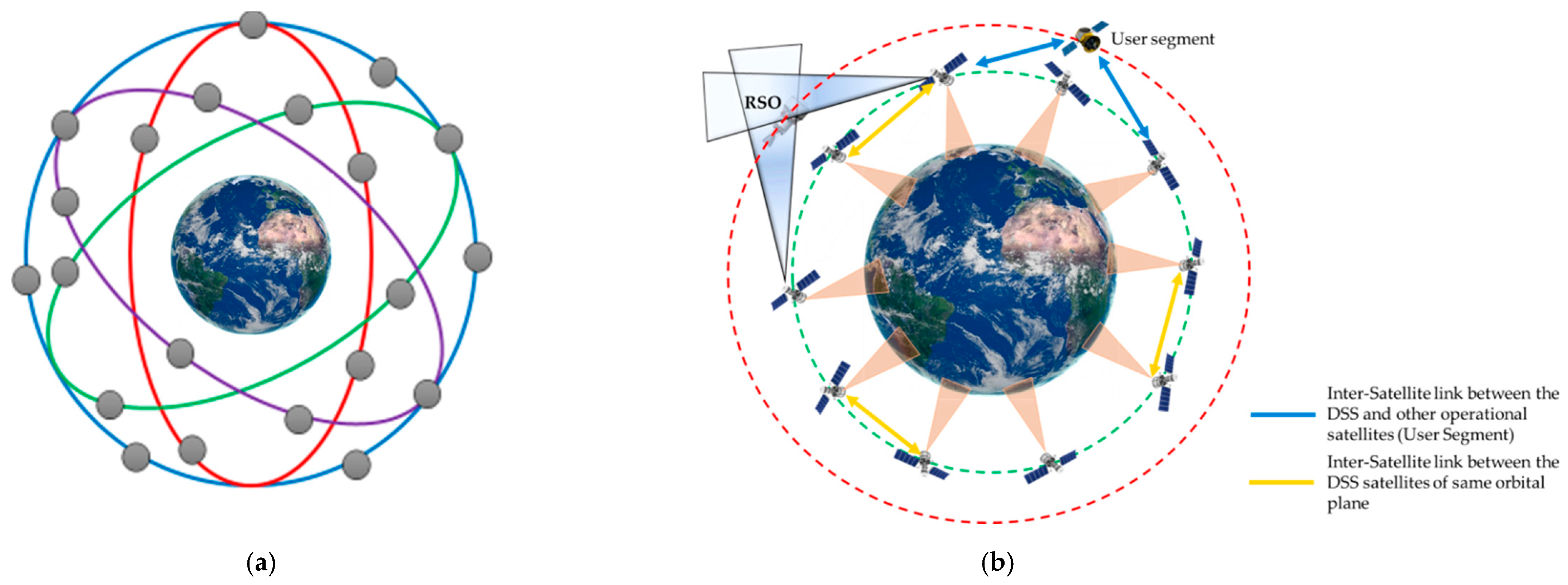
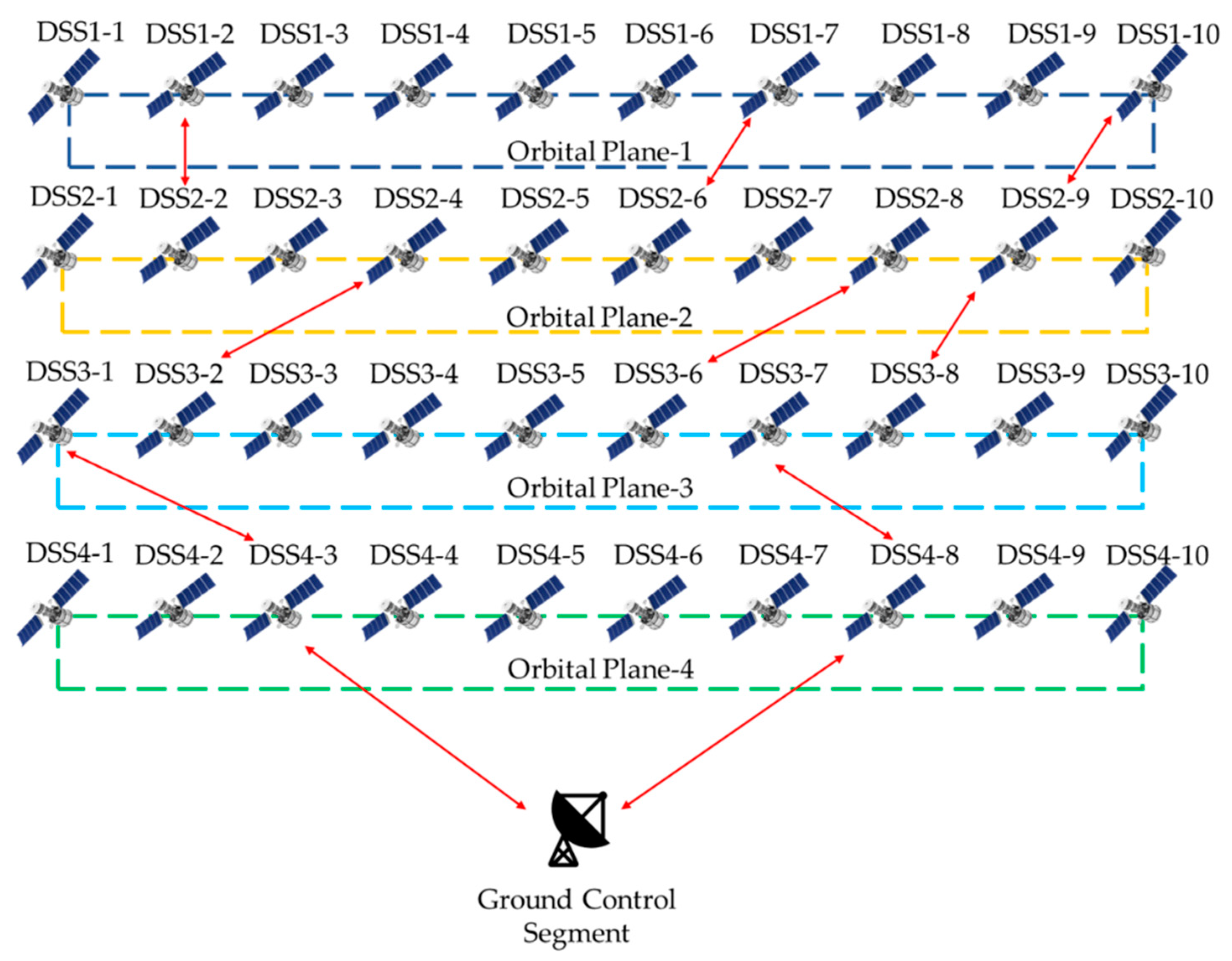
4.1. SBSS Scenario
- The system configuration must be feasible for multiple applications. For instance, AN for CA (current interest), SBSS for STM, multi-domain traffic management (MDTM) [88], and point-to-point sub orbital space transport, which are envisioned in the longer term.
- The satellites in the DSS architecture should complement each other and form ad-hoc or optional teams to make autonomous decisions and maximize mission objectives without involving the ground control segment, making them distinct compared to conventional satellite systems.
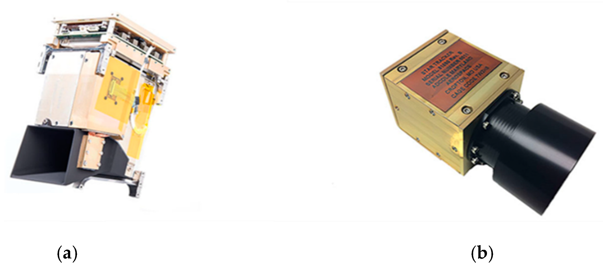
- The star trackers on board track the RSOs with the stars in the background.
- The participating spacecraft are equipped with state-of-the-art GPS for positioning and navigation that provide a full set of navigation data.
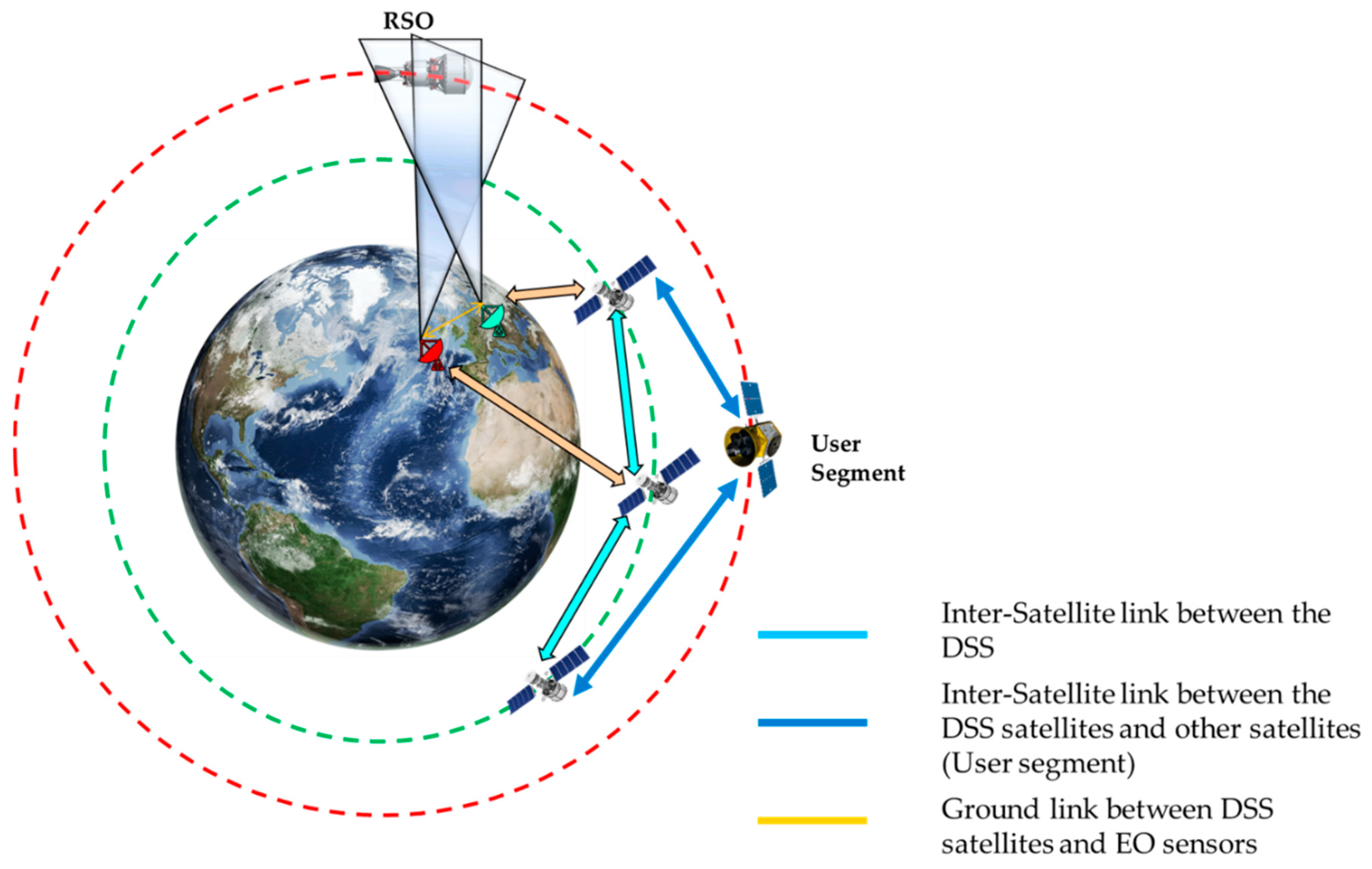
- The RSO position is estimated by simultaneous optical measurements obtained from two different spacecraft.
- The participating spacecraft share their position information and the estimated RSO position through a network.
- Mutual separation between the spacecraft belonging to the DSS constellation is guaranteed using intersatellite links and continuous monitoring from the ground stations.
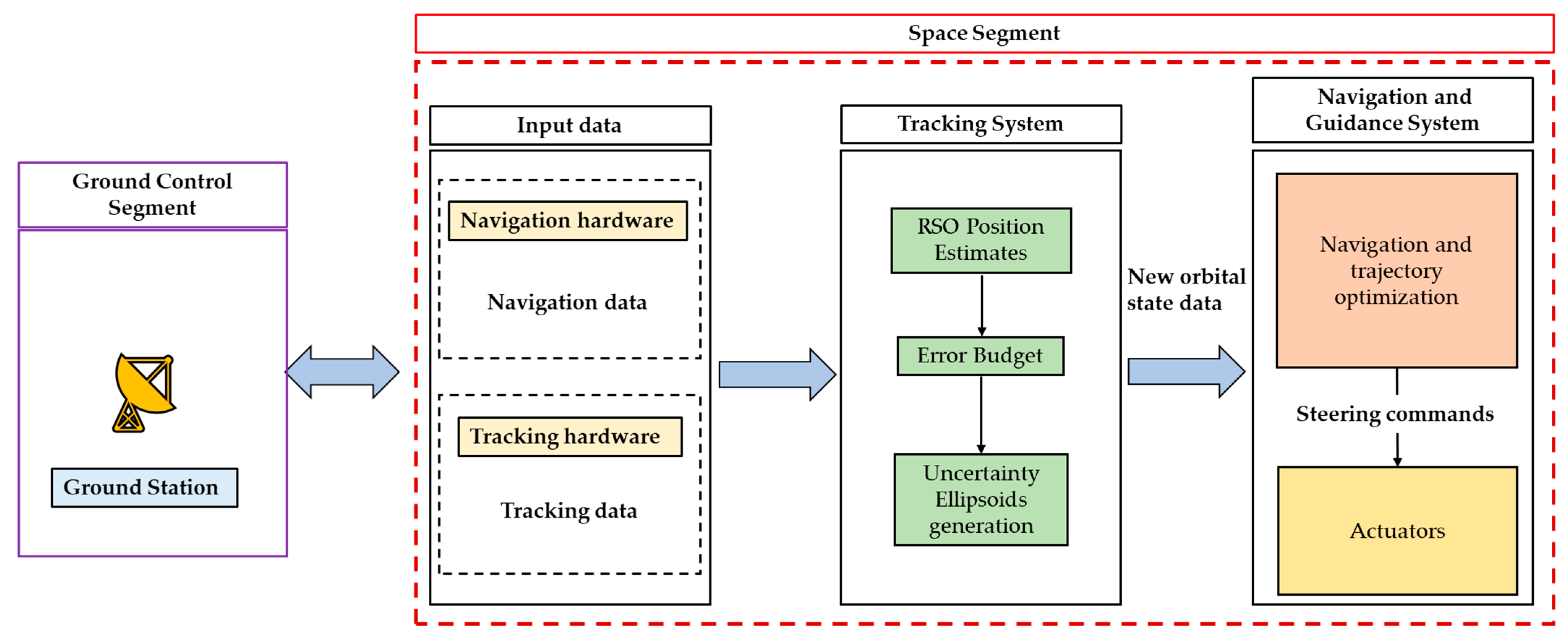
- Navigation hardware comprises the state-of-the-art GPS to obtain a full set of navigation data comprising the DSS satellite positions, velocities, and attitude rates.
- Tracking hardware comprises star trackers that track the RSO.
- The obtained data from the hardware is used as inputs by the on-board Tracking System to obtain the RSO position estimates, error measurement budget, and to generate the uncertainty ellipsoids.
- The navigation and guidance system exploits the data generated by the tracking system for trajectory optimization and AN/manoeuvring to generate the steering commands.
- Actuators use the steering commands to perform the collision avoidance manoeuvres in order to avoid a collision with the RSO.
4.2. Case Study 2—Ground-Based Surveillance
- The DSS assets are placed in a nearly circular low earth orbit (LEO) at an altitude of 500 km to carry out Earth observation activities.
- The participating spacecraft are equipped with sophisticated GPS for positioning and navigation that provide a full set of navigation data.
- The estimated RSO position from ground-based sensors is uplinked to the DSS assets to ensure their safety.
- The participating spacecraft share their position information and the RSO position estimates with other satellites using inter-satellite links (ISL).
- The ground-based EO sensors assumed in this scenario are similar to the sensors used in [93] and operate in the infra-red (IR) region between the wavelengths of 3–12 µm.
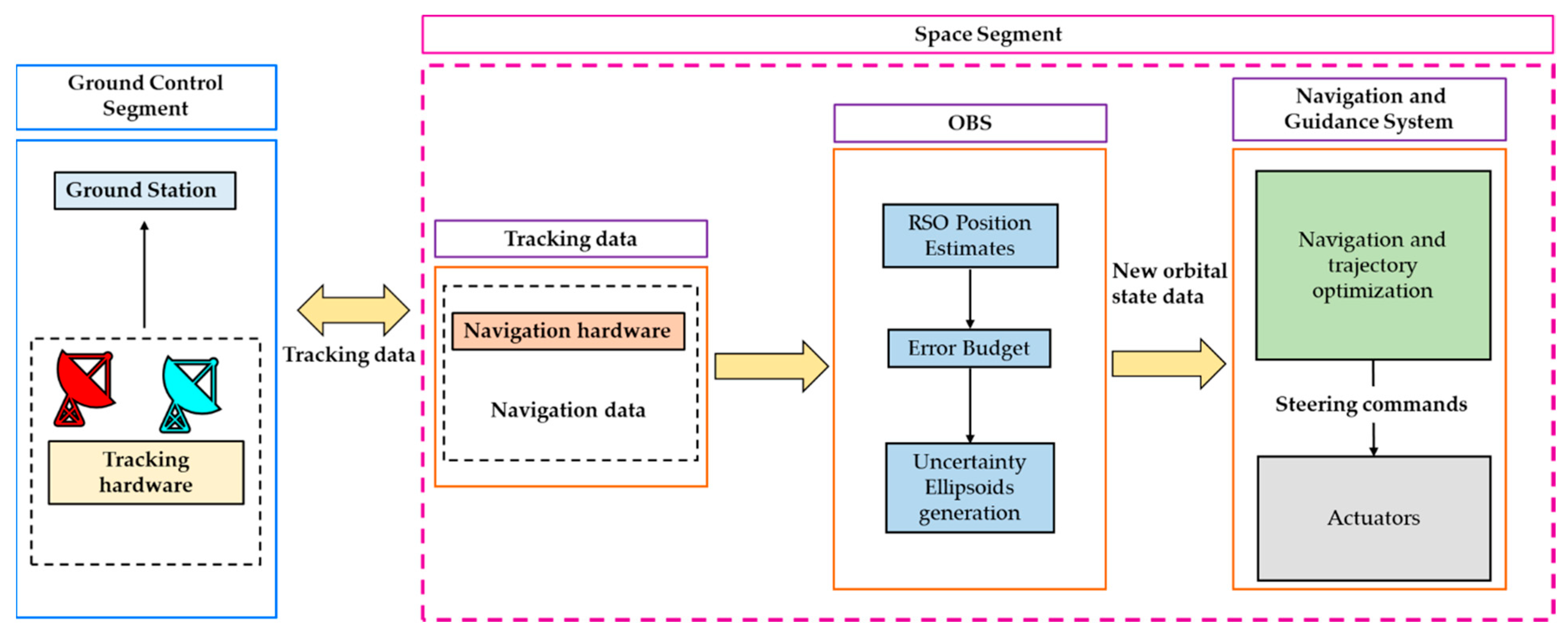
- Navigation hardware comprises the state of the art GPS to obtain a full set of navigation data comprising the DSS satellite positions, velocities, and attitude rates.
- Tracking hardware comprises ground-based EO sensors that track the RSO by simultaneous optical measurements.
- The obtained data from the hardware are used as inputs by the On-Board System (OBS) to obtain the RSO position estimates, error measurement budget, and to generate the uncertainty ellipsoids.
- The navigation and guidance system exploits the data generated by the OBS for trajectory planning and optimization to generate the steering commands.
- Actuators use the steering commands to perform the collision avoidance manoeuvres in order to avoid a collision with the RSO.
5. Results and Discussions
- rt = the position vector of the RSO in ECI frame,
- fi = orbital perturbations that take into account J2 perturbations and drag.
- The velocity of the RSO can be calculated by integrating Equation (60).
5.1. Space-Based Tracking Scenario
5.2. Ground-Based Tracking Scenario
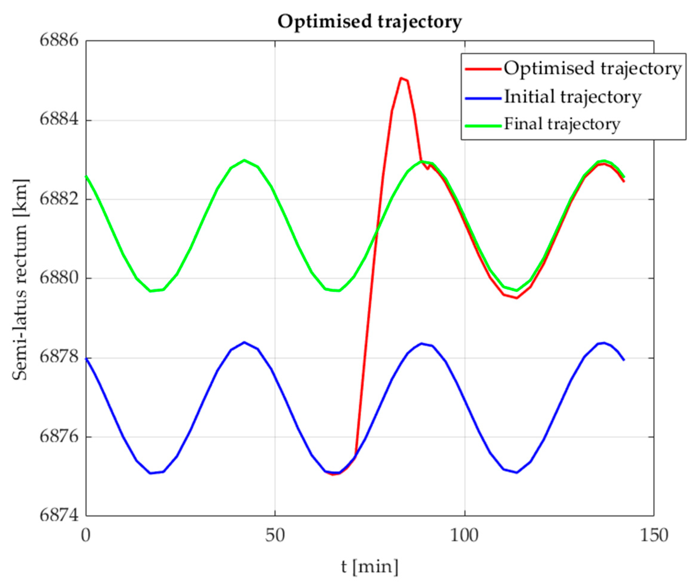
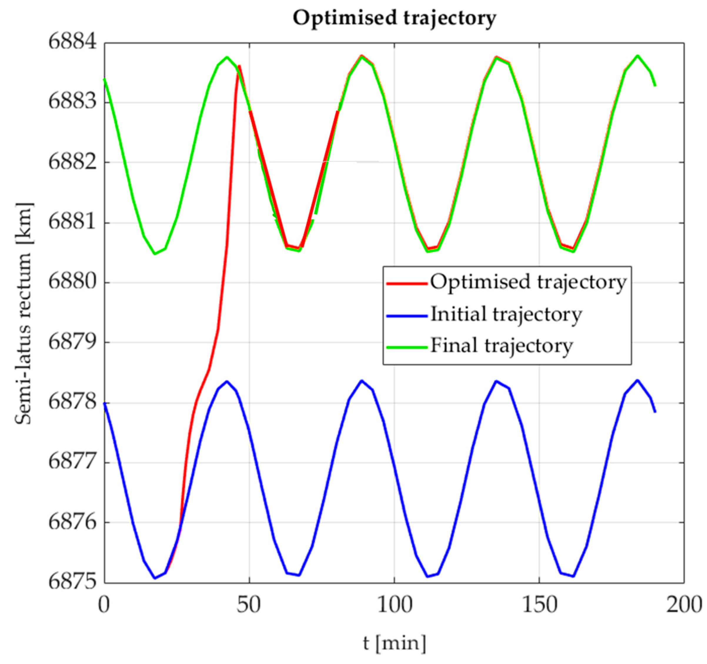
5.3. Trajectory Optimization for Collision Avoidance
6. Conclusions and Future Work
Author Contributions
Funding
Conflicts of Interest
References
- Space Environment Statistics Space Debris User Portal. Available online: https://sdup.esoc.esa.int/discosweb/statistics/ (accessed on 16 July 2022).
- Kessler, D.; Johnson, N.; Liou, J.-C.; Matney, M. The Kessler Syndrome: Implications to Future Space operations. Adv. Astronaut. Sci. 2010, 137, 2010. [Google Scholar]
- Hilton, S.; Sabatini, R.; Gardi, A.; Ogawa, H.; Teofilatto, P. Space traffic management: Towards safe and unsegregated space transport operations. Prog. Aerosp. Sci. 2019, 105, 98–125. [Google Scholar] [CrossRef]
- Ackermann, M.R.; Kiziah, R.; Zimmer, P.C.; McGraw, J.; Cox, D. A systematic examination of ground-based and space-based approaches to optical detection and tracking of satellites. In Proceedings of the 31st Space Symposium, Technical Track, Colorado Springs, CO, USA, 13–17 April 2015. [Google Scholar]
- Flohrer, T.; Krag, H.; Klinkrad, H.; Schildknecht, T. Feasibility of performing space surveillance tasks with a proposed space-based optical architecture. Adv. Space Res. 2011, 47, 1029–1042. [Google Scholar] [CrossRef]
- Utzmann, J.; Wagner, A. SBSS Demonstrator: A Space-Based Telescope for Space Surveillance and Tracking; International Astronautical Federation: Paris, France, 2015. [Google Scholar]
- Felicetti, L.; Emami, M.R. A multi-spacecraft formation approach to space debris surveillance. Acta Astronaut. 2016, 127, 491–504. [Google Scholar] [CrossRef]
- Vanwijck, X.; Flohrer, T. Possible contribution of space-based assets for space situational awareness. In Proceedings of the 59th International Astronautical Congress, Glasgow, Scotland, 29 September–3 October 2008; pp. 2466–2472. [Google Scholar]
- Utzmann, J.; Wagner, A.; Silha, J.; Schildknecht, T.; Willemsen, P.; Teston, F.; Flohrer, T. Space-Based Space Surveillance and Tracking Demonstrator: Mission and System Design; International Astronautical Federation: Paris, France; p. 7.
- Gruntman, M. Passive optical detection of submillimeter and millimeter size space debris in low Earth orbit. Acta Astronaut. 2014, 105, 156–170. [Google Scholar] [CrossRef]
- Sabatini, R.; Battipede, M.; Cairola, F. Innovative Techniques for Spacecraft Separation Assurance and Debris Collision Avoidance. Master’s Thesis, RMIT University, Melbourne, VIC, Australia, 2020. [Google Scholar]
- Yunpeng, H.; Kebo, L.; Yan’gang, L.; Lei, C. Review on strategies of space-based optical space situational awareness. J. Syst. Eng. Electron. 2021, 32, 1152–1166. [Google Scholar] [CrossRef]
- Gaposchkin, E.M.; von Braun, C.; Sharma, J. Space-Based Space Surveillance with the Space-Based Visible. J. Guid. Control Dyn. 2000, 23, 148–152. [Google Scholar] [CrossRef]
- Sharma, J. Space-Based Visible Space Surveillance Performance. J. Guid. Control Dyn. 2000, 23, 153–158. [Google Scholar] [CrossRef]
- Stokes, G.; Vo, C.; Sridharan, R.; Sharma, J. The space-based visible program. In Proceedings of the Space 2000 Conference and Exposition, Long Beach, CA, USA, 19–21 September 2000; p. 5334. [Google Scholar]
- Space Based Space Surveillance (SBSS). Available online: https://www.globalsecurity.org/space/systems/sbss.htm (accessed on 13 July 2022).
- Maskell, P.; Oram, L. Sapphire: Canada’s answer to space-based surveillance of orbital objects. In Proceedings of the Advanced Maui Optical and Space Surveillance Conference, Maui, HI, USA, 16–19 September 2008. [Google Scholar]
- Steve Wozniak and Alex Fielding’s Startup Privateer Aims to be the Google Maps of Space. TechCrunch. Available online: https://social.techcrunch.com/2021/10/12/steve-wozniak-privateer-space-company/ (accessed on 16 July 2022).
- Liu, M.; Wang, H.; Yi, H.; Xue, Y.; Wen, D.; Wang, F.; Shen, Y.; Pan, Y. Space Debris Detection and Positioning Technology Based on Multiple Star Trackers. Appl. Sci. 2022, 12, 3593. [Google Scholar] [CrossRef]
- Hussain, K.F.; Thangavel, K.; Gardi, A.; Sabatini, R. Autonomous Optical Sensing for Space-Based Space Surveillance. Presented at the IEEE Aerospace conference, Big Sky, MT, USA, 23. In Proceedings of the Presented at the IEEE Aerospace Conference, Big Sky, MT, USA, March 2023. [Google Scholar]
- Araguz, C.; Bou-Balust, E.; Alarcón, E. Applying autonomy to distributed satellite systems: Trends, challenges, and future prospects. Syst. Eng. 2018, 21, 401–416. [Google Scholar] [CrossRef]
- Le Moigne, J.; Adams, J.C.; Nag, S. A New Taxonomy for Distributed Spacecraft Missions. IEEE J. Sel. Top. Appl. Earth Obs. Remote Sens. 2020, 13, 872–883. [Google Scholar] [CrossRef]
- Brown, O.; Eremenko, P. The Value Proposition for Fractionated Space Architectures. In Space 2006; American Institute of Aeronautics and Astronautics: Reston, VA, USA, 2006. [Google Scholar] [CrossRef]
- Hussain, K.; Hussain, K.; Carletta, S.; Teofilatto, P. Deployment of a microsatellite constellation around the Moon using chaotic multi body dynamics. In Proceedings of the 71st International Astronautical Congress (IAC), Dubai, United Arab Emirates, 25–29 October 2021. [Google Scholar]
- Golkar, A.; Cruz, I.L.I. The Federated Satellite Systems paradigm: Concept and business case evaluation. Acta Astronaut. 2015, 111, 230–248. [Google Scholar] [CrossRef]
- Graziano, M.D. Overview of Distributed Missions. In Distributed Space Missions for Earth System Monitoring; D’Errico, M., Ed.; Springer: New York, NY, USA, 2013; pp. 375–386. [Google Scholar] [CrossRef]
- von Maurich, O.; Golkar, A. Data authentication, integrity and confidentiality mechanisms for federated satellite systems. Acta Astronaut. 2018, 149, 61–76. [Google Scholar] [CrossRef]
- Ben-Larbi, M.K.; Pozo, K.F.; Haylok, T.; Choi, M.; Grzesik, B.; Haas, A.; Krupke, D.; Konstanski, H.; Schaus, V.; Fekete, S.P.; et al. Towards the automated operations of large distributed satellite systems. Part 1: Review and paradigm shifts. Adv. Space Res. 2021, 67, 3598–3619. [Google Scholar] [CrossRef]
- Selva, D.; Golkar, A.; Korobova, O.; Cruz, I.L.I.; Collopy, P.; de Weck, O.L. Distributed Earth Satellite Systems: What Is Needed to Move Forward? J. Aerosp. Inf. Syst. 2017, 14, 412–438. [Google Scholar] [CrossRef]
- Yaglioglu, B. A fractionated spacecraft architecture for Earth observation missions. Master’s Thesis, Luleå University of Technology, Luleå, Sweden, 2011. [Google Scholar]
- Stephens, G.L.; Vane, D.G.; Boain, R.J.; Mace, G.G.; Sassen, K.; Wang, Z.; Illingworth, A.J.; O’connor, E.J.; Rossow, W.B.; Durden, S.L.; et al. The CloudSat mission and the A-Train: A new dimension of space-based observations of clouds and precipitation. Bull. Am. Meteorol. Soc. 2002, 83, 1771–1790. [Google Scholar] [CrossRef]
- Cluster—Satellite Missions—eoPortal Directory. Available online: https://directory.eoportal.org/web/eoportal/satellite-missions/content/-/article/cluster (accessed on 16 July 2022).
- Fang, W.; An, Y.; He, K.; Li, J.; Wang, B.; Li, J.; Wang, Q.; Guo, Q. Energy-Efficient Network Transmission between Satellite Swarms and Earth Stations Based on Lyapunov Optimization Techniques. Math. Probl. Eng. 2014, 2014, 1–10. [Google Scholar] [CrossRef]
- Golkar, A. Federated satellite systems (FSS): A vision towards an innovation in space systems design. In Proceedings of the IAA Symposium on Small Satellites for Earth Observation, Berlin, Germany, 6–10 May 2013. [Google Scholar]
- Poghosyana, A.; Llucha, I.; Matevosyana, H.; Lamba, A.; Morenoa, C.A.; Taylora, C.; Golkara, A.; Coteb, J.; Mathieub, S.; Pierottib, S.; et al. Unified classification for distributed satellite systems. In Proceedings of the 4th International Federated and Fractionated Satellite Systems Workshop, Rome, Italy, 10 October 2016. [Google Scholar]
- Hilton, S.; Gardi, A.; Sabatini, R.; Ezer, N.; Desai, S. Human-Machine System Design for Autonomous Distributed Satellite Operations. In Proceedings of the 2020 AIAA/IEEE 39th Digital Avionics Systems Conference (DASC), San Antonio, TX, USA, 1–8 October 2020. [Google Scholar] [CrossRef]
- Hilton, S.; Cairola, F.; Gardi, A.; Sabatini, R.; Pongsakornsathien, N.; Ezer, N. Uncertainty quantification for space situational awareness and traffic management. Sensors 2019, 19, 4361. [Google Scholar] [CrossRef]
- Sanders-Reed, J.N. Vehicle real-time attitude-estimation system (VRAES). In Acquisition, Tracking, and Pointing X.; SPIE: Bellingham, WA, USA, 1996; Volume 2739, pp. 266–277. [Google Scholar] [CrossRef]
- Walton, J.S. Image-based motion measurement: New technology, new applications. In Proceedings of the 21st International Congress on: High-Speed Photography and Photonics, Taejon, Republic of Korea, 30 May 1995; Volume 2513, pp. 862–880. [Google Scholar] [CrossRef]
- Guezennec, Y.G.; Brodkey, R.S.; Trigui, N.; Kent, J.C. Algorithms for fully automated three-dimensional particle tracking velocimetry. Exp. Fluids 1994, 17, 209–219. [Google Scholar] [CrossRef]
- Adamczyk, A.A.; Rimai, L. Reconstruction of a 3-dimensional flow field from orthogonal views of seed track video images. Exp. Fluids 1988, 6, 380–386. [Google Scholar] [CrossRef]
- Yanagisawa, T.; Kurosaki, H.; Oda, H.; Tagawa, M. Ground-based optical observation system for LEO objects. Adv. Space Res. 2015, 56, 414–420. [Google Scholar] [CrossRef]
- Chen, L.; Liu, C.; Li, Z.; Kang, Z. A New Triangulation Algorithm for Positioning Space Debris. Remote Sens. 2021, 13, 4878. [Google Scholar] [CrossRef]
- Lloyd, K.H. Concise Method for Photogrammetry of Objects in the Sky; Weapons Research Establishment: Salisbury, Australia, 1971. [Google Scholar]
- Powers, J.W. Range Trilateration Error Analysis; IEEE: Piscataway, NJ, USA, 1966; pp. 572–585. [Google Scholar] [CrossRef]
- Long, S.A.T. Analytical Expressions for Position Error in Triangulation Solution of Point in Space for Several Station Configurations. L–9235, June 1974. Available online: https://ntrs.nasa.gov/citations/19740020173 (accessed on 18 July 2022).
- Sanders-Reed, J.N. Impact of tracking system knowledge on multisensor 3D triangulation. In Acquisition, Tracking, and Pointing XVI.; SPIE: Bellingham, WA, USA, 2002; Volume 4714, pp. 33–41. [Google Scholar]
- Sanders-Reed, J.N. Error propagation in two-sensor three-dimensional position estimation. Opt. Eng. 2001, 40, 627–636. [Google Scholar] [CrossRef]
- Sanders-Reed, J.N. Triangulation Position Error Analysis for Closely Spaced Imagers; SAE International: Warrendale, PA, USA. [CrossRef]
- Hauschild, A.; Markgraf, M.; Montenbruck, O. GPS receiver performance on board a LEO satellite. Gnss 2014, 9, 47–57. [Google Scholar]
- Curry, G.R. Radar System Performance Modeling, Artech House; Inc. Ed.: Norwood, MA, USA, 2005. [Google Scholar]
- Vallado, D.A. Fundamentals of Astrodynamics and Applications; Springer Science & Business Media: Berlin/Heidelberg, Germany, 2001. [Google Scholar]
- Wijewickrema, S.N.; Papliński, A.P. Principal component analysis for the approximation of an image as an ellipse. In Proceedings of the 13th International Conference in Central Europe on Computer Graphics, Visualization and Computer Vision, Plzen, Czech Republic, 31 January–4 March 2005. [Google Scholar]
- Behdinan, K.; Perez, R.E.; Liu, H.T. Multidisciplinary design optimization of aerospace systems. In Proceedings of the Canadian Design Engineering Network (CDEN) Conference, Kaninaskis, AB, USA, 18–20 July 2005. [Google Scholar] [CrossRef]
- Carrington, C.K.; Junkins, J.L. Optimal nonlinear feedback control for spacecraft attitude maneuvers. J. Guid. Control Dyn. 1986, 9, 99–107. [Google Scholar] [CrossRef]
- Bilimoria, K.D.; Wie, B. Time-optimal three-axis reorientation of a rigid spacecraft. J. Guid. Control Dyn. 1993, 16, 446–452. [Google Scholar] [CrossRef]
- Betts, J.T. Survey of Numerical Methods for Trajectory Optimization. J. Guid. Control Dyn. 1998, 21, 193–207. [Google Scholar] [CrossRef]
- Polovinkin, E.S. Pontryagin’s Direct Method for Optimization Problems with Differential Inclusion. In Proceedings of the Steklov Institute of Mathematics; Pleiades Publishing, Ltd.: Moscow, Russia, 2019; Volume 304, pp. 241–256. [Google Scholar] [CrossRef]
- Ben-Asher, J.Z. Optimal Control Theory with Aerospace Applications; The American Institute of Aeronautics and Astronautics: Reston, VA, USA, 2010. [Google Scholar]
- Conway, B.A. Spacecraft Trajectory Optimization; Cambridge University Press: Cambridge, UK, 2010. [Google Scholar]
- Gondelach, D.J.; Noomen, R. Hodographic-Shaping Method for Low-Thrust Interplanetary Trajectory Design. J. Spacecr. Rockets 2015, 52, 728–738. [Google Scholar] [CrossRef]
- Vasile, M.; De Pascale, P.; Casotto, S. On the optimality of a shape-based approach based on pseudo-equinoctial elements. Acta Astronaut. 2007, 61, 286–297. [Google Scholar] [CrossRef]
- Taheri, E.; Abdelkhalik, O. Initial three-dimensional low-thrust trajectory design. Adv. Space Res. 2016, 57, 889–903. [Google Scholar] [CrossRef]
- Taheri, E.; Abdelkhalik, O. Shape Based Approximation of Constrained Low-Thrust Space Trajectories using Fourier Series. J. Spacecr. Rockets 2012, 49, 535–546. [Google Scholar] [CrossRef]
- Shirazi, A.; Ceberio, J.; Lozano, J.A. Spacecraft trajectory optimization: A review of models, objectives, approaches and solutions. Prog. Aerosp. Sci. 2018, 102, 76–98. [Google Scholar] [CrossRef]
- Voß, S.; Martello, S.; Osman, I.H.; Roucairol, C. (Eds.) Meta-Heuristics: Advances and Trends in Local Search Paradigms for Optimization; Springer: Boston, MA, USA, 1998. [Google Scholar] [CrossRef]
- Câmara, D. 4—Swarm Intelligence (SI). In Bio-Inspired Networking; Câmara, D., Ed.; Elsevier: Amsterdam, The Netherlands, 2015; pp. 81–102. [Google Scholar] [CrossRef]
- Blum, C.; Roli, A. Metaheuristics in combinatorial optimization: Overview and conceptual comparison. ACM Comput. Surv. CSUR 2003, 35, 268–308. [Google Scholar] [CrossRef]
- Xiong, N.; Molina, D.; Leon, M.; Herrera, F. A Walk into Metaheuristics for Engineering Optimization: Principles, Methods and Recent Trends. Int. J. Comput. Intell. Syst. 2015, 8, 606–636. [Google Scholar] [CrossRef]
- Leboucher, C.; Shin, H.-S.; Siarry, P.; Le Ménec, S.; Chelouah, R.; Tsourdos, A. Convergence proof of an enhanced Particle Swarm Optimisation method integrated with Evolutionary Game Theory. Inf. Sci. 2016, 346, 389–411. [Google Scholar] [CrossRef]
- Kennedy, J.; Eberhart, R. Particle swarm optimization. In Proceedings of ICNN’95—International Conference on Neural Networks; IEEE: Piscataway, NJ, USA, 1995; Volume 4, pp. 1942–1948. [Google Scholar] [CrossRef]
- Lin, M.; Zhang, Z.-H.; Zhou, H.; Shui, Y. Multiconstrained Ascent Trajectory Optimization Using an Improved Particle Swarm Optimization Method. Int. J. Aerosp. Eng. 2021, 2021, 1–12. [Google Scholar] [CrossRef]
- Rahimi, A.; Kumar, K.D.; Alighanbari, H. Particle Swarm Optimization Applied to Spacecraft Reentry Trajectory. J. Guid. Control Dyn. 2013, 36, 307–310. [Google Scholar] [CrossRef]
- Huang, P.; Xu, Y. PSO-Based Time-Optimal Trajectory Planning for Space Robot with Dynamic Constraints. In Proceedings of the 2006 IEEE International Conference on Robotics and Biomimetics, Kunming, China, 17–20 December 2006; IEEE: Piscataway, NJ, USA, 2006; pp. 1402–1407. [Google Scholar] [CrossRef]
- Betts, J.T. Practical Methods for Optimal Control and Estimation Using Nonlinear Programming, 2nd ed.; Society for Industrial and Applied Mathematics: Philadelphia, PA, USA, 2010. [Google Scholar] [CrossRef]
- Baù, G.; Hernando-Ayuso, J.; Bombardelli, C. A generalization of the equinoctial orbital elements. Celest. Mech. Dyn. Astron. 2021, 133, 1–29. [Google Scholar] [CrossRef]
- Stuart, E. Applied Nonsingular Astrodynamics: Optimal Low-Thrust Orbit Transfer JA Kéchichian Cambridge University Press, University Printing House, Shaftesbury Road, Cambridge CB2 8BS, UK. 2018. xvii; 461 pp. Illustrated.£ 89.99. ISBN 978-1-108-47236-4. Aeronaut. J. 2020, 124, 2036–2037. [Google Scholar]
- Rajendra, P.P.; Kuga, H.K. An evaluation of Jacchia and MSIS 90 atmospheric models with CBERS data. Acta Astronaut. 2001, 48, 579–588. [Google Scholar] [CrossRef]
- Climate change—The Official Portal of the UAE Government. Available online: https://u.ae/en/information-and-services/environment-and-energy/climate-change/climate-change (accessed on 24 December 2022).
- Thangavel, K.; Spiller, D.; Sabatini, R.; Marzocca, P. On-board Data Processing of Earth Observation Data Using 1-D CNN. In Proceedings of the SmartSat CRC Conference 2022, Sydney, Australia, 12–13 September 2022. [Google Scholar] [CrossRef]
- Thangavel, K.; Spiller, D.; Sabatini, R.; Marzocca, P.; Esposito, M. Near Real-time Wildfire Management Using Distributed Satellite System. IEEE Geosci. Remote Sens. Lett. 2022, 20, 1–5. [Google Scholar] [CrossRef]
- Thangavel, K.; Spiller, D.; Sabatini, R.; Amici, S.; Sasidharan, S.T.; Fayek, H.; Marzocca, P. Autonomous Satellite Wildfire Detection Using Hyperspectral Imagery and Neural Networks: A Case Study on Australian Wildfire. Remote Sens. 2023, 15, 720. [Google Scholar] [CrossRef]
- Spiller, D.; Thangavel, K.; Sasidharan, S.T.; Amici, S.; Ansalone, L.; Sabatini, R. Wildfire segmentation analysis from edge computing for on-board real-time alerts using hyperspectral imagery. In Proceedings of the 2022 IEEE International Conference on Metrology for Extended Reality, Artificial Intelligence and Neural Engineering (MetroXRAINE), Rome, Italy, 25–27 October 2022; pp. 725–730. [Google Scholar] [CrossRef]
- Thangavel, K.; Servidia, P.; Sabatini, R.; Marzocca, P.; Fayek, H.; Spiller, D. Distributed Satellite System for Maritime Domain Awareness. In Proceedings of the 20th Australian International Aerospace Congress (AIAC20), Melbourne, VIC, Australia, 27–28 February 2023. [Google Scholar]
- Ettouati, I.; Mortari, D.; Pollock, T. Space surveillance using star trackers. Part I: Simulations. Pap. AAS 2006, 06-231. [Google Scholar]
- Lagona, E.; Hilton, S.; Afful, A.; Gardi, A.; Sabatini, R. Autonomous Trajectory Optimisation for Intelligent Satellite Systems and Space Traffic Management. Acta Astronaut. 2022, 194, 185–201. [Google Scholar] [CrossRef]
- Flohrer, T.; Peltonen, J.; Kramer, A.; Eronen, T.; Kuusela, J.; Riihonen, E.; Schildknecht, T.; Stöveken, E.; Valtonen, E.; Wokke, F.; et al. Space-Based Optical Observations of Space Debris. In Proceedings of the 4th European Conference on Space Debris, Darmstadt, Germany, 18–20 April 2005; p. 165. [Google Scholar]
- Thangavela, K.; Gardia, A.; Hiltona, S.; Affula, A.M.; Sabatinib, R. Towards Multi-Domain Traffic Management. Structure 2021, 1, 2. [Google Scholar]
- HyperScout-2|InCubed. Available online: https://incubed.esa.int/portfolio/hyperscout-2/ (accessed on 24 December 2022).
- MAI-SS—Star Tracker|SatCatalog. Available online: https://www.satcatalog.com/component/mai-ss/ (accessed on 25 December 2022).
- Thangavel, K.; Spiller, D.; Sabatini, R.; Servidia, P.; Marzocca, P.; Fayek, H.; Hussain, K.; Gardi, A. Trusted Autonomous Distributed Satellite System Operations for Earth Observation. In Proceedings of the 17th International Conference on Space Operations, Dubai, United Arab Emirates, 6–10 March 2023. [Google Scholar] [CrossRef]
- Hussain, K.F.; Thangavel, K.; Gardi, A.; Sabatini, R. Autonomous tracking of Resident Space Objects using multiple ground-based Electro-Optical sensors. In Proceedings of the 17th International Conference on Space Operations, Dubai, United Arab Emirates, 6–10 March 2023. [Google Scholar]
- Infrared Detectors for Space Application. Vigo USA. Available online: https://vigophotonics.com/us/applications/infrared-detectors-for-space-application/ (accessed on 31 January 2023).
- Zhai, G.; Zhang, J.; Zhou, Z. On-orbit target tracking and inspection by satellite formation. J. Syst. Eng. Electron. 2013, 24, 879–888. [Google Scholar] [CrossRef]
- CubeSat Propulsion System EPSS, NanoAvionics. Available online: https://nanoavionics.com/cubesat-components/cubesat-propulsion-system-epss/ (accessed 2 January 2023).


| USA | Russia | Japan | Europe | ||||
|---|---|---|---|---|---|---|---|
| System | Year | System | Year | System | Year | System | Year |
| Thule radar | 1943 | Dnepr radar | 1963 | BSGC | 2002 | GRAVES (France) | 2005 |
| Eglin radar | 1969 | Dunay-3U radar | 1968 | KSGC | 2004 | TIRA (Germany) | 2009 |
| GEODSS | 1980 | Daryal radar | 1984 | ||||
| SST | 2011 | Don-2N radar | 1996 | ||||
| Space fence | 2020 | Okno optical complex | 1997 | ||||
| Krona system | 2008 | ||||||
| Payload | HyperScout-2 |
|---|---|
| Field Of View (FOV) | channel 1: 31° × 16° channel 2: 31° × 16° |
| Ground Sample Distance (GSD) | channel 1: 75 m channel 2: 490 m |
| Swath | 310 × 150 km |
| Active Pixels | channel 1: 4000 × 1850 px channel 2: 1024 × 768 px |
| Spectral Range | channel 1: 400–1000 nm channel 2: 8000–14,000 nm |
| Spectral Bands | channel 1: 45 channel 2: 3 |
| Spectral Resolution | channel 1: 16 nm channel 2: 1100 nm (B1, B2) and 6000 nm (B3) |
| Signal to Noise Ratio (SNR) | channel 1: 50–100 channel 2: 0.5–3000 |
| Power | 12 W |
| Performance Parameter | Specification |
|---|---|
| Accuracy (Cross Axis/Boresight) | 5.7 arcsec/27 arcsec |
| Acquisition Time | 130 ms Acq, 105 ms Track (typical) |
| Max Tracking Rate | >2.0°/s |
| Update Rate | 4 Hz |
| Lens | 0.9in f1.2 BK7 Glass |
| Orbital Parameters | Sensor 1 | Sensor 2 | Cartesian Coordinates | Sensor 1 | Sensor 2 |
|---|---|---|---|---|---|
| a (km) | 6878 | 6878 | Xi (km) | 6456.74 | 3843.01 |
| e | 0.001 | 0.001 | Yi (km) | −367.63 | −891.28 |
| i (deg) | 99 | 99 | Zi (km) | 2321.12 | 5627.35 |
| ω (deg) | 20 | 20 | VX (km/s) | −2.6 | −6.31 |
| Ω (deg) | 0 | 0 | VY (km/s) | −1.12 | −0.66 |
| θ (deg) | 0 | 36 | VZ (km/s) | 7.07 | 4.21 |
| Cartesian Coordinate | xt (km) | yt (km) | zt (km) | R (km) |
|---|---|---|---|---|
| RSO-state parameters | 5397.7 | −2446 | 7908.3 | 2265.65 |
| Total Error (σ’s) | 4.7 | 10.46 | 20.36 | 9.12 |
| Cartesian Co-Ordinates | Xi (km) | Yi (km) | Zi (km) |
|---|---|---|---|
| Sensor 1 | 1880.82 | 13.78 | 6221.92 |
| Sensor 2 | −1502.52 | −5.24 | 6356.15 |
| Cartesian Co-Ordinates | R (km) | |||
|---|---|---|---|---|
| RSO-state parameters | 732.38 | −2240.1 | 11,285 | 2818.1 |
| Total Error (σ’s) | 5.4 | 7.6 | 21.55 | 7.78 |
| a (km) | e | i (deg) | ω (deg) | Ω (deg) | |
|---|---|---|---|---|---|
| 6878 | 0.001 | 99 | 20 | 360 | |
| 6882.7 | 0.001 | 99 | 20 | 360 | |
| 6883.4 | 0.001 | 99 | 20 | 360 |
| Tracking Scenario | tf (min) | αM (deg) | βM (deg) | fT | kT (rad) | p1 | p2 |
|---|---|---|---|---|---|---|---|
| Space-based | 28.97 | 3.02 | −2.62 | 0.5 | 0.178 | 0.93 | 9.96 |
| Ground-based | 30.75 | −1.44 | −3.05 | 0.09 | 0.258 | 1 | 7.55 |
Disclaimer/Publisher’s Note: The statements, opinions and data contained in all publications are solely those of the individual author(s) and contributor(s) and not of MDPI and/or the editor(s). MDPI and/or the editor(s) disclaim responsibility for any injury to people or property resulting from any ideas, methods, instructions or products referred to in the content. |
© 2023 by the authors. Licensee MDPI, Basel, Switzerland. This article is an open access article distributed under the terms and conditions of the Creative Commons Attribution (CC BY) license (https://creativecommons.org/licenses/by/4.0/).
Share and Cite
Hussain, K.F.; Thangavel, K.; Gardi, A.; Sabatini, R. Passive Electro-Optical Tracking of Resident Space Objects for Distributed Satellite Systems Autonomous Navigation. Remote Sens. 2023, 15, 1714. https://doi.org/10.3390/rs15061714
Hussain KF, Thangavel K, Gardi A, Sabatini R. Passive Electro-Optical Tracking of Resident Space Objects for Distributed Satellite Systems Autonomous Navigation. Remote Sensing. 2023; 15(6):1714. https://doi.org/10.3390/rs15061714
Chicago/Turabian StyleHussain, Khaja Faisal, Kathiravan Thangavel, Alessandro Gardi, and Roberto Sabatini. 2023. "Passive Electro-Optical Tracking of Resident Space Objects for Distributed Satellite Systems Autonomous Navigation" Remote Sensing 15, no. 6: 1714. https://doi.org/10.3390/rs15061714
APA StyleHussain, K. F., Thangavel, K., Gardi, A., & Sabatini, R. (2023). Passive Electro-Optical Tracking of Resident Space Objects for Distributed Satellite Systems Autonomous Navigation. Remote Sensing, 15(6), 1714. https://doi.org/10.3390/rs15061714