Determination of Bayesian Cramér–Rao Bounds for Estimating Uncertainties in the Bio-Optical Properties of the Water Column, the Seabed Depth and Composition in a Coastal Environment

Abstract

The monitoring of coastal areas using remote sensing techniques is an important issue to determine the bio-optical properties of the water column and the seabed composition. New hyperspectral satellite sensors (e.g., PRISMA, DESIS or EnMap) are developed to periodically observe ecosystems. The uncertainties in the retrieved geophysical products remain a key issue to release reliable data useful for the end-users. In this study, an analytical approach based on Information theory is proposed to investigate the Cramér–Rao lower Bounds (CRB) for the uncertainties in the ocean color parameters. Practically, during the inversion process, an a priori knowledge on the estimated parameters is used since their range of variation is supposed to be known. Here, a Bayesian approach is attempted to handle such a priori knowledge. A Bayesian CRB (BCRB) is derived using the Lee et al. semianalytical radiative transfer model dedicated to shallow waters. Both environmental noise and bio-optical parameters are supposed to be random vectors that follow a Gaussian distibution. The calculation of CRB and BCRB is carried out for two hyperspectral images acquired above the French mediterranean coast. The images were obtained from the recently launched hyperspectral sensors, namely the DESIS sensor (DLR Earth Sensing Imaging Spectrometer, German Aerospace Center), and PRISMA (Precursore IpperSpettrale della Mission Applicativa—ASI, Italian Space Adjency) sensor. The comparison between the usual CRB approach, the proposed BCRB approach and experimental errors obtained for the retrieved bathymetry shows the better ability of the BCRB to determine minimum error bounds.

1. Introduction

The degradation of coastal zone ecosystems requires large-scale precision monitoring. Optical remote sensing allows in-depth analysis of water quality and seabed composition [1,2,3,4,5]. The estimation of depth and bottom in optically shallow waters has important implications, e.g., for monitoring coral reefs [6,7], seagrass [8], invasive seaweed [9], or detecting changes in bathymetry [10,11].

The inherent optical properties (IOP) of the water column, i.e., the spectral absorption and backscattering coefficients, can be related to three optically active water constituents, which are Chlorophyll ($CHL$), Colored Dissolved Organic Matter ($CDOM$) and nonalgal Suspended Particulate Matter ($SPM$) [12]. Numerical models [13,14] and semianalytic models [15,16] have been developed to simulate the water attenuation as a function of the bathymetry, the bottom reflectance, the concentrations of chlorophyll ($C_{CHL}$), suspended matter ($C_{SPM}$), and colored dissolved organic matter absorption coefficient at 440 nm ($C_{CDOM}$) [17]. The inversion of the radiative transfer model that describes the propagation of light into the water column and its interaction with hydrosols and seabed allows the retrieval of the model parameters, $C_{CHL}$, $C_{SPM}$, $C_{CDOM}$, and in addition bathymetry in shallow waters [18]. If the bottom reflectance is not available, it can be approximated by a linear mixture of spectral signatures representative of the seabed, so the mixing coefficients should be estimated as well [19,20,21,22,23].

Hyperspectral imagery has shown to be more accurate instead of multispectral imagery for the decoupling of changes in bathymetry, water quality and seabed type [24,25,26,27,28,29,30,31,32,33]. Airborne hyperspectral sensors such as CASI [34], AVIRIS [35] or HYSPEX [36] are characterized by a high spatial resolution (1–2 m). Satellite sensors could cover larger areas than airborne sensors and a periodical revisit. However, there are few hypersectral sensors currently onboard satellite platforms. The DLR Earth Sensing Imaging Spectrometer (DESIS, 30 m), was launched in 2018 and integrated into the International Space Station (ISS) [37], the Precursore IpperSpettrale della Mission Applicativa—ASI (PRISMA, 30 m) was launched in 2019 [38], and the Environmental Mapping and Analysis Program (EnMap-DLR, 30 m) was launched in 2022. Finally, the BIODIVERSITY sensor, which is currently in preparation by CNES (french space agency) [39,40], will be characterized by a spatial resolution of 8 m. NASA’s Plankton, Aerosol, Clouds, ocean Ecosystem (PACE) satellite mission, which is scheduled in 2024, will carry the hyperspectral Ocean Color Instrument (OCI, 1 km spatial resolution) [41]. Recently, scientific publications related to the use of PRISMA and DESIS sensors in the acquatic environment showed the great interest of the community for using their up-to-date data for the remote sensing of aquatic ecosystem monitoring [42,43,44,45].

Accurate knowledge of uncertainties in the satellite derived geophysical products is particularly critical for remote sensing of dark targets such as those encountered in aquatic environments in comparison to terrestrial surfaces such as soil or vegetation. Because of the weak upward signal (the reflectance is typically less than $10\%$) exiting the water column, the spatial and spectral resolutions and the signal to noise ratio (SNR) should be carefully designed to properly acquire reliable hyperspectral measurements over aquatic systems. Associated uncertainties, which could be assessed in terms of root mean square error (RMSE) [46] or mean absolute difference [47], are informative on the confidence level of these products. Uncertainties are also required for designing future sensors [26,33], or for improving ocean model accuracy using data assimilation [48].

Uncertainties are often assessed by comparing the satellite-derived values with their ground truth measured values. In such case, uncertainties are related to sensor noise and radiometric specifications, as well as those induced by the inversion method, bio-optical modeling, atmospheric correction, and in situ measurements [46,47,49,50]. It should be noted that the uncertainty associated with the reflectance inversion to derive a given ocean colour parameter also depends on the actual value of the parameter. Many different statistical and physical methods have been developed for remote sensing of optically shallow waters [17,18,51,52,53,54,55,56,57,58]. The uncertainties established for a BIODIVERSITY-like sensor have been predicted using simulated images that matches the sensor features [40,59]. In [60,61], the authors present a method to obtain uncertainty estimates for inverted IOP by propagating the errors through the semianalytical model used for inversion. Most approaches require both remote-sensing data and ground truth to assess uncertainties. These approaches can be computationally expensive and also depend on the inversion method.

Cramér–Rao bounds ($CRB$) have been previously used to determine the performances of various sensors for a broad range of parameters [62,63,64]. The $CRB$ provides a lower bound on the variance of any unbiased estimator of a deterministic parameter [65,66,67,68]. In addition to fast computing time, the $CRB$ are convenient because they do not require hyperspectral data neither ground truth, and they are also independent of the method of inversion that is used to invert the water reflectance for deriving the bio-optical parameters of the water column. The $CRB$ theoretically provide the lower bounds for the uncertainty of the estimated parameters based on the probability law of the noise that corrupts the hyperspectral data and on the parametric radiative transfer model. Such lower bounds actually consists of the diagonal of the inverse of the Fisher Information Matrix (FIM) of the derived parameters. However, when a high amount of parameters should be retrieved, and when the SNR is low, the Fisher Information Matrix may be ill-conditioned. As a result, the $CRB$ calculus is not reliable. Typically, the inversion of the water reflectance to derive marine products is carried out for a given range of variation of a given product, which can be seen as a priori knowledge on the parameters. In this case, $CRB$ can be extented to include such a priori available information [69,70,71] by deriving Bayesian $CRB$ ($BCRB$).

In this sudy, it is proposed to improve the $CRB$ approach by developping the $BCRB$ expression, to account for the realistic estimation of the water parameters which involves a given estimation domain. The main contributions of this study are as follows: (i) the development of the $BCRB$ method for the considered marine products, (ii) the resulting values of theoretical error bounds for two sensor data, namely PRISMA and DESIS images, that were acquired above the same coastal area of south France. The paper is organized as follows: in Section 2 the data, models and methods are presented. In Section 3, the $CRB$ and $BCRB$ of the water parameters obtained for the two sensors used (PRISMA and DESIS) are carried out. The results are discussed in Section 4.

2. Material and Methods

2.1. Data

Generally, Cramér–Rao bounds do not need real data to be calculated, as mentioned in Section 1. In [64], Cramér–Rao Bounds are calculated using a simulated set of water parameters, for different sensor noise characteristics. However, the use of realistic parameters provides practical information in the context of scene analysis. This work aims to investigate those bounds for real water products. The products of the inversion of two hyperspectral images of the same area that is located in the south of France are used as input parameters to calculate the $BCR$ and the $BCRB$ for respectively DESIS and PRISMA sensors.

2.1.1. Study Area

The study area is the bay of Cassis (France), which is located between Marseille and Toulon in the south of France (Figure 1).

A field campaign has been carried out on 11 June 2021 to acquire in situ measurements of the water column bio-optical properties and of the bottom composition. However, these in situ data were not used in the current study because another going-on study is in preparation where a deeper analysis of the data, of the inversion procedure and of the retrieved results will be performed. Benthic habitat is mainly composed of sand, Posidonia, and brown algae. The SHOM (hydrographic and oceanographic department of the marine office) and the IGN (national geographic institute) French institutes carried out a LIDAR (light detection and ranging) campain in 2015 to provide the bathymetric data base ^®$Litto3D$ [72,73], with a precision of $95\%$ and a spatial resolution of 1 m. The data from ^®$Litto3D$ are used here as ground truth bathymetry for the investigated area. A bathymetric profile from the beach (Figure 2) shows that the variation in depth for a spatial resolution of 30 m can be by several meters within a single pixel, which makes difficult to estimate water column parameters together with the bottom composition at shallow depths. Consequently, the pixels that correspond to a depth shallower than 3 m depth are discarded for the inversion process.

As it can be seen in the Figure 2a, the depth gradient is high in all the coastal area.

2.1.2. Satellite Images

The DESIS and the PRISMA hyperspectral satellite data are used in this study. The DESIS sensor is characterized by a spatial resolution of 30 m, a spectral range from 400 nm to 1000 nm and a spectral sampling interval of 2.5 nm. The PRISMA sensor is characterized by a spatial resolution of 30 m, a spectral range from 400 nm to 2500 nm and a spectral resolution of 10 nm. DESIS image was acquired on 13 June 2021 and PRISMA image on 14 August 2021. Atmospheric correction was operated from the Rayleigh reflectance and the atmospheric transmittance that were simulated using the atmospheric model 6S and using default values of Mid-latitude summer atmospheric model for Rayleigh correction [74]. We did that because no measurements of Sea Level Pressure and Ozone over the study area were available at two different dates (13 June 2021 and 14 August 2021). The optical thickness of the aerosols has been measured using the data provided by the nearest AERONET ground station. The aerosol reflectance was subtracted from the top-of-atmosphere radiance using the black pixel method for pixels located offshore [75,76]. Such a method relies on the strong light absorption by seawater in the near infrared, which thus leads to derive the atmospheric radiance from the satellite measurements. Two bands in the near infrared (NIR) are required to extrapolate the aerosol reflectance from the near infrared to the visible part of the spectrum. Since the study area consists of clear waters (not turbid), the use of the black pixel method is relevant. In this work, PRISMA and DESIS wavelengths were both ajusted to a 10 nm resolution, and the considered spectral range was [420 nm–700 nm] for both sensors, because of the high absorption caused by the seawater in the NIR.

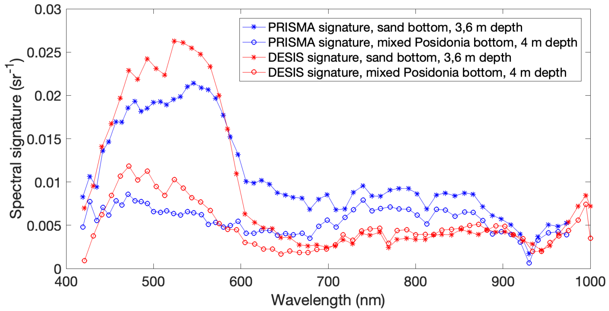
An example of PRISMA and DESIS reflectance spectra for two pixels, corresponding respectively to a sand area and to a mixed Posidonia area located at the seabed, are shown Figure 3. Pure Posidonia is only located in deep (>25 m) areas. The shape of the bottom reflectance is distorted by the light absorption by the water column.

It can be observed that beyond 700 nm, the information is not useful due to the high absorption by the water column.

2.2. Models

The semi-analytical radiative transfer model, the environmental noise probability model, and the water parameters probability model used in the study are briefly described here. In the following, lower case variables in bold are vectors, and uppercase variables in bold are matrices.

2.2.1. Semi-Analytical Radiative Transfer Model

The semi-analytical radiative transfer model that has been proposed by Lee et al. [15,52] is used here for modelling the water reflectance from the bio-optical properties of the water column (Equation (1)):

$$\mu ={\mathbf{r}}_{rs,\infty }\left[1-{\mathbf{K}}_C\right]+\frac{1}{\pi }{\mathbf{r}}_{0,B}{\mathbf{K}}_B,$$

(1)

where $\mathit{\mu }={[\mu \left({\lambda }_1\right)\dots \mu \left({\lambda }_L\right)]}^t$ is the modeled subsurface reflectance spectral vector, $\lambda$ is the wavelength, and L is the number of spectral bands. ${\mathbf{r}}_{0,B}$ is the bottom reflectance, ${\mathbf{r}}_{rs,\infty }$ is the reflectance of an infinitely deep water column, ${\mathbf{K}}_B$ and ${\mathbf{K}}_C$ are the attenuation matrices for the photons that interact (${\mathbf{K}}_B$) or not (${\mathbf{K}}_C$) with the bottom. ${\mathbf{K}}_B$ and ${\mathbf{K}}_C$ are expressed as follows (Equations (2) and (3)):

$$\begin{array}{c}\hfill {\mathbf{K}}_B=diag{\left[{\mathrm{e}}^{-(k_d\left({\lambda }_l\right)+k_u^b\left({\lambda }_l\right))H}\right]}_{l\in \left[1:L\right]}\end{array}$$

(2)

$$\begin{array}{c}\hfill {\mathbf{K}}_C=diag{\left[{\mathrm{e}}^{-(k_d\left({\lambda }_l\right)+k_u^c\left({\lambda }_l\right))H}\right]}_{l\in \left[1;L\right]}\end{array}$$

(3)

where ${\mathbf{k}}_{\mathbf{d}}$ is the attenuation coefficient of the water for the downwelling light, ${\mathbf{k}}_{\mathbf{u}}^{\mathbf{b}}$ (${\mathbf{k}}_{\mathbf{u}}^{\mathbf{c}}$) is the spectral attenuation coefficient of the water for the upwelling light, for the photons that interacts (resp. do not interacts) with the bottom. Two optical parameters, namely the absorption and the backscattering coefficients $a\left(\lambda \right)$ and $b_b\left(\lambda \right)$, depend on the water quality. The absorption and backscattering coefficients affect the subsurface reflectance through ${\mathbf{r}}_{\mathbf{rs},\infty }$ and the attenuation coefficients ${\mathbf{k}}_{\mathbf{d}}$, ${\mathbf{k}}_{\mathbf{u}}^{\mathbf{b}}$, ${\mathbf{k}}_{\mathbf{u}}^{\mathbf{c}}$. They are mainly dependent on three optically active constituents, phytoplankton pigments ($CHL$), colored dissolved organic matter ($CDOM$) and suspended particles matter ($SPM$). In this study, the expressions taken from [17,52] are used to express these parameters. The detailed expression of ${\mathbf{k}}_{\mathbf{d}}$, ${\mathbf{k}}_{\mathbf{u}}^{\mathbf{b}}$, and ${\mathbf{k}}_{\mathbf{u}}^{\mathbf{c}},\mathbf{a},{\mathbf{b}}_{\mathbf{b}}$ can be found in [64]. The unknown parameters are the water constituent concentrations $C_{CHL},C_{SPM}$, $C_{CDOM}$ (absorption coefficient at 440 nm), and the bathymetry designed by H. These four parameters can be estimated by inverting the radiative transfer Equation (1), using an optimization algorithm that minimizes the mean square error (MSE) between the measured ${\mathbf{r}}_{rs}$ and the modelled reflectance $\mathit{\mu }$. The bottom composition consists of a linear mixing of M pure materials which are representative of the seabed as follows:

$${\mathbf{r}}_{0,B}=\sum _{m=1}^M{a}_m{\mathbf{s}}_m.$$

(4)

Then the bottom can be estimated additionally, by estimating the mixing coefficients $a_m$. If the sum-to-one constraint ${\sum }_{m=1}^M{a}_m=1$ is applied to the mixing coefficients, they represent the abundance fraction of each material in a single pixel.

2.2.2. Environmental Noise

Previous works highlighted the importance of taking into account and modelling the variability of the observation [57]. The measured subsurface reflectance ${\mathbf{r}}_{rs}$ can be described by a Gaussian random vector (Equation (5)):

$${\mathbf{r}}_{rs}\sim N(\mathit{\mu },\mathbf{\Gamma }).$$

(5)

For each pixel of a given hyperspectral image, the mean value is $\mathit{\mu }$, as provided by the Equation (1), and the spectral covariance matrix $\mathbf{\Gamma }$ is supposed to be known and similar for each pixel. Practically, $\mathbf{\Gamma }$ can be obtained from the whole image. An equivalent formulation as Equation (5) could be as follows: ${\mathbf{r}}_{rs}=\mathit{\mu }+\mathbf{n}$, where $\mathbf{n}$ is an additive Gaussian noise with zero mean and a covariance equal to $\mathbf{\Gamma }$.

2.2.3. Water Column Parameters and Mixing Coefficients Variability

For the $CRB$ development, each water parameter that should be retrieved, i.e., $C_{CHL}$, $C_{CDOM},C_{SPM},H,a_m$, is considered as an unknown, but fixed parameter. For the $BCRB$ development, each parameter that should be retrieved, i.e., $C_{CHL},C_{CDOM},C_{SPM},H,a_m$, is considered as a random variable that follows an a priori known Gaussian law. All the parameters are supposed to be mutually independent [57]. The vector parameter $\mathbf{\Lambda }=\left[C_{CHL},C_{CDOM},C_{SPM},H,a_m\right]$ follows the Gaussian law:

$$\begin{array}{c}\hfill \mathbf{\Lambda }\sim N(\overline{\mathbf{\Lambda }},\mathbf{\Sigma }),\end{array}$$

(6)

where $\mathbf{\Sigma }=\left(\begin{array}{cccc}{\sigma }_{CHL}^2& 0& 0....& 0\\ 0& {\sigma }_{CDOM}^2& 0....& 0\\ 0& .& ....& 0\\ 0& & ....& 0\\ 0& 0& ....& {\sigma }_{a_m}^2\end{array}\right)$ is a diagonal matrix composed of the random parameters variances.

2.3. Methods

2.3.1. Water Column Bio-Optical Parameters and Seabed Composition

The water column parameters $\{C_{CHL},C_{CDOM},C_{SPM},H\}$ and the seabed composition coefficients $\{a_m,m=1\dots M\}$ were obtained by inverting the atmospherically corrected reflectance from DESIS and PRISMA images in the spectral range [420 nm–700 nm]. The inversion procedure was achieved by minimizing the Euclidian distance between the measured reflectance spectrum and the simulated one, using the $lsqcurvefit$ ^®MATLAB optimisation algorithm and Equation (1). The parameters were each optimized in a fixed range. The main constituents of the seabed are sand, Posidonia, and brown photophilic algae. Consequently, three mixing coefficients $a_1,a_2,a_3$ (see Equation (4)), are considered. The values of the retrieved geophysical products $\{C_{CHL},C_{CDOM},C_{SPM},H,a_1,a_2,a_3\}$ are used as input parameters for the calculation of the $CRB$ and $BCRB$, for each pixel and for each satellite image.

2.3.2. Covariance Estimation of the Environmental Noise

An estimate of the environment noise covariance is obtained directly from the hyperspectral images. It is considered that this noise includes the sensor noise as well as surface variations or variability in the atmospherical correction. A confident estimate of the covariance matrix of the environmental noise $\mathbf{\Gamma }$ is essential to obtain consistent $CRB$ and $BCRB$. The Automated Local Convergence Locator (ALCL) method [77] is an algorithm for locating suitable spatial areas for environmental noise retrieval in a remote sensing image. ALCL aims to find an area where the spectrally averaged standard deviation (std) of the reflectance computed over a square window does not change as the window size is incremented. Here, the ALCL criterion was modified as proposed in [64] to favor lower noise areas, and it was implemented to find a homogeneous area of optically deep water in the image.

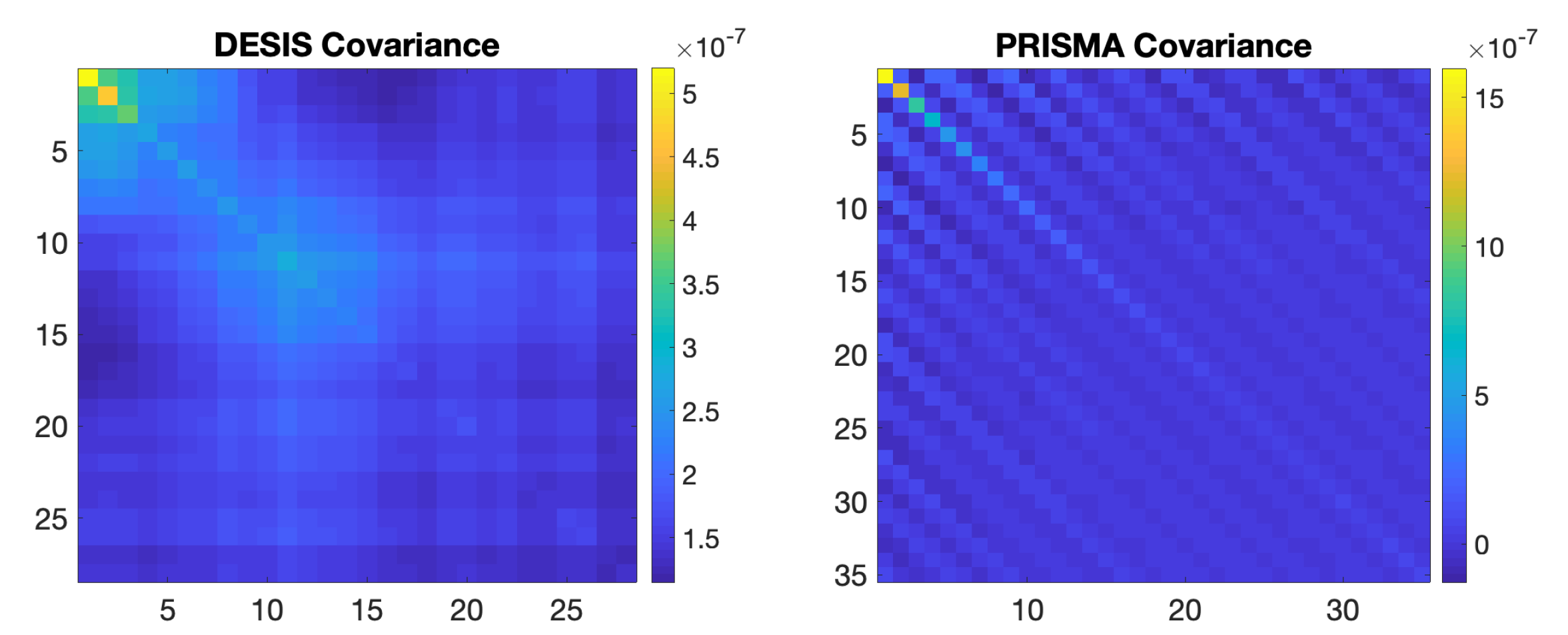
The DESIS (resp. PRISMA) covariance matrix is calculated on a rectangular area corresponding to the low values of the ALCL weighted map. It can be seen in Figure 4 that the estimated noise covariance is slighty higher for PRISMA than for DESIS. The mean value of the diagonal of the covariance matrix is $2.28E^{-7}$ for DESIS data and $2.39E^{-7}$ for PRISMA. This small difference can be due to the sensor SNR, but also to the sea surface effects and atmospherical conditions, since the dates of acquisition were not the same.

2.3.3. Development of the Cramér–Rao Bayesian Bounds Approach

The use of Cramér–Rao Bounds has been introduced for water column and bottom parameters in recent studies [62,63,64]. The $CRB$ can provide lower bounds for the estimation error of the unknown parameters, with fast computing time and for any chosen range of parameters. It can be an interesting technique for designing future satellite sensors. The $CRB$ and $BCRB$ calculus is the core of the presented work.

In [64], the semianalytical radiative transfer model of Lee has been already used to calculate $CRB$, although the parameterization of the water column constituents was somewhat different than the one we use here ($P,G,X$ instead of $C_{CHL},C_{CDOM},C_{SPM}$). $\mathbf{\Lambda }={\left[C_{CHL},C_{CDOM},C_{SPM},H,a_m(m=1\dots M)\right]}^T$ is the vector of unknown ocean color geophysical parameters to be retrieved from the remote-sensing observation ${\mathbf{r}}_{rs}$. The vector dimension is $N=4+M$ if no sum-to one constraint is applied, and $N=4+M-1$ if the sum-to one constraint is applied during the inversion. According to [69,70], the Fisher Information Matrix $\mathbf{J}$ is a square $N\times N$ matrix whose elements are defined as (Equation (7)):

$${\left[\mathbf{J}\left(\mathbf{\Lambda }\right)\right]}_{i,j}=\mathbb{E}\left[\left(\frac{\partial l\left({\mathbf{r}}_{rs}\right|\mathbf{\Lambda })}{\partial {\mathsf{\Lambda }}_i}\frac{\partial l\left({\mathbf{r}}_{rs}\right|\mathbf{\Lambda })}{\partial {\mathsf{\Lambda }}_j}\right)\right],$$

(7)

where $l\left({\mathbf{r}}_{rs}\right|\mathbf{\Lambda })$ is the log-Likelihood of ${\mathbf{r}}_{rs}$ given $\mathbf{\Lambda }$. The variance of any unbiased estimator ${\widehat{\mathsf{\Lambda }}}_i\left({\mathbf{r}}_{rs}\right)$ of an element ${\mathsf{\Lambda }}_i$ of $\mathbf{\Lambda }$ is bounded as follows (Equation (8)):

$$\mathbb{E}\left[{\left({\widehat{\mathsf{\Lambda }}}_i\left({\mathbf{r}}_{rs}\right)-{\mathsf{\Lambda }}_i\right)}^2\right]\ge {\left[\mathbf{J}{\left(\mathbf{\Lambda }\right)}^{-1}\right]}_{i,i}.$$

(8)

In the multivariate Gaussian case with mean $\mathit{\mu }$ and known covariance matrix $\mathbf{\Gamma }$, Equation (7) can be as follows [69,78] (Equation (9)):

$${\left[\mathbf{J}\left(\mathbf{\Lambda }\right)\right]}_{i,j}=\frac{\partial \mathit{\mu }}{\partial {\mathsf{\Lambda }}_i}{\mathbf{\Gamma }}^{-1}\frac{\partial \mathit{\mu }}{\partial {\mathsf{\Lambda }}_j}.$$

(9)

Here, the determination of the Fisher Information Matrix only requires the calculation of the derivatives $\frac{\partial \mu }{\partial {\mathsf{\Lambda }}_i}$. The Cramér–Rao Bounds of the parameters ${\mathsf{\Lambda }}_i$ are given by the diagonal elements of the inverse of the Fisher Information Matrix (Equation (10)):

$$CRB\left({\mathsf{\Lambda }}_i\right)={\left[\mathbf{J}{\left(\mathbf{\Lambda }\right)}^{-1}\right]}_{i,i}$$

(10)

Based on such a modelling approach, $CRB\left({\mathsf{\Lambda }}_i\right)$ includes the uncertainties associated to the considered Fisher Information Matrix, which only depends on the sensor radiometric specifications, bio-optical model, and environmental noise. Errors related to ground truth measurements, systematic corrections such as atmospherical corrections, inverse method or inaccurate modeling are not considered. $CRB\left({\mathsf{\Lambda }}_i\right)$ are the minimum uncertainties in ${\widehat{\mathsf{\Lambda }}}_i\left({\mathbf{r}}_{rs}\right)$ due to the environment noise (described by $\mathbf{\Gamma }$), and to the sensitivity of the model $\mathit{\mu }$ to the parameters variation (described by $\frac{\partial \mathit{\mu }}{\partial {\mathsf{\Lambda }}_j}$), for the specified wavelengths.

Some $a priori$ information is often available on the range of variation of the parameters. Previous studies showed the interest of including such knowledge when estimating the water column parameters, especially when the number of parameters increases [56]. In this case, the unknown parameters are considered as random parameters, with a known $apriori$ probability law. In a practical point of view, the inversion process used to estimate ${\mathsf{\Lambda }}_i\left({\mathbf{r}}_{rs}\right)$ is usually performed by minimizing the squared error between the modeled reflectance $\mathit{\mu }$ and the measured reflectance ${\mathbf{r}}_{rs}$. The minimum is searched in a bounded domain of variation for the parameters, which can be considered as a priori information. This information could be taken in consideration to determine a minimum error for the parameters estimation. The maximum $aposteriori$ Fisher Information Matrix ${\mathbf{J}}^{MAP}$, whose elements are defined in Equation (11), includes the $apriori$ information on the estimated parameters [69,70,79,80,81,82,83]:

$$\begin{array}{c}\hfill {\mathbf{J}}_{i,j}^{MAP}={\mathbb{E}}_{\mathbf{\Lambda }}{\left[\mathbf{J}\left(\mathbf{\Lambda }\right)\right]}_{i,j}+{\mathbb{E}}_{\mathbf{\Lambda }}\left[\frac{\partial log{P}_{\mathbf{\Lambda }}\left(\mathbf{\Lambda }\right)}{\partial {\mathsf{\Lambda }}_i}\frac{\partial log{P}_{\mathbf{\Lambda }}\left(\mathbf{\Lambda }\right)}{\partial {\mathsf{\Lambda }}_j}\right]\end{array}$$

(11)

where ${\mathbb{E}}_{\mathbf{\Lambda }}$ denotes expected value over the parameter vector $\mathbf{\Lambda }$. Here, the parameter ${\mathsf{\Lambda }}_i$ mean square error is bounded as:

$$E[{({\mathsf{\Lambda }}_i-{\widehat{\mathsf{\Lambda }}}_i)}^2]\ge {\left[{\left({\mathbf{J}}^{MAP}\right)}^{-1}\right]}_{i,i},$$

where ${\widehat{\mathsf{\Lambda }}}_i$ can be any nonbiased estimate of ${\mathsf{\Lambda }}_i$ [69].

If the parameter vector $\mathbf{\Lambda }$ follows a Gaussian law and if the noise $\mathbf{n}$ is additive and follows a Gaussian law as well, the two terms of ${\mathbf{J}}_{i,j}^{MAP}$ are given by Equation (12):

$$\begin{array}{c}\hfill {\mathbb{E}}_{\mathbf{\Lambda }}{\left[\mathbf{J}\left(\mathbf{\Lambda }\right)\right]}_{i,j}={\mathbb{E}}_{\mathbf{\Lambda }}\left[\frac{\partial \mu }{\partial {\mathsf{\Lambda }}_i}{\mathbf{\Gamma }}^{-1}\frac{\partial \mu }{\partial {\mathsf{\Lambda }}_j}\right]\\ \hfill {\mathbb{E}}_{\mathbf{\Lambda }}\left[\frac{\partial log{P}_{\mathbf{\Lambda }}\left(\mathbf{\Lambda }\right)}{\partial {\mathsf{\Lambda }}_i}\frac{\partial log{P}_{\mathbf{\Lambda }}\left(\mathbf{\Lambda }\right)}{\partial {\mathsf{\Lambda }}_j}\right]=d_{i,j}\end{array}$$

(12)

where $d_{i,j}$ denotes the $(i,j)$ element of ${\mathbf{\Sigma }}^{-1}$.

It has been shown that ${\mathbf{J}}^{MAP}$ can be approximated by [80,84,85]:

$$\begin{array}{c}\hfill {\mathbf{J}}^{MAP}={\mathbf{M}}^{\mathbf{T}}\mathbf{J}\mathbf{M}+{\mathbf{\Sigma }}^{-1}\end{array}$$

(13)

where $\mathbf{M}$ is the identity matrix $\mathbf{I}$ if each individual parameter follows a Normal distribution. The Bayesian Cramér–Rao bound ($BCRB$) is given by Equation (14).

$$BCRB\left({\mathsf{\Lambda }}_i\right)={\left[{\left({\mathbf{J}}^{MAP}\right)}^{-1}\right]}_{i,i}$$

(14)

3. Results

The products of the inversion of PRISMA and DESIS images are used to calculate their respective $BCR$ and $BCRB$. It should be highlighted that the aim of this work is not to obtain optimal inversion performance but to develop a method to obtain a reliable evaluation of the inversion performance.

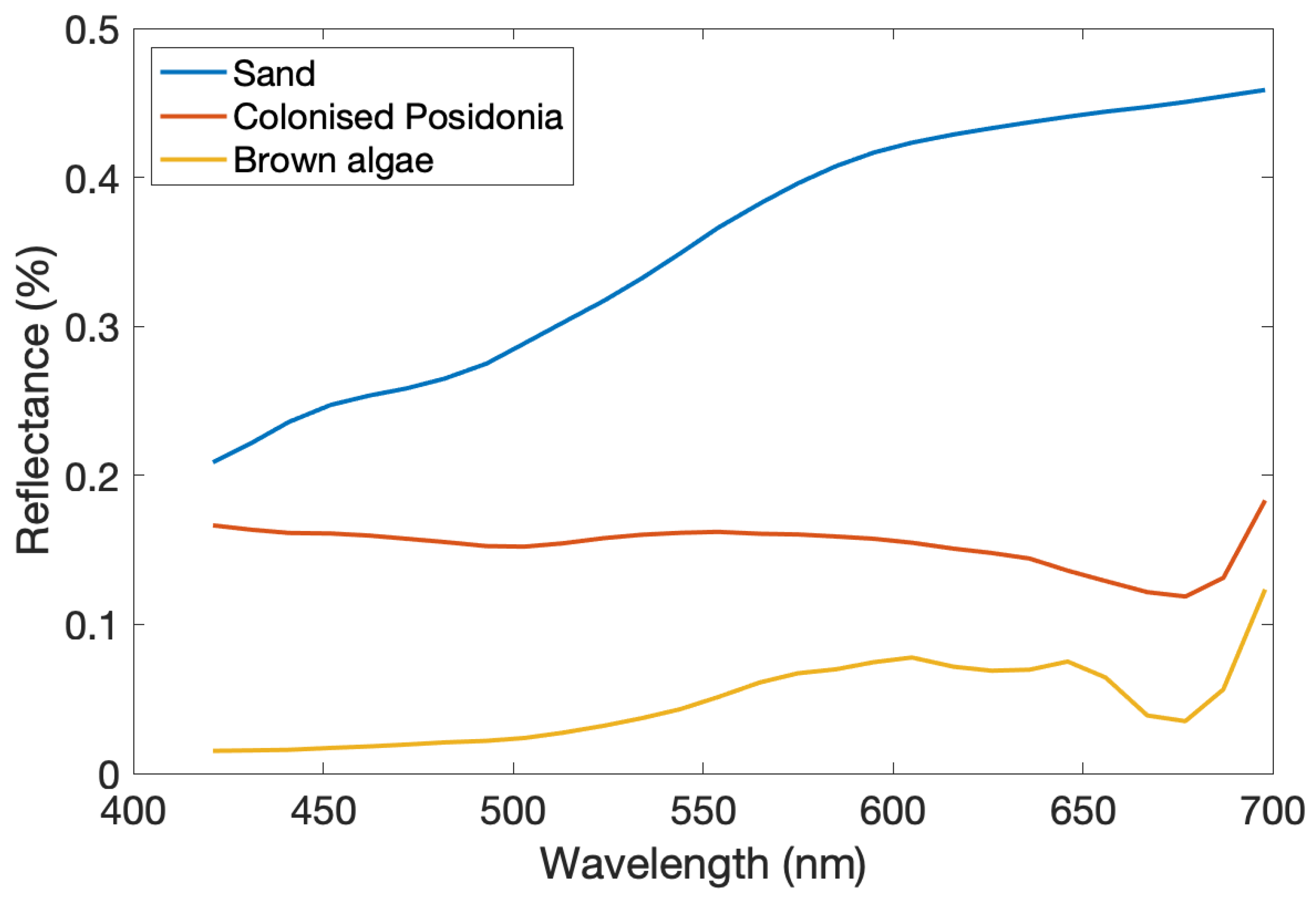
The water column parameters and the seabed composition are obtained for both images by inverting the reflectance data, using the radiative transfer equation presented in Equation (1) (see Section 2.3.1). The bottom reflectance is supposed to be a mixing of three materials, sand, Posidonia, and brown algae (see Section 2.1). Their spectral signatures are respectively referred to as ${\mathbf{s}}_1,{\mathbf{s}}_2,{\mathbf{s}}_3$, and the corresponding abundances (mixing coefficients) are respectively $a_1,a_2,a_3$. The mean square error between the modeled reflectance and the measured reflectance is optimized for each pixel N to retrieve the vector parameter ${\mathsf{\Lambda }}_i$. The spectral signatures used here are extracted from the same spectral library than those used in [59], which were collected in 2018 in the nearby area of Porquerolle island (France). Posidonia, brown algae and colonised Posidonia reflectance are the same than those used in [59], the sand spectrum magnitude is higher here. The reflectance spectra were obtained by dividing the ASD radiance of the benthic habitats by a Spectralon white field radiance, consequently they are in percentage.

The ^®$Litto3D$ bathymetry (see Section 2.1.1), referred to as z, is considered as the ground thruth, and is used to calculate the empirical error ($RMSE$) on bathymetry.

The sum-to-one constraint was applied to the abundances coefficients during the inversion, so only two abundance coefficients were considered as unknown parameters, resulting in six unknown parameters. Additional constraint such as limited domain of inversion for each parameter was applied during the optimisation procedure. The theoretical minimum bound for the estimation error of the water parameters have been performed for several cases: first, it was assumed that each parameter was estimated separately, all the others being known, so scalar $CRB$ and $BCRB$ ($CR{B}_1$ and $BCR{B}_1$) were calculated for each parameter of the vector $\mathbf{\Lambda }=\left[C_{CHL},C_{CDOM},C_{SPM},H,a_1,a_2\right]$. In a second step, the water composition $C_{CHL},C_{CDOM},C_{SPM},$ was supposed to be known, resulting in three parameters vectors Cramér–Rao Bounds being estimated ($CR{B}_3$ and $BCR{B}_3$). In a third step the $CRB$ and $BCRB$ for all the six parameters that were considered as simultaneously retrieved were calculated ($CR{B}_6$ and $BCR{B}_6$). This last configuration corresponds to that of the inversion. Since the $CRB$ and $BCRB$ provide minimum variance bounds, the square root of the $BCR$ and $BCRB$ are presented, to be consistent with a root mean square ($RMSE$) error. For the Bayesian $BCRB$, the $apriori$ distribution law of each parameter is approximated by a Gaussian distribution with a mean value equal to the value estimated in each pixel, and a variance equal to $\frac{q^2}{12}$, $q=b-a$, a and b being respectively the bounds of the research domain in the inversion algorithm for the estimation of each parameter.

The $CRB$ and the $BCRB$ relative to the depth are compared with empirical errors, obtained using the retrieved bathymetry denoted as H, and the ^®$Litto3D$ data, denoted as z, considered as ground truth. The $RMSE$ error for H is:

$$RMSE=\sqrt{\frac{1}{N}\sum _{n=1}^N{\left(H\left(n\right)-z\left(n\right)\right)}^2},$$

where $n=1\dots N$ is the index of the pixels in the inversion domain. The relative error $RE$ is obtained by using:

$$RE=\frac{1}{N}\sum _{n=1}^N\frac{H\left(n\right)-z\left(n\right)}{z\left(n\right)}.$$

3.1. CRB and BCRB for the PRISMA Image

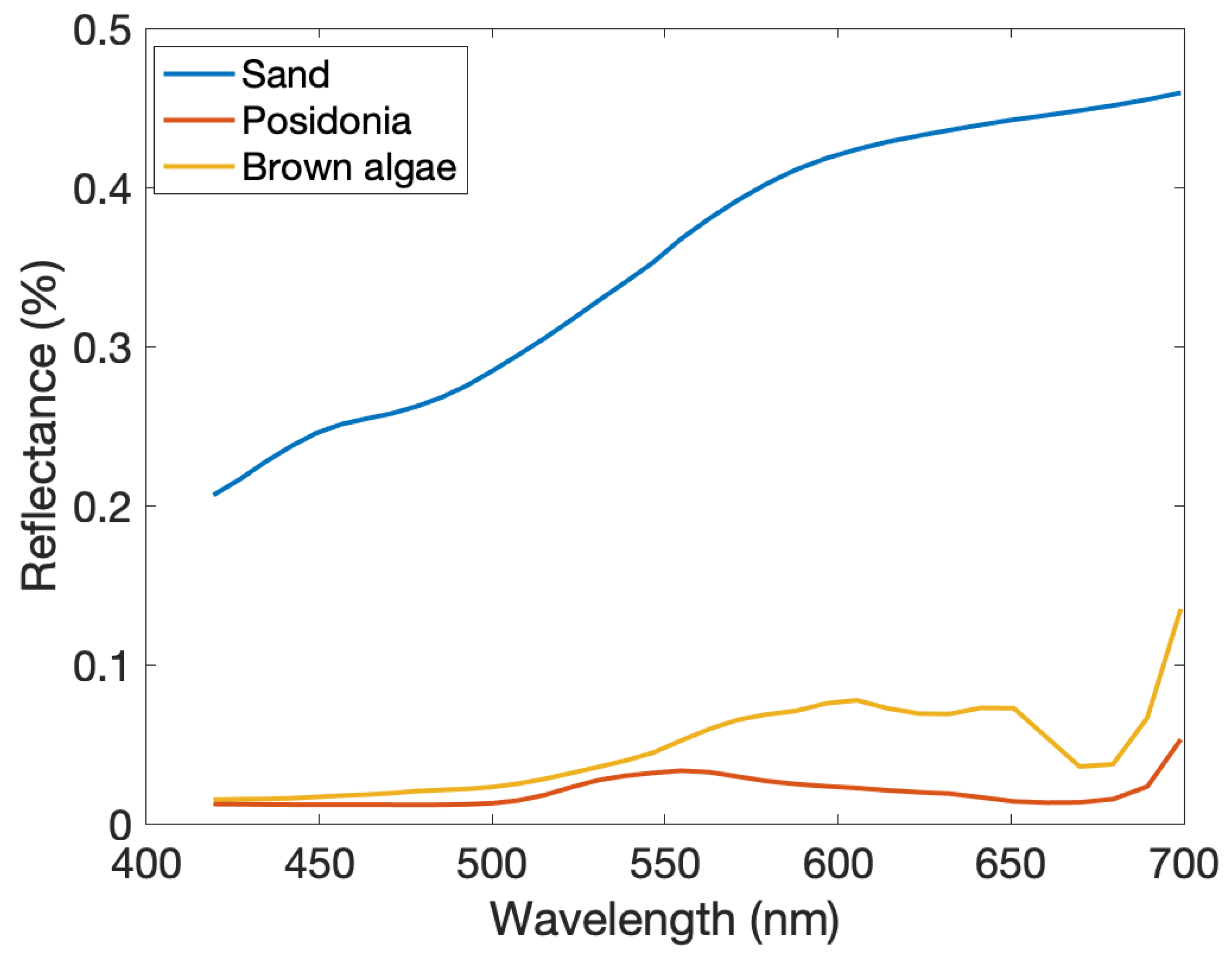
The PRISMA image has been masked for outliers pixels e.g., boats, and for pixels such as $z<3$ m or $z>30$ m (or alternatively $z>20$ m). Then, the inversion of the water parameters was performed in the inversion domain $\mathcal{D}{p}_{3-30}$ (resp. $\mathcal{D}{p}_{3-20}$), defined as the nonmasked pixels of the PRISMA image. The sum-to-one constraint was applied to the mixing coefficients $a_1,a_2,a_3$ during the inversion. The spectral signatures of sand, Posidonia and brown algage that were used for the inversion are shown in Figure 5.

3.1.1. Results for PRISMA Data Using the Inversion Domain $\mathcal{D}{p}_{3-30}$

The mean values obtained for the retrieval of the water column parameters (see Section 2.2) in the inversion domain $\mathcal{D}{p}_{3-30}$ are presented in

Table 1. PRISMA data: mean values of the retrieved water parameters in the inversion domain $\mathcal{D}{p}_{3-30}$, and bounds applied to the parameters during the inversion process.

Retrieved Parameter	H (m)	Cchl (mg.m${}^{-3}$)	Ccdom (m${}^{-1}$)	Cspm (g.m${}^{-3}$)	${\mathit{a}}_1$	${\mathit{a}}_2$	${\mathit{a}}_3$
Mean value	13.23	0.004	0.03	0.21	0.65	0.30	0.04
Bounds for inversion	[0–30]	[0–5]	[0–5]	[0–5]	[0–1]	[0–1]	[0–1]

:

The water quality shows mainly suspended matters ($SPM$) concentration, while low concentrations of Chlorophyll and organic dissolved matters are retrieved. The water is then considered as clear. The estimated bottom composition shows a majority of sand cover, while Posidonia abundance is around 30% and brown algae is rare.

The $CRB$ and $BCRB$ values, which are shown in

Table 2. PRISMA data: standard deviation ($std$) of the constraint applied to each parameter during the inversion, and square root of the mean $CR{B}_1$, (resp. $CR{B}_3$, $CR{B}_6$, $BCR{B}_1$, $BCR{B}_3$ and $BCR{B}_6$), obtained for the retrieved parameters in the domain $\mathcal{D}{p}_{3-30}$.

Parameter	H (m)	Cchl (mg.m${}^{-3}$)	Ccdom (m${}^{-1}$)	Cspm (g.m${}^{-3}$)	${\mathit{a}}_1$	${\mathit{a}}_2$
$apriori$ std	8.66	1.44	1.44	1.44	0.29	0.29
${\mathbf{CRB}}_{\mathbf{1}}^{\mathbf{0.5}}$	0.55	0.02	0.001	0.07	0.02	0.28
${\mathbf{CRB}}_{\mathbf{3}}^{\mathbf{0.5}}$	2.20	–	–	–	0.11	2.25
${\mathbf{CRB}}_{\mathbf{6}}^{\mathbf{0.5}}$	5.92	0.19	0.006	0.15	0.23	2.62
${\mathbf{BCRB}}_{\mathbf{1}}^{\mathbf{0.5}}$	0.49	0.02	0.001	0.07	0.02	0.11
${\mathbf{BCRB}}_{\mathbf{3}}^{\mathbf{0.5}}$	0.73	–	–	–	0.03	0.24
${\mathbf{BCRB}}_{\mathbf{6}}^{\mathbf{0.5}}$	1.37	0.14	0.005	0.14	0.08	0.27

, have been calculated for the retrieved values of the water column parameters in the inversion domain $\mathcal{D}{p}_{3-30}$. In order to take the sum-to-one constraint into account for the Cramér–Rao bounds calculus, only the two coefficients $a_1,a_2$ were considered as free parameters, the last one is retrieved by using $a_3=1-a_1-a_2$. $CR{B}_N^{0.5}$ is the root of the mean Cramér–Rao Bound over the whole area of the inversion domain, N is the number of parameters being retrieved (size of the vector $\mathsf{\Lambda }$). The $apriori$ standard deviation (std) for each parameter is the square root of the corresponding diagonal term of $\mathbf{\Sigma }$, as defined in Equation (6).

As expected, there is not much difference between the $CRB$ and the $BCRB$ for the case where only one parameter is unknown ($CR{B}_1$ and $BCR{B}_1$). This is because the estimation of only one unknown parameter while the others are supposed to be known, can be easily achieved, whether or not one has a priori knowledge. There is a higher difference betwen $CR{B}_1$ and $BCR{B}_1$ for the Posidonia abundance parameter $a_2$. The Posidonia may be difficult to estimate because of its low reflectance values compared to the sand ones. The Bayesian $BCRB$, which uses the $apriori$ information attached to the parameters, remains weak for the cases where three and six parameters are retrieved simultaneously, while the value of $CRB$ increase in those cases.

The empirical errors on the bathymetry, $RMSE$ and $RE$, are calculated for many depth ranges, in the case of all parameters being retrieved simultaneously (N = 6,

Table 3. PRISMA data: $RMSE$ error and relative error $RE$ (in bracket) for the retrieved bathymetry. The true depths are respectively comprised between [3 m–30 m], [3 m–6 m], [6 m–12 m], [12 m–30 m].

Depth Range	$\mathit{z}\in$ [3 m–30 m]	$\mathit{z}\in$ [3 m–6 m]	$\mathit{z}\in$ [6 m–12 m]	$\mathit{z}\in$ [12 m–30 m]
RMSE (m) and relative error RE (%)	8.67 (32%)	2.06 (35%)	1.23 ( 9%)	9.28 (34%)

):

The overall $RMSE$ is about 8.67 m for a depth range between 3 m and 30 m (about $32\%$ of relative error in mean). It is greater than both $CR{B}_6$ and $BCR{B}_6$, which are the theoretical lower bounds for the error. The calculation of $RMSE$ has also been carried out for three other depth ranges to better understand the uncertainties in the retrieval of the depth. It can be noted that the $RE$ is higher for shallowest and deepest waters: it is $35\%$ for $H\in$ [3 m–6 m] and $34\%$ for $H\in$ [12 m–30 m], while it is lower for intermediate depth values ($RMSE$ = 1.23 m, $RE$ = 9% for $H\in$ [6 m–12 m]). This latter point will be discussed in the following (Section 4).

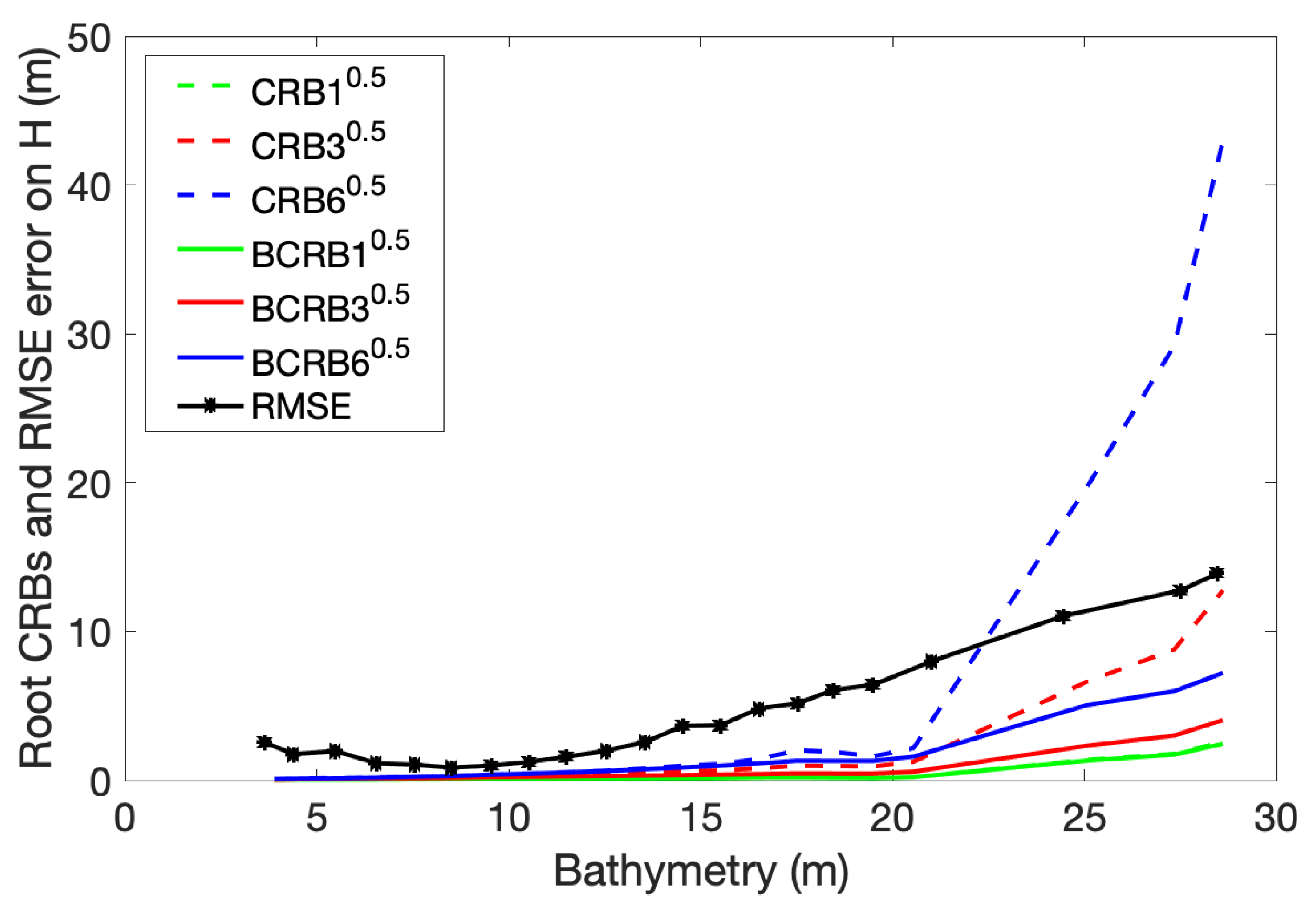
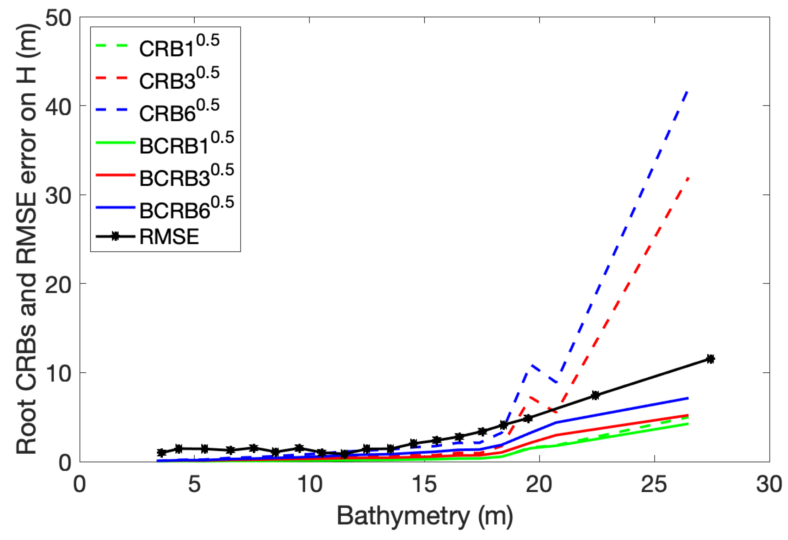
To better understand the variation of the $RMSE$ and $RE$ with the depth range as observed in Table 3, both Cramér–Rao Bounds and empirical $RMSE$ error for H are reported as a fuction of the bathymetry (Figure 6).

Note that since the $CRB$ are calculated using the oceanic parameters retrieved from the inversion process of PRISMA data, the $CRB$ and $BCRB$ values are dependent on the retrieved bathymetry H, while the empirical $RMSE$ error on the estimation of depth is reported as a function of the true bathymetry z, as provided by the ^®$Litto3D$ model. Both $CR{B}_N$ and $BCR{B}_N$ increase with the depth; $CR{B}_1$ is merged with $BCR{B}_1$, while the Bayesian $BCR{B}_N$ are lower than $CR{B}_N$ for 3 and 6 parameters estimated conjointly. The $RMSE$ empirical error vary in a different manner; it is quite high for depths between 3 m ($RMSE=2.5$ m) and 6 m ($RMSE=1.14$ m) meters, and decreases with the depth to attain a minimum value of 0.85 m at 8.5 m depth, to attain $1.23(RE=9\%)$ for the depth range $z\in$ [6 m–12 m]. The $RMSE$ is 1.23 m ($RE=9\%$) for the depth range $z\in$ [6 m–12 m], and increases beyond 12 m depth, to reach 14 m at 29 m depth ($RE=34\%$ in the range $z\in$ [12 m–29 m]). This will be discussed in the following (Section 4).

Beyond 20 m depth, the $CR{B}_6^{0.5}$ increases rapidly and gets higher than the empirical $RMSE$ error, which is not consistent with theory. Then, $CR{B}_6^{0.5}$ cannot be used to calculate minimum error bounds. Conversely, $BCR{B}_6^{0.5}$ remains lower $RMSE$ and increases in parallel with it beyond 20 m depth.

3.1.2. Results for PRISMA Data Using the Inversion Domain $\mathcal{D}{p}_{3-20}$

A second set of experiments was made for PRISMA image, to impose a more restrictive inversion domain and tighter constraints for the inversion. In the following, the inversion domain $\mathcal{D}{p}_{3-20}$ is defined as the nonoutsiders pixels in the domain $z\in$ [3 m–20 m]. The inversion bounds are set to [0 m–20 m] for H. The mean values of the retrieved parameters are given in

Table 4. PRISMA data: mean values of the retrieved water parameters in the inversion domain $\mathcal{D}{p}_{3-20}$, and bounds applied to the parameters during the inversion process.

Retrieved Parameter	H (m)	Cchl (mg.m${}^{-3}$)	Ccdom (m${}^{-1}$)	Cspm (g.m${}^{-3}$)	${\mathit{a}}_1$	${\mathit{a}}_2$	${\mathit{a}}_3$
Mean value	11.57	0.002	0.03	0.16	0.72	0.25	0.03
Bounds for inversion	[0–20]	[0–5]	[0–5]	[0–5]	[0–1]	[0–1]	[0–1]

.

In the domain $\mathcal{D}{p}_{3-20}$, as compared to $\mathcal{D}{p}_{3-30}$, the mean value of the bathymetry is lower, the water composition is similar except for the $SPM$ concentration which is lower. The sand estimated proportion is higher ($a_1=0.72$ instead of $a_1=0.65$).

The resulting $CR{B}_N$ and $BCR{B}_N$ are provided in

Table 5. PRISMA data: standard deviation ($std$) of the constraints applied to each parameter during the inversion, and square root of the mean $CR{B}_1$, (resp. $CR{B}_3$, $CR{B}_6$, $BCR{B}_1$, $BCR{B}_3$ and $BCR{B}_6$), obtained for the retrieved parameters in the domain $\mathcal{D}{p}_{3-20}$.

Parameter	H (m)	Cchl (mg.m${}^{-3}$)	Ccdom (m${}^{-1}$)	Cspm (g.m${}^{-3}$)	${\mathit{a}}_1$	${\mathit{a}}_2$
$apriori$   std	5.77	1.44	1.44	1.44	0.29	0.29
${\mathbf{CRB}}_{\mathbf{1}}^{\mathbf{0.5}}$	0.11	0.02	0.001	0.08	0.007	0.11
${\mathbf{CRB}}_{\mathbf{3}}^{\mathbf{0.5}}$	0.45	–	–	–	0.03	0.61
${\mathbf{CRB}}_{\mathbf{6}}^{\mathbf{0.5}}$	0.81	0.19	0.006	0.16	0.10	0.85
${\mathbf{BCRB}}_{\mathbf{1}}^{\mathbf{0.5}}$	0.11	0.02	0.001	0.08	0.007	0.09
${\mathbf{BCRB}}_{\mathbf{3}}^{\mathbf{0.5}}$	0.27	–	–	–	0.02	0.23
${\mathbf{BCRB}}_{\mathbf{6}}^{\mathbf{0.5}}$	0.62	0.14	0.005	0.15	0.07	0.26

:

The restriction of the inversion domain to $\mathcal{D}{p}_{3-20}$ affects only the values of the $CR{B}_N$ and $BCR{B}_N$ of H, $a_1$ and $a_2$, which are lower than those obtained in the domain ${\mathcal{D}}_{3-30}$, while the $CR{B}_N$ and $BCR{B}_N$ for the water parameters are in accordance with those obtained in the domain $\mathcal{D}{p}_{3-30}$.

The empirical errors on H are provided in

Table 6. PRISMA data: $RMSE$ error and relative error $RE$ on the bathymetry H, for depths respectively comprised between [3 m–20 m], [3 m–6 m], [6 m–12 m], [12 m–20 m].

Depth Range	$\mathit{z}\in$ [3 m–20 m]	$\mathit{z}\in$ [3 m–6 m]	$\mathit{z}\in$ [6 m–12 m]	$\mathit{z}\in$ [12 m–20 m]
RMSE (m) and relative error RE (%)	4.09 (20%)	2.06 (35%)	1.23 ( 9%)	4.72 (23%)

for several depth ranges:

Compared to the results of Table 3 (domain $\mathcal{D}{p}_{3-30}$), the errors in the range $z\in$ [3 m–6 m] and $z\in$ [6 m–12 m] do not change, while the errors in the ranges $z\in$ [3 m–20 m] and $z\in$ [12 m–20 m] are lower than for $z\in$ [3 m–30 m] and $z\in$ [12 m–30 m].

The $RMSE$ empirical error, $CRB$ and $BCRB$ for the bathymetry H are reported in Figure 7 as a function of the bathymetry:

The $CR{B}_N$ and $BCR{B}_N$ increase with depth, while the empirical $RMSE$ error first decreases in the interval $z\in$ [3 m–9 m], and increases after 9 m depth. The $CR{B}_6$ show some irregular variations after 15 m depth, while the $BCR{B}_6$ are lower and more regular and increase in parallel with the $RMSE$.

3.2. CRB and BCRB for DESIS Image

For DESIS image, the inversion domain is defined in the same way as for PRISMA image. The masked pixels could be somewhat different, because the day of acquisition was not the same and outliers pixels such as boats may have changed. In addition, the atmosphere conditions could also have changed, so despite the atmospherical correction it could lead to small variations. Last, water condition could have changed as well. The reference spectra used for the inversion are shown in Figure 8.

It can be seen that the Posidonia reflectance spectrum is not the same than the one used in the inversion of PRISMA image. For each image, the final selected signatures were the ones that provided the best final inversion results in terms of bottom habitats retrieval. For PRISMA image, colonised Posidonia was more representative than the fresh Posidonia signature which was used for DESIS image, because of the latter acquisition date in summer.

3.2.1. Results for DESIS Data Using the Inversion Domain $\mathcal{D}{d}_{3-30}$

The first set of experiments is performed for the pixels in the domain $\mathcal{D}{d}_{3-30}$. The imposed bounds in the inversion procedure are the same as for the PRISMA image.

The mean values of the retrieved water and seabed parameters over the inversion domain are reported in

Table 7. DESIS data: mean values of the retrieved water and seabed parameters in the domain $\mathcal{D}{d}_{3-30}$.

Retrieved Parameter	H (m)	Cchl (mg.m${}^{-3}$)	Ccdom (m${}^{-1}$)	Cspm (g.m${}^{-3}$)	${\mathit{a}}_1$	${\mathit{a}}_2$	${\mathit{a}}_3$
Mean value	13.90	5.36 ${10}^{-6}$	0.05	0.70	0.57	0.42	0.01
Bounds for inversion	[0–30]	[0–5]	[0–5]	[0–5]	[0–1]	[0–1]	[0–1]

:

The main conclusions on the water quality remain the same as for the PRISMA image: the suspended matters ($SPM$) concentration is moderate, while low concentrations of Chlorophyll and organic dissolved matters are retrieved. However, the mean value of the retrieved $SPM$ are higher (0.70 g.m${}^{-3}$ for DESIS and 0.21 g.m${}^{-3}$ for PRISMA). For the bottom cover, a little difference is noticeable with PRISMA results, the estimated sand cover is higher ($0.65$) and the Posidonia coverage is lower ($0.30$) for PRISMA data. It could be due to the use of the colonized Posidonia spectral signature which is more similar to sand spectra than fresh Posidonia spectral signature (used to invert PRISMA data).

The square root of the mean $CRB$ (resp. $BCRB$) obtained for the DESIS image are presented in

Table 8. DESIS data: Square root of the mean $CR{B}_1$, (resp. $CR{B}_3$, $CR{B}_6$, $BCR{B}_1$, $BCR{B}_3$ and $BCR{B}_6$), obtained for the retrieved parameters in the domain $\mathcal{D}{d}_{3-30}$.

Parameter	H (m)	Cchl (mg.m${}^{-3}$)	Ccdom (m${}^{-1}$)	Cspm (g.m${}^{-3}$)	${\mathit{a}}_1$	${\mathit{a}}_2$
$apriori$   std	8.66	1.44	1.44	1.44	0.28	0.28
${\mathbf{CRB}}_{\mathbf{1}}^{\mathbf{0.5}}$	0.31	0.03	0.001	0.08	0.02	0.04
${\mathbf{CRB}}_{\mathbf{3}}^{\mathbf{0.5}}$	1.28	–	–	–	0.26	0.51
${\mathbf{CRB}}_{\mathbf{6}}^{\mathbf{0.5}}$	2.15	0.12	0.009	0.17	0.67	1.34
${\mathbf{BCRB}}_{\mathbf{1}}^{\mathbf{0.5}}$	0.29	0.03	0.001	0.08	0.02	0.04
${\mathbf{BCRB}}_{\mathbf{3}}^{\mathbf{0.5}}$	0.57	–	–	–	0.12	0.18
${\mathbf{BCRB}}_{\mathbf{6}}^{\mathbf{0.5}}$	1.04	0.11	0.006	0.17	0.14	0.25

for the data in ${\mathcal{D}}_{3-30}$.

As the number of unknown parameters increases, the lower bounds increase, and the difference between $CRB$ and $BCRB$ also increases. It is observed that the use of $BCR{B}_3$ (resp. $BCR{B}_6$), leads to a decrease of around $50\%$ the $CRB$ for H. The $CR{B}_1$ for the Posidonia abundance $a_2$ is lower than for PRISMA data. It could be due to the colonized Posidonia spectral signature used, which has higher values than the fresh Posidonia signature used for PRISMA inversion. Generally the $CRB$ and the $BCRB$ are slightly below than for PRISMA data in the domain $\mathcal{D}{p}_{3-30}$, except for the $SPM$ concentration.

Table 9. DESIS data: $RMSE$ and $RE$ empirical errors on the bathymetry H for depths respectively comprised between [3 m–30 m], [3 m–6 m], [6 m–12 m], [12 m–30 m].

Depth Range	$\mathit{z}\in$ [3 m–30 m]	$\mathit{z}\in$ [3 m–6 m]	$\mathit{z}\in$ [6 m–12 m]	$\mathit{z}\in$ [12 m–30 m]
RMSE (m) and relative error RE (%)	6.96 (25%)	1.35 (25%)	1.20 ( 9.6%)	7.50 (27%)

presents the $RMSE$ and the $RE$ errors on the bathymetry H for several depth ranges:

The empirical errors are lower for DESIS data than for PRISMA data (see Table 3) in the ranges [3 m–6 m], and [12 m–30 m], but they are the same in the range [6 m–12 m]. Both Cramér–Rao Bounds and empirical $RMSE$ error for H are reported as a fuction of the bottom depth in Figure 9.

The $RMSE$ error increases after a minimum at 11 m depth, the $CR{B}_6$ and $CR{B}_3$ exceed the empirical error beyond 18 m depth, ans the $BCR{B}_6$ remains lower and parallel to the error.

3.2.2. Results for DESIS Data Using the Inversion Domain $\mathcal{D}{d}_{3-20}$

The mean values of the retrieved water and seabed parameters over the inversion domain are reported in

Table 10. DESIS data: mean values of the retrieved water and seabed parameters in the domain $\mathcal{D}{d}_{3-20}$.

Retrieved Parameter	H (m)	Cchl (mg.m${}^{-3}$)	Ccdom (m${}^{-1}$)	Cspm (g.m${}^{-3}$)	${\mathit{a}}_1$	${\mathit{a}}_2$	${\mathit{a}}_3$
Mean value	12.35	4.11 ${10}^{-7}$	0.06	0.79	0.62	0.37	0.008
Bounds for inversion	[0–20]	[0–5]	[0–5]	[0–5]	[0–1]	[0–1]	[0–1]

:

The main conclusions are similar as for the domain $\mathcal{D}{d}_{3-30}$, except for the bathymetry which is lower, for the $SPM$ concentration which slightly higher and the sand abundance which is higher. Compared to the PRISMA image, the concentration of $SPM$ is higher, while the mean value of sand abundance is lower and the Posidonia abundance is higher.

The square root of the mean $CRB$ (resp. $BCRB$) obtained for the DESIS image are presented in

Table 11. DESIS data: standard deviation ($std$) of the constraints applied to the parameters during the inversion, and square root of the mean $CR{B}_1$, (resp. $CR{B}_3$, $CR{B}_6$, $BCR{B}_1$, $BCR{B}_3$ and $BCR{B}_6$), obtained for the retrieved parameters in the domain $\mathcal{D}{d}_{3-20}$.

Parameter	H (m)	Cchl (mg.m${}^{-3}$)	Ccdom (m${}^{-1}$)	Cspm (g.m${}^{-3}$)	${\mathit{a}}_1$	${\mathit{a}}_2$
$apriori$ std	5.77	1.44	1.44	1.44	0.28	0.28
${\mathbf{CRB}}_{\mathbf{1}}^{\mathbf{0.5}}$	0.24	0.03	0.002	0.09	0.02	0.04
${\mathbf{CRB}}_{\mathbf{3}}^{\mathbf{0.5}}$	0.85	–	–	–	0.21	0.38
${\mathbf{CRB}}_{\mathbf{6}}^{\mathbf{0.5}}$	1.61	0.11	0.009	0.20	0.52	1.04
${\mathbf{BCRB}}_{\mathbf{1}}^{\mathbf{0.5}}$	0.23	0.03	0.002	0.09	0.02	0.04
${\mathbf{BCRB}}_{\mathbf{3}}^{\mathbf{0.5}}$	0.47	–	–	–	0.11	0.17
${\mathbf{BCRB}}_{\mathbf{6}}^{\mathbf{0.5}}$	0.82	0.10	0.006	0.19	0.14	0.24

for the inversion domain $\mathcal{D}{d}_{3-20}$.

As the number of unknown parameters increases, the lower bounds increase, and the difference between $CRB$ and $BCRB$ also increases. The root of the mean $CBR$ for H for the case where three and six parameters are unknown is 0.85 m, and 1.61 m respectively. It is observed that the use of the Bayesian approach $BCRB$, which takes into consideration the available $apriori$ knowledge on the range of variation of the oceanic parameters, leads to a $50\%$ reduction of the $CR{B}_{\mathrm{3,6}}^{0.5}$ for the two latter cases.

The empirical $RMSE$ and $RE$ errors on H are calculated in the domain $\mathcal{D}{d}_{3-20}$ (

Table 12. DESIS data: $RMSE$ and $RE$ empirical errors on the bathymetry H, for depths respectively comprised between [3 m–20 m], [3 m–6 m], [6 m–12 m], [12 m–20 m].

Depth Range	$\mathit{z}\in$ [3 m–20 m]	$\mathit{z}\in$ [3 m–6 m]	$\mathit{z}\in$ [6 m–12 m]	$\mathit{z}\in$ [12 m–20 m]
RMSE (m) and relative error RE (%)	2.71 (15%)	1.35 (25%)	1.20 (9%)	3.09 (16%)

):

The root mean square error $RMS{E}_{3-20}$ = 2.71 m, is higher than both $CR{B}_6^{0.5}$ and $BCR{B}_6^{0.5}$. The minimum error is in the depth domain $z\in$ [6 m–12 m] (1.2 m, 9%). The error increases for low bathymetry and high bathymetry.

The $CRB$ and $BCRB$ for H are presented as a function of the retrieved depth H in Figure 10, together with the $RMSE$ as a function of the ground truth depth z.

The $CR{B}_N$ and the $BCR{B}_N$ increase with the depth. The $apriori$ knowledge (i.e., $BCRBi$) does not lead to a decrease of the bounds when a single parameter is retrieved ($BCR{B}_1$ and $CR{B}_1$), while the Bayesian bounds are lower for the cases of three and six retrieved parameters. The empirical error is quite high for a weak bathymetry $z\in$ [3 m–8 m] (around 1.3 m), decreases for z between 8 m and 13 m, and increases for $z>14$ m. For depths higher than 18 m, the $CR{B}_N$ increase rapidly and exceed the $RMSE$, while the $BCR{B}_N$ remain lower and increase in parallel with the $RMSE$.

Figure 7, Figure 9 and Figure 10, show that the standard $CRB$ approach cannot be used to estimate the minimum bounds in the considered inversion domain, because it may exceed the $RMSE$ in some cases. The $BCR{B}_6$, which include the same $apriori$ knowledge on the parameters than the $RMSE$, provides a better idea of what minimal bounds could be expected when estimating water constituents and seabed parameters.

4. Discussion

4.1. Interpretation of the Variation of $RMSE$ with the Depth

4.1.1. Lower Depths

Both empirical errors estimated from PRISMA and DESIS images show a nonexpected variation for lshallow depths. It is well known that the error on depth estimation increases with the depth [63], except for very shallow water (less than 0.5 cm depth for moderately turbid waters). Here the error on H presents a minimum around 8 m depth, while it should regularly increase from 1 m depth. The $CR{B}_6$ and $BCR{B}_6$ do not present this minimum, they regularly increase, as expected.

Let us examine the error sources taken in consideration in the development of the $CRB$ and $BCRB$ lower bounds. The error sources are the environmental noise (covariance matrix), the sensitivity of the model to a variation of the parameters, and the number of parameters that needs to be simultaneously retrieved (i.e., size of the Fisher Information matrix). The $CRB$ and $BCRB$ also depend on the set of wavelengths used. Other sources of error could be examined, such as the spatial resolution. In Section 2.1, where the data are presented, it is shown that the depth increases rapidly with the distance from the beach (Figure 2). The spatial resolution is 30 m for both $PRISMA$ and $DESIS$ images. The depth slope, which is calculated between the pixel #1 and the pixel #4 of the depth profile shown Figure 2, leads to a variation of 2.3 m depth per pixel (square of 30 m × 30 m of the scene) in mean. However, in the pixelwise inversion procedure developed to obtain the vector parameter $\mathsf{\Lambda }$, the depth is assumed to be constant over one pixel. If the depth varies inside a single pixel, there could be a confusion between depth (H) and bottom composition ($a_m$). Then, the simultaneaous estimation of all the parameters is no longer reliable and the error increases due to the rough spatial resolution. The error is higher for lower depths because the relative depth variation within one pixel is higher for very shallow water than for deeper water, making the estimation very challenging at lower depths.

Briefly, the results shown Figure 5, Figure 6, Figure 8 and Figure 9, and in Table 3, Table 6, Table 9 and Table 12, which report a higher error for shallow pixels, show that the spatial resolution of the satellite sensor is a critical parameter for estimating the depth in shallow and steep coastal areas.

4.1.2. Higher Depths

For the intermediate depth interval [6 m–12 m], the influence of the bottom slope gets relatively lower within one pixel because the reflectance model is less sensitive to a variation of depth of a few meters. In addition, the bottom composition has lower influence at these depths. This could explain that the $RMSE$ is lower (around $9\%$ of relative error for all the treated cases). For the depth range [12 m–20 m] (resp. [12 m–30 m]), the error increases. Following Lee’s model given in Equation (1), the attenuation matrices ${\mathbf{K}}_B$ and ${\mathbf{K}}_C$ decrease as the water column height H increases, so the water reflectance tends to that of ${\mathbf{r}}_{rs,\infty }$ at higher depths. Then, very poor information on the depth H could be derived. As a result, the retrieval error on H increases at higher depths, the bottom being barely visible. $RE$ is $23\%$ (resp. $34\%)$ for PRISMA data and $RE$ is $16\%$ (resp. $23\%$) for DESIS data. DESIS data seem to be more robust than PRISMA data for the deepest areas; however, the $RMSE$ and $RE$ errors are very dependent on outliers pixels, which can be masked or not in the inversion procedure. Therefore, it is not possible to draw any final conclusion about the comparison of the PRISMA and DESIS sensors performances.

4.2. Comparison between $CR{B}_N$ and $BCR{B}_N$

For the depth estimation, as previously mentioned, there is no significant difference between $CR{B}_1$ and $BCR{B}_1$. This is because the inversion of one parameter is not challenging in the context of the noise of PRISMA (and DESIS) data and shallow clear water. For such a case, the introduction of $apriori$ knowledge does not change the accuracy of the estimate. Of course the expected $RMSE$ error of estimation, as well as the $CR{B}_N$ and the $BCR{B}_N$, depend on the number of unknown parameters N that should be estimated simultaneously. The differences between $CR{B}_N$ and $BCR{B}_N$ appear for three parameters unknown, and increase with the number of retrieved parameters (6 parameters). The $CR{B}_N$ become unstable and diverge for the higher depths and the higher number of parameters. The $CR{B}_N$ can exceed the $RMSE$ for challenging conditions such as a low signal to noise level, and a high number of unknown parameters. This is not consistent with theory which claims that $CRB$ represent the lower bounds, which can only be reached using a Maximum Likelihood estimator, when all the sources of variability are correctly modeled. Here, some sources of error are not taken into account, such as radiative transfer model errors, noise model errors, spectral signatures reliability and variability, and also the influence of the spatial resolution. The $CR{B}_N$ should be significantly less than the errors. Beyond z = 13 m, the $RMSE$ increases with an approximately constant slope for all experiments, because the optimization algorithm is driven by the imposed bounds of the parameters. The $BCR{B}_N$, which take into account this a priori knowledge, remain always lower than the $RMSE$ and increase in parallel with it from around 17 m depth.

For the water constituents concentrations $C_{CHL},C_{CDOM},C_{SPM}$, there is not much difference between the $CR{B}_N$ and $BCR{B}_N$ for all the configuration tested (Table 2, Table 5, Table 8 and Table 11). This could be due to the values of the imposed bounds in the optimization, which are quite large compared to the actual values of the parameters; consequently the a priori knowledge is weak and does not significantly decrease the $BCR{B}_N$ in comparison with the $CR{B}_N$.

Our results show that the $CR{B}_6$ are not able to represent the minimum bounds for the error obtained for six parameters unknown, while $BCR{B}_6$ has the advantages to represent those minimum bounds. The models and the method used to develop the Bayesian version of the $CRB$, although they are based on some assumptions (see Section 2), could be used to derive a good approximation of minimum bounds for estimated water column parameters and seabed composition.

4.3. Difference between PRISMA and DESIS Sensors

The results of the inversion of PRISMA and DESIS sensors are regionally consistent. They both show presence of $SPM$, low concentrations of $CHL$ and $CDOM$, a major coverage of sand and Posidonia, and very few brown algae. However, some differences were observed.

The $CR{B}_N$ and the $BCR{B}_N$ depend on the parameters value. It is not possible to compare PRISMA and DESIS sensors performances based on the $CR{B}_N$ and the $BCR{B}_N$ obtained for the products of the inversion of the two images presented in Figure 1, because the retrieved parameters are different for each image. To compare the lower bounds for the two sensors, the water column parameters and the bottom composition should be the same. One simulation using the same values of all the parameters representative of the scene and the same bottom reflectance for both sensors has thus been carried out. The characteristics of the two sensors such as wavelengths between 420 nm and 700 nm and covariance matrices are the ones that have been used previously in Section 3. The parameters values used for simulation are presented in

Table 13. Values of the water parameters and bottom abundances used in the simulation.

Retrieved Parameter	H (m)	Cchl (mg.m${}^{-3}$)	Ccdom (m${}^{-1}$)	Cspm (g.m${}^{-3}$)	${\mathit{a}}_1$	${\mathit{a}}_2$	${\mathit{a}}_3$
Mean value	[1–20]	0.001	0.05	0.5	0.65	0.30	0.05

:

The resulting $BCR{B}_6$ as a function of the depth are shown Figure 11.

Generally, the $BCRB$ are slightly lower for $DESIS$ than for $PRISMA$, except for the $SPM$ concentrations. For the bathymetry H, the lower bounds increase with the depth, varying from 0.01 m (1%) at 1 m depth for both sensors, to 2.24 m (11%) for PRISMA and 1.80 m (9%) for DESIS at 20 m depth. The relative difference between the PRISMA and DESIS $BCRB$ is $20\%$ at 20 m depth. The lower bounds for the water column composition ($CHL$, $CDOM$, $SPM$) increase at lower depth, due to the lack of information about the water composition because the water layer is too thin. This is an expected result [64]. The bounds associated with $CHL$ concentrations are very high compared to the $CHL$ concentrations used for the simulations. This is consistent with the previous results shown Table 2, Table 5, Table 8 and Table 11. In fact, very little $CHL$ is present in the water column; thus, it could not be detected. This could lead to an associated $BCRB$ higher than the parameter value $C_{CHL}$. The relative difference between PRISMA and DESIS $BCRB$ is around $30\%$. For the $CDOM$ concentration, which is near zero in Figure 11, the values of the $BCRB$ are between 0.012 m${}^{-1}$ and 0.007 m${}^{-1}$ for PRISMA, and between 0.009 m${}^{-1}$ and 0.005 m${}^{-1}$ for DESIS. There is a minimum around 7 m depth, and the $BCRB$ both increase at lower and higher bathymetry. The $BCRB$ are low compared to the parameter value (about $10\%$), and the relative difference between PRISMA and DESIS $BCRB$ is around $20\%$. The $BCRB$ associated with $SPM$ are higher than the concentrations for low bathymetry ($H<$ 3 m). They decrease rapidly up to 6 m, and it continues to decrease slowly beyond 6 m. The $BCRB$ are higher for DESIS between 2 m and 14 m, and the two sensors $BCRB$ curves superimposed beyond 14 m. The relative difference is around $20\%$ at 10 m depth. The $BCRB$ for the abundances increase with the depth, and for $a_2$ it tends towards the $apriori$ std 0.28 m (it should be the same for $a_1$ for deepest bottoms).

Briefly, the minimum error bounds $BCRB$ for PRISMA and DESIS sensors are of the same magnitude, even if it appears a relative difference between $10\%$ and $30\%$ in the range of parameters used in favor of DESIS, except for the $SPM$ minimum bound which is lower for PRISMA.

5. Conclusions and Perspectives

In this paper, a Bayesian Cramér–Rao Bounds approach has been proposed for assessing the water column parameters estimation from hyperpsectral satellite data acquired over a coastal environment. Two sets of satellite data have been used, namely DESIS and PRISMA data. For both cases the $RMSE$ empirical error between ground truth and retrieved bathymetry was compared to the standard Cramér–Rao Bounds and to the Bayesian Cramér–Rao Bounds, for the case where up to six water colum and bottom parameters should be retrieved by the inversion algorithm. The standard $CRB$ approach was shown to go beyond the empirical error for the most challenging retrieval configurations such as those which imply retrieving various water parameters and bathymetry simultaneously. The Bayesian $BCRB$ approach that takes into account the inversion constraints applied to the retrieved parameters, is proved to be more robust than $CRB$, lower than the empirical error and to vary in parallel with it in the most challenging cases. The proposed $BCRB$ approach is then able to quantify uncertainties that could be reached when inverting the sea surface remote sensing reflectance to derive ocean color parameters. The mains outcomes of this study are as follow:

-

A method for deriving Bayesian Cramér–Rao bounds ($BCRB$) of water column parameters and seabed composition is proposed

-

The obtained $BCRB$ are consistent with empirical measures of errors for the retrieved bathymetry

-

The standard $CRB$ are not always consistent with the empirical measures of errors for the retrieved bathymetry

-

The spatial resolution of the satellite sensor is crucial for having reliable parameters estimation in shallow and steep areas

-

The PRISMA and DESIS sensors have comparable minimum bounds performances

The proposed $BCRB$ approach does not take into account the loss of performance due to rough spatial resolution. Future works could consist in modeling the uncertainty that is induced by the spatial resolution.

References

1. Vahtmäe, E.; Paavel, B.; Kutser, T. How much benthic information can be retrieved with hyperspectral sensor from the optically complex coastal waters? J. Appl. Remote Sens. 2020, 14, 016504. [Google Scholar] [CrossRef]
2. Alevizos, E. A Combined Machine Learning and Residual Analysis Approach for Improved Retrieval of Shallow Bathymetry from Hyperspectral Imagery and Sparse Ground Truth Data. Remote Sens. 2020, 12, 3489. [Google Scholar] [CrossRef]
3. Pérez-Ruzafa, A.; Marcos, C.; Pérez-Ruzafa, I. Mediterranean coastal lagoons in an ecosystem and aquatic resources management context. Phys. Chem. Earth Parts A/B/C 2011, 36, 160–166. [Google Scholar] [CrossRef]
4. Le Fur, I.; De Wit, R.; Plus, M.; Oheix, J.; Simier, M.; Ouisse, V. Submerged benthic macrophytes in Mediterranean lagoons: Distribution patterns in relation to water chemistry and depth. Hydrobiologia 2017, 808, 175–200. [Google Scholar] [CrossRef]
5. Zaldívar, J.-M.; Viaroli, P.; Newton, A.; De Wit, R.; Ibañez, C.; Reizopoulou, S.; Somma, F.; Razinkovas, A.; Basset, A.; Holmer, M.; et al. Eutrophication in Transitional Waters: An Overview. Transit. Waters Monogr. 2008, 2, 1–78. [Google Scholar]
6. Hochberg, E.J. Coral Reefs: An Ecosystem in Transition. Remote Sensing of Coral Reef Processes. In Coral Reefs: An Ecosystem in Transition; Dubinsky, Z., Stambler, N., Eds.; Springer: Dordrecht, The Netherlands, 2011; pp. 25–35. [Google Scholar]
7. Hedley, J.D.; Roelfsema, C.M.; Chollett, I.I.; Harborne, A.R.; Heron, S.F.; Weeks, S.J.; Skirving, W.J.; Strong, A.E.; Eakin, C.M.; Christensen, T.R.; et al. Remote sensing of coral reefs for monitoring and management: A review. Remote Sens. 2016, 8, 118. [Google Scholar] [CrossRef]
8. Chauvaud, S.; Bouchon, C.; Maniere, R. Remote sensing techniques adapted to high resolution mapping of tropical coastal marine ecosystems (coral reefs, seagrass beds and mangrove). Int. J. Remote Sens. 1998, 19, 3625–3639. [Google Scholar] [CrossRef]
9. Jaubert, J.; Chisholm, J.; Minghelli-Roman, A.; Marchioretti, M.; Morrow, J.; Ripley, H. Re-evaluation of the extent of caulerpa taxifolia development in the northern mediterranean using airborne spectrographic sensing. Mar. Ecol. Prog. Ser. 2003, 263, 75–82. [Google Scholar] [CrossRef]
10. Garcia, R.A.; Fearns, P.R.; McKinna, L.I. Detecting trend and seasonal changes in bathymetry derived from HICO imagery: A case study of Shark Bay, Western Australia. Remote Sens. Environ. 2014, 147, 186–205. [Google Scholar] [CrossRef]
11. Jaba Deva Krupa, A.; Samiappan, D.; Hemalatha, V. Techniques for seabed mapping using underwater hyperspectral imaging: A survey. Int. J. Pure and Appl. Math. 2018, 118, 11–30. [Google Scholar]
12. Werdell, P.J.; Franz, B.A.; Bailey, S.W.; Feldman, G.C.; Boss, E.; Brando, V.E.; Dowell, M.; Hirata, T.; Lavender, S.J.; Lee, Z.; et al. Generalized ocean color inversion model for retrieving marine inherent optical properties. Appl. Opt. 2013, 52, 2019–2037. [Google Scholar] [CrossRef]
13. Mobley, C. Light and Water: Radiative Transfer in Natural Waters; Academic Press: San Diego, CA, USA, 1994. [Google Scholar]
14. Chami, M.; Lafrance, B.; Fougnie, B.; Chowdhary, J.; Harmel, T.; Waquet, F. Osoaa: A vector radiative transfer model of coupled atmosphere-ocean system for a rough sea surface application to the estimates of the directional variations of the water leaving reflectance to better process multi-angular satellite sensors data over the ocean. Opt. Express 2015, 23, 27829. [Google Scholar]
15. Lee, Z.; Carder, K.; Mobley, C.; Steward, R.; Patch, J. Hyperspectral remote sensing for shallow waters. i. a semianalytical model. Appl. Opt. 1998, 37, 6329–6338. [Google Scholar] [CrossRef]
16. Maritorena, S.; Morel, A.; Gentili, B. Diffuse reflectance of oceanic shallow waters—Influence of water depth and bottom albedo. Limnol. Oceanogr. 1994, 39, 1689–1703. [Google Scholar] [CrossRef]
17. Dekker, A.G.; Phinn, S.R.; Anstee, J.; Bissett, P.; Brando, V.E.; Casey, B. Intercomparison of shallow water bathymetry, hydro-optics, and benthos mapping techniques in Australian and Caribbean coastal environments. Limnol. Oceanol. Methods 2011, 9, 396–425. [Google Scholar] [CrossRef]
18. Hedley, J.; Roelfsema, C.; Phinn, S. Efficient radiative transfer model inversion for remote sensing applications. Remote Sens. Environ. 2009, 113, 2527–2532. [Google Scholar] [CrossRef]
19. Goodman, J.A. Hyperspectral Remote Sensing of Coral Reefs: Deriving Bathymetry, Aquatic Optical Properties and a Benthic Spectral Unmixing Classification Using Aviris Data in the Hawaiian Islands. Ph.D. Dissertation, Hydrologic Sciences, Department of Land, Air and Water Resources, University of California, Davis, CA, USA, 2004. [Google Scholar]
20. Goodman, J.; Ustin, S. Classification of benthic composition in a coral reef environment using spectral unmixing. J. Appl. Remote Sens. 2007, 1, 1. [Google Scholar]
21. Torres-Madronero, M.; Velez-Reyes, M.; Goodman, A. Underwater unmixing and water optical properties retrieval using hyciat. In Proceedings of SPIE: Imaging Spectrometry XIV; SPIE Optical Engineering + Applications: San Diego, CA, USA, 2009; Volume 7457. [Google Scholar]
22. Marcello, J.; Eugenio, F.; Martín, J.; Marqués, F. Seabed Mapping in Coastal Shallow Waters Using High Resolution Multispectral and Hyperspectral Imagery. Remote Sens. 2018, 10, 1208. [Google Scholar] [CrossRef]
23. Hochberg, E.; Atkinson, M. Capabilities of remote sensors to classify coral, algae, and sand as pure and mixed spectra. Remote Sens. Environ. 2003, 85, 174–189. [Google Scholar] [CrossRef]
24. Lee, Z.; Carder, K. Effect of spectral band numbers on the retrieval of water column and bottom properties from ocean color data. Appl. Opt. 2002, 41, 2191–2201. [Google Scholar] [CrossRef]
25. Minghelli-Roman, A.; Chisholm, J.; Marchioretti, M.; Jaubert, J. Discrimination of coral reflectance spectra in the red sea. Coral Reef 2002, 21, 307–314. [Google Scholar] [CrossRef]
26. Lee, Z.; Weidemann, A.; Arnone, R. Combined effect of reduced band number and increased bandwidth on shallow water remote sensing: The case of worldview 2. IEEE Trans. Geosc. Remote Sens. 2013, 51, 2577–2586. [Google Scholar] [CrossRef]
27. Hochberg, E.; Atkinson, M.; Andréfouët, S. Spectral reflectance of coral reef bottom-types worldwide and implications for coral reef remote sensing. Remote Sens. Environ. 2003, 85, 159–173. [Google Scholar] [CrossRef]
28. Botha, E.; Brando, V.; Anstee, J.; Dekker, A.; Sagar, S. Increased spectral resolution enhances coral detection under varying water conditions. Remote Sens. Environ. 2013, 131, 247–261. [Google Scholar] [CrossRef]
29. Emberton, S.; Chittka, L.; Cavallaro, A.; Wang, M. Sensor capability and atmospheric correction in ocean colour remote sensing. Remote Sens. 2016, 8, 1. [Google Scholar] [CrossRef]
30. Odermatt, D.; Gitelson, A.; Brando, V.E.; Schaepman, M. Review of constituent retrieval in optically deep and complex waters from satellite imagery. Remote Sens. Environ. 2012, 118, 116–126. [Google Scholar] [CrossRef]
31. Matthews, M.W. A current review of empirical procedures of remote sensing in inland and near-coastal transitional waters. Int. J. Remote Sens. 2011, 32, 6855–6899. [Google Scholar] [CrossRef]
32. Hestir, E.L. Measuring freshwater aquatic ecosystems: The need for a hyperspectral global mapping satellite mission. Remote Sens. Environ. 2015, 735, 181–195. [Google Scholar] [CrossRef]
33. Hedley, J.; Roelfsema, C.; Phinn, S.; Mumby, P. Environmental and sensor limitations in optical remote sensing of coral reefs: Implications for monitoring and sensor design. Remote Sens. 2012, 4, 271–302. [Google Scholar] [CrossRef]
34. NASA/CASEI. Available online: https://impact.earthdata.nasa.gov/casei/instrument/CASI/ (accessed on 16 March 2023).
35. Jet Propulsion Laboratory, California Institute of Technology. Available online: https://aviris.jpl.nasa.gov/ (accessed on 16 March 2023).
36. HYSPEX. Available online: https://www.hyspex.com/ (accessed on 16 March 2023).
37. TELECOM PARIS. Available online: https://www.telecom-paris-alumni.fr/fr/revue/article/the-iss-has-a-new-colorful-eye/3450 (accessed on 16 March 2023).
38. Loizzo, R. Prisma: The Italian hyperspectral mission. In Proceedings of the Procedure of IEEE International Symposium on Geoscience and Remote Sensing (IGARSS), Symposium, Valencia, Spain, 22–27 July 2018; pp. 175–178. [Google Scholar]
39. Rast, M.; Painter, T.H. Earth observation imaging spectroscopy for terrestrial systems: An overview of its history, techniques, and applications of its missions. Surv. Geophys. 2019, 40, 303–331. [Google Scholar] [CrossRef]
40. Minghelli, A.; Vadakke-Chanat, S.; Chami, M.; Guillaume, M.; Migne, E.; Grillas, P.; Boutron, O. Estimation of Bathymetry and Benthic Habitat Composition from Hyperspectral Remote Sensing Data (BIODIVERSITY) Using a Semi-Analytical Approach. Remote Sens. 2021, 13, 1999. [Google Scholar] [CrossRef]
41. Remer, L.A.; Davis, A.; Mattoo, B.; Levy, R.S.; Kalashnikova, O.; Coddington, O.; Chowdhary, J.; Knobelspiesse, K.; Xu, X.; Ahmad, Z.; et al. Retrieving Aerosol Characteristics From the PACE Mission, Part 1: Ocean Color Instrument. Front. Earth Sci. 2019, 7, 2296–6463. [Google Scholar] [CrossRef]
42. Giardino, C.; Bresciani, M.; Braga, F.; Fabbretto, A.; Ghirardi, N.; Pepe, M.; Gianinetto, M.; Colombo, R.; Cogliati, S.; Ghebrehiwot, S.; et al. First Evaluation of PRISMA Level 1 Data for Water Applications. Sensors 2020, 20, 4553. [Google Scholar] [CrossRef]
43. Bresciani, M.; Giardino, C.; Fabbretto, A.; Pellegrino, A.; Mangano, S.; Free, G.; Pinardi, M. Application of New Hyperspectral Sensors in the Remote Sensing of Aquatic Ecosystem Health: Exploiting PRISMA and DESIS for Four Italian Lakes. Resources 2022, 11, 8. [Google Scholar] [CrossRef]
44. Niroumand-Jadidi, M.; Bovolo, F.; Bruzzone, L. Water Quality Retrieval from PRISMA Hyperspectral Images: First Experience in a Turbid Lake and Comparison with Sentinel-2. Remote Sens. 2020, 12, 3984. [Google Scholar] [CrossRef]
45. Gauto, V.; Ferral, A.; Bonansea, M.; Farías, A.; Scavuzzo, M.; Cardozo, O.; Giardino, C. First results of PRISMA satellite data applied to water quality monitoring in Argentina. In Proceedings of the 2022 IEEE Biennial Congress of Argentina (ARGENCON), San Juan, Argentina, 7–9 September 2022; pp. 1–8. [Google Scholar]
46. Salama, M.S.; Stein, A. Error decomposition and estimation of inherent optical properties. Appl. Opt. 2009, 48, 4947–4962. [Google Scholar] [CrossRef]
47. Moore, T.S.; Campbell, J.W.; Dowell, M.D. A class-based approach to characterizing and mapping the uncertainty of the MODIS ocean chlorophyll product. Remote Sens. Environ. 2009, 113, 2424–2430. [Google Scholar] [CrossRef]
48. Gregg, W.W. Assimilation of SeaWiFS ocean chlorophyll data into a three-dimensional global ocean model. J. Mar. Syst. 2008, 69, 205–225. [Google Scholar] [CrossRef]
49. Lee, Z.; Arnone, R.; Hu, C.; Werdell, P.J.; Lubac, B. Uncertainties of optical parameters and their propagations in an analytical ocean color inversion algorithm. Appl. Opt. 2010, 49, 369–381. [Google Scholar] [CrossRef]
50. Pahlevan, N.; Sarkar, S.; Franz, B.A. Uncertainties in coastal ocean color products: Impacts of spatial sampling. Remote Sens. Environ. 2016, 181, 14–26. [Google Scholar] [CrossRef]
51. Lyzenga, D.R. Passive remote sensing techniques for mapping water depth and bottom features. Appl. Opt. 1978, 17, 379–383. [Google Scholar] [CrossRef]
52. Lee, Z.; Carder, K.L.; Mobley, C.D.; Steward, R.G.; Patch, J.S. Hyperspectral remote sensing for shallow waters: 2. deriving bottom depths and water properties by optimization. Appl. Opt. 1999, 38, 3831–3843. [Google Scholar] [CrossRef]
53. Brando, V.; Anstee, J.; Wettle, M.; Dekker, A.; Phinn, S.; Roelfsema, C. A physics based retrieval and quality assessment of bathymetry from suboptimal hyperspectral data. Remote Sens. Environ. 2009, 113, 755–770. [Google Scholar] [CrossRef]
54. Jay, S.; Guillaume, M. A novel maximum likelihood based method for mapping depth and water quality from hyperspectral remote-sensing data. Remote Sens. Environ. 2014, 147, 121–132. [Google Scholar] [CrossRef]
55. McKinna, L.I.; Fearns, P.R.; Weeks, S.J.; Werdell, P.J.; Reichstetter, M.; Franz, B.A.; Shea, D.M.; Feldman, G.C. A semi-analytical ocean color inversion algorithm with explicit water column depth and substrate reflectance parameterization. J. Geophys. Res. Oceans 2015, 120, 1741–1770. [Google Scholar] [CrossRef]
56. Jay, S.; Guillaume, M. Regularized estimation of bathymetry and water quality using hyperspectral remote sensing. Int. J. Remote Sens. 2016, 37, 263–289. [Google Scholar] [CrossRef]
57. Jay, S.; Guillaume, M.; Minghelli, A.; Deville, Y.; Chami, M.; Lafrance, B.; Serfaty, V. Hyperspectral remote sensing of shallow waters: Considering environmental noise and bottom intra-class variability for modeling and inversion of water reflectance. Remote Sen. Environ. 2017, 200, 352–367. [Google Scholar] [CrossRef]
58. Thompson, D.; Hochberg, E.; Asner, G.; Green, R.; Knapp, D.E.; Cay Gao, B.; Garcia, R.; Gierach, M.; Lee, Z.; Maritorena, S.; et al. Airborne mapping of benthic reflectance spectra with bayesian linear mixtures. Remote Sens. Environ. 2017, 200, 18–30. [Google Scholar] [CrossRef]
59. Minghelli, A.; Vaddake-Chanat, S.; Chami, M.; Guillaume, M.; Peirache, M. Benefit of the potential future hyperspectral satellite sensor (BIODIVERSITY) for improving the determination of water column and seabed features in coastal zones. IEEE J. Sel. Top. Appl. Earth Ob. Remote Sens. 2021, 14, 1222–1232. [Google Scholar] [CrossRef]
60. Wang, P.; Boss, E.S.; Roesler, C. Uncertainties of inherent optical properties obtained from semianalytical inversions of ocean color. Appl. Opt. 2005, 44, 4074–4085. [Google Scholar] [CrossRef]
61. Werdell, P.J.; McKinna, L.I.W.; Boss, E.; Ackleson, S.G.; Craig, S.E.; Gregg, W.W.; Lee, Z.; Maritorena, S.; Roesler, C.S.; Rousseaux, C.S.; et al. An overview of approaches and challenges for retrieving marine inherent optical properties from ocean color remote sensing. Prog. Oceanogr. 2018, 160, 186–212. [Google Scholar] [CrossRef] [PubMed]
62. Jay, S.; Guillaume, M. Estimation of water column parameters with a maximum likelihood approach. In Proceedings of the 3rd IEEE Workshop on Hyperspectral Image and Signal Processing: Evolution in Remote Sensing, IEEE, Lisbon, Portugal, 6–9 June 2011; pp. 1–4. [Google Scholar]
63. Jay, S. Estimation et déTection en Imagerie Hyperspectrale: Application aux Environnements Côtiers. Ph.D. Thesis, Ecole Centrale de Marseille, Marseille, France, 2012. Available online: http://www.theses.fr/2012ECDM0004 (accessed on 16 March 2023).
64. Jay, S.; Guillaume, M.; Chami, M.; Minghelli, A.; Deville, Y.; Lafrance, B.; Serfaty, V. Predicting minimum uncertainties in the inversion of ocean color geophysical parameters based on Cramer-Rao bounds. Opt. Express 2018, 26, A1–A18. [Google Scholar] [CrossRef]
65. Cramér, H. Mathematical Methods of Statistics; Princeton University Press: Princeton, NJ, USA, 1946. [Google Scholar]
66. Rao, C. Information and the accuracy attainable in the estimation of statistical parameters. Bull. Calcutta Math. Soc. 1945, 37, 81–89. [Google Scholar]
67. Fréchet, M. Sur l’extension de certaines évaluations statistiques au cas de petits échantillons. Rev. Inst. Int. Statist. 1943, 11, 182–205. [Google Scholar] [CrossRef]
68. Darmois, G. Sur les limites de la dispersion de certaines estimations. Rev. Int. Inst. Statist. 1945, 13, 9–15. [Google Scholar] [CrossRef]
69. Van Trees, H.L. Detection, Estimation, and Modulation Theory—Part I; John Wiley and Sons: New York, NY, USA, 1968. [Google Scholar]
70. Garthwaite, P.H.; Jolliffe, I.T.; Jones, B. Statistical Inference; Oxford University: Oxford, UK, 2002. [Google Scholar]
71. Kay, S.M. Fundamentals of Statistical Signal Processing: Estimation Theory; Prentice Hall: Englewood Cliffs, NJ, USA, 1993; p. 47. [Google Scholar]
72. Louvart, L.; Grateau, C. The Litto3D Project. In Proceedings of the IEEE Oceans 2005—Europe International Conference, Brest, France, 20–23 June 2005; Volume 2, pp. 1244–1251. [Google Scholar]
73. ®LITTO3D, IGNF_SHOM_LITTO3Dr_1-0. 2008. Available online: https://www.geoportail.gouv.fr/donnees/litto3d (accessed on 16 March 2023).
74. Kotchenova, S.Y.; Vermote, E.F.; Matarrese, R.; Klemm, F.J., Jr. Validation of a vector version of the 6S radiative transfer code for atmospheric correction of satellite data. Part I: Path Radiance. Appl. Opt. 2006, 45, 6726–6774. [Google Scholar] [CrossRef] [PubMed]
75. Gordon, H.R.; Wang, M. Retrieval of water-leaving radiance and aerosol optical thickness over the oceans with SeaWiFS: A preliminary algorithm. Appl. Opt. 1994, 3, 443–452. [Google Scholar] [CrossRef]
76. Siegel, D.A.; Wang, M.; Maritorena, S.; Robinson, W. Atmospheric correction of satellite ocean color imagery: The black pixel assumption. Appl. Opt. 2000, 39, 3582–3591. [Google Scholar] [CrossRef]
77. Wettle, M.; Brando, V.E.; Dekker, A.G. A methodology for retrieval of environmental noise equivalent spectra applied to four hyperion scenes of the same tropical coral reef. Remote Sens. Environ. 2004, 93, 188–197. [Google Scholar] [CrossRef]
78. Stoica, P.; Moses, R.L. Spectral Analysis of Signals; Pearson Prentice Hall: Upper Saddle River, NJ, USA, 2005; Volume 452. [Google Scholar]
79. Gill, R.D.; Levit, B.Y. Applications of the van Trees inequality: A Bayesian Cramér-Rao bound. Bernoulli 1995, 1, 59–79. [Google Scholar] [CrossRef]
80. Tichavsky, P.; Muravchik, C.; Nehorai, A. Posterior Cramer Rao Bounds for Discrete-Time Nonlinear Filtering. IEEE Trans. Signal Process. 1998, 46, 5. [Google Scholar] [CrossRef]
81. Manry, M.T.; Hsieh, C.-H.; Dawson, M.S.; Fung, A.K.; Apollo, S.J. Cramer Rao Maximum A-Posteriori Bounds on Neural Network Training Error for Non-Gaussian Signals and Parameters. Int. J. Intell. Control Syst. 1996, 1, 381–391. [Google Scholar] [CrossRef]
82. Yu, Q.; Apollo, S.J.; Manry, M.T. MAP Estimation and the Multilayer Perceptron. In Proceedings of the 1993 IEEE Workshop on Neural Networks for Signal Processing, Linthicum Heights, MD, USA, 6–9 September 1993; pp. 30–39. [Google Scholar]
83. Clarkson, E. Relation between Bayesian Fisher information and Shannon information for detecting a change in a parameter. J. Opt. Soc. Am. A Opt. Image Sci. Vis. 2019, 36, 1209–1214. [Google Scholar] [CrossRef] [PubMed]
84. Nguyen, T.H.T.; Nguyen, T.T.; Mentré, F. Individual Bayesian information matrix for predicting estimation error and shrinkage of individual parameters accounting for data below the limit of quantification: Bayesian information matrix accounting for data below LOQ. Pharm. Res. 2017, 17, inserm-01549693. [Google Scholar]
85. Combes, F.P.; Retout, S.; Frey, N.; Mentré, F. Prediction of shrinkage of individual parameters using the bayesian information matrix in non-linear mixed effect models with evaluation in pharmacokinetics. Pharm. Res. 2013, 30, 2355–2367. [Google Scholar] [CrossRef]
Figure 1. Red-Green-Blue (RGB) image acquired by (a) DESIS sensor (13 June 2021) and (b) PRISMA sensor (14 August 2021).
Remotesensing 15 02242 g001
Figure 2. L i t t o 3 D  data: (a) bathymetry between 0 m and 30 m; the red vertical line in column 250 is the location of the profile; (b) depth profile corresponding to the red line, from the beach up to −30 m.
Remotesensing 15 02242 g002
Figure 3. Spectral signatures from DESIS and PRISMA images, for the same two pixels, corresponding respectively to a sand seabed area and to a mixed (70%) Posidonia seabed area.
Remotesensing 15 02242 g003
Figure 4. Covariancematrices estimated on an homogeneous area of DESIS and PRISMA images.
Remotesensing 15 02242 g004
Figure 5. Reflectance spectra of benthic habitat used for the inversion of PRISMA image.
Remotesensing 15 02242 g005
Figure 6. PRISMA data: root mean square of the Cramér–Rao and the Bayesian Cramér–Rao bounds as a function of the estimated bathymetry, and empirical error ( R M S E ) as a function of the true bathymetry, for the inversion domain  D p 3 30 .
Remotesensing 15 02242 g006
Figure 7. PRISMA data: root mean square of the Cramér–Rao and Bayesian Cramér–Rao bounds as a function of the estimated bathymetry, and empirical  R M S E  error as a function of the true bathymetry, for the inversion domain  D p 3 20 .
Remotesensing 15 02242 g007
Figure 8. Reflectance spectra of benthic habitat used for the inversion of DESIS image.
Remotesensing 15 02242 g008
Figure 9. DESIS data: root mean square of the Cramér–Rao and the Bayesian Cramér–Rao bounds as a function of the estimated bathymetry, and empirical  R M S E  error as a function of the true bathymetry, for data in the domain  D d 3 30 .
Remotesensing 15 02242 g009
Figure 10. DESIS data: root mean square of the Cramér–Rao bounds and the Bayesian Cramér–Rao bounds and empirical error ( R M S E ) as a function of the bathymetry, for the domain  D d 3 20 .
Remotesensing 15 02242 g010
Figure 11. Comparison between  B C R B  obtained for PRISMA and DESIS sensors, using 6 retrieved parameters and simulated data; (a) for H, (b) for  C H L , C D O M , S P M , (c) for  a 1 , a 2 .
Remotesensing 15 02242 g011