Article

Analysis of Spatial and Temporal Criteria for Altimeter Collocation of Significant Wave Height and Wind Speed Data in Deep Waters

by
Ricardo M. Campos
1,2
1
Cooperative Institute for Marine and Atmospheric Studies (CIMAS), University of Miami, 4600 Rickenbacker Causeway, Miami, FL 33149, USA
2
NOAA Atlantic Oceanographic and Meteorological Laboratory (AOML), 4301 Rickenbacker Causeway, Miami, FL 33149, USA
Remote Sens. 2023, 15(8), 2203; https://doi.org/10.3390/rs15082203
Submission received: 24 March 2023 / Revised: 17 April 2023 / Accepted: 19 April 2023 / Published: 21 April 2023

Abstract

:
This paper investigates the spatial and temporal variability of significant wave height (Hs) and wind speed (U10) using altimeter data from the Australian Ocean Data Network (AODN) and buoy data from the National Data Buoy Center (NDBC). The main goal is to evaluate spatial and temporal criteria for collocating altimeter data to fixed-point positions and to provide practical guidance on altimeter collocation in deep waters. The results show that a temporal criterion of 30 min and a spatial criterion between 25 km and 50 km produce the best results for altimeter collocation, in close agreement with buoy data. Applying a 25 km criterion leads to slightly better error metrics but at the cost of fewer matchups, whereas using 50 km augments the resulting collocated dataset while keeping the differences to buoy measurements very low. Furthermore, the study demonstrates that using the single closest altimeter record to the buoy position leads to worse results compared to the collocation method based on temporal and spatial averaging. The final validation of altimeter data against buoy observations shows an RMSD of 0.21 m, scatter index of 0.09, and correlation coefficient of 0.98 for Hs, confirming the optimal choice of temporal and spatial criteria employed and the high quality of the calibrated AODN altimeter dataset.

1. Introduction

Long-term observations of significant wave height (Hs) and 10 m wind speed (U10) are crucial for several activities and studies, including extreme value analysis [1,2,3], climate studies [4,5,6,7,8], the validation of hindcast data [9,10,11] and forecast products [10,11,12,13,14], data assimilation [15,16,17,18], and the development of post-processing bias correction algorithms [19]. Satellite altimetry has emerged as one of the most valuable sources of reliable information regarding Hs and U10, following the launch of GEOSAT in 1985 [20]. Since 2002 [21], a large number of satellites and quality-controlled altimeter datasets with high accuracy have become available [22,23,24], which now provide more than 20 years of observations with great temporal and spatial coverage. Zieger et al. [25] described that altimeter satellites (especially Ku-band) are capable of measuring Hs and U10 with accuracy similar to metocean buoys. Additionally, compared to moored buoys, altimeters allow much larger datasets with global domains instead of single-point positions, being important for large-scale studies and the assessment and optimization of wave models.
Due to the polar orbit, satellites revisit a site once every 10 to 35 days with tracks separated by 100 to 200 km [26], so whenever altimeter measurements are compared against buoy data or model data at fixed grid points and regular time-steps, position and time must be carefully analyzed. For instance, every location along the Jason-3 ground-track is measured approximately every 9.9 days [27]. In this context, a maximum distance, both in time and space, centered at the buoy (or model grid point) position has to be considered for the altimeter collocation process—defining criteria for spatial and temporal separation between such observations. Next, two options are possible: (1) the single closest altimeter record to the fixed buoy’s position is selected or (2) the average is calculated for along-track altimeter records attending a space–time criteria. Zieger et al. [25] argues that the spatial average provides a more statistically stable comparison than a single-point observation—which is the approach chosen by most of the studies in the area, e.g., [4,7,13,19,20,23,25,28,29,30,31,32,33,34,35,36].
The aforementioned papers were based on the widely used criteria of altimeter tracks within 50 km of the buoy and the overpass within 30 min of the buoy recording data. Such values are well established and have been derived from the fundamental studies of Monaldo [28] and Dobson et al. [20], who deeply analyzed time and space sampling differences and the impact of the temporal and spatial proximity of altimeter tracks to buoy observations. In 1988, Monaldo [28] found that 30 min time separation leads to expected uncertainty of 0.3 m for Hs and 0.5 m/s for U10. Using the 50 km/30 min criteria, he found that the accuracy of GEOSAT data compared against buoys was within 0.5 m for Hs and between 1.8 and 2.0 m/s for U10.
Considering the very high accuracy of recent satellite data [23] as well as new hindcast and forecast products recently released, it is important to reassess such criteria, including buoys with longer durations and more satellite missions which are now available. This is an important task to ensure the temporal and spatial variabilities associated with altimeter collocation do not exceed the expected error of high-performance modeling products and new satellite missions. Therefore, based on the recent demand described above, the present paper uses long-term observations from buoys and altimeters to investigate time and space sampling differences and to evaluate different criteria for altimeter collocation. The main goal is to analyze the impact of several spatial and temporal criteria on the comparison of altimeters with buoys while looking at the resulting number of matchups generated in the process. The averaging method is also investigated, and a practical discussion is conducted to support future studies involving altimeter collocation to fixed-point positions.

2. Materials and Methods

An important aspect of this type of study is to select reliable observations with long durations and very few gaps to obtain robust and meaningful statistics. The temporal analyses were based on buoy data, while satellite data were used for the spatial analyses, followed by a final spatio-temporal discussion. This work is restricted to deep-water observations far from the coast. The primary goal is to investigate Hs, but U10 is also included due to its high correlation and direct impact on Hs. All the web links to access the data used in this work are included at the end of this manuscript.

2.1. Buoy Data

Buoy data from the National Data Buoy Center [37] were selected because of the center’s consistent data processing and quality control over the stations and due to the large number of buoys with long durations. Following Ribal and Young [23], only buoys more than 50 km offshore were used. It is impressive how some stations have been measuring continuously since the 1970s and 1980s with minor gaps. A thorough inspection of the buoy datasets with the longest duration, the smallest discontinuities, and stable positions led to the selection of 11 NDBC buoys, shown in Figure 1. The proper continuity of observations throughout the years without many periods of absent data is important for the autocorrelation function and spectral analysis. The 11 buoys were distributed over four clusters, illustrated with different colors in Figure 1. Table 1 presents the information on each buoy. These stations gather a valuable dataset with more than 200 thousand records (hourly data) per buoy, covering more than 30 years’ worth of observations.
In addition to the data cleaning and quality control implemented by NDBC, an additional quality control was further applied, based on [37,38,39], to ensure the final time-series had reliable information on Hs and U10. All buoys selected were at least 150 km from the nearest coast, with water depths above 800 m. The wind profile power law was applied to convert U10 from the anemometer height (usually between 3 to 5 m) to the 10 m level, following Equation (1) [40].
u u r = ( z z r ) α
where u is the wind speed (m/s) at height z (m), and u r is the known wind speed at reference height z r . The constant α is the friction coefficient, which is a function of the topography at a specific site—commonly assumed to be equal to 1/7. Instead of 0.14, Hsu et al. [41] suggest 0.10 is more appropriate for lakes and oceans, and Jung et al. [42] and DNV-RP-C205 [40] recommend 0.12 for open sea with waves—which has been applied in the present study.
The uncertainties and errors associated with buoy data of Hs and U10 have been discussed by several authors (e.g., [43,44,45,46,47,48,49]). Bowler [43] describes that observation errors from heave–pitch–roll wave buoys depend on the type of accelerometer, buoy size and hull, the mooring system, and the metocean conditions. Liu et al. [44] found average errors from different types of buoys between 3.47% and 3.79% for Hs. Using Wavescan, SeaWatch Mini II, Directional Waverider, and TRIAXYS buoys, Lawrence et al. [45] pointed to accuracies better than 2% and errors of less than 5 cm—confirming the very high accuracy of wave buoys. This performance may be occasionally compromised under certain conditions depending on the drag forces on the buoy, such as strong currents and breaking waves [46], and when the buoy is heeled over for long periods of time [47]. Uncertainties in the spectral analysis and computation of zero-order moment, which directly impacts Hs, are discussed by Donelan and Pierson [48]. Regarding the NDBC buoys and dataset selected, the NDBC [38] provides the accuracies achieved during field comparisons, associated with 0.55 m/s for wind speed and 0.2 m for wave height.

2.2. Altimeter Data

The number of altimeter satellites have significantly increased in the last 30 years, as shown by Zieger et al. [25] and Ribal and Young [23], allowing very important studies and practical applications in different areas beyond pure remote sensing. Feng et al. [50], for example, using TOPEX and WAVEWATCH III model results, found that higher spatial resolution in the wind fields does not necessarily lead to improved agreement for the higher-order wave statistics—which is a very common misconception widely spread within the community. Young and Vinoth [51] used altimeter data to investigate the spatial distribution of significant wave height within tropical cyclones.
Together with the data expansion, new technologies emerged with highly accurate measurements combined with several assessment studies. Some of them, including the intercomparison of multiple satellite missions and cross-calibration, are [21,23,25,52,53,54,55,56,57]. Sepulveda et al. [58] and Queffeulou and Croizé-Fillon [59] found that altimeter estimates of Hs are in close agreement with buoys, with standard deviations of the order of 0.3 m. Ribal and Young [23] provide a complete analysis of 13 altimeters covering 33 years of data, evaluated against buoy data. Regarding Hs and U10, they found small differences, limited to 0.5 m/s and 0.10 m, respectively.
The rapid increase in the number and quality of altimeter satellites creates great opportunities for new studies, but it comes with the cost of managing several satellite missions with different errors and calibration functions, plus dealing with large datasets stored in different servers and formats. Fortunately, some initiatives have organized, processed, and quality controlled different satellites, which has significantly helped the community to take advantage of multiple missions and large datasets. GlobWave [22,60] provided a great contribution on this subject. More recently, the Australian Ocean Data Network of the Integrated Marine Observing System (AODN/IMOS) has produced a unique satellite data portal, representing the first long-duration multimission altimeter and scatterometer dataset consistently validated, quality controlled, and calibrated [23]. It includes 13 satellites, namely: GEOSAT, ERS-1, TOPEX, ERS-2, GFO, JASON-1, ENVISAT, JASON-2, CRYOSAT-2, HY-2A, SARAL, JASON-3, and SENTINEL-3A, and it was downloaded for this study. Data from the Ku-band and Ka-band (SARAL) were selected, excluding information from the C-band as its main function is to enable the correction of ionospheric delays.
A description of AODN altimeter data, including the uncertainties, estimated errors, and calibration, can be found in the work of Ribal and Young [23]. The entire dataset consists of 114 Gb organized in netcdf format with the records binned into 1° by 1° files, making it very convenient to process and combine with wave buoys. Information on original Hs and U10 and calibrated Hs and U10 [23] are included, as well as the standard deviations, number of altimetry backscatter coefficient measurements, and quality flags. These additional parameters were used for a second layer of quality control. The AODN database has been widely used, including in [7,8,11,14,35,61], among others.

2.3. Data Processing and Altimeter–Buoy Collocation

The data processing in this paper was partially inspired by the study of Monaldo [28]. The methodology was simple and designed to support future decisions on practical applications involving altimeter collocation. Firstly, the temporal analysis was based solely on buoy data and was performed using autocorrelation functions, scatter plots of the original time-series versus the lagged time-series, and statistical metrics to evaluate the increasing differences as a function of the temporal displacement. Four metrics were calculated for the analysis:
B i a s = 1 n i = 1 n ( y i x i )
R M S E = 1 n i = 1 n ( y i x i ) 2
S I = i = 1 n [ ( y i y ¯ ) ( x i x ¯ ) ] 2 i = 1 n x i 2
C C = i = 1 n ( y i y ¯ ) ( x i x ¯ ) i = 1 n ( y i y ¯ ) 2 i = 1 n ( x i x ¯ ) 2
where the overbar represents the arithmetic mean, the scatter component is contained in the SI (Equation (4)), and the systematic component of the error is isolated in the bias (Equation (2)). The scatter index can be interpreted as a percentage difference (or error) when multiplied by 100. Further explanations of these metrics can be found in [62,63,64,65,66].
The spatial analysis was conducted using AODN satellite data. Initially, the positions of the buoys and satellite tracks were examined to select the altimeter records that were within 200 km of the 11 buoys. Next, the indices of the satellite records that passed very close to the buoys (less than 10 km) were saved, along with all corresponding records within 30 min of the hourly measurements defined by the buoy data with qualified Hs values. Two types of comparisons were then calculated: (1) differences between each altimeter measurement and the associated buoy measurement, and (2) differences between each altimeter record and the closest altimeter record to the buoy’s position. In these two cases, the RMS differences were computed as a function of the distance.
Later, using the same indexes that were previously selected, the spatial averaging was tested using five different radii: 10, 25, 50, 100, and 200 km. The number of altimeter records for each distance was saved, and the averages for distances between 25 and 200 km were compared to the first average at 10 km and to the buoy measurements. The limit of 10 km was selected as a reference based on Monaldo [28] and Hwang et al. [67], who found that when spatial lags are less than 10 km, the RMS difference of Hs is very small, approximately 0.1 m. The spatial averages considered a maximum time difference of up to 30 min to the hourly data from the qualified Hs values. The computation was performed using the Python package pyresample.kd_tree [68], which also allowed me to investigate and compare three different methods of averaging: the arithmetic mean, the inverse distance weighting (IDW) linear method, and the distance weighting calculated with a Gaussian function.

3. Results

3.1. Temporal Analysis Using Buoy Data

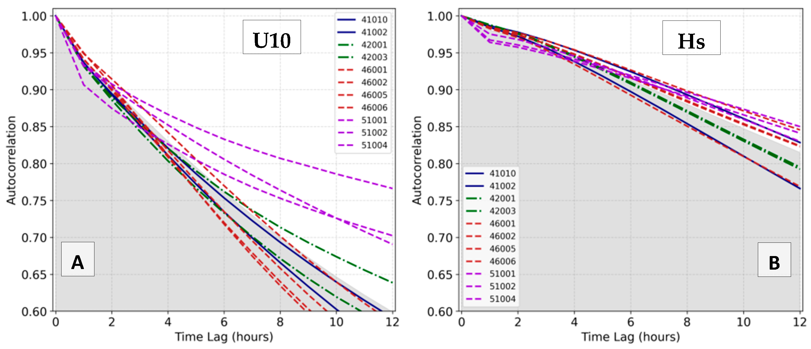
The autocorrelation function is an excellent means of analyzing the impact of time lags on correlation coefficients. Figure 2 displays the autocorrelation curves for each buoy, examining time displacements up to 12 h. The rapid decay in correlation, particularly for U10, suggests that the temporal criteria should be more stringent for U10 than for Hs. This also indicates that metocean prediction is typically more challenging for U10 than for Hs, as there is more short-term variation in wind speed than in wave height. Regarding Hs, correlation values above 0.95 are observed within the first 3 h, whereas for U10, the same value of 0.95 is reached within 1 h, confirming the widely used time resolution of output files from numerical prediction systems, which is typically 1 h for wind speed and 3 h for wave heights. In other words, providing hourly information for forecast users is crucial when dealing with U10, while 3 h would suffice for Hs. Furthermore, correlations for Hs drop below 0.90 only after 6 h, providing valuable information for the validation of wave forecasts; i.e., if the 6 h forecast has a correlation coefficient lower than 0.90, then using the current wave observation as a 6 h forecast would provide better information (in terms of correlation coefficient only).
In Figure 2, it is interesting to note the differences between the buoys. After a 3 h time lag, the buoys in the Tropical Pacific Ocean (Hawaii) exhibit higher correlations compared to the other stations, while the buoys in the Extra-tropical Pacific Ocean (northwestern coasts of the USA), at higher latitudes, display lower values, particularly for U10. Moreover, Figure 2 illustrates that the differences among buoys are larger for U10 than for Hs. At a 12 h time lag, the average autocorrelation for U10 drops to 0.60, while for Hs, it is 0.82, demonstrating how wave fields function as low-pass filters of the surface wind fields.
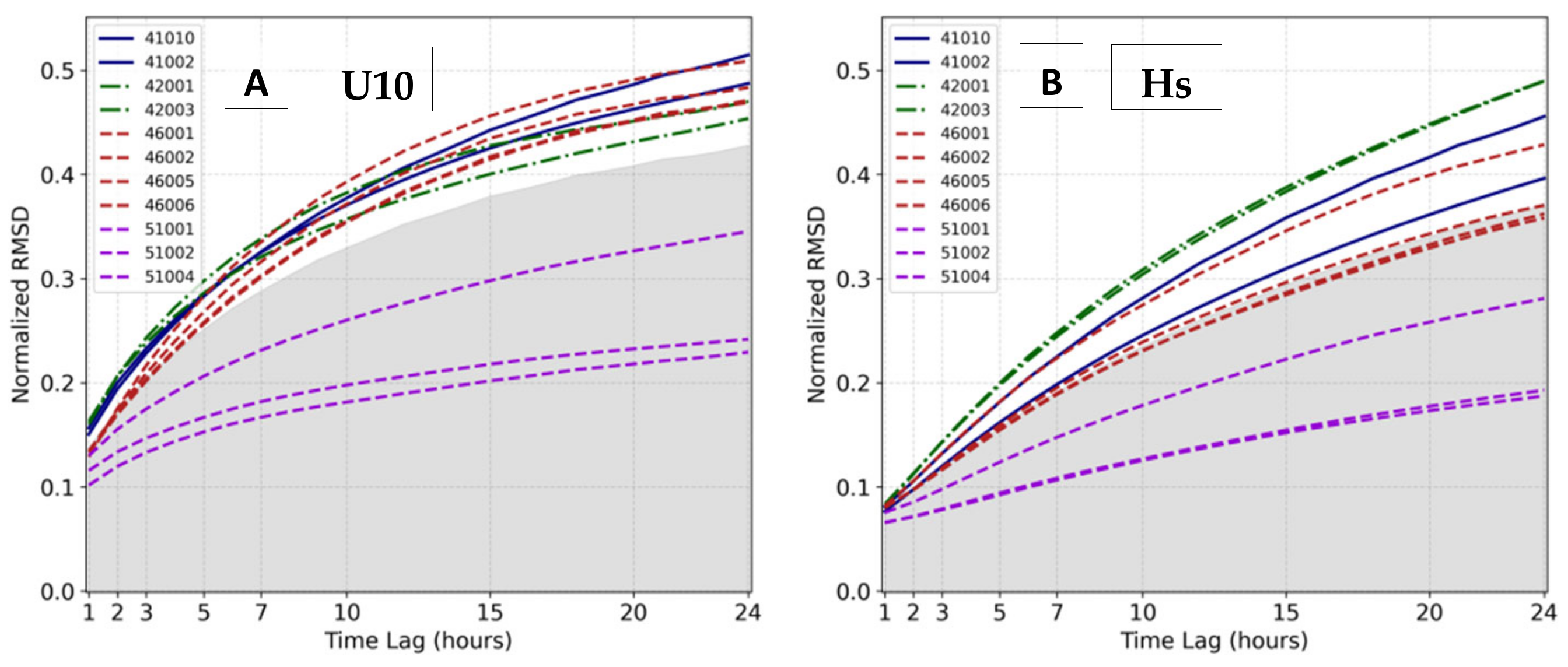
The increase in normalized root mean square differences as a function of the time lag is depicted in Figure 3, which extends to 24 h. As a normalized metric, it can be interpreted as a percentage measure of RMSD when multiplied by 100. Consistent with Figure 2, the normalized RMSD shows a more rapid increase for U10 than for Hs, particularly in the first 12 h. When comparing the buoys, the RMSD is lower for the Tropical Pacific Ocean buoys, which aligns with the higher autocorrelations in Figure 2. On the other hand, for Hs, the RMSD is higher in the Gulf of Mexico than the other clusters. In terms of values, the two plots of Figure 3 illustrate a fast increase in RMS differences when displacing a few hours, reaching an average of 20% of differences in 3 h for U10 and 7 h for Hs. For 1 h only, it starts with 12% for U10 and 8% for Hs.
Table 2 summarizes the discussion so far, presenting the RMSD, SI, and CC for time lags ranging from 1 to 12 h. For the first hour (1 h time lag), the RMSD of Hs is already very close to the accuracy of the wave buoy, which is equal to 0.2 m according to the NDBC [38], and it is very similar to the RMSE of calibrated forecast products using WAVEWATCH III, which ranges from 0.2 to 0.5 m according to [36,69,70]. This is also valid for U10, where the 1 h time lag is even higher than the NDBC accuracy of 0.55 m/s.
The effect of time lag on the scatter error is also notable in Table 2, with values exceeding 10% in 3 h for Hs and only 1 h for U10. The results of Figure 1 and Figure 2 and Table 2 are in agreement with Monaldo [28], who used one month of buoy observations in November 1985. He found the RMSD reached 0.5 m with an approximate time lag of 4 h, while Table 2 shows a lag of 6 h on average—the variation among buoys must be considered. The decay of CC values is 0.96 for a 3 h time lag for Hs and 0.87 for U10. This significant impact of time displacement on the statistics indicates rapid changes in wind and wave conditions in a short period of time.
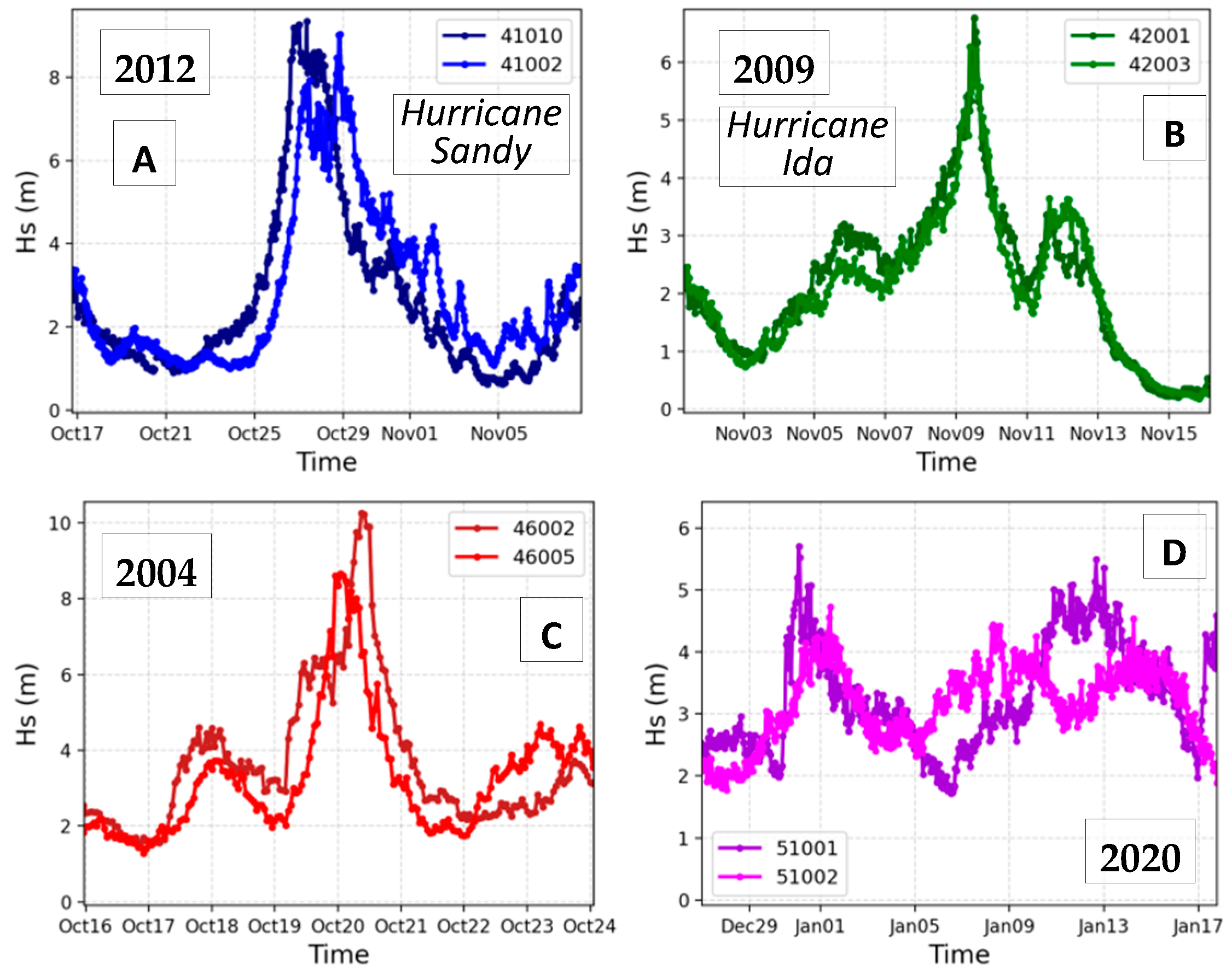
In order to briefly explore the variations in Hs and U10 with time, Figure 4 and Figure 5 were generated, including the variance spectrum [71] and time-series plots, to illustrate some events. Figure 4 suggests that the main changes in the wind and wave conditions do not necessarily occur in a few hours but beyond 24 h of time, responding to large-scale meteorological systems. The daily cycle is more evident in U10 than Hs, and the most significant modifications in the metocean conditions occur at 48 h and beyond. This finding may contradict the discussion above (Figure 2 and Figure 3 and Table 2); however, despite the great influence of synoptic systems, there is still a secondary high-frequency effect embedded in the variance that can be visualized in Figure 5. Although the events illustrated last two days or more, the evolution of Hs time shows short rises and falls that can reach more than one meter in one hour, including occasional periods with approximately 15% of hourly variations embedded in the low-frequency component. Since this type of short fluctuation is occasional, apparently random, varies in amplitude, and lacks a constant pattern, it is not highlighted in the variance spectrum.
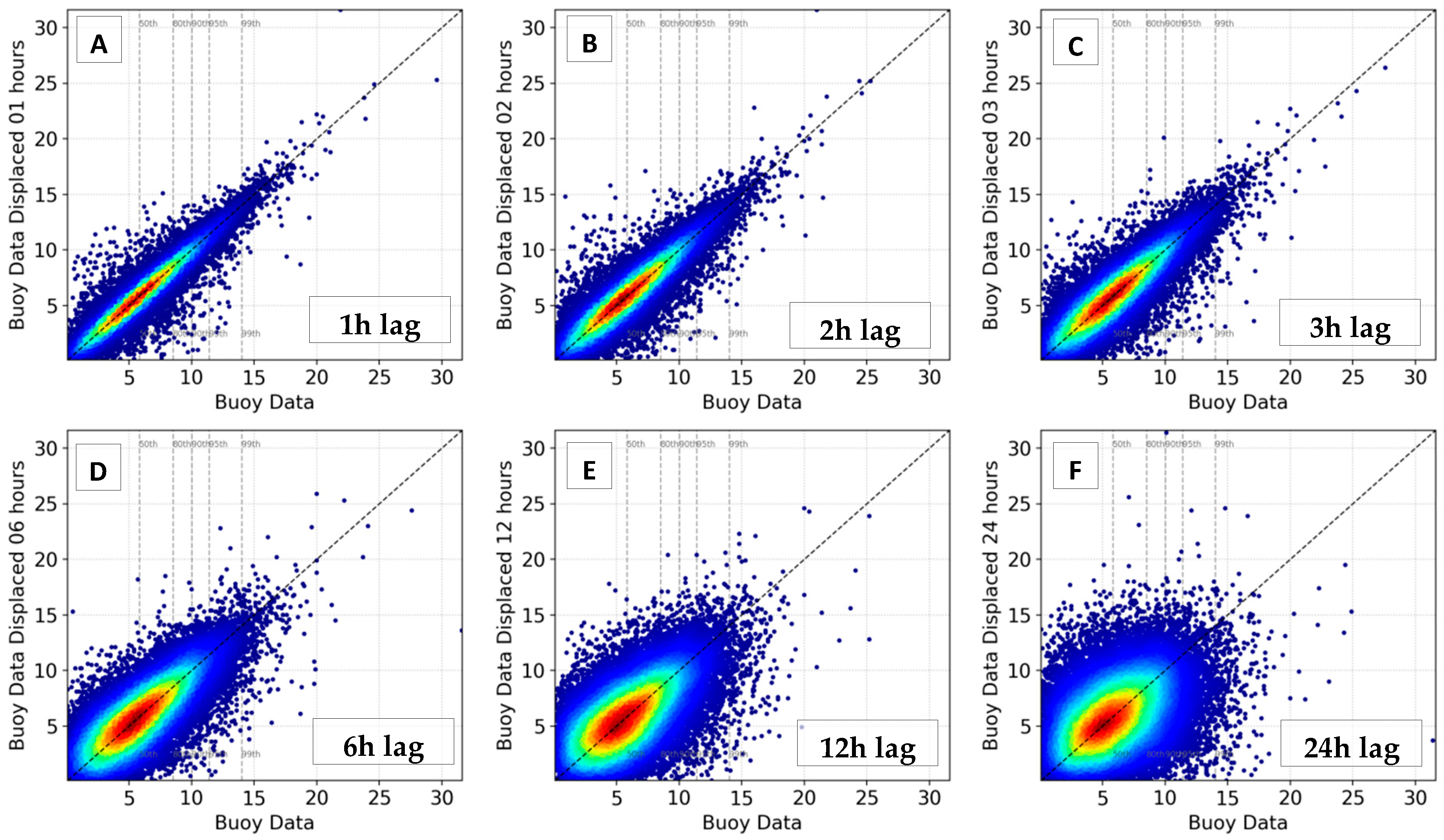
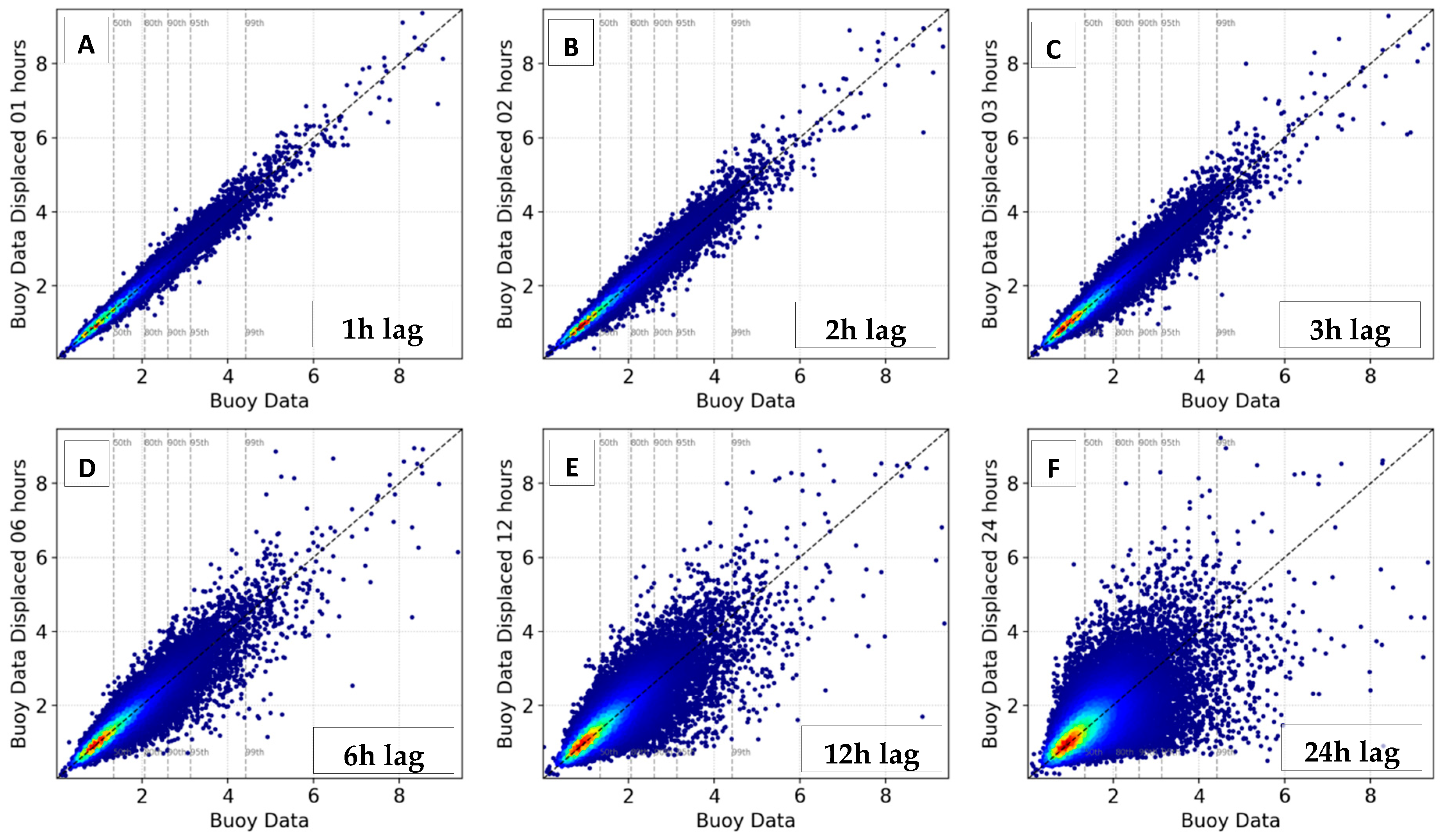
It is important to note that Figure 2, Figure 3 and Figure 4 provide bulk metrics or average patterns. However, specific conditions and events may cause significant variations in autocorrelation and RMSD, which should be considered when establishing criteria. Scatter plots are a better way to visualize the time lag in this case, and this approach has been extensively explored by many authors in this type of study (e.g., [53]). Figure 6 and Figure 7 show scatter plots of U10 and Hs with time lags ranging from 1 h to 24 h. They clearly demonstrate a much larger spread of U10 compared to Hs. The hot colors in the plots indicate the highest density, but it is also important to analyze the overall distribution of points and the largest differences observed.
The scatter plots of Hs (Figure 7) show very small differences between time-series with time lags of up to three hours, although the larger waves for the 3 h time lag display some concerning discrepancies. Regarding U10 (Figure 6), the first plot with a 1 h time lag already exhibits significant scattering. Therefore, a temporal criterion above one hour is not recommended.
In summary, the analyses suggest that temporal criteria of 1 or 2 h would be appropriate for Hs, while 1 h or less would be recommended for U10, although this may vary depending on the location (four locations addressed) and conditions (points of scatter plots). Since it is challenging to define different temporal collocation criteria for Hs and U10 that vary with time and location, a conservative compromise can be achieved by using a maximum of 1 h for the temporal distance between records to be averaged. In practical terms, a limit of 1800 s (plus and minus) centered at the hourly buoy time defines a suitable temporal criterion for altimeter collocation, which is consistent with the fundamental studies of Monaldo [28] and Ribal and Young [23].

3.2. Spatial Analysis Using Altimeter Data

The spatial analysis started by applying temporal criteria, which involved selecting altimeter records where the overpass occurred within 30 min of the hourly buoy data. This was followed by the methodology steps outlined in Section 2.3, where track sections passing very close to the buoys positions were selected. The next figures are based on Hs and U10 AODN altimeter data without any calibration. Later, in Section 3.3, the calibration proposed by Ribal and Young [23] is evaluated.
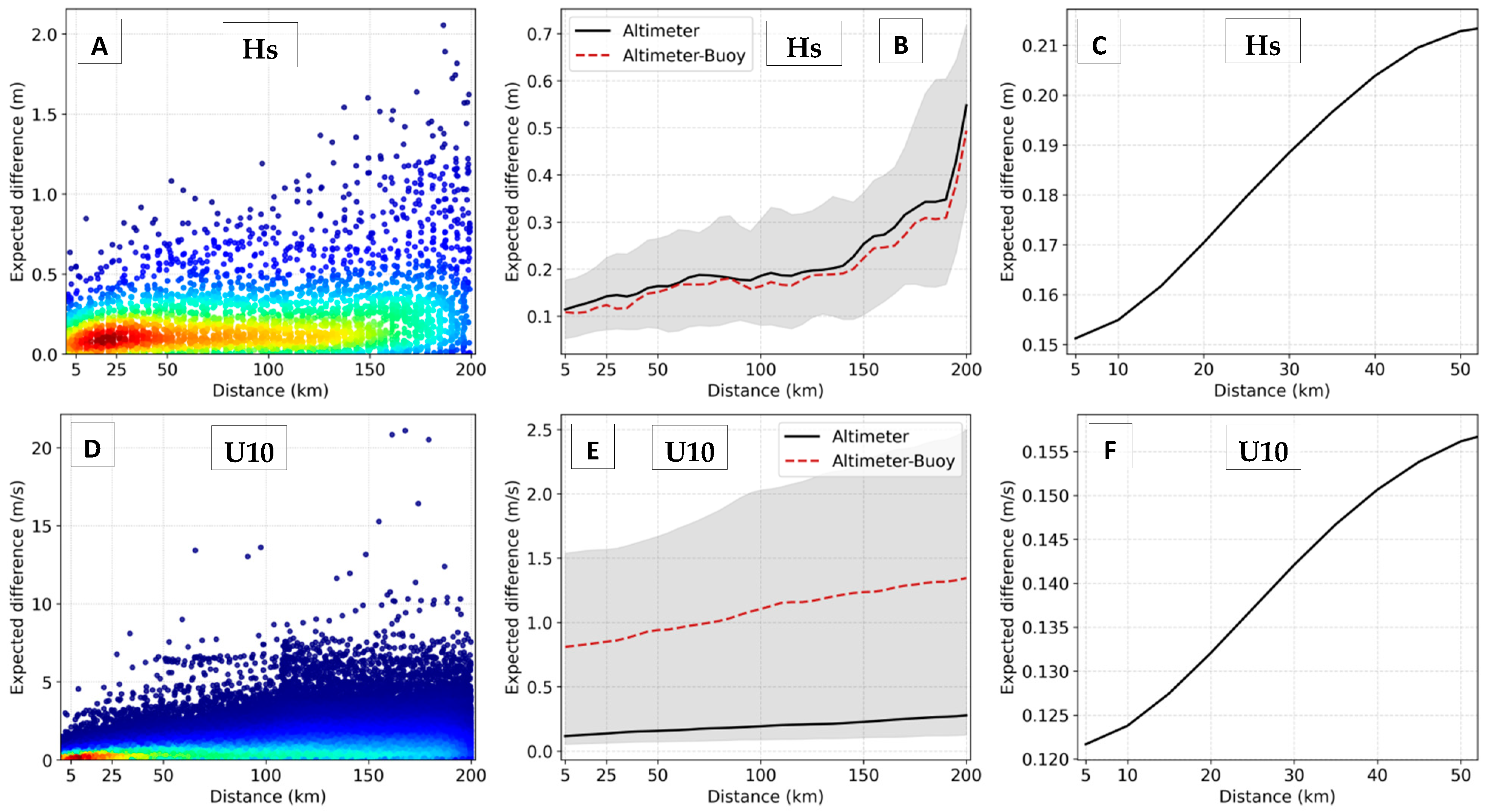
Figure 8 provides a vast amount of information regarding altimeter–altimeter and altimeter–buoy comparisons. Figure 8A,D show scatter plots of altimeter measurements compared to the single closest altimeter record to the buoy’s position for each satellite track passage—presented as the “expected difference” in the plots, a term used by Monaldo [28]. The scatter plots show a growing spread as the distance increases, especially beyond 100 km. The density at lower expected difference values is higher at distances between 5 to 50 km. Conversely, small distances also present some points with large differences, while large distances also contain pairs with small differences. However, the general pattern indicates the best agreement within the first 50 km. This can be confirmed by counting the number of points with differences above 1 m in Figure 8A. Therefore, the scatter plots provide a first indication of suitable spatial criteria that should be restricted to the first 50 km.
Figure 8B confirms the large discrepancies for altimeter records more than 100 km apart. The plot also provides the first indication of good agreement between altimeter and buoy data in terms of Hs, with the black solid curve being very close to the dashed red curve. This result is not replicated in Figure 8E for U10, where the differences between altimeter and buoy data are much larger than for Hs, highlighting the importance of altimeter wind calibration described in Ribal and Young [23]. The spread of expected differences for U10 (Figure 8D,E) is also very high, but it is reduced within the first 25 km, which can be observed by counting the number of points above 5 m/s in Figure 8D.
A clearer representation of the average increase in mean differences within the first 50 km is presented in Figure 8C,F. The curve for Hs crosses the 0.20 m value (a level associated with buoy accuracy according to the NDBC and linked to high-quality simulations using WAVEWATCH III) at approximately 37 km. It reaches a mean difference of 0.21 m at the 50 km distance, which is small in terms of mean difference, but at 20 km, it is only 0.17 m. The latter represents a sampling variability with low RMS difference that has the potential to benefit the validation and analysis of highly accurate products. The same curve for U10 (Figure 8F) shows much lower values for mean differences associated with spatial displacement, despite the large spread and occasional large differences encountered in Figure 8D. This means that the arithmetic mean can successfully filter out those less frequent large discrepancies, once again demonstrating the benefits of space–time averages for altimeter collocation instead of selecting the single closest altimeter record.
The current results show lower differences as a function of distance than those reported by [28]. Monaldo [28] found differences of 0.5 m at 100 km and 0.2 m at 20 km, while Figure 8 shows the 0.2 m level being crossed at 37 km. It should be noted that Monaldo’s [28] observations were based on GEOSAT altimeter data, while Figure 8 was calculated using 3133 records from JASON3. Hwang et al. [67] found that when spatial lags are less than 10 km, the differences in Hs are approximately 0.1 m, which is more similar to what has been reported so far, around 0.15 m. It is worth remembering that these differences are among individual satellite records or direct comparisons against buoy data and do not necessarily represent the result found after collocation, which involves computing the average of all altimeter records inside a circle to yield a single value (mean) per transect. In other words, the spatial separation criterion defines a circle of diameter in which satellite data are selected, so an altimeter transect that passes directly over the buoy will have a transect length of 100 km when the traditional 50 km criterion is utilized. More distant passes will define shorter chords of the circle. Each transect within the circle will only define one collocated value of Hs and U10, reducing the data size.
As described earlier, the analysis in this section only considers altimeter transects in which at least one record is very close to the buoy, within 10 km. Figure 9 shows the number of JASON3 altimeter records selected for different spatial criteria, ranging from 10 to 200 km. Considering that the distance of consecutive JASON3 measurements is 5.87 km, it is expected that a 10 km radius (20 km diameter) will select only two or three altimeter records. Moving to a 25 km radius increases the average number of records to eight, which is above the minimum number of five points discussed in Ribal and Young [23], and eight is the default number of neighbors used in python pyresample kd_tree. The commonly used 50 km criterion selects around 15 records, while 100 km and 200 km criteria select, on average, 30 and 60 records, respectively. Therefore, the large RMS differences at larger distances must be balanced with the number of points to be averaged in order to avoid using an overly restrictive criterion, such as 10 km, which would provide an insufficient number of records for a proper final estimate.
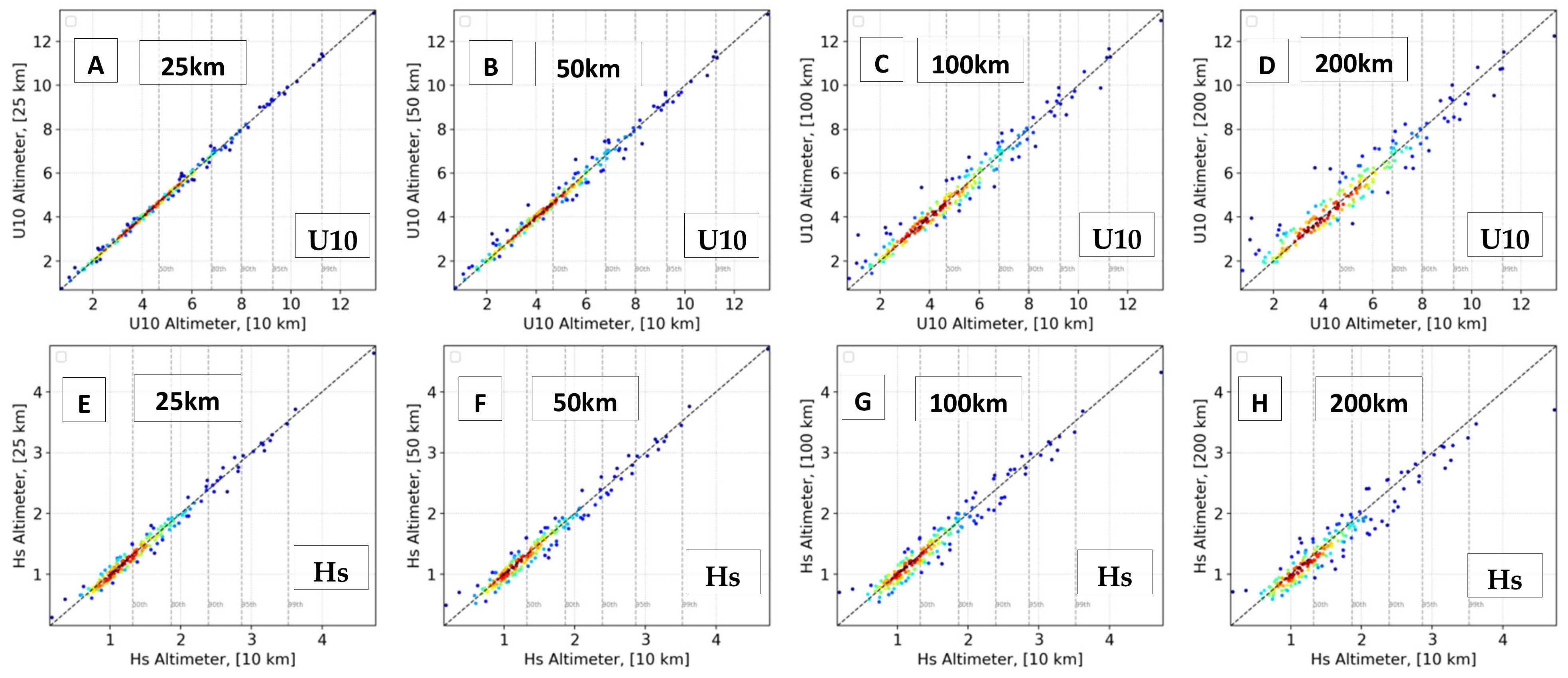
A new comparison and assessment must be re-run at this point, using transect averaging results for different criteria as a sensitivity analysis of the spatial criterion. Figure 10 presents the scatter plots comparing the effect of different spatial criterion on the collocated satellite data. It is interesting to note the lower scattering, with points falling close to the main diagonal, when compared to Figure 6 and Figure 7, associated with non-averaged measures. This once again emphasizes the benefits of the averaging process. The results for 10 km, 25 km, and 50 km are very similar, with an increasing spread associated with 100 km and 200 km radii. The upper points representing the most severe intensities start to diverge to the main diagonal only in the 100 km and 200 km plots. Therefore, Figure 10 proves the stability and robustness of the collocation using the spatial mean, especially for radii of 25 and 50 km. The problem of extremely large scattering of U10 (Figure 6) has been solved by using spatial averaging, making the methodology even more relevant when wind speeds are included. In this section, the estimates calculated using the spatial criterion of 10 km were used as a reference. The next section will select the buoy data for that purpose.
Statistical metrics (Equations (2)–(5)) were calculated to further investigate the influence of the spatial criteria on the final estimates of Hs and U10. Figure 11 presents the scatter and systematic differences together. It is possible to see a very close agreement between results using the spatial criteria of 10 to 50 km, followed by a progressive divergence for 100 km, and magnified discrepancies for 200 km—in both error metrics. Within 50 km, the scatter differences remain below 10% and the systematic differences below 1% for both U10 and Hs.
Table 3 provides statistical results for four metrics (Equations (2)–(5)) that further complement Figure 11. The bias is very low for both Hs and U10, even at greater radii. Thus, the main impact of increasing the spatial averaging radius r is on the increase in scatter errors (with a consequent increase in the RMSD) and decrease in the correlation coefficient. The scatter differences are above 10% for r equal to and above 50 km for Hs and 200 km for U10. Figure 10 and Figure 11 and Table 3 show the significant effect of spatial averaging on the collocation of Hs and U10 when compared to Figure 8, which contains the original altimeter records. Using the altimeter tracks as shown in Figure 8 may lead to occasional very discrepant values and strong deterioration when considering further distances. However, when the spatial mean is applied, it smooths out the discrepant values, providing more stable estimates with low scatter differences and better results at larger radii. Even so, the results from Figure 10 and Figure 11 and Table 3 still indicate that the upper limit of 50 km is a suitable spatial criterion for altimeter collocation. However, the results so far are related to altimeter–altimeter comparison and not direct validation against buoy measurements, which is essential to consider and is performed in the next section.

3.3. Spatial Averaging Method and Altimeter Validation

In this section, the altimeter dataset is expanded from JASON3 only to JASON3, JASON2, CRYOSAT2, JASON1, HY2, SARAL, and SENTINEL3A. These satellite missions have high accuracies and demonstrate close agreement in the cross-validations performed by Ribal and Young [23], providing a vast dataset of reliable information from altimeters. Additionally, the AODN-calibrated variables of Hs and U10, namely Hsc and U10c, were also included. The temporal criterion r = 1800 s was first applied, and two spatial criteria of τ = 25 and 50 km were tested. The methodology was the same as the previous section, but the comparisons were now performed against buoy data. Apart from the arithmetic ensemble mean, two other averaging methods were included: (i) the inverse distance weighting, using a simple linear function (named LIDW); and (ii) the same inverse distance weighting, but a Gaussian function was applied instead of a linear decay (named GF). The inverse distance weighting method has a very intuitive assumption that the closer a point is to the center position being estimated, the more influence or weight it has in the averaging process. The calculation was performed using the python package pyresample.kd_tree.
Table 4 and Table 5 present the final assessment, where the poorest results are highlighted in red, and the best results are highlighted in green. Initially, it is clear that using a single nearest altimeter record to the buoy measurement does not provide optimal estimates compared to using the spatio-temporal averaging of altimeter records. The worst performances are confirmed through high impacts on RMSE, SI, and CC. This characteristic is more evident for Hs than U10. Next, the comparison between the three averaging methods shows very similar results, with minor differences in the third decimal of the error metrics. It is inconclusive at this stage. Thus, the simple arithmetic mean, which is widely used, remains a good option, at least for the dataset and validation considered in this study.
The most notable impact, leading to a great improvement in the error metrics, is found in the calibrated variables, Hsc and U10c. The AODN calibration [23] resulted in a reduction in Bias, RMSE, and SI, combined with an increase in CC. This effect is more pronounced for wind speed, where the RMSE of U10 of 2.02 m/s (τ = 50 km, from arithmetic mean) was reduced to 1.68 m/s for U10c. For the same comparison, the CC improved from 0.79 to 0.89. However, the bias shifted from −0.49 m/s (underestimation of altimeter winds) to 0.76 m/s (overestimation of altimeter winds), which warrants further investigation.
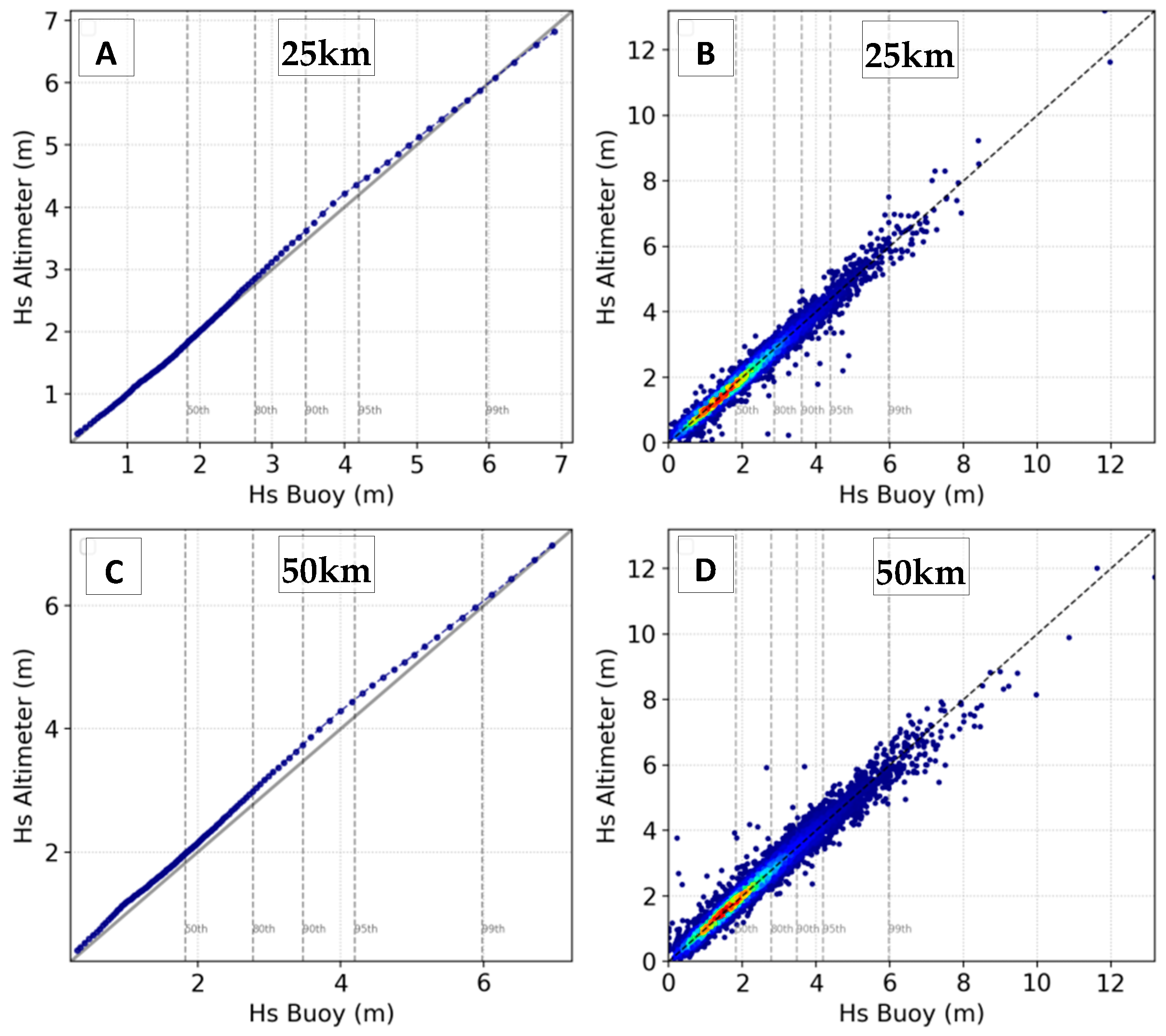
The best performance in Table 4 and Table 5 is observed in Hsc, where the calibration succeeded in improving all four metrics, and the results exhibit almost no bias (around 1 cm only). The RMSE of Hsc is 0.21 m, the scatter errors are at 9%, and the correlation coefficient is 0.98. Figure 12 presents the results for Hsc and confirms the excellent performance of collocated altimeter data shown in Table 4. The Hsc quantiles closely follow the main diagonal of QQ-plots, and the scatter plots also show the points not far from the diagonal of perfect agreement, ranging from small values to the highest ones above the 99th percentile.

4. Discussion

The results presented in Section 3.1, Section 3.2 and Section 3.3 have allowed for the narrowing down of options for spatial and temporal criteria for altimeter collocation to fixed-point positions. In addition to the expected differences and increasing errors due to time and distance previously discussed, two other aspects should be considered: (i) the number of records for each altimeter transect within a defined diameter to be averaged, which is shown in Figure 9 and briefly discussed above, and (ii) the final number of collocated matchups of altimeter/buoy resulting from the combination of each temporal and spatial criterion. Table 6 provides an example of the total resulting collocated data of JASON3 altimeter data at 11 buoy positions as a function of temporal and spatial criteria. The variation in the number of matchups is significant, ranging from as few as 294 for r , τ equal to 10 km and 15 min, to 50.6 thousand for r , τ of 100 km and 2 h. The widely used criteria of 30 min and 50 km led to 3.7 thousand matchups of JASON3 at the 11 points.
Depending on the practical application of collocated altimeter data, there may be an urgent need to expand the dataset by increasing the number of matchups through the spatial and temporal criteria. For example, this may be necessary when more observations are required for an important event and case study, or for extreme value analyses where data length impacts the reliability of extrapolations. On the other hand, when long time analyses are conducted and the accuracy of collocated satellite is critical, then smaller criteria of τ and r can be considered. However, in practical terms, the options for adapting τ and r to specific needs are limited due to the important points:
(1) Small spatial criterion r results in lower RMS differences but reduces the number of records for the circle average, potentially selecting only one record, which is equivalent to using the single closest altimeter measurement to the buoy’s position. Ribal and Young [23] recommend a minimum of five altimeter records for the average, which is achievable for r typically above 20 km, thus discarding the r = 10 km option evaluated in this paper.
(2) A temporal criterion (τ) below 1800 s results in a small number of matchups (Table 6), which limits the practical use of altimeter data. Monaldo [28] suggests that approximately 1000 altimeter–buoy comparison pairs are required to validate altimeter performance and distinguish between competing wind speed algorithms.
(3) Increasing the temporal criterion τ to values above 1800 s compromises the RMSE of the final estimates, as shown in Section 3.1. The effect of a 1 h time lag on the final error is close to the NDBC and altimeter intrinsic errors [38] and just below the accuracies of calibrated wave forecast products using WAVEWATCH III [36,69,70]. For U10, the temporal criterion τ is even more critical, anchoring the ideal temporal criterion to 1800 s.
(4) The spatial analysis indicates that the density at lower expected difference values is higher at distances between 5 and 50 km (Figure 8A,D). The curve of Hs RMSD as a function of distance (Figure 8C) reaches a mean difference of 0.21 m at 50 km. Therefore, Section 3.2 clearly shows that extrapolating to a spatial criterion   r greater than 50 km is not recommended.
In summary, a temporal criterion of τ = 1800 s and spatial criteria of r between 25 to 50 km are the best options for collocating altimeter data to fixed point positions. Table 4 and Table 5 confirm the success of these values. The resulting differences between collocated altimeter data and buoy observations, using AODN-calibrated data of Hs and U10, are smaller than those reported by [20,23,25] and in line with the findings of Ribal and Young [23].
The results presented so far have been obtained from 11 deep-water points. For those interested in coastal areas or very extreme events (especially tropical cyclones), a separate analysis must be conducted with more buoys, a larger dataset, and IBTrACS cyclone tracks.

5. Conclusions

This paper investigated the spatial and temporal sampling variability and the differences between altimeter and buoy data. In practical terms, an important question arises: is the widely used criteria of 30 min and 50 km, which has been established for more than 30 years, still a good option for altimeter collocation in deep waters? The overall answer is yes. A small margin for variation on the spatial criterion r is open between 25 and 50 km, as shown in Table 4 and Table 5 and Figure 12. The lower bound of 25 km leads to slightly better error metrics but with the cost of fewer collocated matchups (Table 6). The 50 km criterion maximizes the resulting collocated data size while keeping the differences to buoy measurements very low. Young et al. [34] argue that the criteria of r = 50 km and τ = 30 min produce a sufficient number of collocations for a stable result while ensuring that both buoy and altimeter respond to the same approximate wind and wave field.
Additionally, it is possible to conclude that using the single closest altimeter record to the buoy position leads to worse results compared to the collocation method based on temporal and spatial averaging (Table 4 and Table 5). Regarding the averaging method, very small differences were encountered between the simple arithmetic mean and the inverse distance weighting. The validation of altimeter collocated data against 11 NDBC buoys proves the quality of the AODN calibrated dataset [23] combined with the collocation method and criteria analyzed here. The RMSD of 0.21 m, scatter index of 0.09, and correlation coefficient of 0.98 for Hsc confirm the success of the methodology and altimeter data employed, supporting future studies demanding high-quality and reliable altimeter observations.

Funding

This work was funded by the Cooperative Institute for Marine and Atmospheric Studies (CIMAS), a Cooperative Institute of the University of Miami and the National Oceanic and Atmospheric Administration, cooperative Agreement NA20OAR4320472.

Data Availability Statement

NOAA National Data Buoy Center historical data: https://www.ndbc.noaa.gov/historical_data.shtml (accessed on 1 July 2022); AODN altimeter database: http://thredds.aodn.org.au/thredds/catalog/IMOS/SRS/Surface-Waves/Wave-Wind-Altimetry-DM00/catalog.html (accessed on 1 July 2022); ETOPO1/NOAA bathymetry: https://www.ngdc.noaa.gov/mgg/global/global.html (accessed on 1 July 2022); GSFC/NASA distance to coast: https://oceancolor.gsfc.nasa.gov/docs/distfromcoast/ (accessed on 1 July 2022).

Acknowledgments

The author would like to acknowledge the supervision, scientific discussions, and technical support provided by Darin Figurskey, Avichal Merha, Ali Abdolali, Jessica Meixner, and Matthew Masarik. Additionally, it is important to acknowledge the significant effort of NOAA/NDBC and IMOS/AODN in providing publicly available, high-quality buoy and altimeter datasets.

Conflicts of Interest

The author declares no conflict of interest.

References

  1. Wimmer, W.; Challenor, P.; Retzler, C. Extreme wave heights in the North Atlantic from Altimeter Data. Renew. Energy 2006, 31, 241–248. [Google Scholar] [CrossRef]
  2. Alves, J.H.G.M.; Young, I.R. On estimating extreme wave heights using combined Geosat, Topex/Poseidon and ERS-1 altimeter data. Appl. Ocean Res. 2004, 25, 167–186. [Google Scholar] [CrossRef]
  3. Ozbahceci, B.O. Extreme value statistics of wind speed and wave height of the Marmara Sea based on combined radar altimeter data. Adv. Space Res. 2020, 66, 2302–2318. [Google Scholar] [CrossRef]
  4. Young, I.R.; Zieger, S.; Babanin, A.V. Global trends in wind speed and wave height. Science 2011, 332, 451–455. [Google Scholar] [CrossRef]
  5. Hochet, A.; Dodet, G.; Ardhuin, F.; Hemer, M.; Young, I.R. Sea State Decadal Variability in the North Atlantic: A Review. Climate 2021, 9, 173. [Google Scholar] [CrossRef]
  6. Stopa, J.E. Seasonality of wind speeds and wave heights from 30 years of satellite altimetry. Adv. Space Res. 2021, 68, 787–801. [Google Scholar] [CrossRef]
  7. Young, I.R.; Ribal, A. Can Multi-Mission Altimeter Datasets Accurately Measure Long-Term Trends in Wave Height? Remote Sens. 2022, 14, 974. [Google Scholar] [CrossRef]
  8. Erikson, L.; Morim, J.; Hemer, M.; Young, I.R.; Wang, X.L.; Mentaschi, L.; Mori, N.; Semedo, A.; Stopa, J.; Grigorieva, V.; et al. Global ocean wave fields show consistent regional trends between 1980 and 2014 in a multi-product ensemble. Commun. Earth Environ. 2022, 3, 320. [Google Scholar] [CrossRef]
  9. Stopa, J.E.; Cheung, K.F. Intercomparison of wind and wave data from the ECMWF Reanalysis Interim and the NCEP Climate Forecast System Reanalysis. Ocean Model. 2014, 75, 65–83. [Google Scholar] [CrossRef]
  10. Shi, J.; Zheng, J.; Zhang, C.; Joly, A.; Zhang, W.; Xu, P.; Sui, T.; Chen, T. A 39-year high resolution wave hindcast for the Chinese coast: Model validation and wave climate analysis. Ocean Eng. 2019, 183, 224–235. [Google Scholar] [CrossRef]
  11. Campos, R.M.; Gramcianinov, C.B.; Camargo, R.; Dias, P.L.S. Assessment and Calibration of ERA5 Severe Winds in the Atlantic Ocean Using Satellite Data. Remote Sens. 2022, 14, 4918. [Google Scholar] [CrossRef]
  12. Janssen, P.A.E.M.; Hansen, B.; Bidlot, J.-R. Verification of the ECMWF Wave Forecasting System against Buoy and Altimeter Data. Weather Forecast. 1997, 12, 763–784. [Google Scholar] [CrossRef]
  13. Campos, R.M.; Alves, J.H.G.M.; Penny, S.G.; Krasnopolsky, V. Global assessments of the NCEP Ensemble Forecast System using altimeter data. Ocean Dynam. 2020, 70, 405–419. [Google Scholar] [CrossRef]
  14. Campos, R.M.; Bernardino, M.; Gonçalves, M.; Guedes Soares, C. Assessment of metocean forecasts for Hurricane Lorenzo in the Azores Archipelago. Ocean Eng. 2022, 243, 110292. [Google Scholar] [CrossRef]
  15. Esteva, D.C. Evaluation of preliminary experiments assimilating Seasat significant wave heights into a spectral wave model. J. Geophys. Res. 1988, 93, 14099–14105. [Google Scholar] [CrossRef]
  16. Young, I.R.; Glowacki, T.J. Assimilation of altimeter wave height data into a spectral wave model using statistical interpolation. Ocean Eng. 1996, 23, 667–689. [Google Scholar] [CrossRef]
  17. Yu, H.; Li, J.; Wu, K.; Wang, Z.; Yu, H.; Zhang, S.; Hou, Y.; Kelly, R.M. A global high-resolution ocean wave model improved by assimilating the satellite altimeter significant wave height. Int. J. Appl. Earth Obs. Geoinf. 2018, 70, 43–50. [Google Scholar] [CrossRef]
  18. Toledano, C.; Ghantous, M.; Lorente, P.; Dalphinet, A.; Aouf, L.; Sotillo, M.G. Impacts of an Altimetric Wave Data Assimilation Scheme and Currents-Wave Coupling in an Operational Wave System: The New Copernicus Marine IBI Wave Forecast Service. J. Mar. Sci. Eng. 2022, 10, 457. [Google Scholar] [CrossRef]
  19. Campos, R.M.; Krasnopolsky, V.; Alves, J.-H.; Penny, S.G. Improving NCEP’s global-scale wave ensemble averages using neural networks. Ocean Model. 2020, 149, 101617. [Google Scholar] [CrossRef]
  20. Dobson, E.; Monaldo, F.; Goldhirsh, J.; Wilkerson, J. Validation of Geosat altimeter-derived wind speeds and significant wave heights using buoy data. J. Geophys. Res. 1987, 92, 10719–10731. [Google Scholar] [CrossRef]
  21. Durrant, T.H.; Greenslade, D.J.M.; Simmonds, I. Validation of Jason-1 and Envisat Remotely Sensed Wave Heights. J. Atmos. Ocean. Technol. 2009, 26, 123–134. [Google Scholar] [CrossRef]
  22. GlobWaveTeam. Deliverable D30. GlobWave Final Report. 2013. Available online: http://due.esrin.esa.int/page_project102.php (accessed on 1 July 2022).
  23. Ribal, A.; Young, I.R. 33 years of globally calibrated wave height and wind speed data based on altimeter observations. Sci. Data 2019, 6, 77. [Google Scholar] [CrossRef] [PubMed]
  24. Dodet, G.; Piolle, J.-F.; Quilfen, Y.; Abdalla, S.; Accensi, M.; Ardhuin, F.; Ash, E.; Bidlot, J.-R.; Gommenginger, C.; Marechal, G.; et al. The Sea State CCI dataset v1: Towards a sea state climate data record based on satellite observations. Earth Syst. Sci. Data 2020, 12, 1929–1951. [Google Scholar] [CrossRef]
  25. Zieger, S.; Vinoth, J.; Young, I.R. Joint calibration of multi-platform altimeter measurements of wind speed and wave height over the past 20 years. J. Atmos. Ocean. Tech. 2009, 26, 2549–2564. [Google Scholar] [CrossRef]
  26. Cooper, C.K.; Forristall, G.Z. The use of satellite altimeter data to estimate extreme wave climate. J. Atmosph. Oceanic Technol. 1997, 14, 254–266. [Google Scholar] [CrossRef]
  27. Jason-3 Products Handbook. 2018; CNES: SALP-MU-M-OP-16118-CN. Available online: https://www.ospo.noaa.gov/Products/documents/hdbk_j3.pdf (accessed on 1 July 2022).
  28. Monaldo, F. Expected differences between buoy and radar altimeter estimates of wind speed and significant wave height and their implications on buoy-altimeter comparisons. J. Geophys. Res. 1988, 93, 2285–2302. [Google Scholar] [CrossRef]
  29. Gower, J.F.R. Intercalibration of wave and wind data from TOPEX/POSEIDON and moored buoys off the west coast of Canada. J. Geophys. Res. 1996, 101, 3817–3829. [Google Scholar] [CrossRef]
  30. Young, I.R.; Holland, G.J. Atlas of the Oceans: Wind and Wave Climate; Pergamon Press: New York, NY, USA, 1996; p. 241. [Google Scholar]
  31. Queffeulou, P. Validation of ENVISAT RA-2 and JASON-1 altimeter wind and wave measurements. In Proceedings of the 2003 IEEE International Geoscience and Remote Sensing Symposium IGARSS, Toulouse, France, 21–25 July 2003; Volume 5, pp. 2987–2989. [Google Scholar] [CrossRef]
  32. Queffeulou, P. Long-term validation of wave height measurements from altimeters. Mar. Geod. 2004, 27, 495–510. [Google Scholar] [CrossRef]
  33. Queffeulou, P.; Bentamy, A.; Guyader, J. Satellite wave height validation over the Mediterranean Sea. In Proceedings of the 2004 Envisat & ERS Symposium, Salzburg, Austria, 6–10 September 2004; European Space Agency: Paris, France, 2004; p. 208.1. [Google Scholar]
  34. Young, I.R.; Sanina, E.; Babanin, A.V. Calibration and cross-validation of a global wind and wave database of altimeter, radiometer, and scatterometer measurements. J. Atmos. Ocean. Technol. 2017, 34, 1285–1306. [Google Scholar] [CrossRef]
  35. Young, I.R.; Donelan, M.A. On the determination of global ocean wind and wave climate from satellite observations. Remote Sens. Environ. 2018, 215, 228–241. [Google Scholar] [CrossRef]
  36. Campos, R.M.; D’Agostini, A.; França, B.R.L.; Damião, A.L.A.; Guedes Soares, C. Implementation of a multi-grid operational wave forecast in the South Atlantic Ocean. Ocean Eng. 2022, 243, 110173. [Google Scholar] [CrossRef]
  37. National Data Buoy Center. NDBC Web Data Guide. 2015; 14p. Available online: https://www.ndbc.noaa.gov/docs/ndbc_web_data_guide.pdf (accessed on 1 July 2022).
  38. NDBC Technical Document 09-02, Handbook of Automated Data Quality Control Checks and Procedures. 2009. Available online: https://www.ndbc.noaa.gov/NDBCHandbookofAutomatedDataQualityControl2009.pdf (accessed on 1 July 2022).
  39. Evans, D.; Conrad, C.L.; Paul, F.M. Handbook of Automated Data Quality Control Checks and Procedures of the National Data Buoy Center; Document 03–02; NOAA National Data Buoy Center Tech: Hancock County, MS, USA, 2003; 44p. [Google Scholar]
  40. Det Norske Veritas/DNV-RP-C205 Recommended Practice, Environmental Conditions and Environmental Loads, April. 2007. Available online: https://www.dnv.com/oilgas/download/dnv-rp-c205-environmental-conditions-and-environmental-loads.html (accessed on 1 July 2022).
  41. Hsu, S.A.; Meindl, E.A.; Gilhousen, D.B. Determining the power-law wind-profile exponent under near-neutral stability conditions at sea. J. Appl. Meteor. 1994, 33, 757–765. [Google Scholar] [CrossRef]
  42. Jung, C.; Schindler, D. The role of the power law exponent in wind energy assessment: A global analysis. Int. J. Energy Res. 2021, 45, 8484–8496. [Google Scholar] [CrossRef]
  43. Bowler, N.E. Explicitly accounting for observation error in categorical verification of forecasts. Mon. Weather Rev. 2006, 134, 1600–1606. [Google Scholar] [CrossRef]
  44. Liu, Q.; Lewis, T.; Zhang, Y.; Sheng, W. Performance assessment of wave measurements of wave buoys. Int. J. Mar. Energy 2015, 12, 63–76. [Google Scholar] [CrossRef]
  45. Lawrence, J.; Coauthors, D. 2.1 Wave Instrumentation Database. Work Package 2: Standards and Best Practice. Revision: 05. 2012 Marine Renewables Infrastructure Network, European Union Seventh Framework Programme. 2012, 55p. Available online: https://www.marinet2.eu/wp-content/uploads/2017/04/D2.01-Wave-Instrumentation-Database.pdf (accessed on 1 July 2022).
  46. Ashton, I.G.C.; Johanning, L. On errors in low frequency wave measurements from wave buoys. Ocean Eng. 2015, 95, 11–22. [Google Scholar] [CrossRef]
  47. Bender, L.C.; Guinasso, N.L., Jr.; Walpertert, J.R.; Howden, S.D. A comparison of methods for determining significant wave heights—Applied to a 3-m discus buoy during Hurricane Katrina. J. Atmos. Ocean. Technol. 2010, 27, 1012–1028. [Google Scholar] [CrossRef]
  48. Donelan, M.; Pierson, W.J. The sampling variability of estimates of spectra of wind-generated gravity waves. J. Geophys. Res. 1983, 88, 4381–4392. [Google Scholar] [CrossRef]
  49. Thomas, J. Wave data analysis and quality control challenges. In Proceedings of the Oceans 2016 MTS/IEEE Monterey, Monterey, CA, USA, 19–23 September 2016. [Google Scholar] [CrossRef]
  50. Feng, H.; Vandemark, D.; Quilfen, Y.; Chapron, B.; Beckley, B. Assessment of wind-forcing impact on a global wind-wave model using the TOPEX altimeter. Ocean Eng. 2006, 33, 1431–1461. [Google Scholar] [CrossRef]
  51. Young, I.R.; Vinoth, J. An “extended fetch” model for the spatial distribution of tropical cyclone wind–waves as observed by altimeter. Ocean Eng. 2013, 70, 14–24. [Google Scholar] [CrossRef]
  52. Cotton, P.D.; Carter, D.J.T. Cross calibration of TOPEX, ERS-1, and Geosat wave heights. J. Geophys. Res. 1994, 99, 25025–25033. [Google Scholar] [CrossRef]
  53. Young, I.R. An intercomparison of GEOSAT, TOPEX and ERS1 measurements of wind speed and wave height. Ocean Eng. 1999, 26, 67–81. [Google Scholar] [CrossRef]
  54. Cancet, M.; Bijac, S.; Chimot, J.; Bonnefond, P.; Jeansou, E.; Laurain, O.; Lyard, F.; Bronner, E.; Féménias, P. Regional in situ validation of satellite altimeters: Calibration and cross-calibration results at the Corsican sites. Adv. Space Res. 2013, 51, 1400–1417. [Google Scholar] [CrossRef]
  55. Bao, L.; Gao, P.; Peng, H.; Jia, Y.; Shum, C.K.; Lin, M.; Guo, Q. First accuracy assessment of the HY-2A altimeter sea surface height observations: Cross-calibration results. Adv. Space Res. 2015, 55, 90–105. [Google Scholar] [CrossRef]
  56. Abdalla, S.; Dinardo, S.; Benveniste, J.; Janssen, P.A.E.M. Assessment of CryoSat-2 SAR mode wind and wave data. Adv. Space Res. 2018, 62, 1421–1433. [Google Scholar] [CrossRef]
  57. Kong, Y.; Zhang, X.; Sheng, L.; Chen, B. Validation and application of multi-source altimeter wave data in China’s offshore areas. Acta Oceanol. Sin. 2016, 35, 86–96. [Google Scholar] [CrossRef]
  58. Sepulveda, H.H.; Queffeulou, P.; Ardhuin, F. Assessment of SARAL AltiKa wave height measurements relative to buoy, Jason-2 and Cryosat-2 data. Mar. Geod. 2015, 38, 449–465. [Google Scholar] [CrossRef]
  59. Queffeulou, P.; Croizé-Fillon, D. Global Altimeter SWH Data Set. Laboratoire d’Océanographie Physique et Spatiale IFREMER. 2017. Available online: ftp://ftp.ifremer.fr/ifremer/cersat/products/swath/altimeters/waves/documentation/altimeter_wave_merge__11.4.pdf (accessed on 1 July 2022).
  60. GLOBWAVE Product User Guide. GlobWave/DD/PUGIssue 1.0. SatOC, Ifremer, NOC, CLS. Report No.: 21891/08/I-EC. 2010. Available online: http://globwave.ifremer.fr/download/ (accessed on 1 July 2022).
  61. Takbash, A.; Young, I.R.; Breivik, Ø. Global Wind Speed and Wave Height Extremes Derived from Long-Duration Satellite Records. J. Clim. 2019, 32, 109–126. [Google Scholar] [CrossRef]
  62. Willmott, C.J.; Ackleson, S.G.; Davis, R.E.; Feddema, J.J.; Klink, K.M.; Legates, D.R.; O’Donnell, J.; Rowe, C.M. Statistics for the evaluation and comparison of models. J. Geophys. Res. 1985, 90, 8995–9005. [Google Scholar] [CrossRef]
  63. Wilks, D.S. Statistical Methods in the Atmospheric Sciences, 3rd ed.; Elsevier: Amsterdam, The Netherlands, 2011; ISBN 9780123850225. [Google Scholar]
  64. Mentaschi, L.; Besio, G.; Cassola, F.; Mazzino, A. Problems in RMSE-based wave model validations. Ocean Model. 2013, 72, 53–58. [Google Scholar] [CrossRef]
  65. Chai, T.; Draxler, R.R. Root mean square error (RMSE) or mean absolute error (MAE)?—Arguments against avoiding RMSE in the literature. Geosci. Model Dev. 2014, 7, 1247–1250. [Google Scholar] [CrossRef]
  66. Jolliff, J.K.; Kindle, J.C.; Shulman, I.; Penta, B.; Friedrichs, M.A.M.; Helber, R.; Arnone, R.A. Summary diagrams for coupled hydrodynamic-ecosystem model skill assessment. J. Mar. Syst. 2009, 76, 64–82. [Google Scholar] [CrossRef]
  67. Hwang, P.A.; Teague, W.J.; Jacobs, G.A.; Wang, D.W. A statistical comparison of wind speed, wave height, and wave period derived from satellite altimeters and ocean buoys in the Gulf of Mexico region. JGR 1998, 103, 10451–10468. Available online: https://agupubs.onlinelibrary.wiley.com/doi/pdf/10.1029/98JC00197 (accessed on 1 July 2022). [CrossRef]
  68. Nielsen, E.S. Pyresample Documentation Release 1.9.0. 2018. Available online: https://buildmedia.readthedocs.org/media/pdf/pyresample/develop/pyresample.pdf (accessed on 1 July 2022).
  69. Campos, R.M.; Alves, J.-H.G.M.; Penny, S.G.; Krasnopolsky, V. Assessments of Surface Winds and Waves from the NCEP Ensemble Forecast System. Weather Forecast. 2018, 33, 1533–1546. [Google Scholar] [CrossRef]
  70. Kaiser, J.; Nogueira, I.C.M.; Campos, R.M.; Parente, C.E.; Martins, R.P.; Belo, W.C. Evaluation of wave model performance in the South Atlantic Ocean: A study about physical parameterization and wind forcing calibration. Ocean Dyn. 2022, 72, 137–150. [Google Scholar] [CrossRef]
  71. Welch, P.D. The use of Fast Fourier Transform for the estimation of power spectra: A method based on time averaging over short, modified periodograms. IEEE Trans. Audio Electroacoust. 1967, 15, 70–73. [Google Scholar] [CrossRef]
  72. Quartly, G.D.; Kurekin, A.A. Sensitivity of Altimeter Wave Height Assessment to Data Selection. Remote Sens. 2020, 12, 2608. [Google Scholar] [CrossRef]
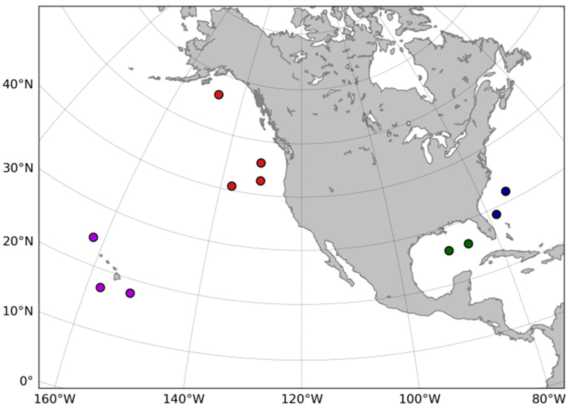
Figure 1. Position of the 11 NDBC metocean buoys selected. Different colors help to separate different clusters with different wave climates. The same color patterns will be used throughout this paper to identify the buoys’ locations.
Remotesensing 15 02203 g001
Figure 2. Autocorrelation as a function of time lags for U10 (A) and Hs (B). The 11 buoys are presented, and the gray shading shows the average of all the buoy results.
Remotesensing 15 02203 g002
Figure 3. Normalized root mean square difference as a function of the time lags for U10 (A) and Hs (B). The 11 buoys are presented, and the gray shading shows the average of all the buoy results.
Remotesensing 15 02203 g003
Figure 4. Variance spectra of U10 (A) and Hs (B) for each buoy.
Remotesensing 15 02203 g004
Figure 5. Examples of interesting events measured by the wave buoys. Four clusters and four different events are illustrated, related to hourly time-series of Hs (meters). (A) Hurricane Sandy measured in the Atlantic Ocean. (B) Hurricane Ida in the Gulf of Mexico. (C) Extra-tropical cyclone in the Pacific Ocean. (D) High-energy swell in the Tropical Pacific Ocean (Hawaii).
Remotesensing 15 02203 g005
Figure 6. Scatter plot of time-displaced time-series compared to the original time-series for different time lags ranging from 1 h to 24 h. Data of U10 (m/s) for buoy 41010. The plots use hot colors to highlight areas of higher point density. Panels (AF) show the increasing time lag.
Remotesensing 15 02203 g006
Figure 7. Scatter plot of time-displaced time-series compared to the original time-series for different time lags ranging from 1 h to 24 h. Data of Hs (m) for buoy 41010. The plots use hot colors to highlight areas of higher point density. Panels (AF) show the increasing time lag.
Remotesensing 15 02203 g007
Figure 8. Expected differences as a function of distance (km) for U10 (m/s) and Hs (m). The left panels (A,D) present scatter plots with altimeter measurements (JASON3) compared to the closest altimeter record to the buoys’ positions for each altimeter track section. The plots use hot colors to highlight areas of higher point density. The center panels (B,E) show the median (black) of such differences (altimeter–altimeter) accompanied by the shaded area designed between the first and third quartiles, while the dashed red line represents the median difference between altimeter and buoy. The use of the median for this type of analysis was suggested by Quartly and Kurekin [72]. The right panels (C,F) display the arithmetic mean of differences (altimeter–altimeter), highlighted for the first 50 km.
Remotesensing 15 02203 g008
Figure 9. Number of altimeter points in the satellite transects defined by different spatial criteria.
Remotesensing 15 02203 g009
Figure 10. Scatter plots of altimeter data for different spatial criteria (radius, km) using JASON3 dataset collocated at the 11 buoy positions (Figure 1). The plots were made using the smallest radius of 10 km as a reference. A total of 189 collocated values were used. (AD) (top) refer to wind speed (U10) while (EH) (bottom) refer to significant wave height (Hs).
Remotesensing 15 02203 g010
Figure 11. Scatter index (Equation (4)) versus bias (or mean difference, Equation (2)) for spatial criteria ranging from 10 to 200 km. The estimates calculated with the spatial criterion of 10 km were used as a reference ( x in Equations (2)–(5)). Satellite dataset considered is from JASON3. (A) Wind speed (U10). (B) Significant wave height (Hs).
Remotesensing 15 02203 g011
Figure 12. QQ-plots (A,C) and scatter plots (B,D) of collocated altimeter data of Hsc from the AODN-calibrated dataset, against NDBC buoy data in the Pacific and Atlantic Oceans (Figure 1). The temporal collocation criterion r = 1800 s was applied, and two spatial collocation criteria of τ = 25 and 50 km are presented. The plots use hot colors to highlight areas of higher point density.
Remotesensing 15 02203 g012
Table 1. Information on each NDBC buoy selected for the analyses. The distance to the nearest coast (Dcoast) and watch circle radius (WCR) are included.
BuoyIDLatitudeLongitudeDepthNDBC (m)DepthETOPO (m)Dcoast (Km)WCR (Km)Start DateN Records
4101028.90281.548909011821.2011/1988242,828
4100231.76285.16397539933533.6611/1975247,865
4200125.90270.33319432113352.8801/1976301,003
4200326.01274.35326532793153.0507/1977299,134
4600156.30212.08405440932903.9412/1974300,617
4600242.61229.51341334424863.3009/1975255,324
4600545.96229.00285227425092.7409/1976253,326
4600640.78222.604378437010884.0604/1977212,907
5100124.42197.90489549121524.6302/1981242,062
5100217.04202.30494850232954.6609/1984238,635
5100417.60207.61499850773304.9311/1984248,525
Table 2. Root mean square difference (RMSD), scatter index (SI), and correlation coefficient (CC) as a function of buoy time lag, ranging from 1 to 12 h. The bold center value represents the average result for the 11 buoys, while the two numbers in parentheses indicate the minimum and maximum values observed among the 11 buoys.
tlag (h)RMSD (m)SI 1CC
Hs10.18 (0.11,0.25)0.077 (0.065,0.083)0.982 (0.964,0.989)
20.22 (0.14,0.32)0.097 (0.071,0.113)0.974 (0.958,0.979)
30.27 (0.18,0.41)0.118 (0.078,0.144)0.963 (0.950,0.970)
60.40 (0.24,0.62)0.175 (0.099,0.225)0.920 (0.903,0.934)
120.59 (0.33,0.93)0.261 (0.136,0.343)0.825 (0.784,0.858)
tlag (h)RMSD (m/s)SI 1CC
U1011.02 (0.82,1.10)0.138 (0.102,0.163)0.938 (0.908,0.955)
21.29 (0.96,1.44)0.175 (0.120,0.207)0.902 (0.876,0.922)
31.51 (1.07,1.79)0.204 (0.132,0.243)0.868 (0.851,0.889)
62.02 (1.30,2.57)0.271 (0.161,0.320)0.769 (0.737,0.836)
122.63 (1.54,3.49)0.353 (0.190,0.423)0.613 (0.516,0.771)
1 Since bias is close to zero, the scatter index (SI) and the normalized RMSD converge to the same value.
Table 3. Results of statistical metrics (from Equations (2)–(5)) for four spatial collocation criteria compared to the 10 km reference criterion. The analysis used satellite data from JASON3.
Dist (km)BiasRMSDSICC
Hs25−0.0080.0900.0890.991
50−0.0140.1150.1140.986
100−0.0220.1490.1470.976
200−0.0600.2010.1910.960
U10250.0040.1330.0240.998
500.0080.2750.0500.993
1000.0520.4470.0810.981
2000.0950.6340.1140.963
Table 4. Validation of collocated altimeter values against buoy data using the temporal collocation criterion r = 1800 s and two spatial collocation criteria of τ = 25 and 50 km. The single altimeter records closest to the buoy positions (nearest) are included as a means of comparison, and the three averaging methods are shown. The results for four metrics (Equations (2)–(5)) are provided for Hs and the calibrated Hs (Hsc). The hot colors highlight the worst results while the best ones are presented in green.
Dist (km)MethodBiasRMSESICC
Hs25Nearest0.0360.2590.1100.977
Mean0.0380.2260.0960.983
LIDW0.0380.2280.0960.982
GF0.0380.2280.0970.982
50Nearest0.0240.2730.1120.974
Mean0.0240.2360.0960.981
LIDW0.0240.2360.0960.981
GF0.0240.2350.0960.981
Hsc25Nearest0.0130.2470.1060.979
Mean0.0150.2100.0900.985
LIDW0.0150.2120.0910.984
GF0.0150.2130.0920.984
50Nearest0.0130.2590.1060.977
Mean0.0140.2180.0890.983
LIDW0.0140.2180.0890.983
GF0.0140.2180.0890.984
Table 5. Validation of collocated altimeter values against buoy data using the temporal collocation criterion r = 1800 s and two spatial collocation criteria of τ = 25 and 50 km. The single altimeter records closest to the buoy positions (nearest) are included as a means of comparison, and the three averaging methods are shown. The results for four metrics (Equations (2)–(5)) are provided for U10 and the calibrated U10 (U10c). The hot colors highlight the worst results while the best ones are presented in green.
Dist (km)MethodBiasRMSESICC
U1025Nearest−0.3561.9560.2700.809
Mean−0.3561.9360.2680.811
LIDW−0.3561.9400.2680.811
GF−0.3561.9410.2680.811
50Nearest−0.4902.0400.2770.792
Mean−0.4892.0160.2740.794
LIDW−0.4902.0170.2740.795
GF−0.4902.0180.2750.795
U10c25Nearest0.7391.7010.1860.893
Mean0.7391.6690.1820.896
LIDW0.7391.6760.1830.895
GF0.7391.6770.1830.895
50Nearest0.7601.7210.1840.888
Mean0.7611.6810.1790.892
LIDW0.7601.6840.1790.892
GF0.7601.6850.1800.892
Table 6. Total number of collocated matchups of JASON3 altimeter data at 11 buoys presented in Figure 1 for four temporal criteria (in minutes) and four spatial criteria (in kilometers).
Time/Dist102550100
152945671134
30930183636727344
6022264389878117,553
120 12,71425,32350,583
Disclaimer/Publisher’s Note: The statements, opinions and data contained in all publications are solely those of the individual author(s) and contributor(s) and not of MDPI and/or the editor(s). MDPI and/or the editor(s) disclaim responsibility for any injury to people or property resulting from any ideas, methods, instructions or products referred to in the content.