Article

Can Plot-Level Photographs Accurately Estimate Tundra Vegetation Cover in Northern Alaska?

by
Hana L. Sellers
1,*,
Sergio A. Vargas Zesati
2,
Sarah C. Elmendorf
3,
Alexandra Locher
1,
Steven F. Oberbauer
4,
Craig E. Tweedie
2,
Chandi Witharana
5 and
Robert D. Hollister
1
1
Department of Biological Sciences, Grand Valley State University, 1 Campus Dr., Allendale, MI 49401, USA
2
Department of Biological Sciences and the Environmental Science and Engineering Program, The University of Texas at El Paso, 500 W University Ave., El Paso, TX 79968, USA
3
Institute of Arctic and Alpine Research, University of Colorado, Boulder, CO 80309, USA
4
Department of Biological Sciences and Institute of Environment, Florida International University, 11200 SW 8th St., Miami, FL 33199, USA
5
Department of Natural Resources and the Environment, University of Connecticut, Storrs, CT 06269, USA
*
Author to whom correspondence should be addressed.
Remote Sens. 2023, 15(8), 1972; https://doi.org/10.3390/rs15081972
Submission received: 22 February 2023 / Revised: 31 March 2023 / Accepted: 6 April 2023 / Published: 8 April 2023
(This article belongs to the Special Issue Advanced Technologies in Wetland and Vegetation Ecological Monitoring)

Abstract

:
Plot-level photography is an attractive time-saving alternative to field measurements for vegetation monitoring. However, widespread adoption of this technique relies on efficient workflows for post-processing images and the accuracy of the resulting products. Here, we estimated relative vegetation cover using both traditional field sampling methods (point frame) and semi-automated classification of photographs (plot-level photography) across thirty 1 m2 plots near Utqiaġvik, Alaska, from 2012 to 2021. Geographic object-based image analysis (GEOBIA) was applied to generate objects based on the three spectral bands (red, green, and blue) of the images. Five machine learning algorithms were then applied to classify the objects into vegetation groups, and random forest performed best (60.5% overall accuracy). Objects were reliably classified into the following classes: bryophytes, forbs, graminoids, litter, shadows, and standing dead. Deciduous shrubs and lichens were not reliably classified. Multinomial regression models were used to gauge if the cover estimates from plot-level photography could accurately predict the cover estimates from the point frame across space or time. Plot-level photography yielded useful estimates of vegetation cover for graminoids. However, the predictive performance varied both by vegetation class and whether it was being used to predict cover in new locations or change over time in previously sampled plots. These results suggest that plot-level photography may maximize the efficient use of time, funding, and available technology to monitor vegetation cover in the Arctic, but the accuracy of current semi-automated image analysis is not sufficient to detect small changes in cover.

1. Introduction

The Arctic is changing in response to warmer temperatures caused by global warming [1]. Warmer temperatures in the Arctic have resulted in longer growing seasons, greater permafrost degradation and active layer thaw depth, and altered snow cover and accumulation, which have the potential to influence the composition of tundra vegetation communities [2,3,4,5]. As the composition shifts in tundra vegetation communities, climate-related feedback cycles may be amplified, prompting widespread change in and beyond the Arctic [6,7]. To assess and forecast change across a warming Arctic, monitoring plant cover, structure, and community dynamics over time is critical [1,8].
Time series of satellite-derived spectral indices, which are proxies for vegetation cover and biomass, have shown greening in the Arctic tundra for more than 40 years [9,10], while spectral browning has been detected in boreal regions [11,12,13]. Spectral greening trends suggest an increase in vegetation productivity as a result of warming, whereas spectral browning trends suggest a decrease in vegetation productivity [14]. Satellite-based observations and trends must be validated by ground-based observations, but these data do not always correspond spatially or temporally [14].
How patterns detected by satellites are related to patterns observed on the ground is not well understood due to the mismatch among spatial resolution, spatial coverage, and remote sensing approaches. A dearth of sustained surface or near-surface observations of vegetation change has limited further exploration of this scaling mismatch and uncertainty [15,16,17,18]. Analyses of repeat plot-level photographs and both occupied and unoccupied aircraft have been identified for their potential to bridge the data gap between ground-based and satellite-based observations in the Arctic [19,20,21,22,23].
Ground-based observations can be used as a reference standard to validate remotely sensed observations due to the precise, accurate, and repeatable nature of such measurements [24,25]. The point frame method is a standard field technique for measuring in situ vegetation cover in the Arctic [26]. Although this method is accurate, repeatable, and robust, it is time-consuming and requires a high level of training and experience to implement effectively [27]. Generating a sufficiently large, representative sample size using this method is a challenge since vegetation plots are likely to be sampled at a lower spatial and temporal frequency [27]. Additionally, traditional approaches to vegetation monitoring in the Arctic are constrained by a multitude of factors that include, but are not limited to, a short growing season (less than three months), extensive logistical costs, and limited access to remote research sites. These challenges have increasingly catalyzed the adoption of remote sensing methods in the Arctic [28,29,30].
Plot-level photography requires less time and less extensive training than traditional vegetation sampling methods and has the capacity to increase the spatiotemporal extent and resolution of vegetation surveys. Repeat photography can be analyzed retroactively and is less prone to observer bias than sustained field surveys [31,32,33,34]. Plot-level photographs are also advantageous because nadir image acquisition can capture complete vegetation cover within a given field of view, whereas the analysis of point frame data is limited to the point density of the sampling frame [31,35].
Image analysis has transitioned from pixel-based to object-based over recent years [36,37]. Object-based image analysis, developed in the biomedical and computer sciences, has been adapted for the analysis of remotely sensed imagery, with geographic object-based image analysis (GEOBIA) as the accepted framework [36,37,38]. Image objects are generated from groups of homogeneous pixels through segmentation and then assigned to a class through classification. Spatial, spectral, and other features within an image, additional data layers, and expert user knowledge can be incorporated into the classification procedure, which further offsets object-based from pixel-based approaches [39].
As high spatial resolution imagery becomes more accessible due to technological advancements, the application of GEOBIA has become more common due to its advantages over other approaches [40,41,42]. Although GEOBIA has been applied extensively to classify vegetation cover in aerial and satellite imagery [43], relatively few studies have applied GEOBIA to near-surface plot-level imagery [32,35,44], especially in polar regions [23,31,34].
Chen et al. (2010) [31] applied object-based image analysis to plot-level photographs acquired in the Arctic in 2007. The cover estimates of a few dominant vegetation species from plot-level photographs were compared using a digital grid overlay, ocular estimates of plant cover in the field, and an object-based image segmentation scheme in which objects were automatically derived from photographs and then manually classified to species by a botanist. The object-based approach was the most accurate in estimating differences in species-specific leaf area index (LAI) over space, but it was also the most time-consuming of the three methods due to the large manual component. They did not evaluate the accuracy of the methods by assessing the changes in vegetation cover over time.
More recently, King et al. (2020) [34] applied object-based image analysis to plot-level photographs acquired in Antarctica from 2003 to 2014. The authors created a rule-based framework where user-defined thresholds were applied to classify objects into healthy, stressed, and moribund bryophyte covers. The remaining four classes (lichens, rock, shadow, and snow) were manually digitized and masked from the images. This framework is not applicable to most tundra communities because tundra vegetation tends to exhibit greater species diversity, especially among vascular plants, than Antarctica [45,46]. Manual digitization of tundra vegetation in plot-level photographs is unlikely to be a feasible solution, as classes are more numerous, complex, and do not possess visually distinctive boundaries. An accuracy assessment using in situ field survey data was not included in King et al. (2020) [34].
Here, we extend previous work by applying semi-automated image analysis to the vegetation in northern Alaska, quantifying the cover of eight complex vegetation classes from plot-level photographs across nearly a decade. We evaluate the accuracy of plot-level photography using in situ field survey data from the point frame method. Finally, we use the estimates of vegetation cover from the plot-level photographs to predict vegetation cover over space and time, scaling our approach to tundra communities with similar composition.
We address the following questions:
  • Which machine learning model is optimal for the classification of plot-level photographs of Arctic tundra vegetation?
  • How do estimates from plot-level photography compare with estimates from the point frame method?
  • Can we predict vegetation cover across space and time using the vegetation cover estimates from plot-level photography?

2. Materials and Methods
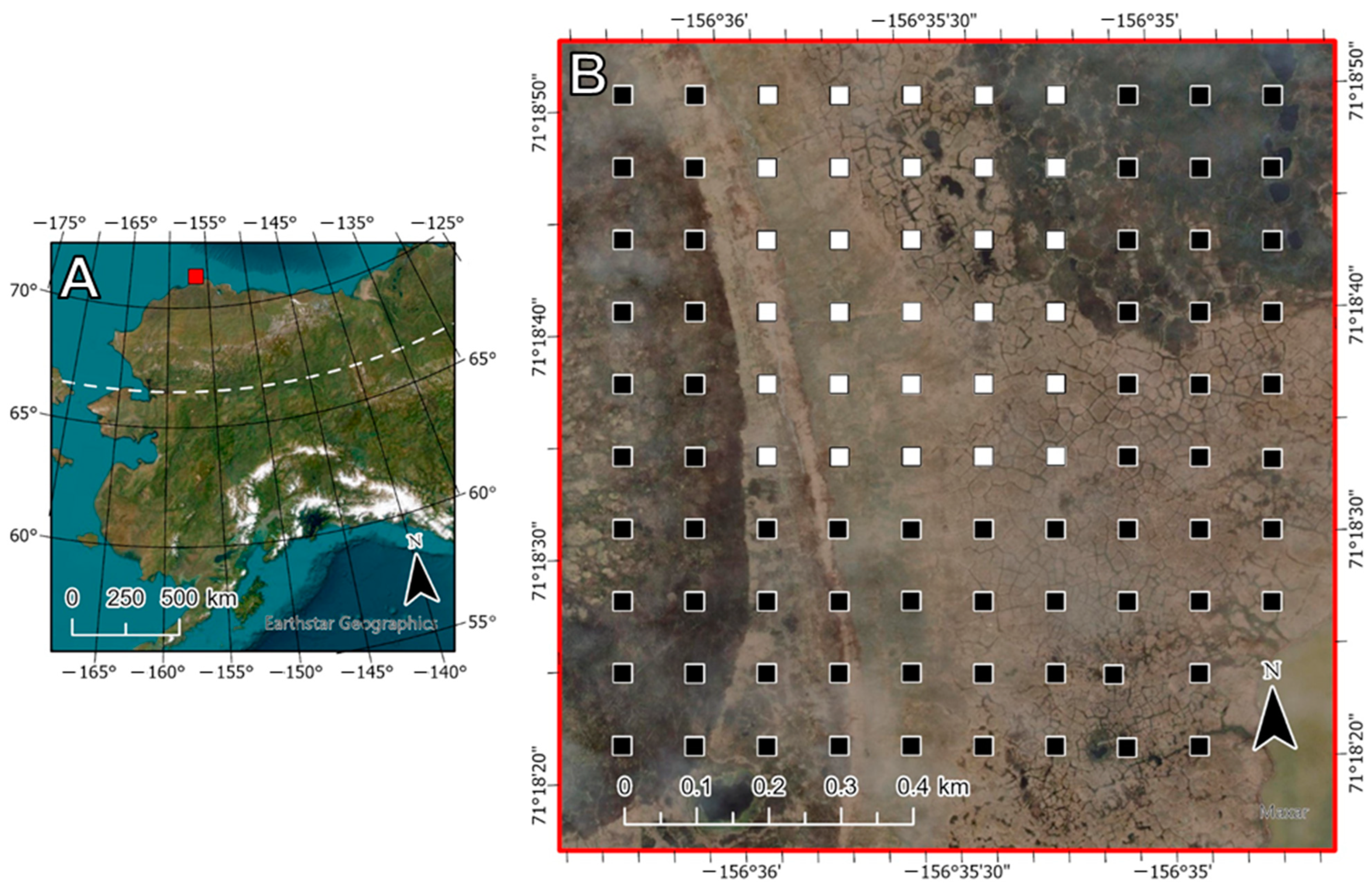
2.1. Study Site

In the early 1990s, a sampling grid was established at Utqiaġvik (formerly Barrow), Alaska (71°19′N, 156°36′W) by the Arctic System Science (ARCSS) program to monitor long-term, landscape-level terrestrial change [47]. Ninety-eight 1 m2 vegetation plots were installed at 100-meter intervals across the 1 km2 sampling grid in 2010 (Figure 1). The 98 plots are sampled once every five years due to the tremendous effort and expense of vegetation sampling using the point frame method [27,48]. Of the original 98 plots, a subset of 30 plots was selected for annual vegetation sampling, which evenly represented four generalized vegetation communities based on a classification map developed from a 2002 QuickBird satellite image [49]. The 30 plots are the focus of this study. Furthermore, we examine vegetation cover and change within a 0.75 m2 footprint in each 1 m2 plot, as the point frame only spans 0.75 m2.
This region is classified as a wetland dominated by sedges, grasses, and mosses (class W1) by the Circumpolar Arctic Vegetation Map [50]. Average July temperatures for the region were historically recorded at 4 °C, although the region has experienced a warming trend over the past several decades [1,51,52]. Continuous daylight is exhibited in the Arctic for most of the growing season, which extends from early June to late August. Peak growing season, when the plants are generally greenest and most productive, occurs from July through mid-August [53].

2.2. Plot-Level Photography

Plot-level photographs were taken at waist height (approximately 1 m above the ground), from a near nadir perspective, centered above the plot. Although overcast conditions were preferred to reduce the amount of shadow in the photograph, lighting conditions were not always consistent. An object-based approach may combat inconsistent lighting by relying on information that is independent of color, which reduces the error associated with inconsistent lighting conditions [34].
Plot-level photographs were taken using either a Panasonic DMC-TS3 or Nikon Coolpix AW120 handheld camera. Images were considered high resolution since the objects of interest were at least three to five times larger than the number of pixels in the objects [40,54,55]. Automatic camera settings (no flash, fixed focus) were used to respond to natural ambient light in the environment. Images were recorded as uncompressed JPEG files with three visible spectral bands (red, green, and blue) and an 8-bit, unsigned radiometric resolution, which ranged in digital values from 0 to 255.
Plot-level photographs were mostly collected on a biweekly basis during the growing season (Table S1). One set of plot-level photographs near the peak growing season was analyzed each year, although some substitutions occurred for photographs that were not vertically positioned, missing, or out-of-focus (Figure S1). Photographs were substituted if an adjacent sampling date contained an acceptable image. In total, 210 plot-level photographs were analyzed across seven sampling years (2012, 2013, 2014, 2015, 2018, 2019, and 2021). In 2016, no photographs were recorded. In 2017, photographs were not suitable because they were taken prior to peak greenness and productivity. In 2020, photographs were of low resolution and incomplete.

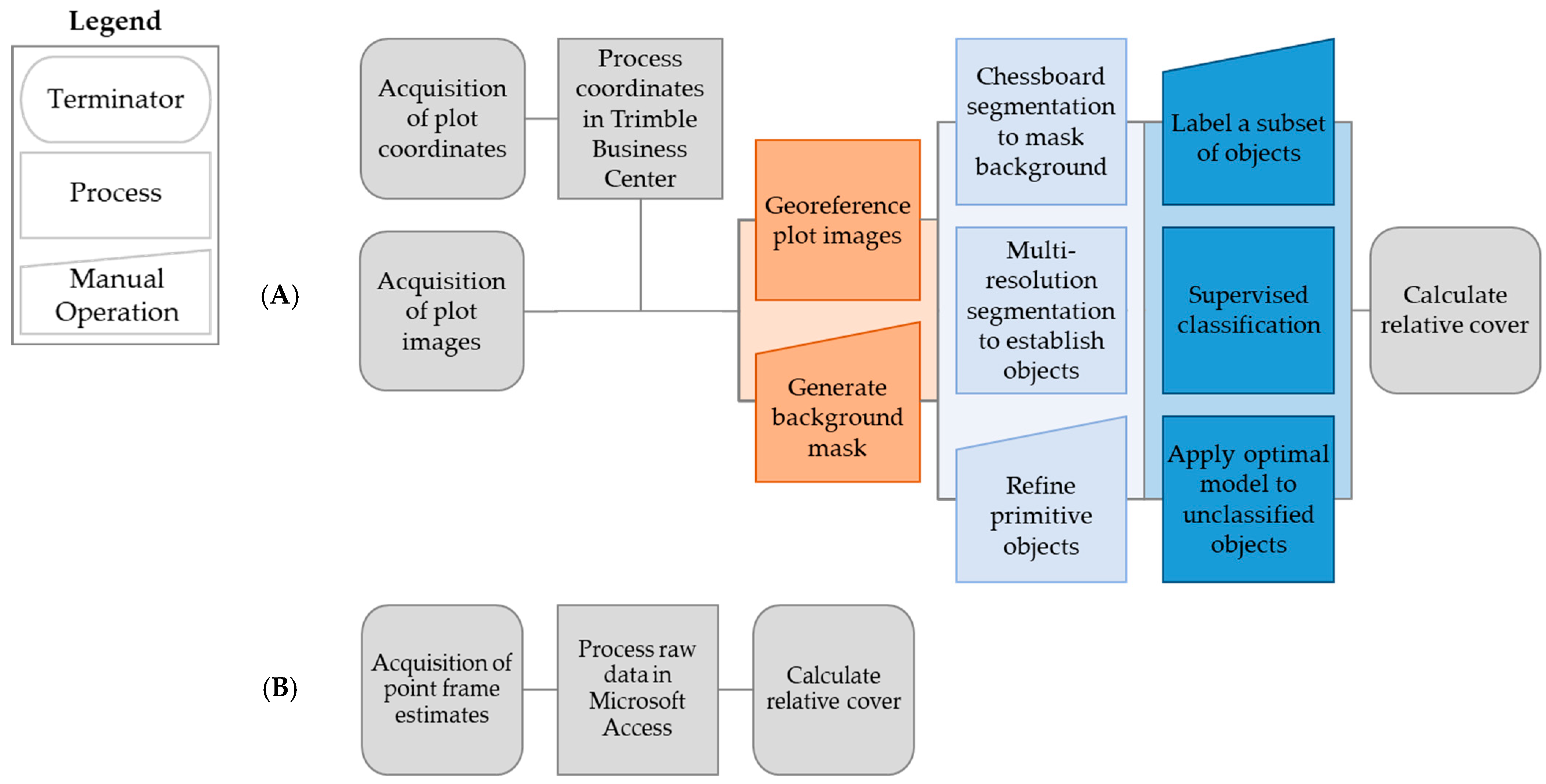
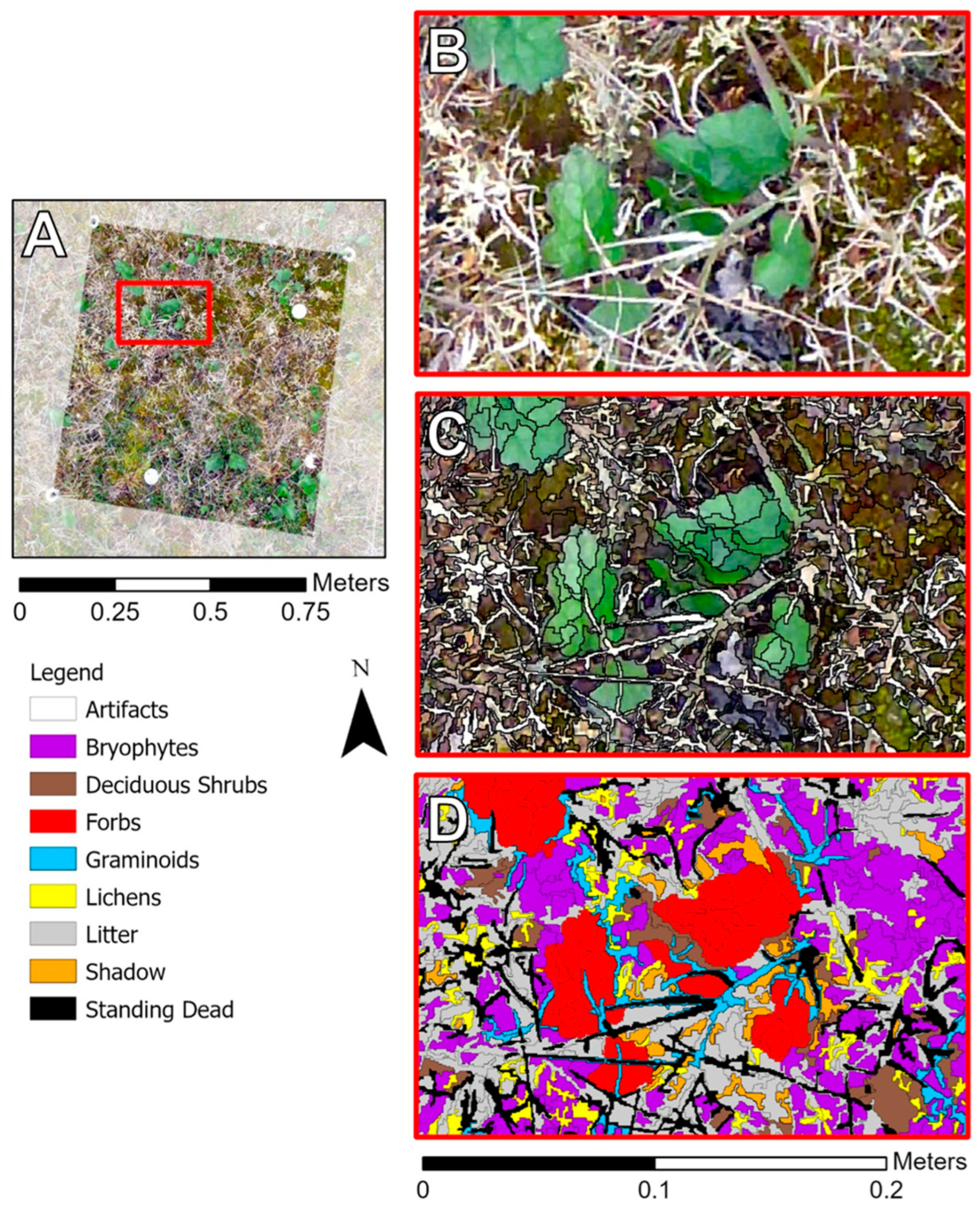
2.3. Semi-Automated Image Analysis

2.3.1. Image Preprocessing

Images were geometrically corrected in ArcGIS Pro v. 2.8 (ESRI Inc.; Redlands, CA, USA). Each image was registered to four ground control points, or differential global positioning system (DGPS) coordinates, which marked the plot corners. The base of each stake was surveyed using high-precision coordinates collected with a Trimble R8 GNSS receiver and a 2 m survey pole in 2013. Despite some tilt over time due to freeze-thaw cycles, the base of the stakes remained permanently fixed. Coordinates were processed using the Post Processing Kinematic (PPK) approach in Trimble Business Center v. 2.70, with an overall accuracy of 1 to 5 cm (Trimble; München, Germany).
Permanent physical tags in each vegetation plot delineate a 0.75 m2 footprint and help realign the position of the point frame during annual field sampling (Figure S2). The tags established additional ground control points within the plot images to improve alignment of the images across all other years. Nearest neighbor resampling rectified the pixel sizes of all images to a coarser resolution of 0.05 cm, which standardized the resolution and allowed for direct comparison between images [34,35]. Images and their corresponding background mask templates were exported for use in eCognition (Figure 2).
Orthorectification is preferred for accurate registration because it establishes a true nadir perspective and reduces the likelihood of an over- or under-valuation of plant cover [56]. Although orthorectification is critical for a reliable analysis of pixel-to-pixel change, it is not critical for a reliable analysis of change in relative vegetation cover [34,57]. We assessed the total number of objects, not the change between pixels, so the georeferencing procedure is acceptable for our analysis [34].

2.3.2. Segmentation and Preliminary Classification

An object-based approach was applied to the plot-level photographs in eCognition Developer v. 9.5 (Trimble; München, Germany) (Figure 3). Using the background mask templates exported from ArcGIS Pro, chessboard segmentation was applied to mask the exterior of each vegetation plot in eCognition. Then, image objects were generated from the interior of the vegetation plot using the multi-resolution segmentation algorithm, which is one of the most widespread and successful segmentation algorithms for GEOBIA [58,59]. Image objects undergo an iterative algorithm in which pixels are grouped into objects until the threshold (defined by scale) is reached. The threshold (scale) is user-defined and weighted by shape and compactness.
Scale is unit-less, not intuitive, and depends on the heterogeneity of the image. In general, a lower value for scale results in smaller objects, whereas a higher value for scale results in larger objects. Shape values range from 0 to 1. A higher value for shape generates objects that are weighted more heavily by shape, whereas a lower value for shape generates objects that are weighted more by color. Compactness ranges from 0 to 1. Lower compactness values generate objects that are squiggly and irregular. Higher compactness values generate objects that are blocky, rectangular, and compact.
Although supervised and unsupervised approaches have been proposed for the automatic, objective selection of optimal segmentation parameters, there is no consensus within the remote sensing community [60]. We applied a supervised, stepwise approach to select the optimal segmentation parameters for our images. Although some researchers argue that this method may lack repeatability and robustness, a trial-and-error approach to maximize parameters can provide strong results [40,61,62].
All variables were held constant while independently adjusting each of the user-defined parameters to observe the effect of each parameter on the image objects. The final parameters, used consistently across all the images, were scale: 30, color/shape: 0.5/0.5, smoothness/compactness: 0.7/0.3. Color and shape were equally adept at creating logical image objects. A greater weight was assigned to smoothness since tundra vegetation is rarely blocky or square.
After segmentation, we established a non-hierarchical, multi-class classification scheme that contained ten classes: bryophytes, deciduous shrubs, forbs, graminoids, lichens, litter, non-vegetation, shadow, standing dead, and water. Vascular plants (deciduous shrubs, forbs, and graminoids) and non-vascular species (bryophytes and lichens) were grouped by broad growth form. Litter and standing dead resulted from dead plant material, but these two classes can be classified separately since they differ in characteristics and structure. Standing dead is typically recognizable by its reflective upright stalks, while litter may be so degraded that it is unrecognizable.
Inflorescences may appear identical or vastly different in shape, color, and size as a result of their development within their phenological lifespan. Due to the low frequency and lack of pattern among the inflorescences, all inflorescences were identified manually and classified into the corresponding vegetation class. Images also contained a variety of non-vegetation classes at low frequencies (insects, animal excrement, bare ground, fungi, and permanent tags), but these classes were not common enough to properly train a machine learning model. Instead, non-vegetation and water were manually identified and masked from each image. In the rare event that an object was unidentifiable from the image, it was also classified as non-vegetation. Finally, areas obscured by shadow were not able to be accurately identified, so shadow was assigned its own class. In the rare event that a mixed image object was encountered in the labeling procedure, the image object was classified based on the majority class [63].

2.3.3. Machine Learning Classification

The caret package assembles a wide variety of classification and regression models into a standard framework using universal syntax for R [64]. Auxiliary tasks such as data preparation, data splitting, variable selection, and model evaluation are also integrated into this package. We relied on caret to train, validate, and test the classification models. Five machine learning models were implemented in this study: random forest (RF), gradient boosted modeling (GBM), classification and regression tree (CART), support vector machine (SVM), and k-nearest neighbor (KNN) (Table S2). A sampling grid was applied to most models to find the best hyperparameters, which were tuned using the validation data subset.
A total of 15,000 image objects were selected randomly and equally across all the plot images, which was approximately 0.7% of the total data set (N = 2,159,693 image objects). The image objects were visually identified by an expert as belonging to one of the eight classes and then divided into training (70%), validation (15%), and test (15%) subsets using a random sampling scheme stratified by class. As a general rule for large data sets, a minimum of 10,000 samples must be sampled [65]. There were also at least 50 samples per class, but most classes exceeded 75 to 100 samples, which is optimal for larger data sets [65]. To adjust for class imbalance, classes were downsampled to the number of image objects in the least prevalent class for model training and validation.
A combination of spectral, shape, and textural features, which leverage the information in an object-based approach, were selected for analysis (Table S3). Texture features were calculated from a gray-level co-occurrence matrix (GLCM) [66,67]. A GLCM tabulates how often different combinations of pixel gray levels appear or exist in an image or scene. Contrast features include homogeneity, contrast, and dissimilarity, while orderliness features include entropy and the angular second moment. Texture features were calculated from all bands in all directions (0°, 45°, 90°, and 135°) and therefore show directional invariance.
Several band combinations, or spectral indices, were tested using the visible red, green, and blue bands. Spectral indices may minimize the effects of uneven illumination [68]. Some spectral indices can provide an estimation of vegetation cover, phenological shifts, or productivity, while others can help distinguish soil or non-living elements from living vegetation species [19,69,70,71,72,73,74].
Features may be highly correlated in eCognition, so redundancies must be closely examined and eliminated during model development [75,76]. Features above a 95% correlation threshold were removed from analysis, resulting in 22 features for further exploration. Since the data set in this study was not high-dimensional, it was not critical to remove features through more rigorous testing [43,77].
We evaluated the model performance of five machine learning models using five repeats of 10-fold cross validation. We compared the performance metrics (i.e., overall accuracy and Kappa) of the machine learning models using paired t-tests, which were adjusted for multiple comparisons via the Bonferroni correction.
Machine learning models were scored based on their overall accuracy (OA) and Kappa. Overall accuracy indicates the number of image objects that were classified correctly. An accuracy greater than 80% is a strong model, a value between 80% and 40% is moderate, and a value less than 40% is poor [63]. Kappa accounts for the possibility of agreement between the reference and classified data sets based on chance.
The highest-performing model in terms of overall accuracy was applied to the total data set to classify each image. We summarized the individual class accuracy from the top-performing model in terms of producer accuracy and user accuracy, which are the complements of the omission and commission error rates, respectively [78]. Producer accuracy (PA) describes the probability that a real-life object is classified correctly in the image, whereas user accuracy (UA) describes the probability that a classified object in an image matches the object in real-life.

2.4. Point Frame

Vegetation cover in the field was assessed using the point frame method [26,27,48]. A gridded frame of 0.75 m2 was aligned to permanent physical tags in each vegetation plot. The frame was leveled and positioned above the tallest plant species in the plot. A hundred nodes, or sampling points, were distributed equally every 7.5 cm on the gridded frame. A wooden rod was dropped at every node. Species identity, height, and live or dead status were recorded for each encounter until the ground was reached. Plots were sampled once within the same 14-day time frame annually from mid-July through early August.
Relative vegetation cover estimates were processed in Microsoft Access 2019 (Microsoft Corp.; Redmond, WA, USA). Plant species were grouped into seven broad growth forms, or vegetation classes: bryophytes, deciduous shrubs, forbs, graminoids, lichens, litter, and standing dead. Encounters with research equipment, permanent physical tags, and open water were removed from the data set prior to calculations of relative cover. Relative cover refers to the total cover of each vegetation class divided by the total cover of all vegetation classes in a plot.

2.5. Predicting Vegetation Cover

Vegetation cover in the field was assessed using the point frame method, yielding count-based measurements of cover. Count-based cover data are often zero-inflated and do not conform to standard distributions. Negative covariances among taxonomic groups are expected since the relative covers must sum to one. Therefore, a growing number of studies have advocated for the use of the Dirichlet–multinomial model for analysis of over-dispersed, count-based cover data [79,80].
We applied direct substitution and multinomial logistic regression to predict vegetation cover. Direct substitution assumes a 1:1 correspondence between relative cover values from the point frame and plot-level photography. However, we also anticipated that the measurements from plot-level photography might not be directly interchangeable with the measurements from the point frame due to the height and often complex structure of the plant canopy. Therefore, we calibrated the relationship between the two methods using vegetation cover estimates from both the point frame and plot-level photography in the multinomial model.
Here, we used multinomial logistic regression to model (y) the point frame estimates of cover for all vegetation classes using the image-based estimates of the cover for all vegetation classes from the corresponding plots at each sampling time as predictors (x). The resulting fitted model was then used to generate predictions of relative cover in each vegetation plot in each year (plot-year). Although the multinomial models were fitted directly to the point frame counts, we used relative rather than absolute cover to evaluate model performance, as the null expectation is that the total number of counts in any given vegetation class will be higher when more points are sampled in a plot.
We evaluated model performance using out-of-sample methods. We evaluated predictive performance over space or time to understand how plot-level photography might be used to extend spatial or temporal monitoring. We partitioned the data set temporally using an end-sample holdout method [81], using the first three years to fit the model and the last four years for evaluation. We used a similar fraction to partition the data set spatially, using a random 3/7 of the plots for fitting (13 plots) and the remaining 4/7 for evaluation (17 plots). We calculated the mean absolute error (MAE) and bias of estimates of the relative cover of each vegetation plot in each year in the holdout set using either direct substitution or the predictions from the multinomial model, which were calibrated on the training dataset.
To recommend plot-level photography as a substitute for the point frame method, it is required that its performance meet the precision criterion for each application. We therefore used mean absolute error (MAE) and bias as criteria to evaluate the utility of estimating relative cover using plot-level photography [82]. MAE was calculated as the average absolute difference between the predicted relative cover of vegetation in each class and the observed relative cover in each class (mean(|(predicted − observed)|)). Bias was calculated as the mean difference between the two relative covers in each class ((mean(predicted − observed))). Bias describes whether a predicted class was over- or under-estimated by the model since bias accounts for directionality.
As a final test to gauge what information can be gained through plot-level photography, we asked whether using plot-level photographs to estimate vegetation cover in unsampled plots or years, using either direct substitution or multinomial logistic regression, improved estimates of vegetation cover vis-à-vis a null model where we assumed that the cover in the unsampled plots or years of the validation dataset was equal to the training-set mean. The training-set mean is an estimate derived without plot-level photography data, so it provides a direct way to estimate how much vegetation cover estimates are improved with the addition of plot-level photographs. For the temporal comparison, we estimated the relative cover of each vegetation class in each test plot-year as the mean over 2012–2014 of the point frame relative cover per vegetation class for the corresponding plot. For the spatial comparison, we estimated the relative cover of each vegetation class in each test plot-year as the annual mean of the point frame relative cover per vegetation class of all the training plots for the corresponding year.
Multinomial logistic models were fitted using the nnet package in R v. 7.3-14 (R Core Team; Vienna, Austria). While other packages (e.g., various Bayesian methods) can incorporate random effects into multinomial models, we did not get satisfactory model convergence using plot and year random effects. The computational time was substantially higher than the nnet implementation, too. Incorporation of random effects was not essential because our design was balanced and models were compared using MAE and bias, not the statistical significance of regression parameters.

3. Results

3.1. Comparing Machine Learning Models

The random forest model performed the best, with an overall accuracy of 60.5% (Table 1). The gradient boosted model performed slightly worse, with an overall accuracy of 59.8%. The computational time was greatest for the gradient boosted model. The k-nearest neighbor model was the worst-performing model with an overall accuracy of 46.6%. All models were statistically different based on multiple comparisons of their overall accuracies, or Kappa values (p ≤ 0.05), except for the random forest and gradient boosted models.
In general, most classes demonstrated individual class accuracy above 50% using the optimal random forest model (Table 2). Graminoids and litter exhibited high user accuracy, and bryophytes exhibited moderate user accuracy. Deciduous shrubs had the lowest producer accuracy (40.0%) and user accuracy (15.6%). Deciduous shrubs were most frequently confused with bryophytes (22.9% of the time), graminoids (33.5% of the time), and litter (21.6% of the time) in the classification. There was less confusion between deciduous shrubs and forbs than anticipated (3.2% of the time). Lichens also had an unusually low user accuracy (20.4%); this class was most frequently confused with litter (39.8% of the time) and standing dead (23.1% of the time) in the classification.
Shadow was rarely confused with the other classes. Shadow was most frequently confused with bryophytes (17.7% of the time) and litter (11.3% of the time). Shadows varied with light intensity and canopy structure and were present to some degree in all images. Shadow occupied between 0.36% and 41.8% of a plot image (mean = 11.5%). The least amount of shadow overall (7.3% total) occurred in the images from 2013, while images from 2018 had the most shadow (16.7% total).
Intensity was ranked as the feature with the highest relative importance (Table 3). The top five most important features were spectral or layer values. Texture features were ranked in the middle, while most of the geometric predictors were ranked at the bottom.

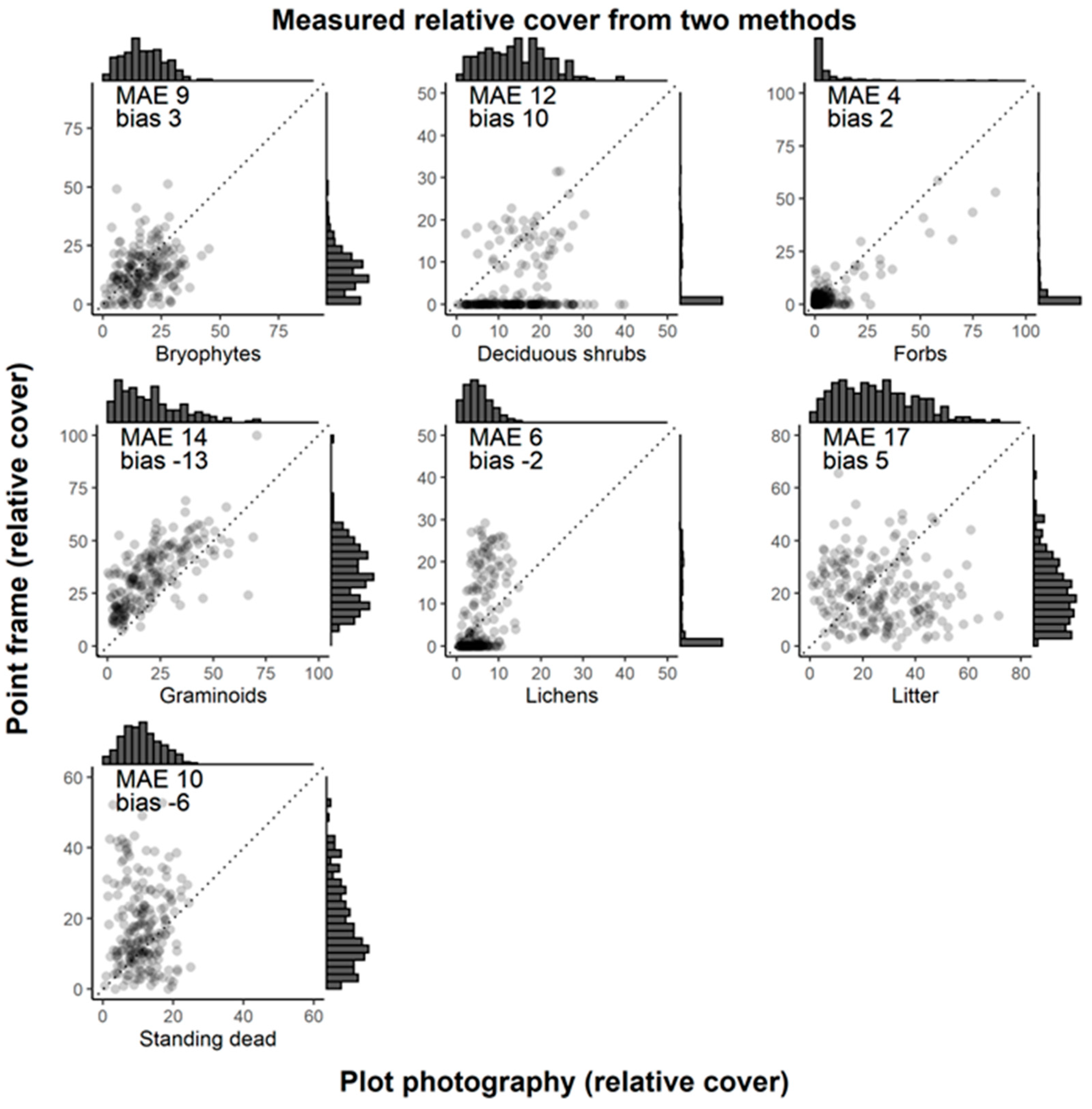
3.2. Comparing Estimates of Vegetation Cover from Plot-Level Photography and Point Frame Sampling

Combining data over space (plots) and time (years), there were clear differences between vegetation classes in the degree of correspondence between cover as estimated from plot-level photographs versus point frame sampling in the field (Figure 4). For example, there was little correspondence between litter estimates using the two methods, whereas the same plot-years tended to have high amounts of graminoids using both methods. Plot-level photography generally tended to underestimate the relative cover of graminoids.
Testing the out-of-sample performance of plot-level photography to estimate vegetation cover indicated that using multinomial regression to predict point frame vegetation cover generally led to better estimates than direct substitution and, in many cases, provided a more precise estimate of point frame cover than a null model. However, the utility of the plot-level photographs varied by vegetation class and whether unsampled locations or years were tested. Out-of-sample performance of the regression models over time demonstrated that image-based estimates lowered the MAE without increasing the bias for all classes except for bryophytes and standing dead vis-à-vis raw substitution (Figure S3). The modeled image-based estimates provided lower MAE values than the temporal variability for graminoids, litter, and standing dead (Table 4). Out-of-sample performance of the regression models over space demonstrated that image-based estimates lowered the MAE without increasing the bias for all classes except for forbs vis-à-vis raw substitution (Figure S4). The modeled image-based estimates provided lower MAE values than the spatial variability for graminoids, shrubs, and lichens (Table 4).

4. Discussion

We estimated the cover of eight major plant growth forms on 1 m2 plots using semi-automated image analysis of plot-level photographs and the traditional point frame method. This study is one of few examining fine-scale tundra vegetation cover using remote sensing techniques. Tundra vegetation has complex characteristics and structure that can make objects difficult to identify using supervised object-based classification [28,83]. The semi-automated image analysis pipeline consisted of machine learning models that were evaluated against a data set of segmented objects derived from plot-level photographs that were manually identified. The results are discussed in terms of overall model performance (Section 4.1) and the individual class accuracies of each vegetation class (Section 4.2). We also compare the vegetation cover estimates from plot-level photography against the estimates from the point frame method (Section 4.3) and then predict vegetation cover over space and time using multinomial models (Section 4.4). Finally, we discuss the sources of error (Section 4.5) and provide recommendations for future studies (Section 4.6).

4.1. Comparing Machine Learning Models

We analyzed several machine learning classification models and found that random forest was optimal for plot-level photographs of tundra vegetation. Although the random forest and gradient boosted models were not statistically different from one another, the random forest had the highest overall accuracy and a reasonable run time (Table 1). Our results are consistent with other published work, where random forest had the best performance in comparison to other common models.
A systematic comparison by Li et al. (2016) [84] revealed that ensemble-based models, such as random forest (bagging) or Adaboost (boosting), exhibited the highest classification accuracy. Support vector machines also exhibited high classification accuracy [84]. Although simple decision trees can prove accurate across different segmentation scales [85], they are often unstable at fine scales, yielding even poorer results if mixed objects are present in the data set [84]. K-nearest neighbor, which was a popular machine learning model in early studies due to its computational simplicity and ease of use within the eCognition framework [86], generally appears unsuitable for classification due to low average accuracies in comparison to other models [43]. These results corroborate the performance trend across the models in our study.
On average, our reported classification accuracy was lower than other published studies using supervised object-based classification. However, most existing studies are focused on a larger scale and have more clearly observed differences between classes [42]. Many factors influence the performance and overall accuracy of a model, including the scale of segmentation, feature selection, and the homogeneity of objects [84,87]. Classification accuracy can also depend on image quality and the characteristics and complexity of the land cover types in the images [43]. Our classification accuracy may have suffered as the vegetation classes in our study are complex. There were mixed objects in our images as a result of segmentation, which lowers classification accuracy [84]. Homogeneous objects or landscapes, such as the repetitive patterns in agricultural fields, often have higher classification accuracy. Classification accuracy also tends to decrease as the total number of classes increases, especially above four [88]. Our study contained ten classes before two (non-vegetation and water) were manually eliminated from the scheme.
As expected, spectral features were the most influential predictors in the random forest classification. Spectral features measure the fundamental properties of the objects, while texture measures the spatial relationships of pixels within an object. These features are more likely to be independent and complement each other [85,89]. Shape features had the least impact on the random forest classification, which validates the theory that shape features may become more critical at greater scales [87]. Importance values should be interpreted with care, since highly correlated, continuous predictors may be given higher values erroneously [90]. eCognition produces features that can be highly correlated; therefore, our analysis discusses feature importance in broad terms only [76,91].
Hue, saturation, and intensity (value), or HSV, have been shown to improve the segmentation or classification of digital images [31,35,75]. HSV results from a transformation of the red, green, and blue color spaces, which are highly correlated bands and tend to provide redundant information [92]. HSV did not improve the segmentation of the plot-level photographs in our preliminary analysis. However, hue and intensity were both among the top five predictors of the classification. Intensity showed significant, distinctive contrast between vegetation classes at a cursory glance, especially in comparison to other spectral, textural, or geometric features. In general, shadows and standing dead were on opposite ends of the spectrum for intensity values.
Green ratio, green-red vegetation index (GRVI), and greenness excess index (GEI) were also among the top five predictors. These indices measure similar information, regarding the phenology and vegetation composition, from the plot-level photographs. GRVI has performed comparably to the normalized difference vegetation index (NDVI) at the plot-level; thus, GRVI can be used interchangeably with NDVI, usually at the expense of lower overall accuracy [19,93,94]. The green ratio, GRVI, and GEI offer important, discriminatory information on the vegetation classes based on their high importance values. Perhaps, these RGB-based indices may be used as proxies to NIR-based indices when standard, low-cost cameras are used to capture photographic information from vegetation plots.

4.2. Reliability of Vegetation Classes

Using the optimal random forest model, we found that six classes were reliably identified from the semi-automated image analysis of plot-level photography: bryophytes, forbs, graminoids, litter, shadows, and standing dead (Table 2). Graminoids are the most abundant vegetation class at Utqiaġvik. If graminoids can be classified accurately using this technique, then the impact of this dominant vegetation class can be better quantified across the landscape. However, we were unable to reliably identify the vegetation classes: deciduous shrubs and lichens (Table 2). Deciduous shrubs were often confused with other objects that exhibited a similar size and shape. Deciduous shrubs were often over-segmented, and perhaps a clear delineation of deciduous shrubs may improve this classification error. Perhaps more instances of lichens were needed to train the model, given the variety of different species at Utqiaġvik, which vary by color and structure [95]. Image analysis and machine and deep learning approaches are expected to improve over time and may allow for accurate classification of these two problematic vegetation classes, provided that the images are available for analysis.
The results of the classification may have improved if the focus had been on living vegetation only. Standing dead and litter can be difficult to identify using automatic pattern recognition. Standing dead is primarily composed of graminoids and old inflorescences, which tend to be tall, narrow, and reflective. Litter encompasses all dead plant material that has fallen to the bottom of the canopy. Litter may appear round, brown, and curled shortly after senescence or gray and formless as plant material degrades over time. Not only is it difficult to establish a repeatable classification pattern for the machine learning models, but the boundaries of this class may also be difficult to define during segmentation.
Shadows have been shown to confuse image analysis and lower classification accuracy [35]. Shadows are a common component of plot-level photography. Even in ideal, overcast sampling conditions, shadows remained visible in the middle and lower canopies in the digital images. It is difficult to achieve standardized lighting conditions in the Arctic, where fieldwork is limited by a short growing season, inconsistent cloud cover, and low sun angles [96]. Blocking direct sunlight to standardize lighting conditions may be possible with additional equipment or a second field technician, but shadows cannot be eliminated from the images, only minimized [31,32,34,35]. In this study, shadow was its own class, and very little class confusion occurred except for some overlap with bryophyte and litter cover. Bryophytes vary in color and texture, especially in response to moisture level [97]. Inundated bryophytes tend to darken in color, creating a more complicated task for the machine learning model to distinguish an inundated bryophyte from a shadow. Litter appeared not to have a distinctive color, shape, or size since it can vary depending on the degree of degradation and the vegetation composition. Litter tends to be darker in color due to degradation, so the class confusion with shadow was also justified. It may be possible to improve the distinction between shadow, bryophytes, and litter with additional training samples.

4.3. Comparing Estimates of Vegetation Cover from Plot-Level Photography and Point Frame Sampling

The comparison cannot be made directly between the cover estimates from the point frame and plot-level photography methods of sampling. Each biomass encounter, or contact, was recorded throughout the entire depth of the plant canopy using the point frame sampling method [27,48]. Then, vegetation cover was assumed for each cell on the sampling grid based on the number of contact hits within each cell. Plot-level photographs only recorded the topmost visible layer but were not constrained to a sampling grid of 100 cells. Because the spatial resolution differed between the point frame and plot-level photography, the relative cover from the point frame may not be identical to the relative cover that was obtained through image analysis [31]. The timing of vegetation sampling using the point frame and plot-level photography methods was often offset, which could introduce further differences.
The change in relative cover must be interpreted carefully for both sampling methods [31,44]. Canopy density and species diversity may influence the cover estimates. A plant can grow at different heights, angles, and locations within plots, which may influence its detectability over space and time. Therefore, rarer vegetation classes, such as deciduous shrubs, may be detected using the point frame method during some years but not all. Additionally, short-statured growth forms, such as bryophytes and lichens, can be hidden beneath the topmost visible layer, rendering them invisible to the camera. The differences in sampling techniques between the point frame and plot-level photography methods may explain the weaker associations between the relative cover estimates of some of the vegetation classes.

4.4. Using Plot-Level Photography to Predict Vegetation Cover across Space and Time

To recommend plot-level photography as a substitute for more labor-intensive point frame sampling in the field, plot-level photography must yield accurate and unbiased estimates of vegetation cover. Because acceptable levels of error and bias are likely to vary based on application, we opted to compare estimates of vegetation cover derived from plot-level photographs to a baseline estimate that assumes composition is static over either space or time, following best practices for ecological forecasting [98]. We found image analysis can be used to reliably estimate the cover of graminoids. Plot-level photography can also characterize the large variability of deciduous shrub and lichen cover across the landscape and the large variability of litter and standing dead cover over time. We tested our approach on a subset of thirty vegetation plots in the ARCSS grid. This subset is sampled once annually using the point frame method and up to six times seasonally using the plot-level photography method. In contrast, the ninety-eight vegetation plots in the ARCSS grid are sampled once every five years using the point frame method, since this requires a large investment in terms of field crew, time, energy, and logistics. The performance of the holdout space model on the thirty vegetation plots strongly suggests that plot-level photographs could be used to estimate deciduous shrub, forb, and lichen cover on the remaining sixty-five vegetation plots.
For most vegetation classes, individual plots had a relatively static composition over time. As a result, plot-level photographs did not provide improved estimates of annual vegetation cover. Exceptions were graminoids, litter, and standing dead, where plot-level photography estimates tracked temporal shifts. While unbiased estimates of relative cover were generated using plot-level photography, the estimates were not precise on a per-plot level and lacked sufficient accuracy to capture more subtle shifts in vascular vegetation over time within individual plots for all groups except graminoids. Improvements to our image analysis approach may also improve the accuracy of the image-based estimates, thereby improving how well the estimates predict relative cover on a per-plot level. Thus, plot-level photography is a useful but imperfect method of sampling tundra landscapes. It may add more information spatially, where there is a large compositional turnover, than temporally, where the cover changes are subtler.

4.5. Additional Sources of Error

In addition to the sources of error discussed above, some uncertainties accumulate throughout semi-automated image analysis. Manual object labeling was executed by an expert with substantial field experience and skill in Arctic plant identification. Therefore, interpretation errors were inevitable but consistent across the data set. The root mean square error (RMSE) averaged 1.5 to 4.8 cm across sampling years due to the georeferencing procedure (Table S4). In a few cases, the RMSE extended to 8.8 to 11.5 cm on the images with the most severe distortion as a result of poor camera angles. Positional errors also resulted from the error inherent in the DGPS coordinates (1 to 5 cm). Positional errors can be minimized but not eliminated.
Accurate segmentation provides a better chance of accurate classification. In this study, the user-dependent segmentation parameters affected the shape and size of objects, therefore affecting the quality and number of objects generated. Perhaps a more rigorous set of rules can be included to refine the primitive image objects in the early steps of the object-based approach. The segmentation parameters can also be optimized using a formal segmentation accuracy assessment [87,99]. Our approach to image analysis was limited by both the available data set and tools of analysis, and we expect that it will be modified and improved over time.
Errors were also inevitable using the point frame sampling method. Positional errors were minimized due to precise leveling and alignment of the point frame with permanent tags in the vegetation plot. Point frame sampling can also be intensive and tiring, so interpretation errors were possible due to the exhaustion of the field technician [100,101]. Tall vegetation can shift with the wind, so the frequency of contact hits may be skewed during windy conditions [102]. A misclassification can result when the field technician records incorrect information about the vegetation composition of the plot. Even so, these errors are generally minimal and are usually rectified in post-processing pipelines. There is strong evidence that vegetation composition and cover at the plot-level are monitored accurately using this method of sampling [103].

4.6. Recommendations for Future Image Analysis

Recent studies have suggested that the accuracy of segmentation is assessed through a formal accuracy assessment [87,99]. Not only can this assessment vary according to the user, but it is often time-consuming for complex images since a formal accuracy assessment may require the manual delineation of an independent set of reference polygons. Although the accuracy of segmentation is an important consideration in image analysis, not all researchers agree that a formal accuracy assessment is necessary [40,62]. Nevertheless, an accuracy assessment would be a useful consideration for future studies.
Artificial neural networks could be explored in future comparative studies, perhaps leading to a classification with increased accuracy. Neural networks require large, uncorrelated data sets and an in-depth understanding of the mechanism underpinning the classifier to obtain concrete, reliable results [91,104,105]. Neural networks can be easily over- or undertrained, resulting in spurious, noisy, and non-reproducible results [104,105]. We aim to optimize the accuracy of our segmentation before we further investigate neural networks, as neural networks can be highly sensitive to the quality of the training data set [106]. This remains to be studied in future works.
We encountered some limitations within ArcGIS Pro and eCognition, so our approach to image analysis was not fully contained within either platform. We could not create a random selection of objects in eCognition, nor could we extend this to a scale that encompassed all the images in this study. We also found that the processing time to export the feature list for each image was long and computationally intensive in eCognition. The classification models also lacked the requisite transparency to understand and validate the statistics. The limitations of eCognition were remedied by R, thus the image analysis pipeline transitions between the three platforms (Figure 2). Moving forward, our aim is to increase the repeatability, robustness, and accuracy of the image analysis in this study. We seek to automate the procedure by transferring our approach from local image processing (ArcGIS Pro, eCognition, and R) to cloud-based image processing using high-performance computing, where Python is the preferred language.
Automatic identification and removal of water from the plot images is preferred to manual digitization and removal. The near-infrared (NIR) band would improve the efficiency of our semi-automatic image processing routine. The Normalized Difference Water Index (NDWI), a water-specific index, has been used to identify and remove standing water from remotely sensed images [107,108]. The NIR band would also permit us to calculate and explore the impact of the Normalized Difference Vegetation Index (NDVI), which is a widely used metric to monitor vegetation dynamics across the Arctic [109,110]. The band combinations that we can use are limited to the visible electromagnetic spectrum and contain a finite amount of information. While we can maintain the analysis of historic photographs with visible red, green, and blue bands, we can also benefit from technological improvements in our equipment (i.e., multispectral sensors or LiDAR), which might allow us to access more information across the electromagnetic spectrum, thereby improving our classification and providing valuable insights into tundra plant canopy and characteristics.
Unoccupied aerial vehicles (UAV), or drones, may be an effective alternative to plot-level photography. Drones are likely to be adopted as a tool to sample vegetation in the Arctic, as there is an increasing need for daily, flexible data collection and integration of geospatial information across observation platforms [14,20,21,29]. The potential benefits of drones include rapid acquisition of high-resolution images, greater ground coverage, and a lower impact on existing vegetation, soil, and permafrost, as drones can be operated from a single launch location. With a few necessary modifications, we expect that drone imagery can be processed using the semi-automated image analysis pipeline from this study. In the future, we seek to examine if drone imagery can validate tundra vegetation cover and change, as detected using point frame and plot-level photography, to scale our results from the ground to an aerial level.

5. Conclusions

An object-based approach was applied to high-resolution plot-level photographs with three spectral bands (red, green, and blue) to estimate the relative cover of eight vegetation classes. The random forest model performed better than the other machine learning models (gradient boosted model, classification and regression tree, support vector machine, and k-nearest neighbor) with an overall accuracy of 60.5%. Although the random forest model required more processing time than most of the other models, the overall accuracy was significantly higher in comparison. The gradient boosted model performed similarly, but at the expense of a greater computational load and processing time, which made this model less desirable for future use. In this study, random forest is the optimal machine learning model for plot-level photographs of tundra vegetation.
Although the overall accuracy of our classifications was lower than the supervised object-based classifications of various land cover types in previous studies [43], the separation of plant growth forms is much more difficult due to mixed objects in a complex matrix at a fine scale. Vegetation classes (bryophytes, deciduous shrubs, forbs, graminoids, lichens, litter, and standing dead) were also composed of many individual species, which have different forms and characteristics. Most comparable published studies have the added benefit of hyperspectral or multispectral bands, which results in more information to use in the classification [111,112]. Since our spectral information was limited to red, green, and blue bands only, we expected lower classification accuracy.
Some vegetation classes were reliably classified using plot-level photography and semi-automated image analysis, but not all. Bryophytes, forbs, graminoids, litter, shadow, and standing dead were reliably classified, while deciduous shrubs and lichens were not. Perhaps a larger training data set or improvements to the shape or size of objects might improve the individual class accuracy of problematic vegetation classes, thereby improving the overall accuracy of the classification. We recommend including a comprehensive accuracy assessment for segmentation parameters in future studies [87,99].
RGB-based spectral indices and layer values were the most influential in the classification. Geometric and textural features were less influential in the random forest classification; that is, these features complemented existing spectral information to a limited degree. Therefore, we submit that valuable information can be gained through standard imagery, which only consists of red, green, and blue spectral bands. However, technological improvements to our digital cameras could improve our semi-automatic image analysis routine and classification results in the future if we could access more of the electromagnetic spectrum, notably the NIR band.
Standardized image collection methods may also improve our results. In the point frame sampling method, positional errors were minimized by precise leveling and alignment with permanent tags in the vegetation plots. Although exact duplication of a scene is not necessary to measure vegetation cover and change, minimizing the positional differences of the digital camera may reduce the positional error of the plot-level photographs, ultimately improving our analysis of vegetation change. Perhaps a tripod with levels attached to the frame and camera would offer more control and consistency.
Plot-level photography is a useful but imperfect method of sampling. Comparisons to point frame estimates of vegetation cover revealed that the object-based approach to analyzing the plot-level photographs is useful for some applications, but it requires improvement before being used interchangeably with field sampling. Plot-level photography may add more information spatially, where there is a large compositional turnover, than temporally, where the cover changes are subtler. These limitations are likely not restricted to plot-level photography. Assessments of remote sensing techniques to detect temporal changes in plant biodiversity, rather than spatial comparisons, are rare due to the short duration of most field sampling campaigns [113]. However, strong temporal variability in the ability to detect grassland biodiversity based on hyperspectral remote sensing has also been reported [114]. Our results also suggest that monitoring biodiversity change over time using remote sensing techniques may be more difficult than documenting spatial patterns. Given the urgency of understanding biodiversity loss and the rapid development of new remote sensing platforms specifically targeting biodiversity monitoring [115,116], we emphasize the importance of multi-year comparisons of field-based and remote sensing-based biodiversity change studies to fully understand the potential and limitations for change detection.
A photographic record can be revisited and reanalyzed in the future, and it is versatile, quick, and cost-effective. An object-based approach to image analysis provides reliable, although limited, information from high-resolution plot-level photographs of tundra vegetation. Information from plot-level photographs can complement existing field observations. Integrating both techniques is expected to maximize time, funding, and technology to monitor terrestrial change in the Arctic.

Supplementary Materials

Supplementary figures and tables are available for download at: https://www.mdpi.com/article/10.3390/rs15081972/s1. Figure S1: Examples of unacceptable plot-level photographs; Figure S2: Image of a plot; Figure S3: Model performance predicting the point frame cover in holdout years; Figure S4: Model performance predicting the point frame cover in holdout plots; Table S1: Vegetation sampling dates; Table S2: List of machine learning models applied; Table S3: List and explanation of the features calculated for each image object; Table S4: Amount of positional error in each plot-level photograph.

Author Contributions

Conceptualization, H.L.S., S.A.V.Z., S.C.E., A.L. and R.D.H.; Formal Analysis, H.L.S. and S.C.E.; Resources, C.W.; Writing—original draft, H.L.S., S.C.E. and R.D.H.; Writing—review and editing, all authors; Funding acquisition, S.F.O., C.E.T. and R.D.H. All authors have read and agreed to the published version of the manuscript.

Funding

This research was funded by the Office of Polar Programs of the National Science Foundation (grant numbers: 0856516, 0856628, 1432277, 1433330, 1504224, 1504345, 1836839, and 1836861).

Data Availability Statement

The point frame data from this study are available in the Arctic Data Center at https://doi.org/10.18739/A2MG7FX0Q.

Acknowledgments

Field logistics were provided by UIC Science. We thank the current and former field technicians of the Arctic Ecology Program (Grand Valley State University) and the Systems Ecology Lab (University of Texas at El Paso) for assistance with data collection. We also thank Ryan Cody and Mariana Mora (University of Texas at El Paso) and Katlyn Betway-May (Grand Valley State University) for providing clean data sets. We thank Kin M. Ma (Grand Valley State University) for his technical assistance with computer software.

Conflicts of Interest

The authors declare no conflict of interest.

References

  1. Constable, A.J.; Harper, S.; Dawson, J.; Holsman, K.; Mustonen, T.; Piepenburg, D.; Rost, B. Cross-Chapter Paper 6: Polar Regions. In Climate Change 2022: Impacts, Adaptation and Vulnerability; Pörtner, H.O., Roberts, D.C., Tignor, M., Poloczanska, E.S., Mintenbeck, K., Alegría, A., Craig, M., Langsdorf, S., Löschke, S., Möller, V., et al., Eds.; Cambridge University Press: New York, NY, USA, 2022; pp. 2319–2368. [Google Scholar]
  2. Kelsey, K.; Pedersen, S.; Leffler, A.J.; Sexton, J.; Feng, M.; Welker, J.M. Winter Snow and Spring Temperature Have Differential Effects on Vegetation Phenology and Productivity across Arctic Plant Communities. Glob. Chang. Biol. 2021, 27, 1572–1586. [Google Scholar] [CrossRef] [PubMed]
  3. Leffler, A.J.; Klein, E.S.; Oberbauer, S.F.; Welker, J.M. Coupled Long-Term Summer Warming and Deeper Snow Alters Species Composition and Stimulates Gross Primary Productivity in Tussock Tundra. Oecologia 2016, 181, 287–297. [Google Scholar] [CrossRef] [PubMed]
  4. Shiklomanov, N.I.; Streletskiy, D.A.; Nelson, F.E.; Hollister, R.D.; Romanovsky, V.E.; Tweedie, C.E.; Bockheim, J.G.; Brown, J. Decadal Variations of Active-Layer Thickness in Moisture-Controlled Landscapes, Barrow, Alaska. J. Geophys. Res. 2010, 115, G00I04. [Google Scholar] [CrossRef]
  5. Farquharson, L.M.; Romanovsky, V.E.; Cable, W.L.; Walker, D.A.; Kokelj, S.V.; Nicolsky, D. Climate Change Drives Widespread and Rapid Thermokarst Development in Very Cold Permafrost in the Canadian High Arctic. Geophys. Res. Lett. 2019, 46, 6681–6689. [Google Scholar] [CrossRef] [Green Version]
  6. Chapin, F.S.; Sturm, M.; Serreze, M.C.; McFadden, J.P.; Key, J.R.; Lloyd, A.H.; McGuire, A.D.; Rupp, T.S.; Lynch, A.H.; Schimel, J.P.; et al. Role of Land-Surface Changes in Arctic Summer Warming. Science 2005, 310, 657–660. [Google Scholar] [CrossRef]
  7. Pearson, R.G.; Phillips, S.J.; Loranty, M.M.; Beck, P.S.A.; Damoulas, T.; Knight, S.J.; Goetz, S.J. Shifts in Arctic Vegetation and Associated Feedbacks under Climate Change. Nat. Clim. Chang. 2013, 3, 673–677. [Google Scholar] [CrossRef]
  8. Post, E.; Alley, R.B.; Christensen, T.R.; Macias-Fauria, M.; Forbes, B.C.; Gooseff, M.N.; Iler, A.; Kerby, J.T.; Laidre, K.L.; Mann, M.E.; et al. The Polar Regions in a 2 °C Warmer World. Sci. Adv. 2019, 5, aaw9883. [Google Scholar] [CrossRef] [Green Version]
  9. Guay, K.C.; Beck, P.S.A.; Berner, L.T.; Goetz, S.J.; Baccini, A.; Buermann, W. Vegetation Productivity Patterns at High Northern Latitudes: A Multi-Sensor Satellite Data Assessment. Glob. Chang. Biol. 2014, 20, 3147–3158. [Google Scholar] [CrossRef] [Green Version]
  10. Zhu, Z.; Piao, S.; Myneni, R.B.; Huang, M.; Zeng, Z.; Canadell, J.G.; Ciais, P.; Sitch, S.; Friedlingstein, P.; Arneth, A.; et al. Greening of the Earth and Its Drivers. Nat. Clim. Chang. 2016, 6, 791–795. [Google Scholar] [CrossRef]
  11. Bhatt, U.S.; Walker, D.A.; Raynolds, M.K.; Bieniek, P.A.; Epstein, H.E.; Comiso, J.C.; Pinzon, J.E.; Tucker, C.J.; Polyakov, I.V. Recent Declines in Warming and Vegetation Greening Trends over Pan-Arctic Tundra. Remote Sens. 2013, 5, 4229–4254. [Google Scholar] [CrossRef] [Green Version]
  12. De Jong, R.; de Bruin, S.; de Wit, A.; Schaepman, M.E.; Dent, D.L. Analysis of Monotonic Greening and Browning Trends from Global NDVI Time-Series. Remote Sens. Environ. 2011, 115, 692–702. [Google Scholar] [CrossRef] [Green Version]
  13. Phoenix, G.K.; Bjerke, J.W. Arctic Browning: Extreme Events and Trends Reversing Arctic Greening. Glob. Chang. Biol. 2016, 22, 2960–2962. [Google Scholar] [CrossRef] [Green Version]
  14. Myers-Smith, I.H.; Kerby, J.T.; Phoenix, G.K.; Bjerke, J.W.; Epstein, H.E.; Assmann, J.J.; John, C.; Andreu-Hayles, L.; Angers-Blondin, S.; Beck, P.S.A.; et al. Complexity Revealed in the Greening of the Arctic. Nat. Clim. Chang. 2020, 10, 106–117. [Google Scholar] [CrossRef] [Green Version]
  15. Epstein, H.E.; Raynolds, M.K.; Walker, D.A.; Bhatt, U.S.; Tucker, C.J.; Pinzon, J.E. Dynamics of Aboveground Phytomass of the Circumpolar Arctic Tundra during the Past Three Decades. Environ. Res. Lett. 2012, 7, 015506. [Google Scholar] [CrossRef]
  16. Fisher, J.B.; Hayes, D.J.; Schwalm, C.R.; Huntzinger, D.N.; Stofferahn, E.; Schaefer, K.; Luo, Y.; Wullschleger, S.D.; Goetz, S.; Miller, C.E.; et al. Missing Pieces to Modeling the Arctic-Boreal Puzzle. Environ. Res. Lett. 2018, 13, 020202. [Google Scholar] [CrossRef] [Green Version]
  17. Walker, D.A.; Daniëls, F.J.A.; Alsos, I.; Bhatt, U.S.; Breen, A.L.; Buchhorn, M.; Bültmann, H.; Druckenmiller, L.A.; Edwards, M.E.; Ehrich, D.; et al. Circumpolar Arctic Vegetation: A Hierarchic Review and Roadmap toward an Internationally Consistent Approach to Survey, Archive and Classify Tundra Plot Data. Environ. Res. Lett. 2016, 11, 055005. [Google Scholar] [CrossRef]
  18. Wu, X.; Xiao, Q.; Wen, J.; You, D.; Hueni, A. Advances in Quantitative Remote Sensing Product Validation: Overview and Current Status. Earth Sci. Rev. 2019, 196, 102875. [Google Scholar] [CrossRef]
  19. Anderson, H.B.; Nilsen, L.; Tommervik, H.; Rune Karlsen, S.; Nagai, S.; Cooper, E.J. Using Ordinary Digital Cameras in Place of Near-Infrared Sensors to Derive Vegetation Indices for Phenology Studies of High Arctic Vegetation. Remote Sens. 2016, 8, 847. [Google Scholar] [CrossRef] [Green Version]
  20. Assmann, J.J.; Myers-Smith, I.H.; Kerby, J.T.; Cunliffe, A.M.; Daskalova, G.N. Drone Data Reveal Heterogeneity in Tundra Greenness and Phenology Not Captured by Satellites. Environ. Res. Lett. 2020, 15, 125002. [Google Scholar] [CrossRef]
  21. Cunliffe, A.M.; Assmann, J.J.; Daskalova, G.N.; Kerby, J.T.; Myers-Smith, I.H. Aboveground Biomass Corresponds Strongly with Drone-Derived Canopy Height but Weakly with Greenness (NDVI) in a Shrub Tundra Landscape. Environ. Res. Lett. 2020, 15, 125004. [Google Scholar] [CrossRef]
  22. Fraser, R.H.; Olthof, I.; Lantz, T.C.; Schmitt, C. UAV Photogrammetry for Mapping Vegetation in the Low-Arctic. Arct. Sci. 2016, 2, 79–102. [Google Scholar] [CrossRef] [Green Version]
  23. Liu, N.; Treitz, P. Modeling High Arctic Percent Vegetation Cover Using Field Digital Images and High Resolution Satellite Data. Int. J. Appl. Earth Obs. 2016, 52, 445–456. [Google Scholar] [CrossRef]
  24. Malenovský, Z.; Lucieer, A.; King, D.H.; Turnbull, J.D.; Robinson, S.A. Unmanned Aircraft System Advances Health Mapping of Fragile Polar Vegetation. Methods Ecol. Evol. 2017, 8, 1842–1857. [Google Scholar] [CrossRef] [Green Version]
  25. Orndahl, K.M.; Macander, M.J.; Berner, L.T.; Goetz, S.J. Plant Functional Type Aboveground Biomass Change within Alaska and Northwest Canada Mapped Using a 35-Year Satellite Time Series from 1985 to 2020. Environ. Res. Lett. 2022, 17, 115010. [Google Scholar] [CrossRef]
  26. Molau, U.; Mølgaard, P. International Tundra Experiment (ITEX) Manual, 2nd ed.; Danish Polar Center: Copenhagen, Denmark, 1996. [Google Scholar]
  27. May, J.L.; Hollister, R.D. Validation of a Simplified Point Frame Method to Detect Change in Tundra Vegetation. Polar Biol. 2012, 35, 1815–1823. [Google Scholar] [CrossRef]
  28. Beamish, A.; Raynolds, M.K.; Epstein, H.E.; Frost, G.V.; Macander, M.J.; Bergstedt, H.; Bartsch, A.; Kruse, S.; Miles, V.; Tanis, C.M.; et al. Recent Trends and Remaining Challenges for Optical Remote Sensing of Arctic Tundra Vegetation: A Review and Outlook. Remote Sens. Environ. 2020, 246, 111872. [Google Scholar] [CrossRef]
  29. Du, J.; Watts, J.D.; Jiang, L.; Lu, H.; Cheng, X.; Duguay, C.; Farina, M.; Qiu, Y.; Kim, Y.; Kimball, J.S.; et al. Remote Sensing of Environmental Changes in Cold Regions: Methods, Achievements and Challenges. Remote Sens. 2019, 11, 1952. [Google Scholar] [CrossRef] [Green Version]
  30. Shiklomanov, A.N.; Bradley, B.A.; Dahlin, K.M.; Fox, A.M.; Gough, C.M.; Hoffman, F.M.; Middleton, E.M.; Serbin, S.P.; Smallman, L.; Smith, W.K. Enhancing Global Change Experiments through Integration of Remote-Sensing Techniques. Front. Ecol. Environ. 2019, 17, 215–224. [Google Scholar] [CrossRef] [Green Version]
  31. Chen, Z.; Chen, E.W.; Leblanc, S.G.; Henry, G.H.R.; Chen, W. Digital Photograph Analysis for Measuring Percent Plant Cover in the Arctic. Arctic 2010, 63, 315–326. [Google Scholar] [CrossRef] [Green Version]
  32. Luscier, J.D.; Thompson, W.L.; Wilson, J.M.; Gorhara, B.E.; Dragut, L.D. Using Digital Photographs and Object-Based Image Analysis to Estimate Percent Ground Cover in Vegetation Plots. Front. Ecol. Environ. 2006, 4, 408–413. [Google Scholar] [CrossRef] [Green Version]
  33. Booth, D.T.; Cox, S.E.; Fifield, C.; Phillips, M.; Willlamson, N. Image Analysis Compared with Other Methods for Measuring Ground Cover. Arid Land Res. Manag. 2005, 19, 91–100. [Google Scholar] [CrossRef]
  34. King, D.H.; Wasley, J.; Ashcroft, M.B.; Ryan-Colton, E.; Lucieer, A.; Chisholm, L.A.; Robinson, S.A. Semi-Automated Analysis of Digital Photographs for Monitoring East Antarctic Vegetation. Front. Plant Sci. 2020, 11, 766. [Google Scholar] [CrossRef]
  35. Laliberte, A.S.; Rango, A.; Herrick, J.E.; Fredrickson, E.L.; Burkett, L. An Object-Based Image Analysis Approach for Determining Fractional Cover of Senescent and Green Vegetation with Digital Plot Photography. J. Arid Environ. 2007, 69, 1–14. [Google Scholar] [CrossRef]
  36. Hay, G.J.; Castilla, G. Geographic Object-Based Image Analysis (GEOBIA): A New Name for a New Discipline. In Lecture Notes in Geoinformation and Cartography; Blaschke, T., Lang, S., Hay, G.J., Eds.; Springer: Berlin, Germany, 2008; pp. 75–89. ISBN 9783319005140. [Google Scholar]
  37. Hay, G.J.; Castilla, G. Object-Based Image Analysis: Strengths, Weaknesses, Opportunities and Threats (SWOT). In International Archives of the Photogrammetry, Remote Sensing and Spatial Information Sciences, Proceedings of the 1st International Conference on Object-Based Image Analysis (OBIA 2006), Salzburg, Austria, 4–5 July 2006; ISPRS: Hannover, Germany, 2006; pp. 1–3. [Google Scholar]
  38. Blaschke, T. Object Based Image Analysis for Remote Sensing. ISPRS J. Photogramm. Remote Sens. 2010, 65, 2–16. [Google Scholar] [CrossRef] [Green Version]
  39. Platt, R.V.; Rapoza, L. An Evaluation of an Object-Oriented Paradigm for Land Use/Land Cover Classification. Prof. Geog. 2008, 60, 87–100. [Google Scholar] [CrossRef]
  40. Blaschke, T.; Hay, G.J.; Kelly, M.; Lang, S.; Hofmann, P.; Addink, E.; Queiroz Feitosa, R.; van der Meer, F.; van der Werff, H.; van Coillie, F.; et al. Geographic Object-Based Image Analysis—Towards a New Paradigm. ISPRS J. Photogramm. Remote Sens. 2014, 87, 180–191. [Google Scholar] [CrossRef] [Green Version]
  41. Chen, G.; Weng, Q.; Hay, G.J.; He, Y. Geographic Object-Based Image Analysis (GEOBIA): Emerging Trends and Future Opportunities. GIScience Remote Sens. 2018, 55, 159–182. [Google Scholar] [CrossRef]
  42. Hussain, M.; Chen, D.; Cheng, A.; Wei, H.; Stanley, D. Change Detection from Remotely Sensed Images: From Pixel-Based to Object-Based Approaches. ISPRS J. Photogramm. Remote Sens. 2013, 80, 91–106. [Google Scholar] [CrossRef]
  43. Ma, L.; Manchun, L.; Ma, X.; Cheng, L.; Du, P.; Liu, Y. A Review of Supervised Object-Based Land-Cover Image Classification. ISPRS J. Photogramm. Remote Sens. 2017, 130, 277–293. [Google Scholar] [CrossRef]
  44. Michel, P.; Mathieu, R.; Mark, A.F. Spatial Analysis of Oblique Photo-Point Images for Quantifying Spatio-Temporal Changes in Plant Communities. Appl. Veg. Sci. 2010, 13, 173–182. [Google Scholar] [CrossRef]
  45. Alberdi, M.; Bravo, L.A.; Gutierrez, A.; Gidekel, M.; Corcuera, L.J. Ecophysiology of Antarctic Vascular Plants. Physiol. Plant. 2002, 115, 479–486. [Google Scholar] [CrossRef] [PubMed]
  46. Callaghan, T.V.; Björn, L.O.; Chernov, Y.; Chapin, T.; Christensen, T.; Huntley, B.; Ims, R.A.; Johansson, M.; Jolly, D.; Jonasson, S.; et al. Biodiversity, Distributions and Adaptations of Arctic Species in the Context of Environmental Change. Ambio 2004, 33, 404–417. [Google Scholar] [CrossRef] [PubMed]
  47. Brown, J.; Hinkel, K.M.; Nelson, F.E. The Circumpolar Active Layer Monitoring (CALM) Program: Research Designs and Initial Results. Polar Geogr. 2000, 24, 165–258. [Google Scholar] [CrossRef]
  48. Harris, J.A.; Hollister, R.D.; Botting, T.F.; Tweedie, C.E.; Betway, K.R.; May, J.L.; Barrett, R.T.S.; Leibig, J.A.; Christoffersen, H.L.; Vargas, S.A.; et al. Understanding the Climate Impacts on Decadal Vegetation Change in Northern Alaska. Arct. Sci. 2022, 8, 878–898. [Google Scholar] [CrossRef]
  49. Botting, T.F. Documenting Annual Differences in Vegetation Cover, Height and Diversity near Barrow, Alaska. Master’s Thesis, Grand Valley State University, Allendale, MI, USA, 2015. [Google Scholar]
  50. Raynolds, M.K.; Walker, D.A.; Balser, A.; Bay, C.; Campbell, M.; Cherosov, M.M.; Daniëls, F.J.A.; Eidesen, P.B.; Ermokhina, K.; Frost, G.V.; et al. A Raster Version of the Circumpolar Arctic Vegetation Map (CAVM). Remote Sens. Environ. 2019, 232, 111297. [Google Scholar] [CrossRef]
  51. Box, J.E.; Colgan, W.T.; Christensen, T.R.; Schmidt, N.M.; Lund, M.; Parmentier, F.-J.W.; Brown, R.; Bhatt, U.S.; Euskirchen, E.S.; Romanovsky, V.E.; et al. Key Indicators of Arctic Climate Change: 1971–2017. Environ. Res. Lett. 2019, 14, 045010. [Google Scholar] [CrossRef]
  52. Brown, J.; Miller, P.C.; Tieszen, L.L.; Bunnell, F.L. (Eds.) An Arctic Ecosystem: The Coastal Tundra at Barrow, Alaska; Dowden, Hutchinson & Ross, Inc.: Stroudsburg, PA, USA, 1980; pp. 1–571. [Google Scholar]
  53. Tieszan, L.L. Photosynthesis in the Principal Barrow, Alaska Species: A Summary of Field and Laboratory Responses. In Vegetation and Production Ecology of an Alaskan Arctic Tundra; Tieszen, L.L., Ed.; Springer: New York, NY, USA, 1978; pp. 241–268. [Google Scholar]
  54. Lang, S. Object-Based Image Analysis for Remote Sensing Applications: Modeling Reality—Dealing with Complexity. In Object-based Image Analysis; Blaschke, T., Lang, S., Hay, G.J., Eds.; Springer: Berlin/Heidelberg, Germany; New York, NY, USA, 2008; pp. 1–25. [Google Scholar]
  55. Strahler, A.; Woodcock, C.; Smith, J. On the Nature of Models in Remote Sensing. Remote Sens. Environ. 1986, 20, 121–139. [Google Scholar] [CrossRef]
  56. Clarke, T.A.; Fryer, J.G. The Development of Camera Calibration Methods and Models. Photogramm. Rec. 1998, 16, 51–66. [Google Scholar] [CrossRef]
  57. Rogers, G.F.; Turner, R.M.; Malde, H.E. Using Matched Photographs to Monitor Resource Change. In Renewable Resource Inventories for Monitoring Changes and Trends, Proceedings of the International Conference, Corvallis, OR, USA, 15–19 August 1983; Bell, J.F., Atterbury, T., Eds.; OSU Press: Corvallis, OR, USA, 1983; pp. 90–92. [Google Scholar]
  58. Baatz, M.; Schaape, A. A Multiresolution Segmentation: An Optimization Approach for High Quality Multi-Scale Image Segmentation. In Proceedings of the Angewandte Geographische Informations-Verarbeitung XII; Strobl, J., Ed.; University of Salzburg: Salzburg, Austria, 2000; pp. 12–23. [Google Scholar]
  59. Benz, U.C.; Hofmann, P.; Willhauck, G.; Lingenfelder, I.; Heynen, M. Multi-Resolution, Object-Oriented Fuzzy Analysis of Remote Sensing Data for GIS-Ready Information. ISPRS J. Photogramm. Remote Sens. 2004, 58, 239–258. [Google Scholar] [CrossRef]
  60. Hossain, M.D.; Chen, D. Segmentation for Object-Based Image Analysis (OBIA): A Review of Algorithms and Challenges from Remote Sensing Perspective. ISPRS J. Photogramm. Remote Sens. 2019, 150, 115–134. [Google Scholar] [CrossRef]
  61. Liu, T.; Abd-Elrahman, A.; Morton, J.; Wilhelm, V.L. Comparing Fully Convolutional Networks, Random Forest, Support Vector Machine, and Patch-Based Deep Convolutional Neural Networks for Object-Based Wetland Mapping Using Images from Small Unmanned Aircraft System. GIScience Remote Sens. 2018, 55, 243–264. [Google Scholar] [CrossRef]
  62. Radoux, J.; Bogaert, P. Good Practices for Object-Based Accuracy Assessment. Remote Sens. 2017, 9, 646. [Google Scholar] [CrossRef] [Green Version]
  63. Congalton, R.G.; Green, K. Assessing the Accuracy of Remotely Sensed Data: Principles and Practices, 3rd ed.; Lewis Publishers: Boca Raton, FL, USA, 2019. [Google Scholar] [CrossRef]
  64. Kuhn, M. Building Predictive Models in R Using the Caret Package. J. Stat. Softw. 2008, 28, 1–26. [Google Scholar] [CrossRef] [Green Version]
  65. Congalton, R.G. A Review of Assessing the Accuracy of Classifications of Remotely Sensed Data. Remote Sens. Environ. 1991, 37, 35–46. [Google Scholar] [CrossRef]
  66. Haralick, R. Statistical and Structural Approaches to Texture. Proc. IEEE 1979, 67, 786–804. [Google Scholar] [CrossRef]
  67. Haralick, R.M.; Shanmugan, K.; Dinstein, I. Textural Features for Image Classification. IEEE Trans. Syst. Man Cybern. 1973, SMC-3, 610–621. [Google Scholar] [CrossRef] [Green Version]
  68. Jensen, J.R. Remote Sensing of the Environment: An Earth Resource Perspective, 2nd ed.; Pearson Education Ltd.: Harlow, UK, 2013; ISBN 978-0131889507. [Google Scholar]
  69. Beamish, A.L.; Nijland, W.; Edwards, M.; Coops, N.C.; Henry, G.H.R. Phenology and Vegetation Change Measurements from True Colour Digital Photography in High Arctic Tundra. Arct. Sci. 2016, 2, 33–49. [Google Scholar] [CrossRef] [Green Version]
  70. Gitelson, A.A.; Kaufman, Y.J.; Stark, R.; Rundquist, D. Novel Algorithms for Remote Estimation of Vegetation Fraction. Remote Sens. 2002, 80, 76–87. [Google Scholar] [CrossRef] [Green Version]
  71. Ide, R.; Oguma, H. Use of Digital Cameras for Phenological Observations. Ecol. Inform. 2010, 5, 339–347. [Google Scholar] [CrossRef]
  72. Richardson, A.D.; Braswell, B.H.; Hollinger, D.Y.; Jenkins, J.P.; Ollinger, S.V. Near-Surface Remote Sensing of Spatial and Temporal Variation in Canopy Phenology. Ecol. Appl. 2009, 19, 1417–1428. [Google Scholar] [CrossRef] [PubMed]
  73. Richardson, A.D.; Jenkins, J.P.; Braswell, B.H.; Hollinger, D.Y.; Ollinger, S.V.; Smith, M.L. Use of Digital Webcam Images to Track Spring Green-up in a Deciduous Broadleaf Forest. Oecologia 2007, 152, 323–334. [Google Scholar] [CrossRef] [PubMed]
  74. Tucker, C.J. Red and Photographic Infrared Linear Combinations for Monitoring Vegetation. Remote Sens. Environ. 1979, 8, 127–150. [Google Scholar] [CrossRef] [Green Version]
  75. Laliberte, A.S.; Rango, A. Image Processing and Classification Procedures for Analysis of Sub-Decimeter Imagery Acquired with an Unmanned Aircraft over Arid Rangelands. GISci. Remote Sens. 2011, 48, 4–23. [Google Scholar] [CrossRef] [Green Version]
  76. Trimble. Trimble Documentation ECognition Developer 9.5; Reference Book 9.5.1.; Trimble Germany GmbH: Munich, Germany, 2019; pp. 1–487. [Google Scholar]
  77. Chandrashekar, G.; Sahin, F. A Survey on Feature Selection Methods. Comput. Electr. Eng. 2014, 40, 16–28. [Google Scholar] [CrossRef]
  78. Story, M.; Congalton, R.G. Accuracy Assessment: A User’s Perspective. Photogramm. Eng. Remote Sens. 1986, 52, 397–399. [Google Scholar]
  79. Clark, J.S.; Nemergut, D.; Seyednasrollah, B.; Turner, P.J.; Zhang, S. Generalized Joint Attribute Modeling for Biodiversity Analysis: Median-Zero, Multivariate, Multifarious Data. Ecol. Monogr. 2017, 87, 34–56. [Google Scholar] [CrossRef]
  80. de Valpine, P.; Harmon-Threatt, A.N. General Models for Resource Use or Other Compositional Count Data Using the Dirichlet-Multinomial Distribution. Ecology 2013, 94, 2678–2687. [Google Scholar] [CrossRef]
  81. Simonis, J.L.; White, E.P.; Ernest, S.K.M. Evaluating Probabilistic Ecological Forecasts. Ecology 2021, 102, e03431. [Google Scholar] [CrossRef]
  82. Willmott, C.J.; Matsuura, K. Advantages of the Mean Absolute Error (MAE) over the Root Mean Square Error (RMSE) in Assessing Average Model Performance. Clim. Res. 2005, 30, 79–82. [Google Scholar] [CrossRef]
  83. Myint, S.W.; Gober, P.; Brazel, A.; Grossman-Clarke, S.; Qihao, W. Per-Pixel vs. Object-Based Classification of Urban Land Cover Extraction Using High Spatial Resolution Imagery. Remote Sens. Environ. 2011, 115, 1145–1161. [Google Scholar] [CrossRef]
  84. Li, M.; Ma, L.; Blaschke, T.; Cheng, L.; Tiede, D. A Systematic Comparison of Different Object-Based Classification Techniques Using High Spatial Resolution Imagery in Agricultural Environments. Int. J. Appl. Earth Obs. Geoinf. 2016, 49, 87–98. [Google Scholar] [CrossRef]
  85. Laliberte, A.S.; Rango, A. Incorporation of Texture, Intensity, Hue, and Saturation for Rangeland Monitoring with Unmanned Aircraft Imagery. In The International Archives of the Photogrammetry, Remote Sensing and Spatial Information Sciences, Proceedings of the GEOBIA 2008—Pixels, Objects, Intelligence GEOgraphic Object Based Image Analysis for the 21st Century, Calgary, AB, Canada, 5–8 August 2008; ISPRS: Hannover, Germany, 2008; Volume 38, p. 4. [Google Scholar]
  86. Yu, Q.; Gong, P.; Clinton, N.; Biging, G.; Kelly, M.; Schirokauer, D. Object-Based Detailed Vegetation Classification with Airborne High Spatial Resolution Remote Sensing Imagery. Photogramm. Eng. Remote Sens. 2006, 72, 799–811. [Google Scholar] [CrossRef] [Green Version]
  87. Ma, L.; Cheng, L.; Li, M.; Liu, Y.; Ma, X. Training Set Size, Scale, and Features in Geographic Object-Based Image Analysis of Very High Resolution Unmanned Aerial Vehicle Imagery. ISPRS J. Photogramm. Remote Sens. 2015, 102, 14–27. [Google Scholar] [CrossRef]
  88. Dronova, I. Object-Based Image Analysis in Wetland Research: A Review. Remote Sens. 2015, 7, 6380–6413. [Google Scholar] [CrossRef] [Green Version]
  89. Kim, M.; Warner, T.A.; Madden, M.; Atkinson, D.S. Multi-Scale GEOBIA with Very High Spatial Resolution Digital Aerial Imagery: Scale, Texture and Image Objects. Int. J. Remote Sens. 2011, 32, 2825–2850. [Google Scholar] [CrossRef]
  90. Strobl, C.; Boulesteix, A.-L.; Zeileis, A.; Hothorn, T. Bias in Random Forest Variable Importance Measures: Illustrations, Sources and a Solution. BMC Bioinform. 2007, 8, 8–25. [Google Scholar] [CrossRef] [Green Version]
  91. Maxwell, A.E.; Warner, T.A.; Fang, F. Implementation of Machine-Learning Classification in Remote Sensing: An Applied Review. Int. J. Remote Sens. 2018, 39, 2784–2817. [Google Scholar] [CrossRef] [Green Version]
  92. Jensen, J.R. Introductory Digital Image Processing: A Remote Sensing Perspective, 3rd ed.; Prentice Hall, Inc.: Upper Saddle River, NJ, USA, 2005; ISBN 978-0134058160. [Google Scholar]
  93. Marcial-Pablo, M.D.J.; Gonzalez-Sanchez, A.; Jimenez-Jimenez, S.I.; Ontiveros-Capurata, R.E.; Ojeda-Bustamante, W. Estimation of Vegetation Fraction Using RGB and Multispectral Images from UAV. Int. J. Remote Sens. 2019, 40, 420–438. [Google Scholar] [CrossRef]
  94. Motohka, T.; Nasahara, K.N.; Oguma, H.; Tsuchida, S. Applicability of Green-Red Vegetation Index for Remote Sensing of Vegetation Phenology. Remote Sens. 2010, 2, 2369–2387. [Google Scholar] [CrossRef] [Green Version]
  95. Murray, D.F.; Murray, D.F. Appendix: Checklists of Vascular Plants, Bryophytes, and Lichens from the Alaskan U.S. IBP Tundra Biome Study Areas—Barrow, Prudhoe Bay, Eagle Summit; Tieszan, L.L., Ed.; Springer: New York, NY, USA, 1978; pp. 647–677. [Google Scholar]
  96. Stow, D.A.; Hope, A.; McGuire, D.; Verbyla, D.; Gamon, J.; Huemmrich, F.; Houston, S.; Racine, C.; Sturm, M.; Tape, K.; et al. Remote Sensing of Vegetation and Land-Cover Change in Arctic Tundra Ecosystems. Remote Sens. 2004, 89, 281–308. [Google Scholar] [CrossRef] [Green Version]
  97. May, J.L.; Parker, T.; Unger, S.; Oberbauer, S.F. Short Term Changes in Moisture Content Drive Strong Changes in Normalized Difference Vegetation Index and Gross Primary Productivity in Four Arctic Moss Communities. Remote Sens. Environ. 2018, 212, 114–120. [Google Scholar] [CrossRef]
  98. Harris, D.J.; Taylor, S.D.; White, E.P. Forecasting Biodiversity in Breeding Birds Using Best Practices. PeerJ 2018, 6, e4278. [Google Scholar] [CrossRef] [PubMed] [Green Version]
  99. Ye, S.; Pontius, R.G.; Rakshit, R. A Review of Accuracy Assessment for Object-Based Image Analysis: From Per-Pixel to Per-Polygon Approaches. ISPRS J. Photogramm. Remote Sens. 2018, 141, 137–147. [Google Scholar] [CrossRef]
  100. Bennett, L.T.; Judd, T.S.; Adams, M.A. Close-Range Vertical Photography for Measuring Cover Changes in Perennial Grasslands. J. Range Manag. 2000, 53, 634–641. [Google Scholar] [CrossRef]
  101. Vittoz, P.; Guisan, A. How Reliable Is the Monitoring of Permanent Vegetation Plots? A Test with Multiple Observers. J. Veg. Sci. 2007, 18, 413–422. [Google Scholar] [CrossRef]
  102. Gorrod, E.J.; Keith, D.A. Observer Variation in Field Assessments of Vegetation Condition: Implications for Biodiversity Conservation. Ecol. Manag. Restor. 2009, 10, 31–40. [Google Scholar] [CrossRef]
  103. Mamet, S.D.; Young, N.; Chun, K.P.; Johnstone, J.F. What Is the Most Efficient and Effective Method for Long-Term Monitoring of Alpine Tundra Vegetation? Arct. Sci. 2016, 2, 127–141. [Google Scholar] [CrossRef] [Green Version]
  104. Olden, J.D.; Lawler, J.J.; Poff, N.L. Machine Learning Methods without Tears: A Primer for Ecologists. Q. Rev. Biol. 2008, 83, 171–193. [Google Scholar] [CrossRef] [Green Version]
  105. Rawat, W.; Wang, Z. Deep Convolutional Neural Networks for Image Classification: A Comprehensive Review. Neural Comput. 2017, 29, 2352–2449. [Google Scholar] [CrossRef]
  106. Ma, L.; Liu, Y.; Zhang, X.; Ye, Y.; Yin, G.; Johnson, B.A. Deep Learning in Remote Sensing Applications: A Meta-Analysis and Review. ISPRS J. Photogramm. Remote Sens. 2019, 152, 166–177. [Google Scholar] [CrossRef]
  107. McFeeters, S. The Use of the Normalized Difference Water Index (NDWI) in the Delineation of Open Water Features. Int. J. Remote Sens. 1996, 17, 1425–1432. [Google Scholar] [CrossRef]
  108. Zhou, Y.; Dong, J.; Xiao, X.; Xiao, T.; Yang, Z.; Zhao, G.; Zou, Z.; Qin, Y. Open Surface Water Mapping Algorithms: A Comparison of Water-Related Spectral Indices and Sensors. Water 2017, 9, 256. [Google Scholar] [CrossRef]
  109. Epstein, H.E.; Myers-Smith, I.H.; Walker, D.A. Recent Dynamics of Arctic and Sub-Arctic Vegetation. Environ. Res. Lett. 2013, 8, 015040. [Google Scholar] [CrossRef] [Green Version]
  110. Pettorelli, N. The Normalized Difference Vegetation Index; Oxford University Press: Oxford, UK, 2013; pp. 1–224. [Google Scholar]
  111. Beamish, A.L.; Coops, N.; Chabrillat, S.; Heim, B. A Phenological Approach to Spectral Differentiation of Low-Arctic Tundra Vegetation Communities, North Slope, Alaska. Remote Sens. 2017, 9, 1200. [Google Scholar] [CrossRef] [Green Version]
  112. Bratsch, S.N.; Epstein, H.E.; Buchhorn, M.; Walker, D.A. Differentiating among Four Arctic Tundra Plant Communities at Ivotuk, Alaska Using Field Spectroscopy. Remote Sens. 2016, 8, 51. [Google Scholar] [CrossRef] [Green Version]
  113. Wang, R.; Gamon, J.A. Remote Sensing of Terrestrial Plant Biodiversity. Remote Sens. Environ. 2019, 231, 111218. [Google Scholar] [CrossRef]
  114. Gholizadeh, H.; Gamon, J.A.; Helzer, C.J.; Cavender-Bares, J. Multi-Temporal Assessment of Grassland α- and β-Diversity Using Hyperspectral Imaging. Ecol. Appl. 2020, 30, e02145. [Google Scholar] [CrossRef]
  115. Jetz, W.; Cavender-Bares, J.; Pavlick, R.; Schimel, D.; David, F.W.; Asner, G.P.; Guralnick, R.; Kattge, J.; Latimer, A.M.; Moorcroft, P.; et al. Monitoring Plant Functional Diversity from Space. Nat. Plants 2016, 2, 16024. [Google Scholar] [CrossRef] [Green Version]
  116. Cavender-Bares, J.; Gamon, J.A.; Townsend, P.A. The Use of Remote Sensing to Enhance Biodiversity Monitoring and Detection: A Critical Challenge for the Twenty-First Century. In Remote Sensing of Plant Biodiversity; Cavender-Bares, J., Gamon, J.A., Townsend, P.A., Eds.; Springer: Cham, Switzerland, 2020; pp. 1–12. ISBN 978-3-030-33156-6. [Google Scholar]
Figure 1. Map of the research site. (A) The site is stationed above the Arctic Circle (denoted by a white dashed line) on the Barrow Peninsula near the city of Utqiaġvik, Alaska. (B) The 30 vegetation plots in this analysis are represented by white squares. These plots are part of a larger collection of 98 plots (denoted by black squares), which are evenly distributed at a 100-m interval across the Arctic System Science (ARCSS) grid.
Remotesensing 15 01972 g001
Figure 2. Schematic of the processing pipelines to estimate relative vegetation cover using (A) plot-level photography and (B) point frame field sampling methods. The steps to process the plot-level photographs were guided by semi-automated object-based image analysis: data acquisition, preprocessing images in ArcGIS Pro (orange), segmentation and preliminary classification in eCognition (light blue), and development and selection of a machine learning model in R (dark blue).
Remotesensing 15 01972 g002
Figure 3. Example of the image segmentation and classification of a plot. (A) The extent of the plot image is 0.75 m2, cropped according to the footprint of the point frame. Scale is increased to show the (B) vegetation in the plot, (C) primitive image objects as a result of multi-resolution segmentation, and (D) final classification of the image objects using the optimal random forest model.
Remotesensing 15 01972 g003
Figure 4. Cover estimates derived from the point frame and plot-level photography. Each point shows the cover of a vegetation class in each plot for each year sampled. The y-axis relates to the measured point frame cover, while the x-axis relates to the estimates from plot-level photography. Histograms on each axis show the distribution of values. Insets within each panel illustrate multinomial model performance using mean absolute error (MAE) and bias. The 1:1 reference line is included as a visual aid.
Remotesensing 15 01972 g004
Table 1. Performance of the five machine learning classification models compared across the training and test data sets. Overall accuracy (OA) and Kappa are shown for each data set. Minimum and maximum accuracy values are reported for the training data set, while 95% confidence intervals (CI) are reported for the test data set. The five models were as follows: random forest = RF; stochastic gradient boosting = GBM; classification and regression tree = CART; support vector machine = SVM; and k-nearest neighbor = KNN.
Training Set Test Set
ModelOAMinMaxKappaRun Time ModelOALowerUpperKappa
(min) CICI
RF59.856.863.151.925.4 RF60.558.462.552.5
GBM60.057.463.252.036.3 GBM59.857.761.851.7
CART55.552.059.846.80.1 CART56.254.158.246.8
SVM57.454.960.749.310.6 SVM57.455.359.449.4
KNN46.843.151.337.61.9 KNN46.644.548.737.6
Table 2. Thematic accuracy of the final random forest model on the test data set. Overall accuracy (OA) is calculated from the bolded diagonal values along the confusion matrix, which indicate the number of image objects that were correctly classified. Kappa accounts for the possibility of agreement between the reference and classified data sets based on chance. Individual class accuracy is analyzed by producer accuracy and user accuracy. Producer accuracy (PA) describes the probability that a real-life object is classified correctly in the image, whereas user accuracy (UA) describes the probability that a classified object in an image matches the object in real-life. Bryophytes = BRYO; Deciduous Shrubs = DSHR; Forbs = FORB; Graminoids = GRAM; Lichens = LICH; Litter = LITT; Shadow = SHAD; Standing Dead = STAD.
PredictedObserved
BRYODSHRFORBGRAMLICHLITTSHADSTAD
BRYO17814328092270
DSHR503477324750
FORB2941221300
GRAM1616827003504
LICH632203874043
LITT478118943196
SHAD551030352170
STAD0002318430150
Totals354856245768760258203
UA52.015.652.677.420.481.569.864.1
PA50.340.066.159.155.956.784.173.9
OA60.5
Kappa52.5
Table 3. Importance values for the features in the optimal random forest model. Importance values were normalized to a value between 0 and 100.
PredictorTypeRawNormalized
IntensityLayer411.4100.0
Green RatioSpectral144.326.5
Green-Red Vegetation IndexSpectral142.626.0
Greenness Excess IndexSpectral116.418.8
HueLayer112.517.7
DensityShape100.814.5
Blue RatioSpectral98.613.9
Red RatioSpectral95.713.1
HomogeneityTexture72.56.7
Length-to-Width RatioExtent71.96.5
ContrastTexture71.16.3
LengthExtent62.13.8
Standard Deviation of the Green LayerLayer61.33.6
Radius of the Largest Enclosed EllipseShape58.82.9
EntropyTexture58.72.9
Standard Deviation Blue LayerLayer56.22.2
CompactnessShape55.82.1
Elliptic FitShape55.72.0
WidthExtent54.71.8
Radius of the Smallest Enclosed EllipseShape54.41.7
Border LengthExtent53.21.3
AreaExtent48.30.0
Table 4. Performance of the relative cover estimates of vegetation classes based on multinomial models that use plot-level photographs as predictors of field-measured (point frame) vegetation cover (model). For scale, measured relative cover ( X ¯ ) based on point frame measurements over all plots and years is provided. The cover of vegetation in each class was predicted for holdout years (temporal) and holdout plots (spatial). Model performance is illustrated by mean absolute error (MAE) and bias. Temporal variability is represented as the MAE of all plots sampled during the holdout years versus the mean of each plot for all holdout years (Figure S3); spatial variability is represented as the MAE of all holdout plots sampled during all years versus the mean of each year for all holdout plots (Figure S4). Values are shaded if the modeled cover in the respective class had a lower MAE than the representative variability.
Representative Variability Model
X ¯ Temporal Spatial Temporal Spatial
MAEBias MAEBias MAEBias MAEBias
Bryophytes14 86 61 96 60
Deciduous Shrubs4 11 60 31 40
Forbs4 30 4−2 31 42
Graminoids33 11−9 11−1 9−7 74
Lichens7 22 81 41 42
Litter20 13−11 72 12−11 90
Standing Dead17 1312 50 1110 80
Disclaimer/Publisher’s Note: The statements, opinions and data contained in all publications are solely those of the individual author(s) and contributor(s) and not of MDPI and/or the editor(s). MDPI and/or the editor(s) disclaim responsibility for any injury to people or property resulting from any ideas, methods, instructions or products referred to in the content.

