Article

Machine Learning Classification and Accuracy Assessment from High-Resolution Images of Coastal Wetlands

by
Ricardo Martínez Prentice
1,*,
Miguel Villoslada Peciña
1,
Raymond D. Ward
1,2,
Thaisa F. Bergamo
1,
Chris B. Joyce
2 and
Kalev Sepp
1
1
Institute of Agriculture and Environmental Sciences, Estonian University of Life Sciences, Kreutzwaldi 5, EE-51006 Tartu, Estonia
2
Centre for Aquatic Environments, School of the Environment and Technology, University of Brighton, Cockcroft Building, Moulsecoomb, Brighton BN2 4GJ, UK
*
Author to whom correspondence should be addressed.
Remote Sens. 2021, 13(18), 3669; https://doi.org/10.3390/rs13183669
Submission received: 26 July 2021 / Revised: 1 September 2021 / Accepted: 10 September 2021 / Published: 14 September 2021
(This article belongs to the Special Issue Advanced Technologies in Wetland and Vegetation Ecological Monitoring)

Abstract

:
High-resolution images obtained by multispectral cameras mounted on Unmanned Aerial Vehicles (UAVs) are helping to capture the heterogeneity of the environment in images that can be discretized in categories during a classification process. Currently, there is an increasing use of supervised machine learning (ML) classifiers to retrieve accurate results using scarce datasets with samples with non-linear relationships. We compared the accuracies of two ML classifiers using a pixel and object analysis approach in six coastal wetland sites. The results show that the Random Forest (RF) performs better than K-Nearest Neighbors (KNN) algorithm in the classification of pixels and objects and the classification based on pixel analysis is slightly better than the object-based analysis. The agreement between the classifications of objects and pixels is higher in Random Forest. This is likely due to the heterogeneity of the study areas, where pixel-based classifications are most appropriate. In addition, from an ecological perspective, as these wetlands are heterogeneous, the pixel-based classification reflects a more realistic interpretation of plant community distribution.

Graphical Abstract

1. Introduction

Studying the vegetation structure within plant communities is key for environmental sciences because they play a major role in detecting the environmental change and monitoring the ecological condition [1,2,3,4]. Remote sensing has been increasingly used in ecology as a powerful method to monitor large areas using direct measurements of vegetation [5]. Satellite imagery is being used successfully to monitor large areas [6,7,8], although the spatial resolution of their images is not always adequate to capture the spectral details of spatially heterogeneous vegetation types, such as grassland, heathland or wetland vegetation. Using high-resolution images in ecology offers the possibility to capture the heterogeneity of an area of interest with variations in plant community cover with a small pixel resolution (≈10 cm) [9,10,11].
The most common tool used to capture these types of images are multispectral cameras mounted on Unmanned Aerial Vehicles (UAVs). UAVs offer a platform for the rapid measurement of relatively large areas by overflying remote or inaccessible locations using non-destructive, cost-effective and near-real-time monitoring routines [10] with the capacity to precisely monitor changes in vegetation at a local scale as well as measuring the spatial distribution of plant communities [11]. This supplements intensive surveying of species and also expands the potential application of field survey methods, while accounting for changes in vegetation over time [12]. In addition to the applications of multispectral sensors, RGB (Red, Green, Blue) cameras can also capture elevation data using recent improvements in point cloud reconstruction methods, such as Structure from Motion [13], detecting microtopographical variations and generating accurate digital elevation models [14].
Classifying the pixel values of images is a common process in ecological studies using remotely sensed data. This involves collecting field data from a series of plots as an input for training a classification model. The model or classifier algorithm labels pixels according to their spectral similarity to the initial values overlapping the plots, and the final classification reveals patterns of distribution in the image, which can be valuable to support management and conservation decision making [9,15,16].
Traditional supervised classifiers assume the normal distribution of remotely sensed data values [17] from datasets, where the Maximum Likelihood classifier is the most common algorithm used [18]. Nevertheless, datasets can hide complex and non-linear relations that vary in space; thus, classifiers do not fit into classical statistical methods [19,20].
Machine learning (ML) has emerged as a field of artificial intelligence that deals with complex reference data to build a classifier based on data-driven decisions. For this reason, studies in remote sensing have been increasingly using different ML algorithms because they can outperform traditional classifiers in ecology and Earth science applications and they are fundamentally non-parametric [20,21].
From the ML algorithms evaluated for classifying remote sensing images, the most commonly used are Support Vector Machines, Random Forest and boosted Decision Trees, although there is no general agreement on which algorithm performs better because this depends on the training data, explanatory variables and number of categories to be classified [22]. The K-Nearest Neighbors (KNN) classifier does not train a model but computes a comparison of an unknown sample to the training data and is also a non-parametric classifier [23]. This algorithm is widely used for its capacity to predict multiple response variables simultaneously by finding the best K parameter [24]. Random Forest (RF) is a robust algorithm, which is not overly affected by parameter settings and its classification accuracy does not decrease significantly when using small training datasets [25].
Typically, classification in remote sensing is a process that directly uses pixels; nevertheless, in recent years, some studies have addressed the task of classification with a prior process of segmentation, obtaining groups of pixels, called objects, with homogeneous spectral characteristics and non-spectral attributes, such as shape, relationship and adjacency metrics [26,27]. This approach, called object-based image analysis (OBIA), shows some advantages over the pixel-based image analysis (PBIA), particularly where objects have a spatial context and represent homogeneous patches that can represent plant communities larger than the data pixel size [27,28].
In order to compare the accuracy of classifications using OBIA and PBIA approaches of spectrally similar and spatially heterogeneous categories, we tested two ML classification algorithms on plant community data from coastal wetlands. Plant communities in such ecosystems consist of patches of vegetation, where hydrology, topography and human management are often the main factors that influence their distribution [29], resulting in a heterogeneous distribution. Thus far, there are studies comparing the two different approaches in wetlands but using a coarser image resolution [30,31]. Thus, the main focus of this study is to perform a classification of high-resolution images from a UAV platform based on two ML algorithms using both the OBIA and PBIA approaches.
The main objectives are to: (1) classify plant communities in coastal wetlands using two different ML algorithms from high-resolution UAV images; (2) compare the classification accuracies of pixels and objects; (3) perform a quality assessment between each classification map.

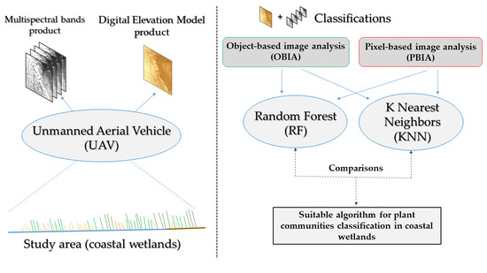
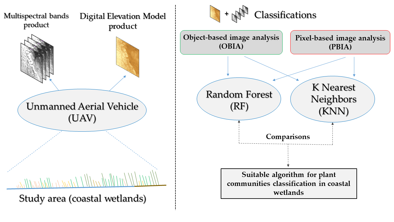
2. Materials and Methods
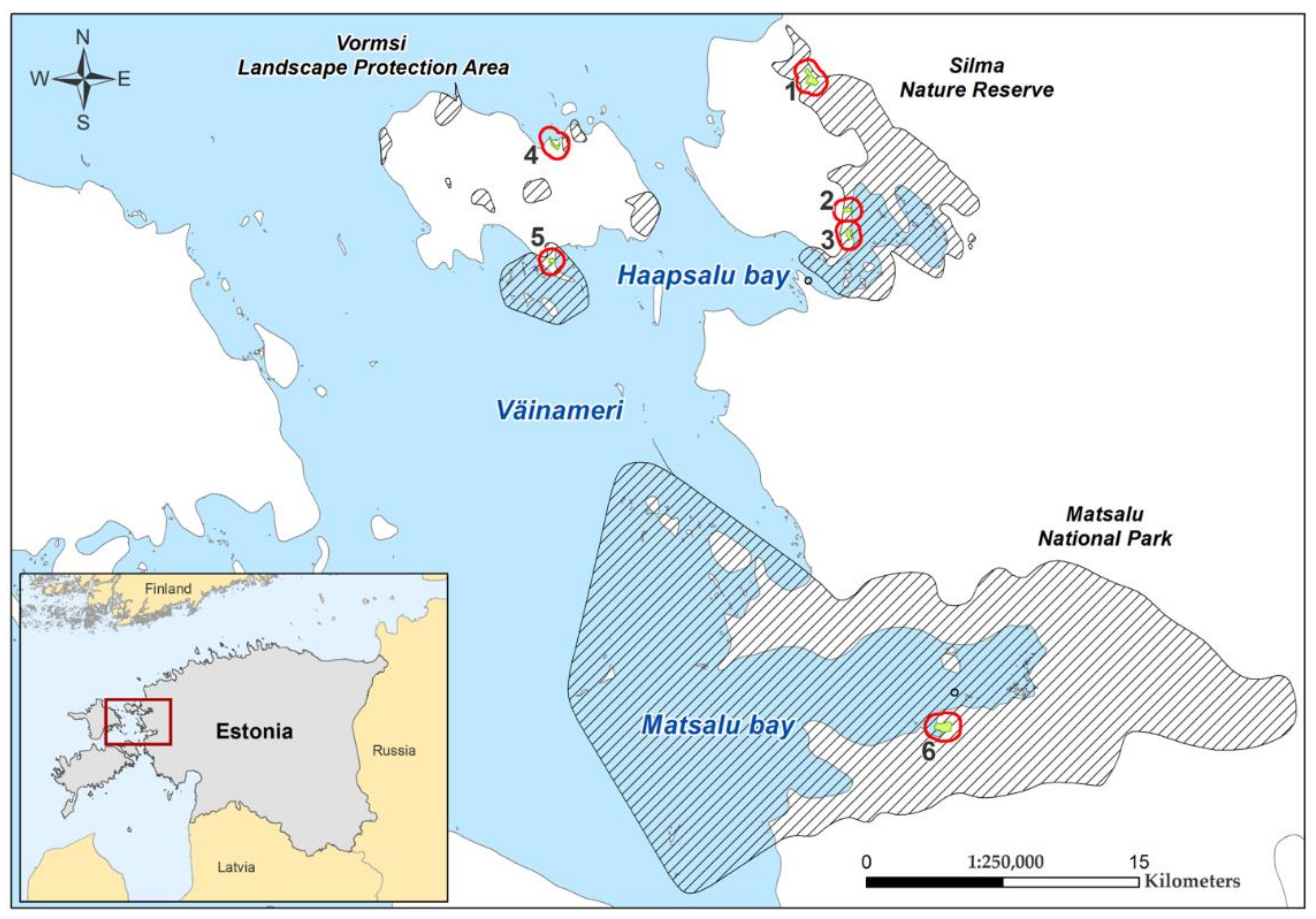
2.1. Study Areas

This study was undertaken in six coastal wet grasslands of Estonia, which belong to the classification ‘Boreal Baltic coastal meadows’ according to Annex I of the EU Habitats Directive (1992). These coastal wetlands are located in an extensive transitional zone from the sea to terrestrial ecosystems, characterized by a gradient of hydrological conditions and different inundation that largely determines the distribution of the plant communities [32,33]. Several studies have shown that microtopography also has an important influence on the location and extent of plant communities [34], including in Estonian coastal wetlands, where the total elevation differences are typically between 0 and 3 m, the tidal variation is negligible (0.02 m) and the range of plant communities is maintained through low-intensity grazing [35,36].
Figure 1 shows the location of the six study sites on the west coast of Estonia within nature protection areas and under low-intensity land management regimes [33,37]. Kudani (KUD), Tahu North (TAN) and Tahu South (TAS) are within the Silma Nature Reserve; Ralby (RAL) and Rumpo East (RUE) are within the Vormsi Landscape Protection Area; and Matsalu02 (MA2) is within the Matsalu National Park. The reason of choosing these study areas were due to the aim of classifying different structures of plant communities in coastal wetlands with different grades of heterogeneity and microtopography.
The study areas were digitalized manually, excluding the forests. The plant communities present in the study areas are categorized into five classes (Table 1) Table 1. Plant communities sampled in each study area, elevation range and area. LS: Lower Shore; OP: Open Pioneer; RS: Reed Swamp; TG: Tall Grassland; US: Upper Shore. according to Burnside et al. [38].

2.2. Data Collection

2.2.1. Field Sampling

Plant community sampling was carried out in June and July 2019 following the phytosociological classification developed by Burnside et al. [38]. Five plant communities (categories) were identified: Lower Shore (LS), Open Pioneer (OP), Reed Swamp (RS), Tall Grassland (TG) and Upper Shore (UP). As seen in Table 1, not all the plant community classes are present in all study areas. In total, 140 quadrats of 1 m2 were surveyed using a stratified random approach (ten quadrats per plant community at each site) [35]. The X, Y and Z coordinates of the plots were recorded within all quadrats using a Sokkia GSR2700 ISX differential global positioning system (dGPS). Points were recorded in the corners and center of all quadrats, five points per quadrat, as seen in Ward et al. [36]. This allowed us to record the location and elevation of the polygons for the training areas within each study site.

2.2.2. Image Acquisition

Two UAV flights were undertaken in each study site with an eBee Plus fixed wing drone, one with a Parrot Sequoia 1.2 megapixel monochromatic multi-spectral sensor, the other with a senseFly S.O.D.A. The Parrot Sequoia camera records data from four bands (Green 550 nm@40 nm, Red 660@40 nm, Red Edge 735@10 nm and Near Infrared 790@40 nm). The camera was calibrated prior to the flights using the Airinov calibration panel. In addition, this camera includes a sunshine sensor mounted on the top of the UAV to record sun irradiance for every shot. This retrieves the reflectance values on images. Flight heights were 120 m above mean sea level and the pixel resolution was 10 cm in all the images.
The flight using the photogrammetry camera senseFly S.O.D.A. reached a height of 123 m above sea level, recording RGB images at a resolution of 3.5 cm per pixel.
All flights were carried out during the summer period (Table 2), as inundation is minimal, so the presence of water does not substantially affect reflectance values of images [39] and the phenology provides optimal reflectance values [40].

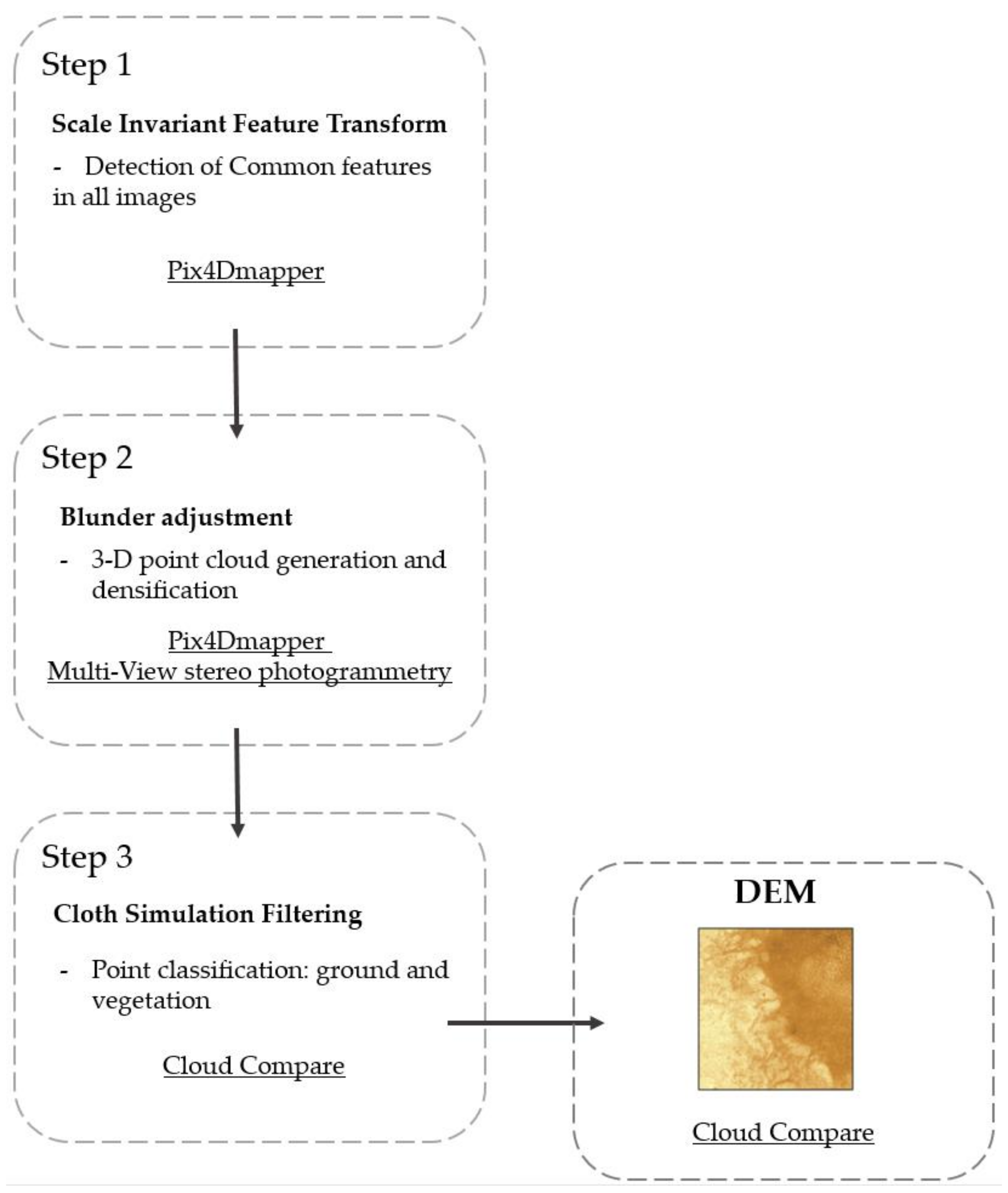
2.3. Image Processing

2.3.1. Positional Accuracy

RINEX observation and navigation files were used to carry out post-processed kinematic (PPK) correction of the multispectral images to improve the positional accuracy [41], using ESTPOS Estonian GNSS-RTK permanent stations network (Eesti Maa-amet) as a reference. There were 7615 images geographically positioned using the Estonian Coordinate System of 1997 (EPSG: 3301) and the PPK retrieved an accuracy value under 7 cm accuracy using the software eMotion 3®. The resulting orthomosaics were used as an input for the Pix4D v.4.3.31® software to obtain five orthomosaics per study area [42].
The accuracy of the PPK corrections was assessed using Root Mean Square Error (RMSE) and Mean Absolute Error (MAE) calculations. RMSE and MAE were used to estimate the differences between the ground control points (GCPs) location in the images and the independent GCPs locations measured with the dGPS [43]

2.3.2. Digital Elevation Models

The process known as Structure from Motion (SfM), described in Westaby et al. [13], is summarized in Figure 2. This process retrieves an accurate digital elevation model (DEM) that is able to represent the microtopographic elevation values that influence the distribution of plant communities [29].
The main objective of the SfM is to find matching locations in the multiple images to extract the photogrammetric points. Pix4Dmapper software is used with the Multi-View stereo photogrammetry module (SfM-MVS) to find common features within all the images [44], as seen in Step 1 (Figure 2). In Step 2, a bundler adjustment where a low-density point cloud was extracted from the common points using the view stereo photogrammetry, followed by its densification, where an enhanced 3D point cloud is built from different camera positions [44]. Finally, in Step 3, the point cloud is classified in two categories: ground and non-ground, using the cloth simulation filtering. This technique is based on the interaction between a cloth model and the inverted point cloud to select the shape of that cloth model [45]. This last process is computed in CloudCompare software. Only two parameters had to be set, the “rigidness” and the “ST”, in order to control how the cloth model lies over the inverted point cloud. The final DEM is extracted by performing an interpolation from the filtered point cloud (Figure 2). After processing, the RMSE was between 5 and 18 cm using the dGPS measurements.
Each DEM was resampled to the pixel size of the spectral bands in each study area, using the Nearest Neighbor method.

2.3.3. Vegetation Indices

Calculating vegetation indices from the original bands allows the retrieval of vegetation properties in the images by sharpening the differences of the spectral values of plants while avoiding interferences of soil and vegetation components without a photosynthetic response [46]. Furthermore, the vegetation indices have been shown to be reliable for monitoring and detecting types of vegetation due to their correlation to biophysical properties in plants [47,48]. We calculated ten vegetation indices (Table 3), which were used as input images for the segmentation and classification processes, as they can improve the classification accuracy [46].
We performed band calculations to obtain the vegetation indices using the open source software R (v4.03) [49] with the packages raster [50] and rgdal [51].
The indices in Table 3 have been shown to be sensitive to the chlorophyll content in different scenarios where plant and soil structures interact with the reflection of leaves as well as differentiating plant species. Additionally, the red edge band is more sensitive to chlorophyll and the presence of water, and may discriminate the plant communities according to their wetness [62].

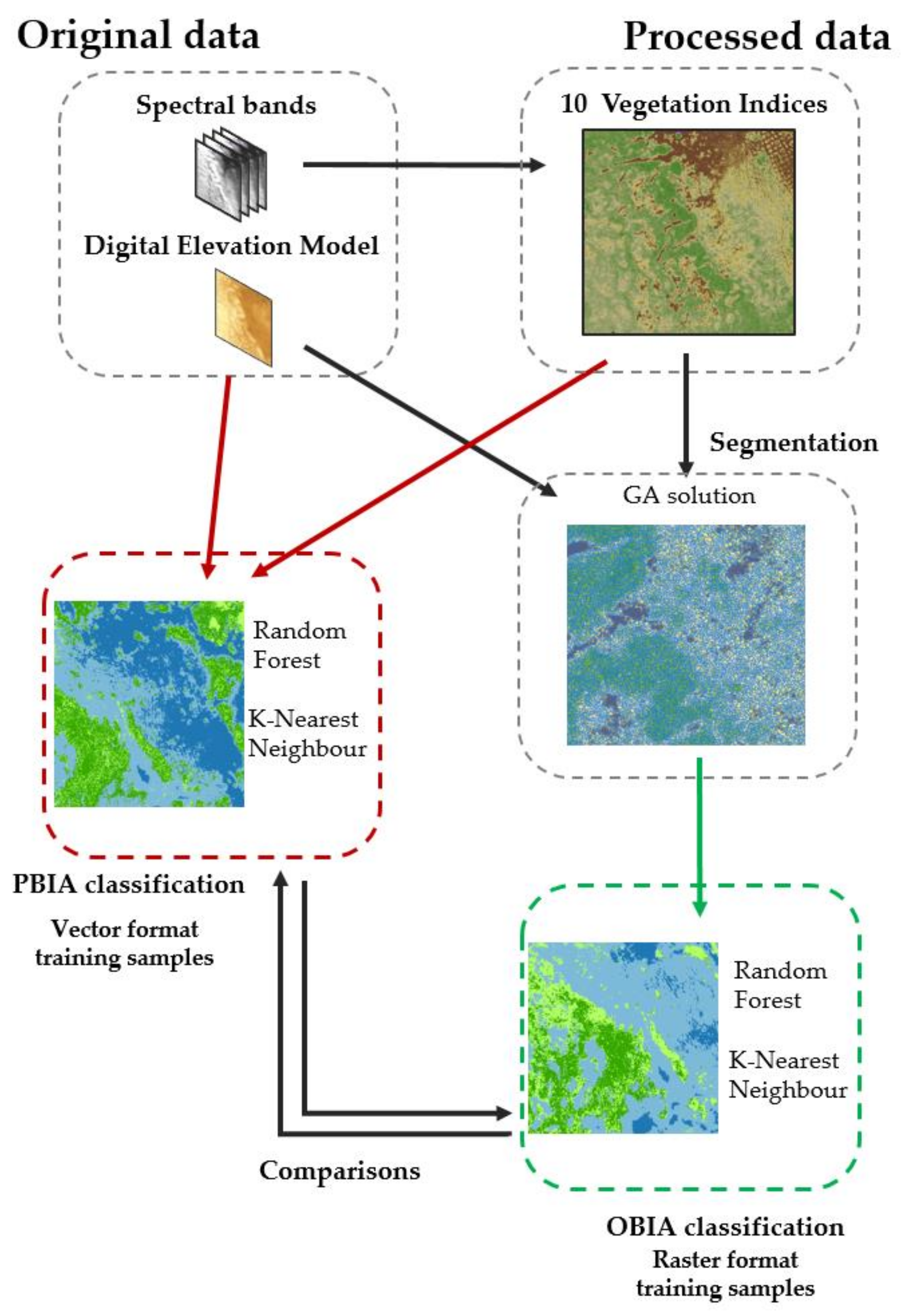
2.4. Classification of Images

We performed an image classification using two different approaches: Pixel-Based Image Analysis (PBIA) and Object-Based Image Analysis (OBIA). The former has been used in since the first Landsat satellite took the first remotely sensed images, where coarse spatial resolution images are classified, and a single pixel is big enough to represent an object of interest. With the recent increasing resolution of satellite images and the use of UAV to record high-resolution images, single pixels may not always represent meaningful units, but a group of pixels as objects can do so. In OBIA, an image segmentation is performed to create a homogeneous group of pixels [63] and represent the objects for classification. In supervised classifications, an unknown sample (pixel or object) is assigned to a class based on an original training dataset, from an n-dimensional space (feature space) of explanatory variables. These variables are the bands extracted from spectral measurements, combinations of them or ancillary geographical data [64].
Figure 3 shows the workflow to classify the images using the PBIA and OBIA approaches.

2.4.1. Segmentation

In the OBIA approach, image segmentation is the first step to create objects for classification. The segments are discrete units of spatial entities composed of homogeneous values in a multidimensional feature space [26]. In order to obtain optimal segmentation parameters for a considerable classification accuracy, previous studies have justified their choices based on trial-and-error approaches and visualizations [27]. Instead of following this process, we chose to use a Genetic Algorithm (GA) (Figure 3). This type of algorithm imitates the evolutionary process to obtain a fitness function, which finds the optimal solution to solve a complex computational problem [65]. It has been shown that the Genetic Algorithms improve the classification accuracy for a large number of variables (bands) [66].
To carry out the segmentation of images, we chose the SegOptim package written in R [67]. This package integrates a complete workflow for segmentation and classification of images. First, the R package uses the functions of third-party software to perform the image segmentation after tuning the parameters for the segmentation by applying a GA.
In this study, we chose the Large-scale Mean-shift algorithm [68] for the following reasons: it is executed in SegOptim by calling the Orfeo Toolbox library [69], (also open-source software); the tuning parameters consist of setting the spectral and the spatial range of pixels in the feature space and establishes the minimum size of the segments; it performs a stable and efficient segmentation of images as it splits the image into tiles. The Spectral Range indicates the search radius in multispectral space; Spatial Range, the similarity of neighbors; and the minimum size of segments in pixel units.
The input variables for the GA were the vegetation indices (Table 3), the DEM and the training samples. The training samples, originally in vector format, were rasterized, as SegOptim only accepts the training samples as a grid of category values. The mean size of the training areas in the raster format was 11 pixels. Each raster is then assigned to the segment based on a threshold value. Due to the small size of the training areas, this threshold was set to 5%, meaning that the segments covered by 5% or more by the training pixels were considered as valid cases for the classification, characterized by the mean and standard deviation of the values of variables [55].
Finally, the fitness value in SegOptim retrieved the best parameters to apply to the segmentation in each study area for the following classification using RF or KNN. The result was a segmented image in raster format (Figure 3).
In order to see if there were differences between the training areas as segments (valid cases for training the classifiers) and polygon features, we compared the mean values of each variable (input vegetation indices and DEM). To do so, we carried out a Kruskal–Wallis non-parametric test between the medians of the training samples and segments with the characteristics of the training samples in each plant community because the values did not follow a normal distribution.

2.4.2. ML Classifiers

To perform a PBIA and an OBIA, we chose the RF and KNN classifiers (Figure 3).
RF is a nonparametric ensemble classifier (multiple classifications on the same data) that grows multiple decision trees from a subset of training samples with replacement (bagging) [70]. The group of trees make a final decision based on the most repeated vote (modal category) and label the final category to an unknown sample. While the forest is being built, the samples not used for training are the out of bag (OOB) fraction, which estimates the internal performance with an error rate [70]. This OOB is also used in the calculation of the variable importance by randomly replacing one input variable in the out of bag fraction by another variable randomly selected. If there is an increase in the OOB error, the variable was important to reduce the error, and thus, it is considered more important in the tree [71].
The KNN algorithm is a nonparametric classifier, which assigns a class label to an unknown sample based on its statistical distance to the training samples. The Euclidean distance is used by default in the caret package applying the KNN method. Once the distance is calculated, it selects the K-Nearest Neighbors to assign the modal category in those k training samples. We searched for the best accuracy between 1 and 20 K-Nearest Neighbors. These minimum and maximum k values were set initially between 1 and 26, as this resulted from the average k of all the study areas after calculating the square root of n (n = number of pixels in training samples) [72]. However, in all cases, after k = 20, the accuracy decreased.
For a PBIA classification, we used the caret package [73], which can perform an RF and KNN classification by changing the arguments in the required functions (method = “rf” or “knn”, respectively). This function requires the input variables in grid format to be stacked in a multiband raster and use the training areas as vector format (polygons).
For the OBIA classification, the output segmentation obtained in the previous step was used to classify the objects. Prior to classification, a calibration phase was undertaken, where the category values of the training samples are assigned to the segments containing those pixels, based on a threshold value. This classification, as mentioned before, was carried out using the SegOptim package.
We carried out four classifications in each study area: RF and KNN based on PBIA and RF and KNN based on OBIA.

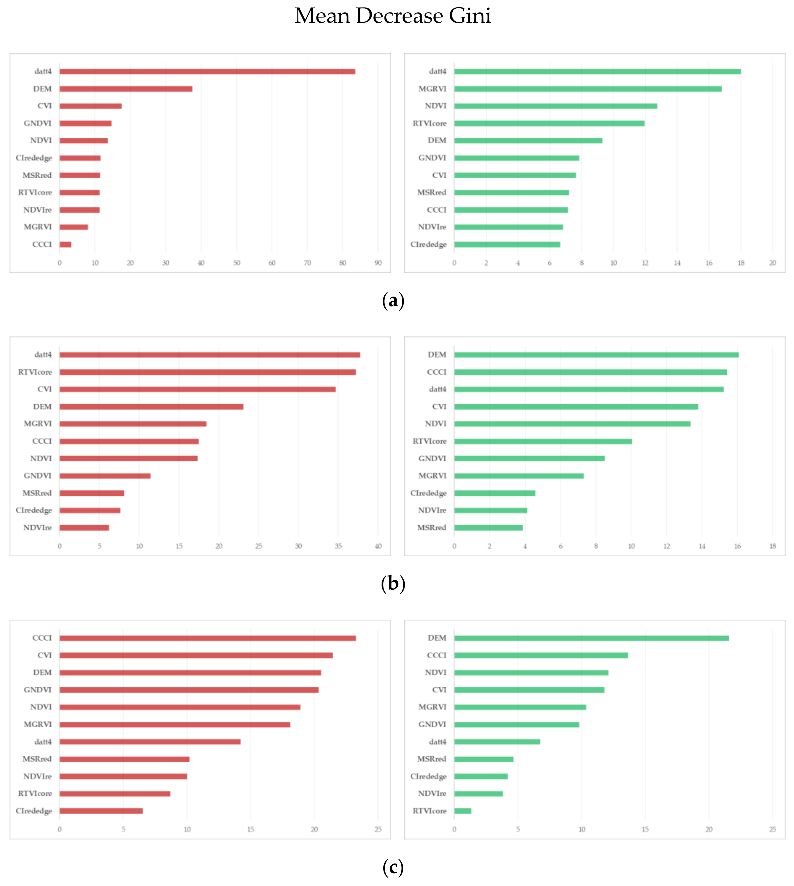
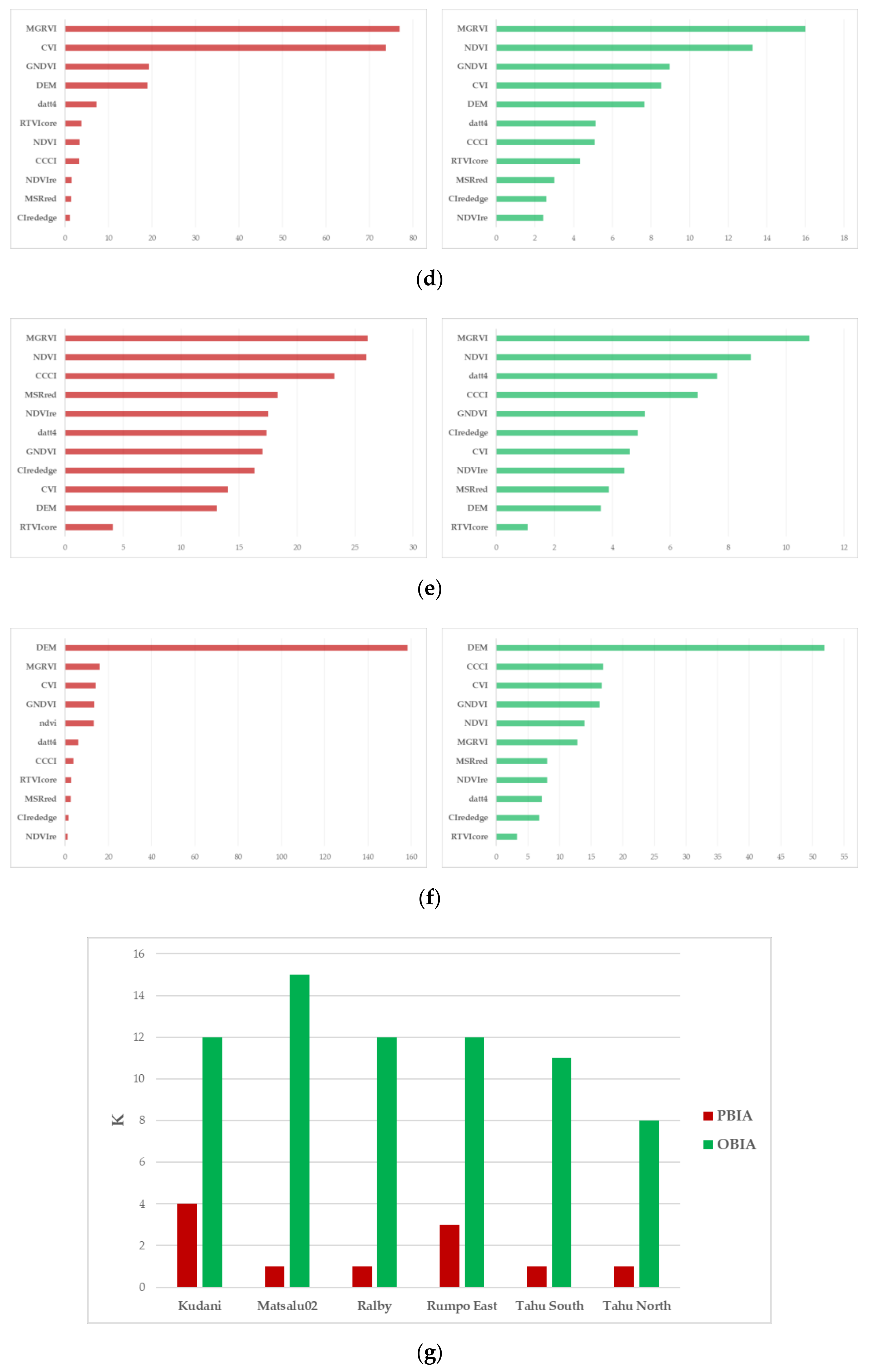
2.4.3. Classification Accuracy and Variable Importance

We consider the accuracy as the agreement between a classified value previously unknown and the training samples, accepted as true values [74]. The classifications were evaluated using the User accuracy, Producer accuracy, overall accuracy and Kappa statistic with a 10-fold cross-validation to construct the confusion matrices for each classification. For RF classification based on PBIA and OBIA, we extracted the Mean Decrease Gini (MDG) to report the variable importance in each study area. The MDG is based on the Gini impurity criterion, which calculates the chance to misclassify a new sample. Replacing the purest variable in a node with another one will increase the chance to classify incorrectly the new sample, so that the previous variable was more important (pure) to split the node [25]. The higher the MDG is, the more important the variable is.

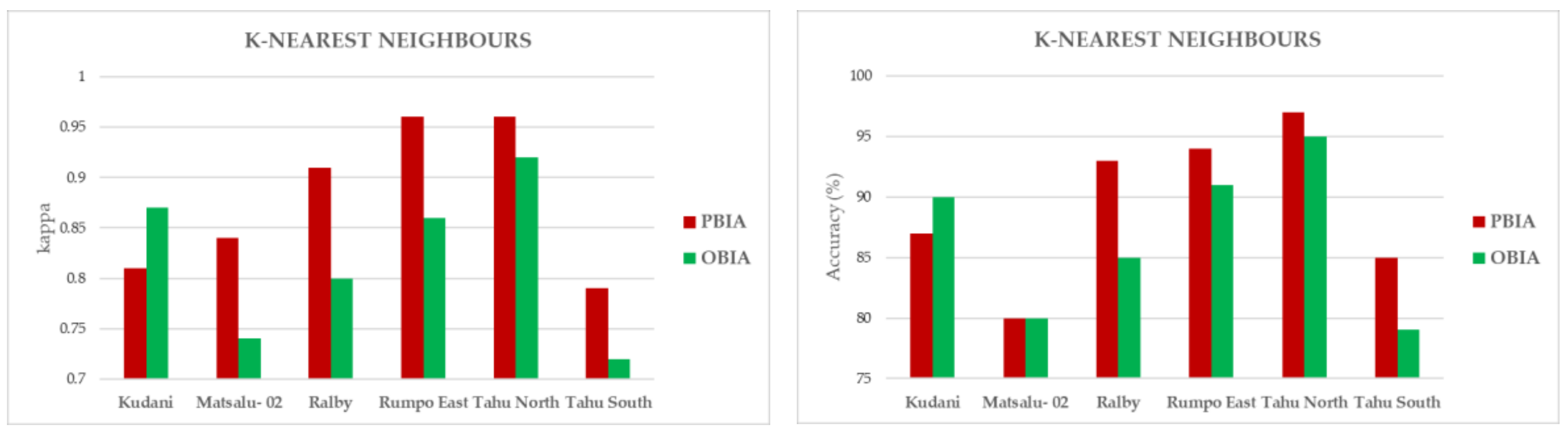
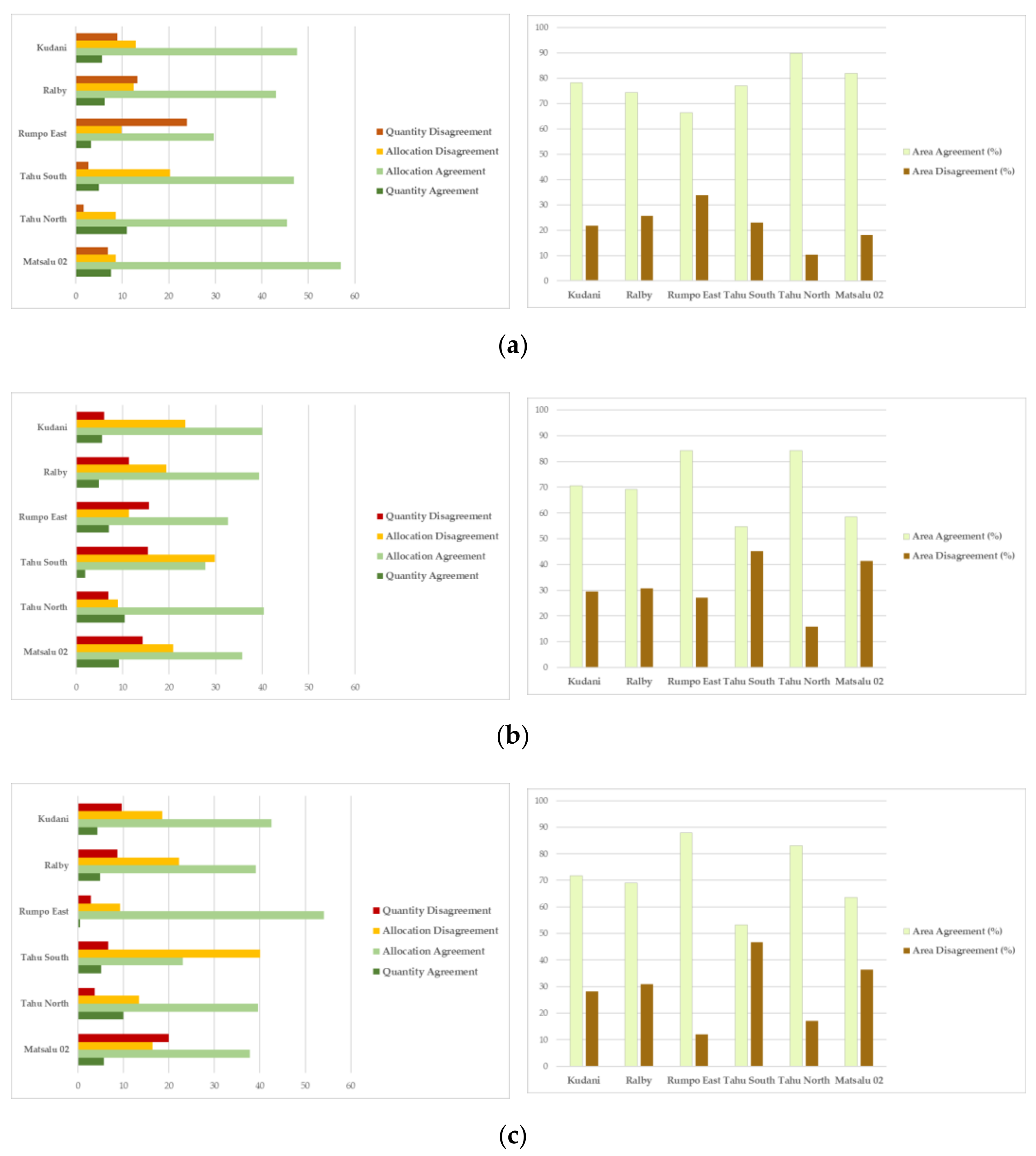
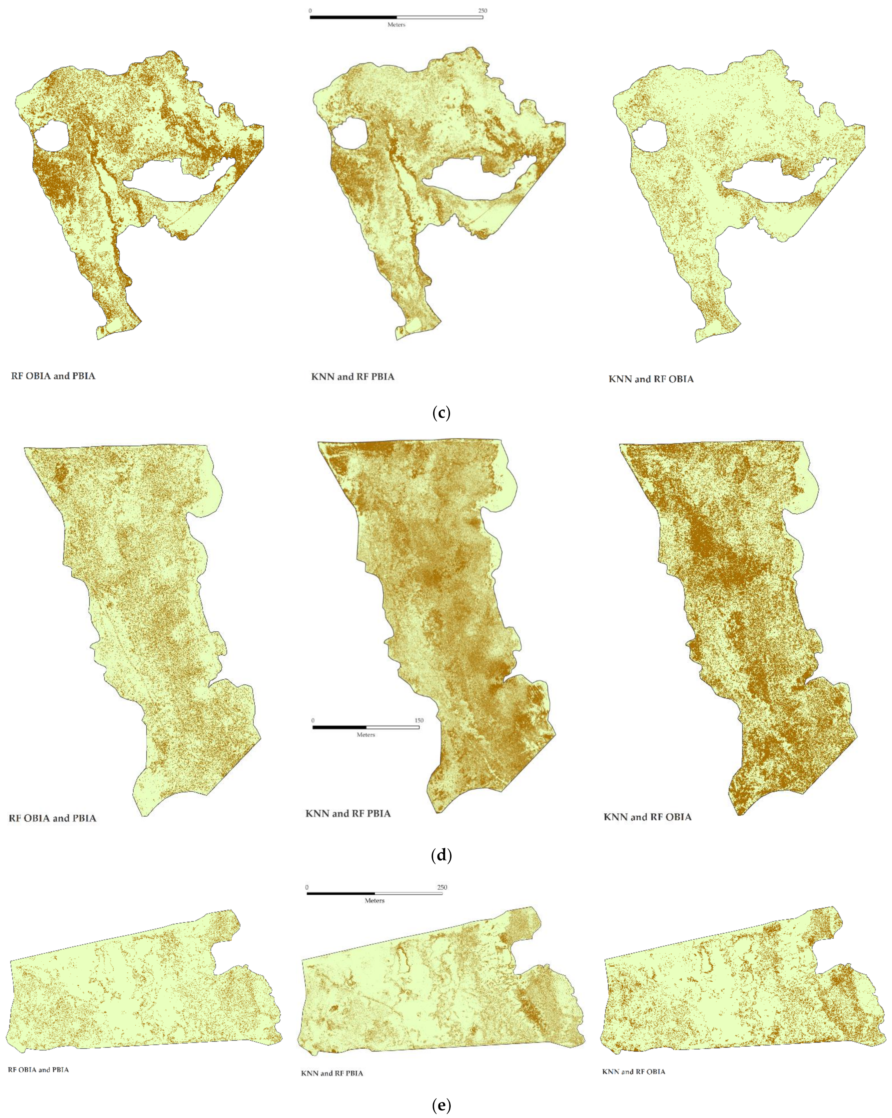
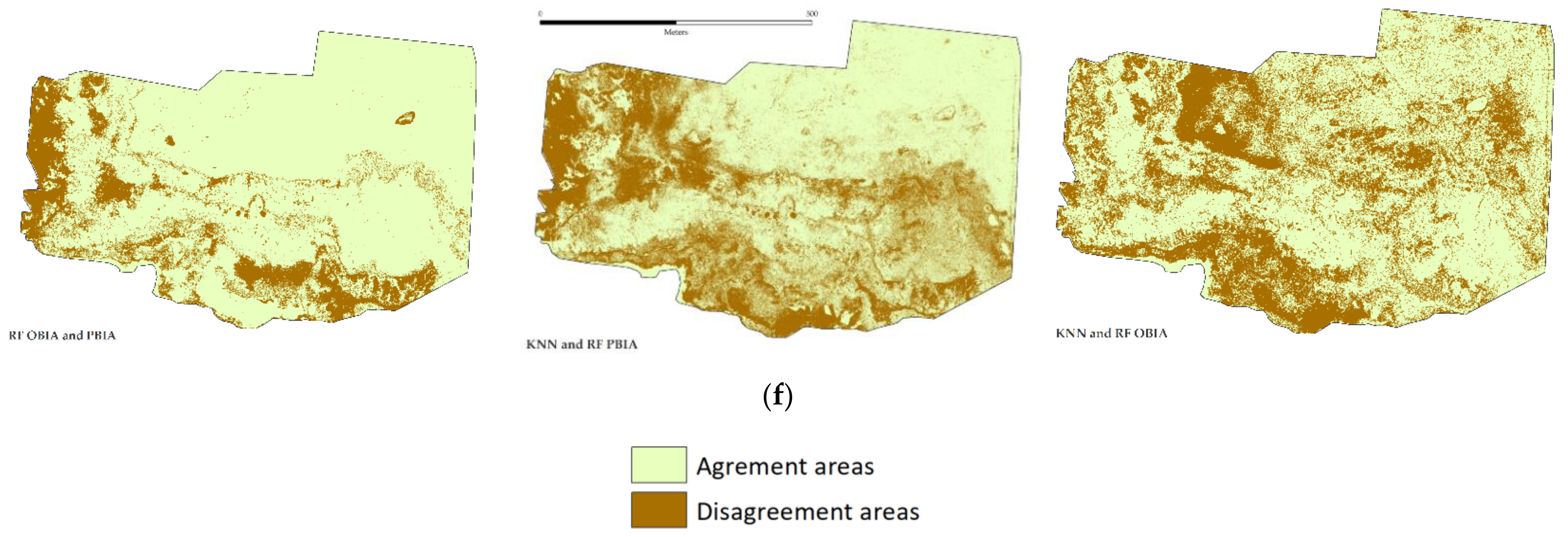
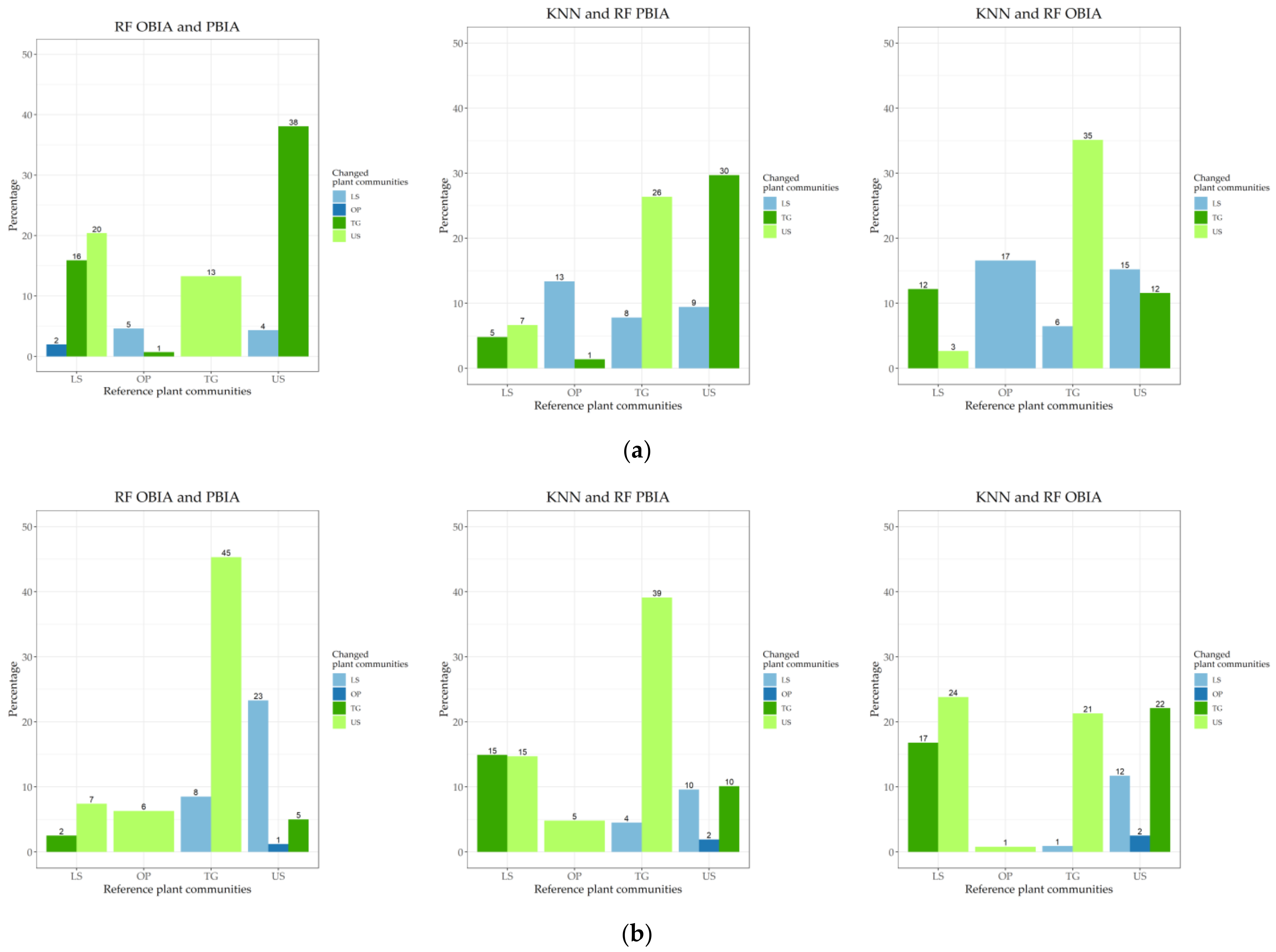
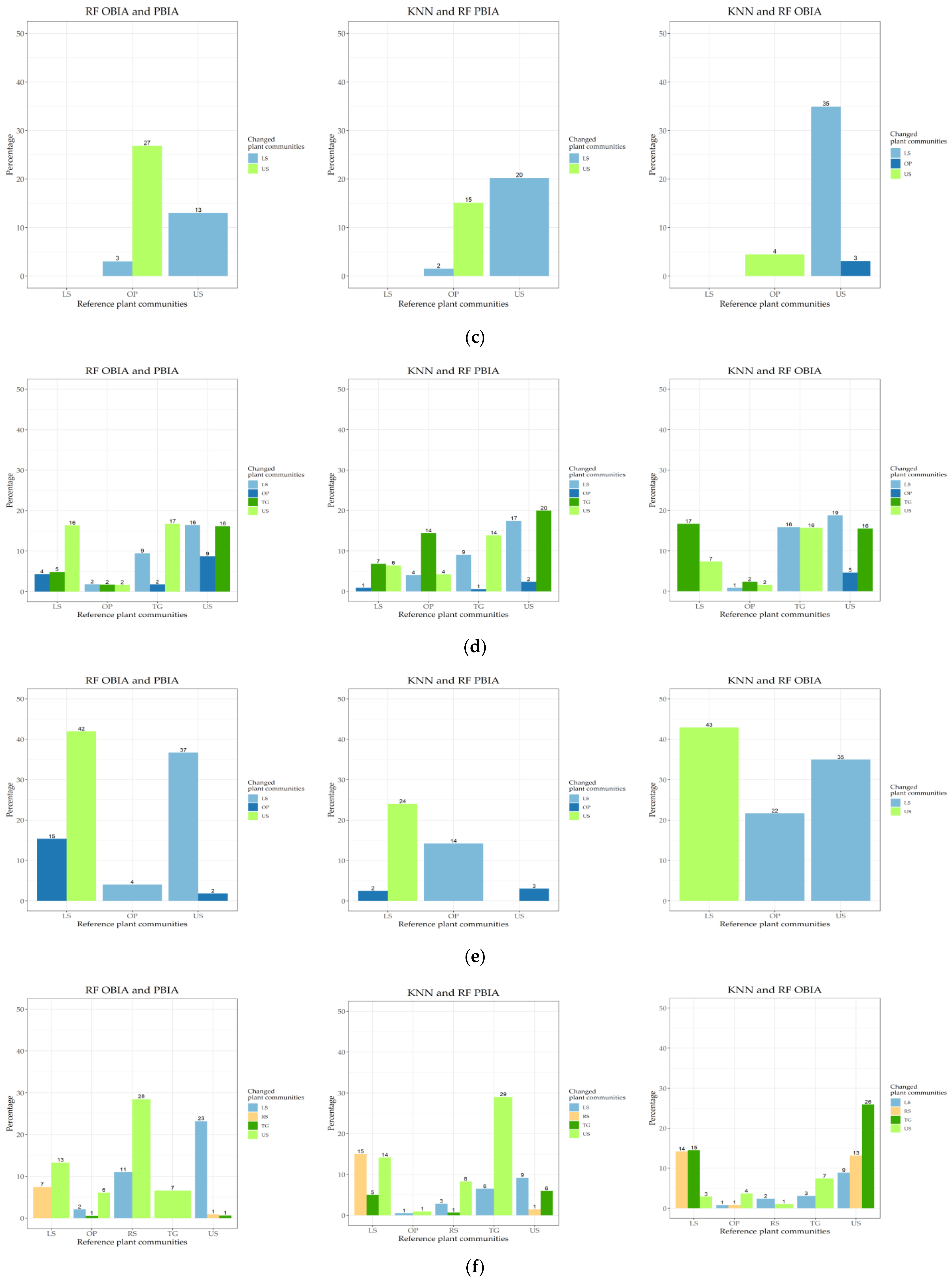
2.5. Map Comparisons

A common task in remote sensing is to perform a comparison between classifications in order to assess the differences in thematic maps [75]. Despite the widely used parameters derived from kappa statistics to compare categorical maps [76,77], called Khisto, Klocation and Kquantity, these parameters are not sufficient to compare accuracies as they have a randomness component [78]. To overcome these limitations, within this study, a new measure of overall agreement is used as a simpler measurement. It is composed of two metrics, quantity and allocation disagreement. The first component refers to the proportion of differences of unmatching categories and the second one to the differences due to the displacement of categories in the area [78]. These comparisons are performed between maps with the same pixel size.
The ML algorithm with the highest classification accuracy was chosen as the reference map. Comparisons were performed between PBIA and OBIA of the best classifier. We reported the percentage of agreement and disagreement areas between maps and the overall percentages of quantity and allocation agreement and disagreement relative to each study area using the Rsenal [79] package in R software [49]. The variation in the quantity of each category (plant communities) refers to the differences in their composition throughout the area and the variation in allocation, to the differences in their spatial configuration [80]. This allowed the interpretation, in a spatial context, of the differences among the classifications. We also calculated the changes of categories within the disagreement areas.
The remaining percentage (the sum of quantity and allocation agreement and disagreement is not 100%) corresponds to the proportion of agreement that is expected to occur by chance (chance agreement).

3. Results

3.1. Segmentation and Comparison between Training Areas

The GA retrieved the best solution between given maximum and minimum values for each classifier as shown in Table 4. This creates segments according to a search radius based on these values. On average, the size of the training samples in RUE, KUD and RAL are 8 pixels per quadrat, 9 in MA2 and 5 in TAS and TAN, although the category of OP has larger training areas in TAS, TAN and RUE, which are 21, 40 and 42, respectively. The Kruskal–Wallis test did not show any differences between these segments and the initial training polygons.

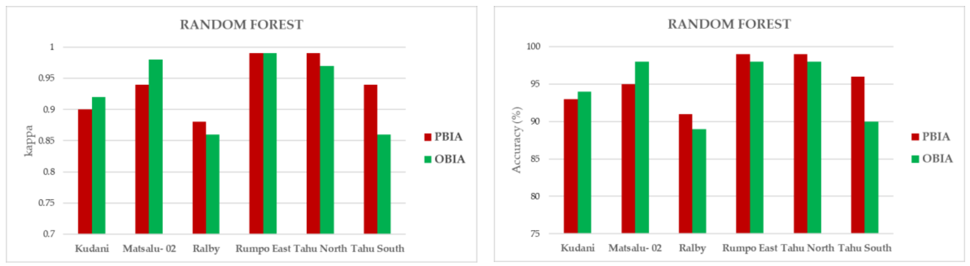
3.2. ML Accuracy Assesment

Figure 4 shows the kappa indices and accuracy scores of the classifications obtained in each study area. The kappa statistic in all the classifiers was greater than 0.7, far from a random classification, and all accuracies reached at least 80%, except the KNN classifier in TAS using OBIA (Figure 4). The classified maps are shown in Figure A1. PBIA approach generally performed better than OBIA and RF algorithm performed better than the KNN algorithm. KUD and MA2 are the only two sites where the OBIA approach performs better than PBIA using the RF algorithm and KUD with KNN algorithm (Figure 4).
According to the MDG, the study areas of KUD and MA2 have only one important variable in common (datt4 and DEM respectively) to build the RF classification model (Figure 5). The first eight variables that are more important in the RF classification using PBIA and OBIA are DEM, CVI, MGRVI, Datt4, CCCI, NDVI, GNDVI and RTVIcore (Figure 5).
The number of nearest neighbors (k) is higher in OBIA (Figure 5), probably due to the more homogeneous characteristics of the segments, which is why the classifier chose a larger distance for the training samples than in PBIA.

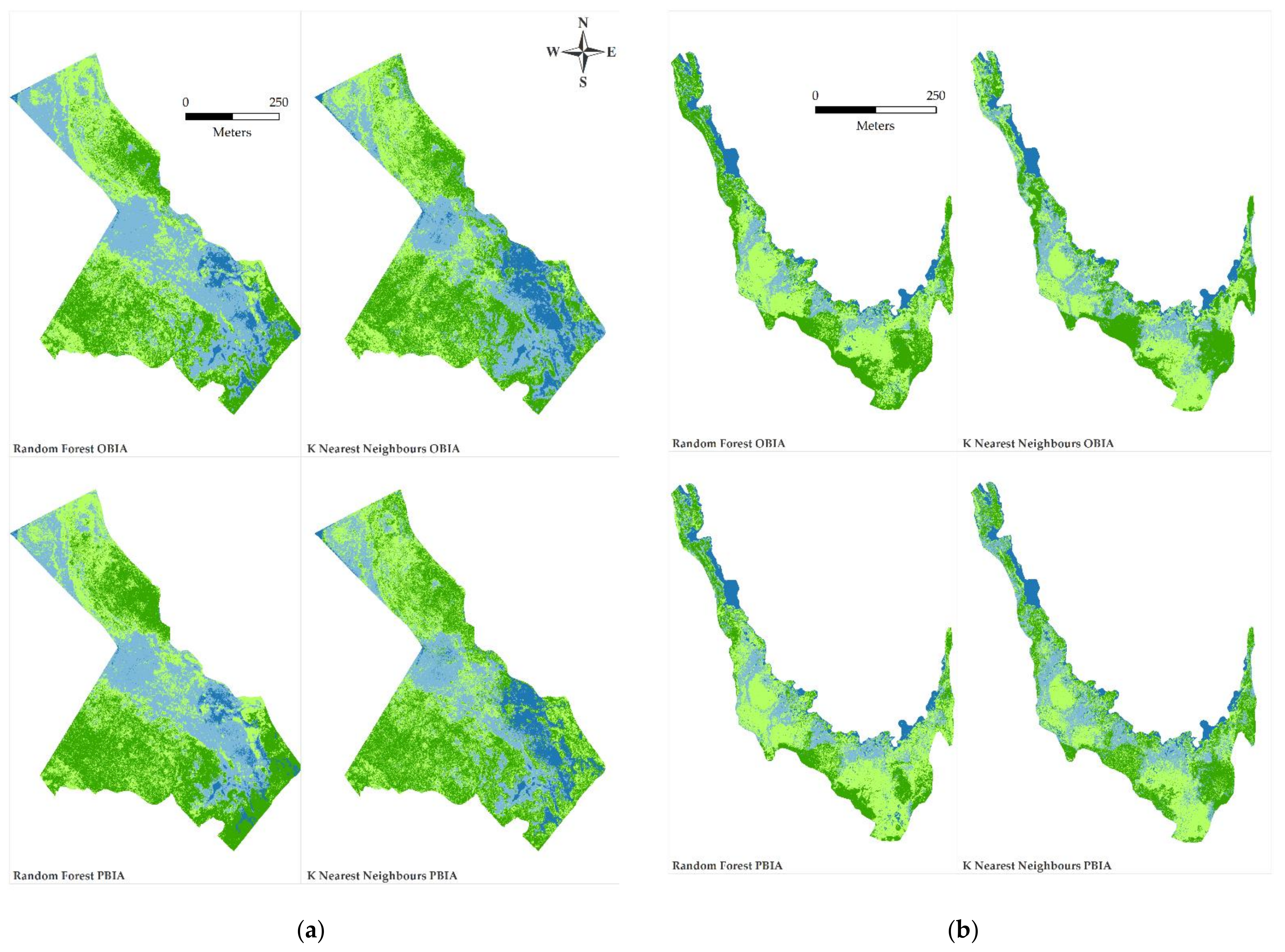
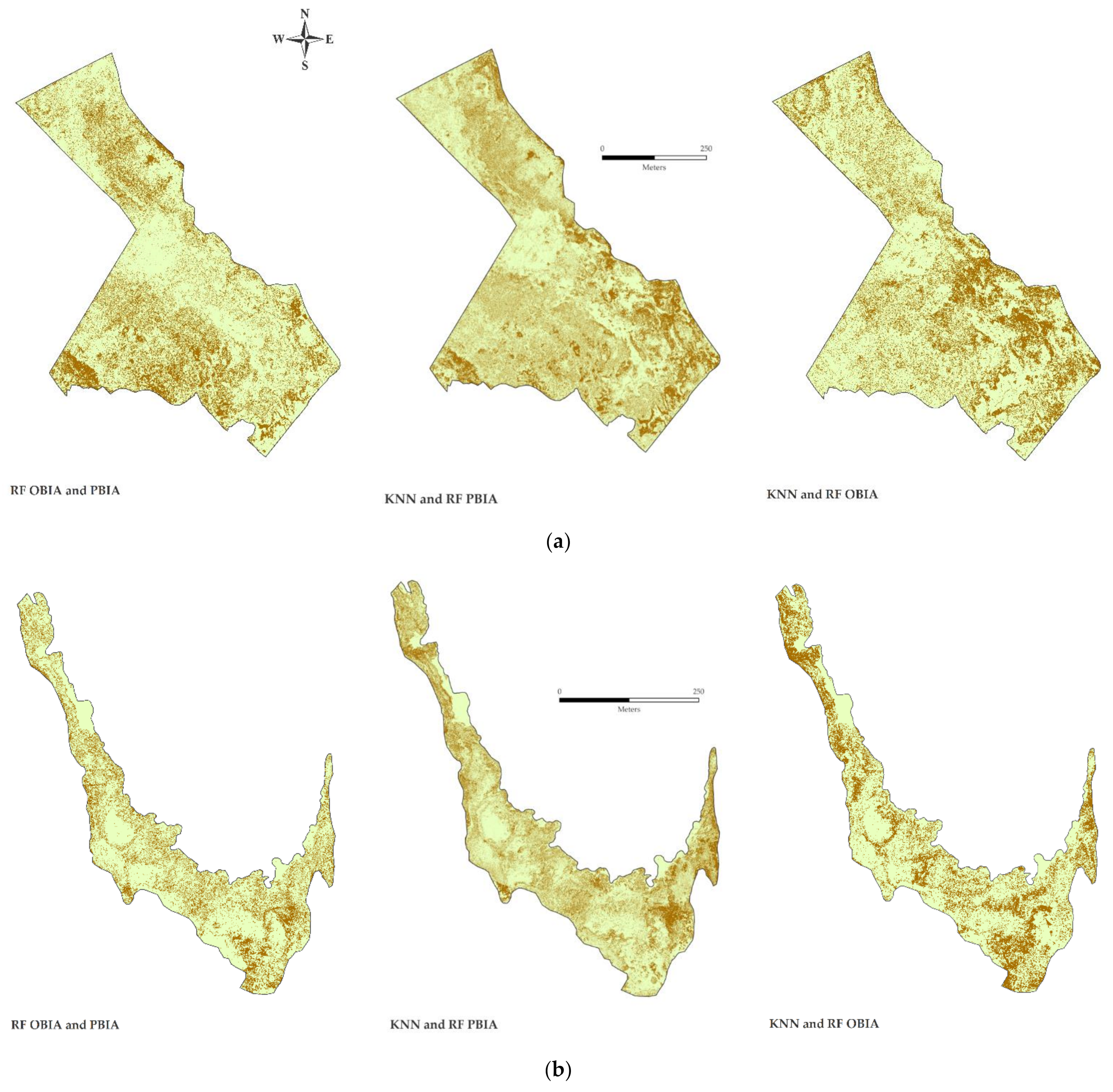
3.3. Map Comparisons

As RF was the most accurate classifier, we used it as the reference for the comparisons.
The highest agreement between classifications is the RF classification OBIA and PBIA, where the areas of agreement are greater than 65% of the total area (Figure 6). This means that RF has classified the images in a way that pixels follow similar patterns to the segments. In the classified maps of RF using OBIA and PBIA, both maps have a similar spatial configuration (Figure A1). Nevertheless, the quantity of categories is different, mainly due to the difference of category OP to US, which represents 27% of the area of disagreement. On the contrary, the site TAS has the highest allocation disagreement in relation to the quantity disagreement (Figure 6).
The categories that were mixed in the disagreement areas in the study areas the most were: KUD (38% from US to TG), RAL (45% from TG to US), RUE (27% from OP to US) and TAN (42% from LS to US and 37% from US to LS). In TAS and MA2, the mixture is due to more than two categories (Figure 6).
The RF and KNN PBIA classifications exhibited the greatest extent of disagreement areas. In this instance, the main changes were between the categories of TG and US, except in TAN, where changes were between LS and US. Allocation was generally higher than the quantification disagreement between these two classifiers. The agreement areas between RF and KNN OBIA is better than the PBIA, possibly because pixels and segments share the same area in both classifications (Figure 6).

4. Discussion

The use of high-resolution images to classify plant communities in wetlands has been previously undertaken in several studies using either commercial satellites (<4 m resolution) [81,82,83] or UAVs images (<0.1 m resolution) for environmental assessment [10,84]. Classification of plant communities in coastal wetlands, where individual plants are less than 1 m wide (e.g., coastal grasslands, floodplain grasslands, saltmarshes and seagrasses) benefits from the use of very high resolution data to reveal as much spectral variability as possible [38,42].
The use of ML algorithms in remote sensing has provided a solution for complex classifications, using additional explanatory variables apart from spectral values to build classification models, such as vegetation indices or DEMs [22,42,84]. These algorithms can also classify categorical units in a more complex feature space, where the spectral separability is low due to the higher variability within classes [85].
Classification using the RF algorithm was better than KNN, both in PBIA and OBIA, in all the study areas except in RAL, where KNN using PBIA showed a higher accuracy and kappa index (Figure 4). These results show that using ML algorithms is appropriate for these types of images, but RF produces more robust results than KNN in coastal wetland plant communities. The reason is that RF builds a classification model using different response variables and extracts the variable importance based on the OOB error from a bagging method to assess the main contribution of each variable [22,71,86,87]. The KNN classifier, while a robust algorithm [24,88], does not perform so well in complex feature spaces while calculating the nearest neighbors [22,89]. This explains the larger areas of disagreement when KNN and RF classifications are compared (Figure 6). The outputs of distribution areas in the RF classifier match the complex mosaic of plant communities observed on-site, due to transitions from one plant community to another, disturbances or restoration activities (Figure A2). The comparison between OBIA and PBIA in RF shows that disagreement areas are also located in heterogeneous locations where segments do not represent the heterogeneity of the plant communities. The disagreement areas are due to a different spatial configuration of the categorized plant communities and to the “salt and pepper” effect, as described in high-resolution image classification [27].
According to the variables used, the MDG results from RF classifications show that the most repeated important variables in both approaches are the DEM, MGRVI and CVI (Figure 5). As shown in the literature, microtopography significantly influences the distribution of plant communities in coastal wetlands [2,29]. On the other hand, the two vegetation indices are shown to have a high potential discrimination in the RGB spectrum (MGRVI [61]) and in the NIR spectrum (CVI [54]) related to leaf chlorophyll content.
Selecting the most suitable segmentation for an OBIA classification can be a complex task due to the low spectral contrast between plant species in coastal wetlands [90]. In this study, we tried to avoid this problem by using a GA (Figure 3), as this selects the best parameters to provide the most accurate classification (Table 4). In addition, we used the DEM and vegetation indices instead of spectral bands, as they enhance differences between plant communities [42,46] for segmentations and classifications. The segments required a low variability of input bands as explanatory variables (“spectral range” as parameter) and size parameters to extract meaningful units similar to the training samples. Therefore, the segments used for training do not differ significantly from the original training samples. This was because we plotted small samples in the field in order to get the purest training samples. Nevertheless, this was suitable to obtain high accuracy classifications with an OBIA approach.
PBIA performed better than the OBIA classification in most of the study areas except for KUD and MA2 in the RF classifier and KUD in the KNN classifier (Figure 4). In these areas, there are greater cattle grazing pressures (though still at a low intensity) in than the other sites [37], which may create larger patches of homogeneous plant communities in terms of the reflectance response. In this instance, the segments would have grouped pixels that are more homogeneous, in part explaining the marginally better performance of the OBIA classification in this site. Nevertheless, this is not the case for MA2. This area has a homogeneous distribution of plant communities, clearly influenced by the limited variation in elevation. Unlike KUD, MA2 objects are mixed together. The results in panel g of Figure 5 show the use of a greater number of neighbors in the KNN classifier using the OBIA approach than in the PBIA approach, due to the need of longer statistical distances between categories to classify the segments.
There are disagreements between the classifiers due to similarities in the plant communities, mainly LS, TG and US (Figure A3). These categories of plant communities belong to a broader grassland classification [38], where the spectral values might be similar in spite of the influence of the microtopography (DEM). This study does not look for the reasons why these differences occur from a physiological perspective and the authors suggest further research using different band combinations in order to retrieve different vegetation indices and to see if this also occurs in ecotones of different ecosystems.
Most studies suggest that the use of OBIA extracts the meaningful spectral information of images by reducing the “salt and pepper” effect after classifying high-resolution images and also considers the spectral and spatial information of features when grouped into objects after a segmentation [27,63]. Nevertheless, classification accuracies using an OBIA approach depend on the spectral properties and their sizes according to the research goals [81]. This study shows better results with pixel classification (PBIA). A previous work chose the use of PBIA rather than OBIA for classifying high-resolution images taken from UAV in coastal wetlands, because its performance could decrease the spectral variability in the images [42]. Further work could prove lower classification accuracies by increasing the sizes of the training areas and, thus, the segments, as they homogenize larger areas.
It is important to note that uncertainties generated during the image processing are not addressed in this paper. However, it should be appreciated that the plant communities studied describe a gradient of change, not discrete units as seen in the classifications (Figure A1); thus, this is one important source of uncertainty. In addition, the extraction and resampling of DEM to the original spectral bands, the calculation of indices and the algorithms themselves are also a source of uncertainty that may affect the reliability of our classifications [91].
After using ML classifiers, we obtained accurate results for categorizing the plant communities in a heterogeneous area within different study areas. Therefore, we recommend their use for characterizing the vegetation structure not only in coastal wetlands but in similar ecosystems with mosaic patches of plant communities, including small plants, such as grasses, forbs, tidal grasslands and floodplains. PBIA classifications are better in situations when the vegetation cannot be grouped into meaningful objects. Further work needs to be done to show that OBIA really decreases accuracy as the sizes of training areas and, thus, the segments increase in coastal wetlands and ecosystems with similar characteristics where vegetation is highly heterogeneous.
According to our results, RF provides a robust and highly accurate classifier as well as working well with small training samples. RF also provides the variable importance scores that allow us to know which variable contributes to a better classification. This will help future research to study changes in plant community composition over time using the most important variables for categorizing vegetation. The possibility of carrying out near-real-time monitoring routines with UAVs allows us to acquire images over different periods and to classify them with a robust classifier such as Random Forest for producing thematic maps [42].
Performing a rapid mapping assessment of vegetation is essential to provide quick decisions in environmental management and conservation. The use of a rapid methodology to obtain high-resolution images and their classification using Machine Learning algorithms retrieves high accuracies, which can be used to monitor environmental changes over time and to compare different sites at the same time if we keep parameters constant for the classification and image acquisition. Further studies could use more training samples and categories to see whether the classifications of wetlands decrease due to a more complex feature space of the values in a pixel-based approach. In addition, the spatial variability of categories at the present scale of study could be compared to smaller scales using satellite-mounted sensors to perform upscaling of the images.

5. Conclusions

The use of ML algorithms is valuable to classify high-resolution images when the composition of study areas is complex. In this study, we have shown that RF and KNN classifications are accurate and robust when using vegetation indices and digital elevation models, but RF retrieved better results when classifying plant communities in coastal wetlands. In spite of the high accuracies in both PBIA and OBIA classifications, our results show that object-based classifications perform slightly worse than pixel-based approaches, because these ecosystems exhibit a high variability when using high-resolution images and grouping pixels masks some of that variability. PBIA is more suitable for classifying high-resolution images in coastal wetlands, where the goal is to show the variability in the study area. It could be useful to use OBIA as a post-process, such as generalizing plant community patterns or when larger training samples are available, allowing us to perform a segmentation using higher thresholds.
As shown in Figure 6, RF retrieves lower scores of disagreement between pixel and object classifications. Nevertheless, this depends on the study area and similarities between plant communities. It would be possible to improve the agreement between the RF classification of objects and pixels using images taken in flights from other dates or using other vegetation indices to discriminate other plant characteristics than those used in this study.

Author Contributions

Conceptualization, R.M.P., M.V.P. and R.D.W.; methodology, R.M.P., C.B.J., M.V.P., T.F.B. and R.D.W.; software, R.M.P. and M.V.P.; validation, R.M.P., M.V.P. and R.D.W.; formal analysis, R.M.P.; investigation, R.M.P., M.V.P., T.F.B., C.B.J. and R.D.W.; resources, R.D.W. and K.S.; data curation, R.M.P., M.V.P. and R.D.W.; writing—original draft preparation, R.M.P., M.V.P. and R.D.W.; writing—review and editing, R.M.P., M.V.P., R.D.W. and C.B.J.; visualization, R.M.P.; supervision, M.V.P., R.D.W. and K.S.; project administration, R.D.W. and K.S.; funding acquisition, R.D.W. and K.S. All authors have read and agreed to the published version of the manuscript.

Funding

This research was funded by the Doctoral School of Earth Sciences and Ecology, financed by the European Union, European Regional Development Fund (Estonian University of Life Sciences ASTRA project “Value-chain based bio-economy”).

Institutional Review Board Statement

Not applicable.

Informed Consent Statement

Not applicable.

Conflicts of Interest

The authors declare no conflict of interest. The funders had no role in the design of the study; in the collection, analyses or interpretation of data; in the writing of the manuscript, or in the decision to publish the results.

Appendix A

Figure A1. Plant community classification for each study area with the legend (below all the maps). (a) Kudani, (b) Ralby, (c) Rumpo East, (d) Tahu South, (e) Tahu North and (f) Matsalu02.
Remotesensing 13 03669 g0a1aRemotesensing 13 03669 g0a1b
Figure A2. Distribution and extent of agreement and disagreement areas per study area. (a) Kudani, (b) Ralby, (c) Rumpo East, (d) Tahu South, (e) Tahu North and (f) Matsalu02. From left to right: changes in RF in OBIA and PBIA classification; changes in KNN and RF in PBIA classification; and changes in KNN and RF in OBIA classification.
Remotesensing 13 03669 g0a2aRemotesensing 13 03669 g0a2bRemotesensing 13 03669 g0a2c
Figure A3. Percentage of area in each category (x-axis) which has changed to another category (y-axis). (a) Kudani, (b) Ralby, (c) Rumpo East, (d) Tahu South, (e) Tahu North and (f) Matsalu02. From left to right: changes in RF in OBIA and PBIA classification; changes in KNN and RF in PBIA classification; and changes in KNN and RF in OBIA classification.
Remotesensing 13 03669 g0a3aRemotesensing 13 03669 g0a3b

References

  1. LaPaix, R.L.; Freedman, B.F.; Patriquin, D.P. Ground vegetation as an indicator of ecological integrity. Environ. Rev. 2009, 17, 249–265. [Google Scholar] [CrossRef]
  2. Berg, M.; Joyce, C.; Burnside, N. Differential responses of abandoned wet grassland plant communities to reinstated cutting management. Hydrobiologia 2012, 692, 83–97. [Google Scholar] [CrossRef]
  3. Pärtel, M.; Chiarucci, A.; Chytrý, M.; Pillar, V.D. Mapping plant community ecology. J. Veg. Sci. 2017, 28, 1–3. [Google Scholar] [CrossRef] [Green Version]
  4. Van der Maarel, E. Vegetation Ecology—An Overview; van der Maarel, E., Ed.; Vegetation Ecology; Blackwell Publishing: Oxford, UK, 2015; pp. 1–3. [Google Scholar]
  5. Martínez-López, J.; Carreño, M.F.; Palazón-Ferrando, J.A.; Martínez-Fernández, J.; Esteve, M.A. Remote sensing of plant communities as a tool for assessing the condition of semiarid Mediterranean saline wetlands in agricultural catchments. Int. J. Appl. Earth Obs. Geoinf. 2014, 26, 193–204. [Google Scholar] [CrossRef]
  6. Pettorelli, N.; Laurance, W.F.; O’Brien, T.G.; Wegmann, M.; Nagendra, H.; Turner, W. Satellite remote sensing for applied ecologists: Opportunities and challenges. J. Appl. Ecol. 2014, 51, 839–848. [Google Scholar] [CrossRef]
  7. Kaplan, G.; Avdan, U. Mapping and monitoring wetlands using Sentinel-2 satellite imagery. ISPRS Ann. Photogramm Remote Sens. Spat. Inf. Sci. 2017, IV-4/W4, 271–277. [Google Scholar] [CrossRef] [Green Version]
  8. Ceaușu, S.; Apaza-Quevedo, A.; Schmid, M.; Martín-López, B.; Cortés-Avizanda, A.; Maes, J.; Brotons, L.; Queiroz, C.; Pereira, H.M. Ecosystem service mapping needs to capture more effectively the biodiversity important for service supply. Ecosyst. Serv. 2021, 48, 101259. [Google Scholar] [CrossRef]
  9. Corbane, C.; Lang, S.; Pipkins, K.; Alleaume, S.; Deshayes, M.; García Millán, V.E.; Strasser, T.; Vanden Borre, J.; Toon, S.; Michael, F. Remote sensing for mapping natural habitats and their conservation status—New opportunities and challenges. Int. J. Appl. Earth Obs. Geoinf. 2015, 37, 7–16. [Google Scholar] [CrossRef]
  10. Díaz-Delgado, R.; Cazacu, C.; Adamescu, M. Rapid assessment of ecological integrity for LTER wetland sites by using UAV multispectral mapping. Drones 2019, 3, 3. [Google Scholar] [CrossRef] [Green Version]
  11. Baena, S.; Boyd, D.S.; Moat, J. UAVs in pursuit of plant conservation—Real world experiences. Ecol. Inform. 2018, 47, 2–9. [Google Scholar] [CrossRef]
  12. Palmer, M.W.; Earls, P.G.; Hoagland, B.W.; White, P.S.; Wohlgemuth, T. Quantitative tools for perfecting species lists. Environmetrics 2002, 13, 121–137. [Google Scholar] [CrossRef]
  13. Westoby, M.J.; Brasington, J.; Glasser, N.F.; Hambrey, M.J.; Reynolds, J.M. ‘Structure-from-Motion’ photogrammetry: A low-cost, effective tool for geoscience applications. Geomorphology 2012, 179, 300–314. [Google Scholar] [CrossRef] [Green Version]
  14. Meza, J.; Marrugo, A.G.; Ospina, G.; Guerrero, M.; Romero, L.A. A Structure-from-motion pipeline for generating digital elevation models for surface-runoff analysis. J. Phys. Conf. Ser. 2019, 1247, 012039. [Google Scholar] [CrossRef]
  15. Cullum, C.; Rogers, K.H.; Brierley, G.; Witkowski, E.T.F. Ecological classification and mapping for landscape management and science: Foundations for the description of patterns and processes. Prog. Phys. Geogr. Earth Environ. 2016, 40, 38–65. [Google Scholar] [CrossRef] [Green Version]
  16. KopeĿ, D.; Michalska-Hejduk, D.; Berezowski, T.; Borowski, M.; Rosadziſski, S.; Chormaſski, J. Application of multisensoral remote sensing data in the mapping of alkaline fens natura 2000 habitat. Ecol. Indic. 2016, 70, 196–208. [Google Scholar] [CrossRef]
  17. Jensen, J.R. Introductory Digital Image Processing: A Remote Sensing Perspective, 4th ed.; Pearson Series in Geographic Information Science; Pearson: London, UK, 2015; ISBN 978-0-13-405816-0. [Google Scholar]
  18. Yu, L.; Liang, L.; Wang, J.; Zhao, Y.; Cheng, Q.; Hu, L.; Liu, S.; Yu, L.; Wang, X.; Zhu, P.; et al. Meta-discoveries from a synthesis of satellite-based land-cover mapping research. Int. J. Remote Sens. 2014, 35, 4573–4588. [Google Scholar] [CrossRef]
  19. Oddi, F.J.; Miguez, F.E.; Ghermandi, L.; Bianchi, L.O.; Garibaldi, L.A. A nonlinear mixed-effects modeling approach for ecological data: Using temporal dynamics of vegetation moisture as an example. Ecol. Evol. 2019, 9, 10225–10240. [Google Scholar] [CrossRef] [PubMed] [Green Version]
  20. Thessen, A.E. Adoption of machine learning techniques in ecology and earth science. One Ecosyst. 2016, 1, e8621. [Google Scholar] [CrossRef]
  21. Olden, J.D.; Lawler, J.J.; Poff, N.L. Machine learning methods without tears: A primer for ecologists. Q. Rev. Biol. 2008, 83, 171–193. [Google Scholar] [CrossRef] [Green Version]
  22. Maxwell, A.E.; Warner, T.A.; Fang, F. Implementation of machine-learning classification in remote sensing: An applied review. Int. J. Remote Sens. 2018, 39, 2784–2817. [Google Scholar] [CrossRef] [Green Version]
  23. Brosofske, K.D.; Froese, R.E.; Falkowski, M.J.; Bans4kota, A. A review of methods for mapping and prediction of inventory attributes for operational forest management. For. Sci. 2013, 60, 733–756. [Google Scholar] [CrossRef]
  24. Chirici, G.; Mura, M.; McInerney, D.; Py, N.; Tomppo, E.O.; Waser, L.T.; Travaglini, D.; McRoberts, R.E. A meta-analysis and review of the literature on the k-Nearest Neighbors technique for forestry applications that use remotely sensed data. Remote Sens. Environ. 2016, 176, 282–294. [Google Scholar] [CrossRef]
  25. Rodriguez-Galiano, V.F.; Ghimire, B.; Rogan, J.; Chica-Olmo, M.; Rigol-Sanchez, J.P. An assessment of the effectiveness of a random forest classifier for land-cover classification. ISPRS J. Photogramm. Remote Sens. 2012, 67, 93–104. [Google Scholar] [CrossRef]
  26. Blaschke, T. Object based image analysis for remote sensing. ISPRS J. Photogramm. Remote Sens. 2010, 65, 2–16. [Google Scholar] [CrossRef] [Green Version]
  27. Dronova, I. Object-Based Image Analysis in Wetland Research: A Review. Remote Sens. 2015, 7, 6380–6413. [Google Scholar] [CrossRef] [Green Version]
  28. Räsänen, A.; Virtanen, T. Data and resolution requirements in mapping vegetation in spatially heterogeneous landscapes. Remote Sens. Environ. 2019, 230, 111207. [Google Scholar] [CrossRef]
  29. Ward, R.D.; Burnside, N.G.; Joyce, C.B.; Sepp, K. Importance of microtopography in determining plant community distribution in baltic coastal Wetlands. J. Coast. Res. 2016, 32, 1062–1070. [Google Scholar] [CrossRef]
  30. Berhane, T.M.; Lane, C.R.; Wu, Q.; Anenkhonov, O.A.; Chepinoga, V.V.; Autrey, B.C.; Liu, H. Comparing Pixel- and Object-based approaches in effectively classifying wetland-dominated landscapes. Remote Sens. 2018, 10, 46. [Google Scholar] [CrossRef] [Green Version]
  31. Çiçekli, S.Y.; Sekertekin, A.; Arslan, N.; Donmez, C. Comparison of pixel and object-based classification methods in Wetlands using sentinel-2 Data. Int. J. Environ. Geoinf. 2018, 7, 213–220. [Google Scholar]
  32. Kimmel, K. Ecosystem Services of Estonian Wetlands. Ph.D. Thesis, Department of Geography, Institute of Ecology and Earth Sciences, Faculty of Science and Technology, University of Tartu, Tartu, Estonia, 2009. [Google Scholar]
  33. Rannap, R.; Briggs, L.; Lotman, K.; Lepik, I.; Rannap, V.; Põdra, P. Coastal Meadow Management—Best Practice Guidelines; Ministry of the Environment of the Republic of Estonia: Tallinn, Estonia, 2004; Volume 1, p. 100.
  34. Larkin, D.J.; Bruland, G.L.; Zedler, J.B. Heterogeneity theory and ecological restoration. In Foundations of Restoration Ecology; Palmer, M.A., Zedler, J.B., Falk, D.A., Eds.; Island Press/Center for Resource Economics: Washington, DC, USA, 2016; pp. 271–300. ISBN 978-1-61091-698-1. [Google Scholar]
  35. Ward, R.D.; Burnside, N.G.; Joyce, C.B.; Sepp, K.; Teasdale, P.A. Improved modelling of the impacts of sea level rise on coastal wetland plant communities. Hydrobiologia 2016, 774, 203–216. [Google Scholar] [CrossRef] [Green Version]
  36. Ward, R.D.; Burnside, N.G.; Joyce, C.B.; Sepp, K. The use of medium point density LiDAR elevation data to determine plant community types in Baltic coastal wetlands. Ecol. Indic. 2013, 33, 96–104. [Google Scholar] [CrossRef]
  37. Villoslada Peciña, M.; Bergamo, T.F.; Ward, R.D.; Joyce, C.B.; Sepp, K. A novel UAV-based approach for biomass prediction and grassland structure assessment in coastal meadows. Ecol. Indic. 2021, 122, 107227. [Google Scholar] [CrossRef]
  38. Burnside, N.G.; Joyce, C.B.; Puurmann, E.; Scott, D.M. Use of vegetation classification and plant indicators to assess grazing abandonment in Estonian coastal wetlands. J. Veg. Sci. 2007, 18, 645–654. [Google Scholar] [CrossRef]
  39. Kutser, T.; Paavel, B.; Verpoorter, C.; Ligi, M.; Soomets, T.; Toming, K.; Casal, G. Remote sensing of black lakes and using 810 nm reflectance peak for retrieving water quality parameters of optically complex waters. Remote Sens. 2016, 8, 497. [Google Scholar] [CrossRef]
  40. Karabulut, M. An examination of spectral reflectance properties of some wetland plants in Göksu Delta, Turkey. J. Int. Environ. Appl. Sci. 2018, 13, 194–203. [Google Scholar]
  41. Tadrowski, T. Accurate mapping using drones (UAV’s). GeoInformatics 2014, 17, 18. [Google Scholar]
  42. Villoslada, M.; Bergamo, T.F.; Ward, R.D.; Burnside, N.G.; Joyce, C.B.; Bunce, R.G.H.; Sepp, K. Fine scale plant community assessment in coastal meadows using UAV based multispectral data. Ecol. Indic. 2020, 111, 105979. [Google Scholar] [CrossRef]
  43. Strong, C.J.; Burnside, N.G.; Llewellyn, D. The potential of small-Unmanned Aircraft Systems for the rapid detection of threatened unimproved grassland communities using an enhanced normalized difference vegetation index. PLoS ONE 2017, 12, e0186193. [Google Scholar] [CrossRef] [PubMed] [Green Version]
  44. Smith, M.W.; Carrivick, J.L.; Quincey, D.J. Structure from motion photogrammetry in physical geography. Prog. Phys. Geogr. Earth Environ. 2016, 40, 247–275. [Google Scholar] [CrossRef] [Green Version]
  45. Cai, S.; Zhang, W.; Liang, X.; Wan, P.; Qi, J.; Yu, S.; Yan, G.; Shao, J. Filtering airborne LiDAR data through complementary cloth simulation and progressive TIN densification filters. Remote Sens. 2019, 11, 1037. [Google Scholar] [CrossRef] [Green Version]
  46. Fletcher, R.S. Using vegetation indices as input into random forest for soybean and weed classification. Am. J. Plant. Sci. 2016, 7, 2186–2198. [Google Scholar] [CrossRef] [Green Version]
  47. Filho, M.G.; Kuplich, T.M.; Quadros, F.L.F.D. Estimating natural grassland biomass by vegetation indices using Sentinel 2 remote sensing data. Int. J. Remote Sens. 2020, 41, 2861–2876. [Google Scholar] [CrossRef]
  48. Xue, J.; Su, B. Significant remote sensing vegetation indices: A review of developments and applications. J. Sens. 2017, 2017, e1353691. [Google Scholar] [CrossRef] [Green Version]
  49. R Core Team. R: A Language and Environment for Statistical Computing; R Foundation for Statistical Computing: Vienna, Austria, 2013. [Google Scholar]
  50. Hijmans, R.J. Raster: Geographic Data Analysis and Modeling. R Package Version 3.4-5. 2020. Available online: https://CRAN.R-project.org/package=raster (accessed on 10 September 2021).
  51. Bivand, R.; Keitt, T.; Barry, R. Rgdal: Bindings for the “Geospatial” Data Abstraction Library. R Package Version 1.5-18. Available online: https://CRAN.R-project.org/package=rgdal (accessed on 10 September 2021).
  52. Rouse, J.W.; Haas, R.H.; Schell, J.A.; Deering, D.W. Monitoring vegetation systems in the Great Plains with ERTS. Monit. Veg. Syst. Gt. Plains ERTS 1974, 351, 309–317. [Google Scholar]
  53. Gitelson, A.A.; Kaufman, Y.J.; Merzlyak, M.N. Use of a green channel in remote sensing of global vegetation from EOS-MODIS. Remote Sens. Environ. 1996, 58, 289–298. [Google Scholar] [CrossRef]
  54. Vincini, M.; Frazzi, E.; D’Alessio, P. A broad-band leaf chlorophyll vegetation index at the canopy scale. Precis. Agric. 2008, 9, 303–319. [Google Scholar] [CrossRef]
  55. Wu, C.; Niu, Z.; Tang, Q.; Huang, W. Estimating chlorophyll content from hyperspectral vegetation indices: Modeling and validation. Agric. For. Meteorol. 2008, 148, 1230–1241. [Google Scholar] [CrossRef]
  56. Chen, P.-F.; Tremblay, N.; Wang, J.-H.; Vigneault, P.; Huang, W.-J.; Li, B.-G. New index for crop canopy fresh biomass estimation. Guang Pu Xue Yu Guang Pu Fen XiSpectroscopy Spectr. Anal. 2010, 30, 512–517. [Google Scholar]
  57. Barnes, E.M.; Clarke, T.R.; Richards, S.E.; Colaizzi, P.D.; Haberland, J.; Kostrzewski, M.; Waller, P.; Choi, C.; Riley, E.; Thompson, T. Coincident detection of crop water stress, nitrogen status and canopy density using ground-based multispectral data. In Proceedings of the 5th International Conference on Precision Agriculture, Bloomingt, MN, USA, 16–19 July 2000. [Google Scholar]
  58. Gitelson, A.A.; Viña, A.; Arkebauer, T.J.; Rundquist, D.C.; Keydan, G.; Leavitt, B. Remote estimation of leaf area index and green leaf biomass in maize canopies. Geophys. Res. Lett. 2003, 30, 1248. [Google Scholar] [CrossRef] [Green Version]
  59. Gitelson, A.; Merzlyak, M.N. Spectral reflectance changes associated with autumn senescence of Aesculus hippocastanum L. and Acer platanoides L. leaves. spectral features and relation to chlorophyll estimation. J. Plant. Physiol. 1994, 143, 286–292. [Google Scholar] [CrossRef]
  60. Datt, B. Remote sensing of Chlorophyll a, Chlorophyll b, Chlorophyll a+b, and total carotenoid content in eucalyptus leaves. Remote Sens. Environ. 1998, 66, 111–121. [Google Scholar] [CrossRef]
  61. Bendig, J.; Yu, K.; Aasen, H.; Bolten, A.; Bennertz, S.; Broscheit, J.; Gnyp, M.L.; Bareth, G. Combining UAV-based plant height from crop surface models, visible, and near infrared vegetation indices for biomass monitoring in barley. Int. J. Appl. Earth Obs. Geoinf. 2015, 39, 79–87. [Google Scholar] [CrossRef]
  62. Turpie, K.R. Explaining the spectral red-edge features of inundated marsh vegetation. J. Coast. Res. 2013, 29, 1111–1117. [Google Scholar] [CrossRef]
  63. Cheng, G.; Xie, X.; Han, J.; Guo, L.; Xia, G.-S. Remote sensing image scene classification meets deep learning: Challenges, methods, benchmarks, and opportunities. IEEE J. Sel. Top. Appl. Earth Obs. Remote Sens. 2020, 13, 3735–3756. [Google Scholar] [CrossRef]
  64. Egorov, A.V.; Hansen, M.C.; Roy, D.P.; Kommareddy, A.; Potapov, P.V. Image interpretation-guided supervised classification using nested segmentation. Remote Sens. Environ. 2015, 165, 135–147. [Google Scholar] [CrossRef] [Green Version]
  65. Kuhn, M.; Johnson, K. Applied Predictive Modeling; Springer: New York, NY, USA, 2013; ISBN 978-1-4614-6848-6. [Google Scholar]
  66. Lin, Z.; Zhang, G. Genetic algorithm-based parameter optimization for EO-1 Hyperion remote sensing image classification. Eur. J. Remote Sens. 2020, 53, 124–131. [Google Scholar] [CrossRef]
  67. Gonçalves, J.; Pôças, I.; Marcos, B.; Mücher, C.A.; Honrado, J.P. SegOptim—A new R package for optimizing object-based image analyses of high-spatial resolution remotely-sensed data. Int. J. Appl. Earth Obs. Geoinf. 2019, 76, 218–230. [Google Scholar] [CrossRef]
  68. Michel, J.; Youssefi, D.; Grizonnet, M. Stable mean-shift algorithm and its application to the segmentation of arbitrarily large remote sensing images. IEEE Trans. Geosci. Remote Sens. 2015, 53, 952–964. [Google Scholar] [CrossRef]
  69. Grizonnet, M.; Michel, J.; Poughon, V.; Inglada, J.; Savinaud, M.; Cresson, R. Orfeo toolbox: Open source processing of remote sensing images. Open Geospatial Data Softw. Stand. 2017, 2, 15. [Google Scholar] [CrossRef] [Green Version]
  70. Breiman, L. Random Forests. Mach. Learn. 2001, 45, 5–32. [Google Scholar] [CrossRef] [Green Version]
  71. Gislason, P.O.; Benediktsson, J.A.; Sveinsson, J.R. Random forests for land cover classification. Pattern Recognit. Lett. 2006, 27, 294–300. [Google Scholar] [CrossRef]
  72. Abu Alfeilat, H.A.; Hassanat, A.B.A.; Lasassmeh, O.; Tarawneh, A.S.; Alhasanat, M.B.; Eyal Salman, H.S.; Prasath, V.B.S. Effects of distance measure choice on K-nearest neighbor classifier performance: A review. Big Data 2019, 7, 221–248. [Google Scholar] [CrossRef] [PubMed] [Green Version]
  73. Kuhn, M. Building predictive models in R using the caret package. J. Stat. Softw. 2008, 28, 1–26. [Google Scholar] [CrossRef] [Green Version]
  74. Yang, X.; Blower, J.D.; Bastin, L.; Lush, V.; Zabala, A.; Masó, J.; Cornford, D.; Díaz, P.; Lumsden, J. An integrated view of data quality in earth observation. Philos. Trans. R. Soc. Math. Phys. Eng. Sci. 2013, 371, 20120072. [Google Scholar] [CrossRef]
  75. Foody, G.M. Thematic map comparison. Photogramm. Eng. Remote Sens. 2004, 70, 627–633. [Google Scholar] [CrossRef]
  76. Pontius, R.G. Quantification error versus location error in comparison of categorical maps. Photogramm. Eng. Amp Remote Sens. 2000, 66, 1011–1016. [Google Scholar]
  77. Hagen-Zanker, A. Multi-method assessment of map similarity. In Proceedings of the 5th AGILE Conference on Geographic Information Science, Boulder, CO, USA, 25–28 September 2002. [Google Scholar]
  78. Pontius, R.G., Jr.; Millones, M. Death to Kappa: Birth of quantity disagreement and allocation disagreement for accuracy assessment. Int. J. Remote Sens. 2011, 32, 4407–4429. [Google Scholar] [CrossRef]
  79. Appelhans, T.; Otte, I.; Kuehnlein, M.; Meyer, H.; Forteva, S.; Nauss, T.; Detsch, F. Rsenal: Magic R Functions for Things Various; R Package Version 0.6.10; R Foundation for Statistical Computing: Vienna, Austria, 2021. [Google Scholar]
  80. Remmel, T.K. Investigating global and local categorical map configuration comparisons based on coincidence matrices. Geogr. Anal. 2009, 41, 144–157. [Google Scholar] [CrossRef]
  81. Dronova, I.; Gong, P.; Wang, L.; Zhong, L. Mapping dynamic cover types in a large seasonally flooded wetland using extended principal component analysis and object-based classification. Remote Sens. Environ. 2015, 158, 193–206. [Google Scholar] [CrossRef]
  82. Dribault, Y.; Chokmani, K.; Bernier, M. Monitoring seasonal hydrological dynamics of minerotrophic peatlands using multi-date GeoEye-1 very high resolution imagery and object-based classification. Remote Sens. 2012, 4, 1887–1912. [Google Scholar] [CrossRef] [Green Version]
  83. Lane, C.R.; Liu, H.; Autrey, B.C.; Anenkhonov, O.A.; Chepinoga, V.V.; Wu, Q. Improved wetland classification using eight-band high resolution satellite imagery and a hybrid approach. Remote Sens. 2014, 6, 12187–12216. [Google Scholar] [CrossRef] [Green Version]
  84. Doughty, C.L.; Ambrose, R.F.; Okin, G.S.; Cavanaugh, K.C. Characterizing spatial variability in coastal wetland biomass across multiple scales using UAV and satellite imagery. Remote Sens. Ecol. Conserv. 2021. [Google Scholar] [CrossRef]
  85. Carleer, A.P.; Debeir, O.; Wolff, E. Assessment of very high spatial resolution satellite image segmentations. Photogramm. Eng. Remote Sens. 2005, 71, 1285–1294. [Google Scholar] [CrossRef] [Green Version]
  86. Belgiu, M.; Drăguţ, L. Random forest in remote sensing: A review of applications and future directions. ISPRS J. Photogramm. Remote Sens. 2016, 114, 24–31. [Google Scholar] [CrossRef]
  87. Hayes, M.M.; Miller, S.N.; Murphy, M.A. High-resolution landcover classification using random forest. Remote Sens. Lett. 2014, 5, 112–121. [Google Scholar] [CrossRef]
  88. Maselli, F.; Chirici, G.; Bottai, L.; Corona, P.; Marchetti, M. Estimation of Mediterranean forest attributes by the application of k-NN procedures to multitemporal Landsat ETM+ images. Int. J. Remote Sens. 2005, 26, 3781–3796. [Google Scholar] [CrossRef] [Green Version]
  89. Wieland, M.; Pittore, M. Performance evaluation of machine learning algorithms for urban pattern recognition from multi-spectral satellite images. Remote Sens. 2014, 6, 2912–2939. [Google Scholar] [CrossRef] [Green Version]
  90. Moffett, K.B.; Gorelick, S.M. Distinguishing wetland vegetation and channel features with object-based image segmentation. Int. J. Remote Sens. 2013, 34, 1332–1354. [Google Scholar] [CrossRef]
  91. van der Wel, F. Assessment and Visualisation of Uncertainty in Remote Sensing Land Cover Classifications; University of Utrecht: Utrecht, The Netherlands, 2000; ISBN 90-6266-181-5. [Google Scholar]
Figure 1. Study sites in western Estonia. 1. Kudani, 2. Tahu North, 3. Tahu South within Silma Nature Reserve; 4. Ralby, 5. Rumpo East within Vormsi Landscape Protection Area and 6. Matsalu02 within the Matsalu National Park.
Remotesensing 13 03669 g001
Figure 2. Workflow for the structure from motion technique to generate high-resolution digital elevation models from photogrammetric images. In each step, the software used in this study is included.
Remotesensing 13 03669 g002
Figure 3. Workflow to classify the images with OBIA and PBIA. The original spectral bands were used to calculate the vegetation indices. For an OBIA approach, vegetation indices were used as input for an image segmentation together with the DEM. Finally, a supervised classification was performed using the training samples in raster format. For the PBIA approach, the vegetation indices and DEM were used to classify the image pixels using the training samples in vector format.
Remotesensing 13 03669 g003
Figure 4. Classification assessment. (Above), the kappa statistic (left) and accuracy (right) of Random Forest; (Below), the kappa statistic (left) and accuracy (right) of K-Nearest Neighbors.
Remotesensing 13 03669 g004aRemotesensing 13 03669 g004b
Figure 5. MDG scores in each study area. On the left, RF PBIA and on the right, RF OBIA. Study areas: (a) Kudani, (b) Ralby, (c) Rumpo East, (d) Tahu South, (e) Tahu North and (f) Matsalu02. The number of K-Nearest Neighbors used by the KNN classifier in PBIA and OBIA is shown in panel (g).
Remotesensing 13 03669 g005aRemotesensing 13 03669 g005b
Figure 6. Comparisons between classifiers using the parameters of Quantity Disagreement, Allocation Disagreement, Allocation Agreement and Quantity Agreement (left) and agreement and disagreement areas (right). (a) RF OBIA and PBIA, (b) RF and KNN PBIA, (c) RF and KNN OBIA.
Remotesensing 13 03669 g006
Table 1. Plant communities sampled in each study area, elevation range and area. LS: Lower Shore; OP: Open Pioneer; RS: Reed Swamp; TG: Tall Grassland; US: Upper Shore.
Study AreaPlant CommunitiesElevation Range (m.a.s.l)Area (ha)
KUDLS, OP, TG, US0.01–1.8530
MA2LS, OP, RS, TG, US−0.74–2.9841
RALLS, OP, TG, US0.19–0.3610
RUELS, OP, US−0.13–0.628
TANLS, OP, US−0.34–0.8910
TASLS, OP, TG, US−0.64–2.6612
Table 2. Flight dates in each study area.
Study AreaFlight Dates
KUD30 June 2019
MA229 June 2019
RAL4 July 2019
RUE2 July 2019
TAN30 June 2019
TAS23 July 2019
Table 3. List of ten vegetation indices calculated to improve the classification accuracy in this study. G: Green band; R: Red band; Rre: Red Edge band; NIR: Near Infrared band.
Vegetation IndexCalculationReference
Normalized
Difference Vegetation
Index
N D V I = N I R R N I R + R [52]
Green Normalized
Difference Vegetation
Index
G N D V I = N I R G N I R + G [53]
Chlorophyll Vegetation Index C V I = N I R × R G 2 [54]
Modified Simple Ratio (red edge) M S R r e d = N I R R r e 1 N I R R r e + 1 [55]
Red edge triangular vegetation index (core only) R T V I c o r e = 100 × N I R R r e 10 × N I R G [56]
Canopy Chlorophyll Content Index C C C I = N I R R r e N I R + R r e N I R R N I R + R [57]
Chlorophyll Index (red edge) C I r e = N I R R r e 1 [58]
Red edge normalized difference vegetation index N D V I r e = N I R R r e N I R + R r e [59]
Datt4 d a t t 4 = R G × R r e [60]
Modified Green Red Vegetation Index M G R V I = ( G 2 ( R 2 ) ) ( G 2 + ( R 2 ) ) [61]
Table 4. Best parameters for segmentations after applying the GA for each classifier (Best RF and Best KNN) and mean size of segments (pixels) for each classifier in the study areas. The parameters are Spectral Range (red, reflectance units), Spatial Range (brown, in meters) and Minimum Size (green, pixels).
Study AreaBest RF Best KNNMean Size RFMean Size KNN
KUD0.07, 0.09, 130.14, 0.09, 142429
MA20.1, 0.07, 100.18, 0.06, 81614
RAL0.2, 0.09, 50.07, 0.07, 91120
RUE0.2, 0.06, 80.09, 0.07, 71618
TAN0.2, 0.07, 70.07, 0.1, 101221
TAS0.18, 0.09, 90.15, 0.08, 111621
Publisher’s Note: MDPI stays neutral with regard to jurisdictional claims in published maps and institutional affiliations.

