
GF-1/6 Satellite Pixel-by-Pixel Quality Tagging Algorithm


Abstract
1. Introduction
2. Background
3. Methodology
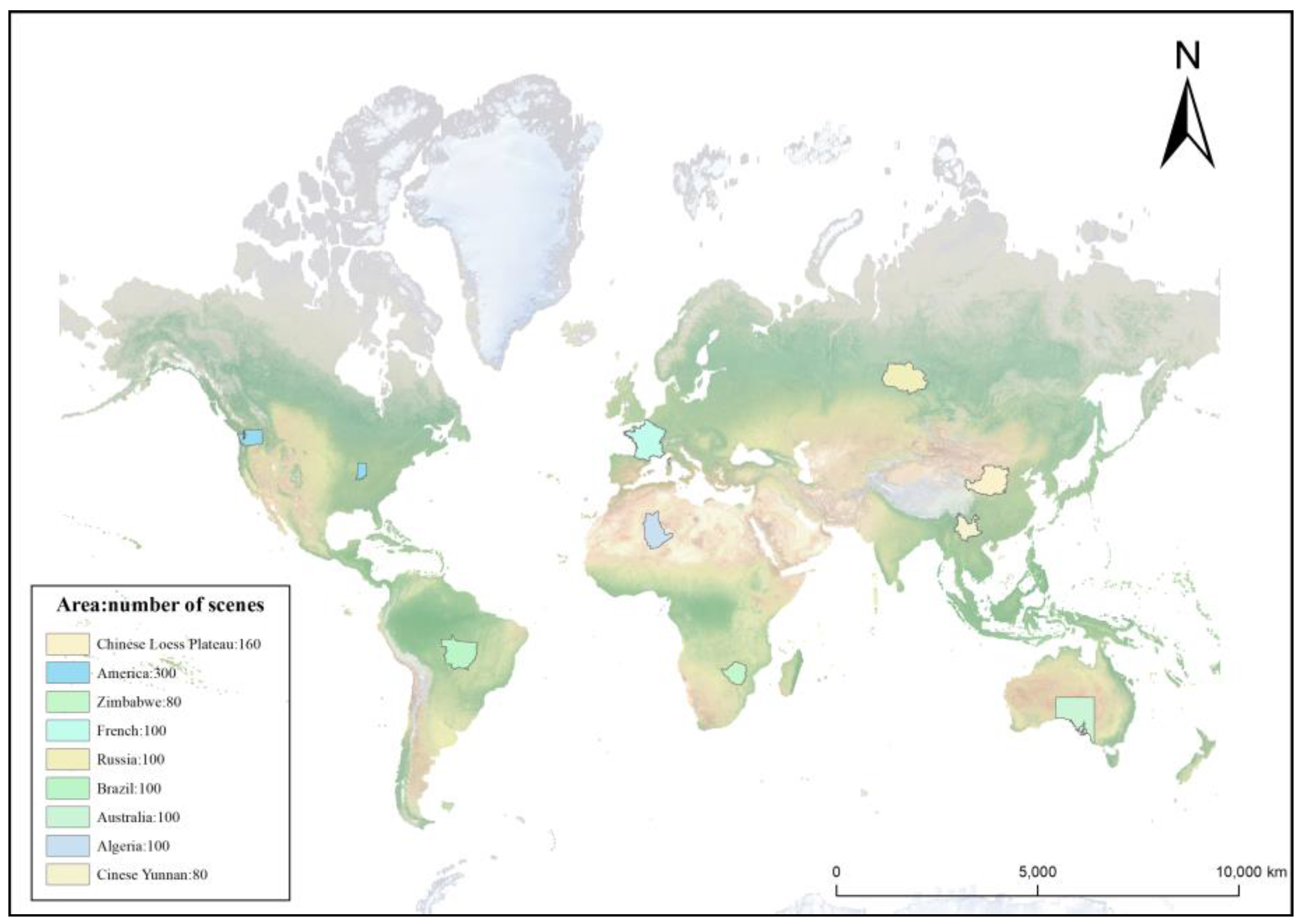
3.1. Customized Dataset Preparation
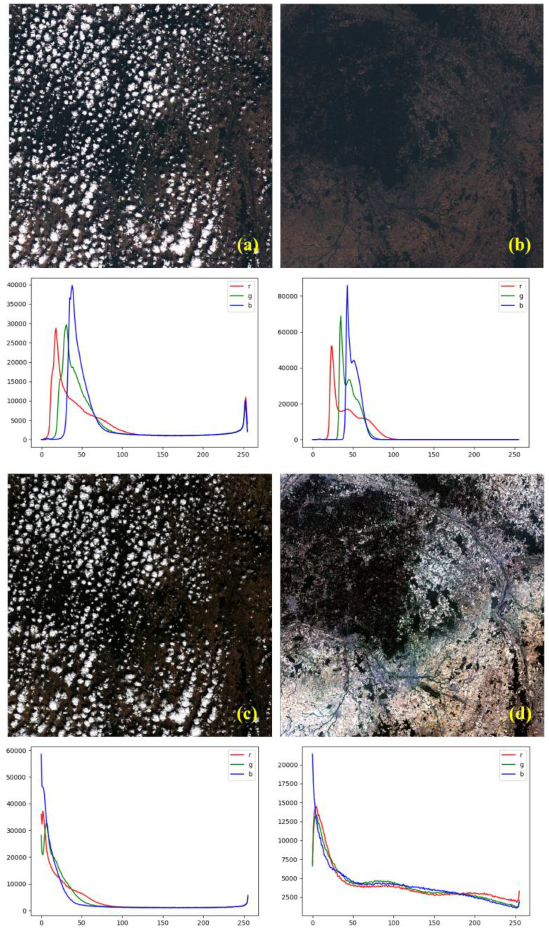
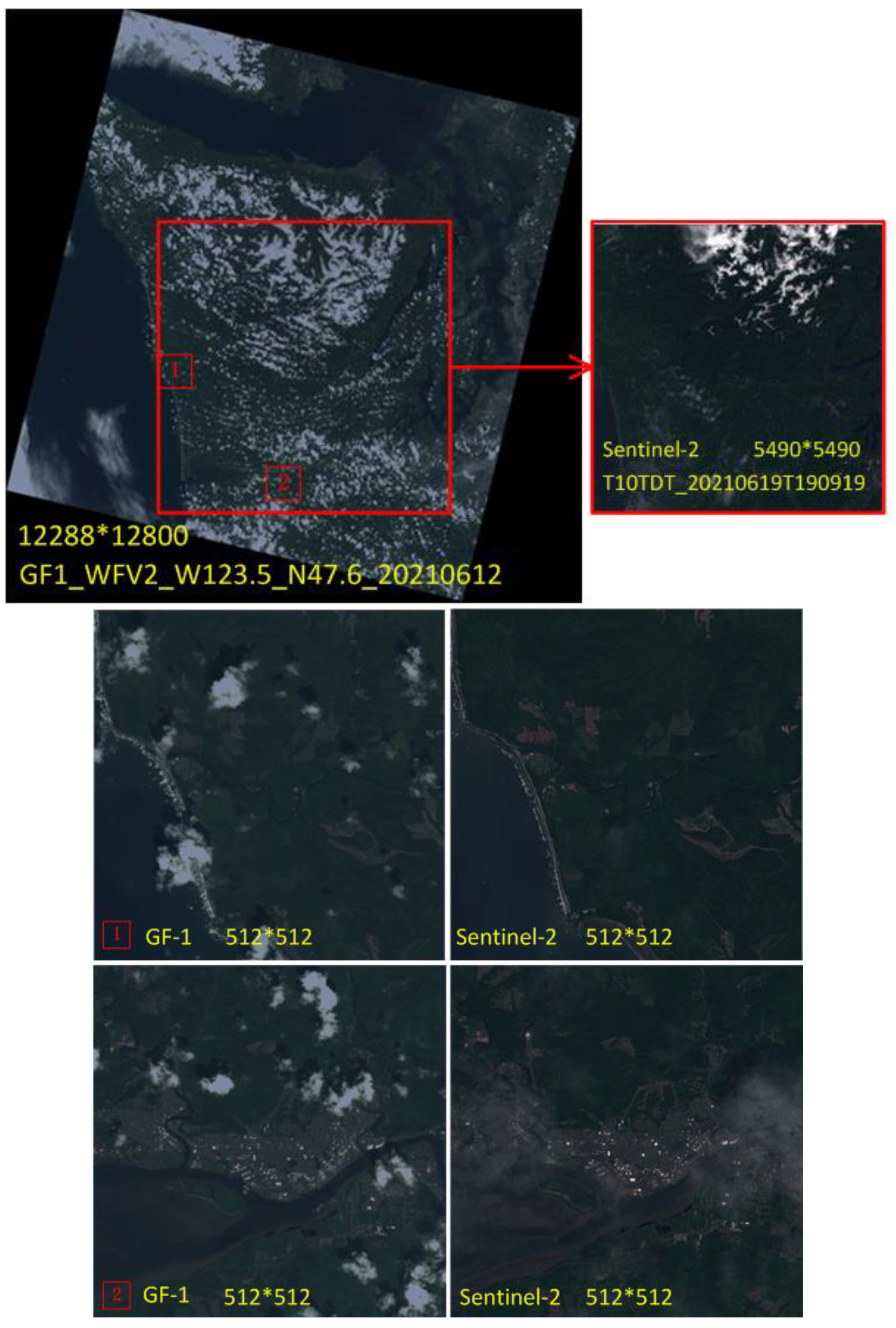
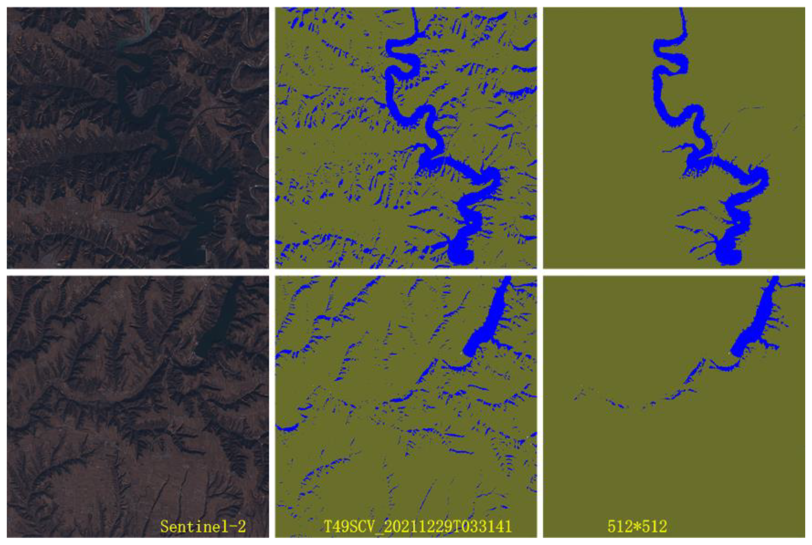
3.1.1. Sample Image
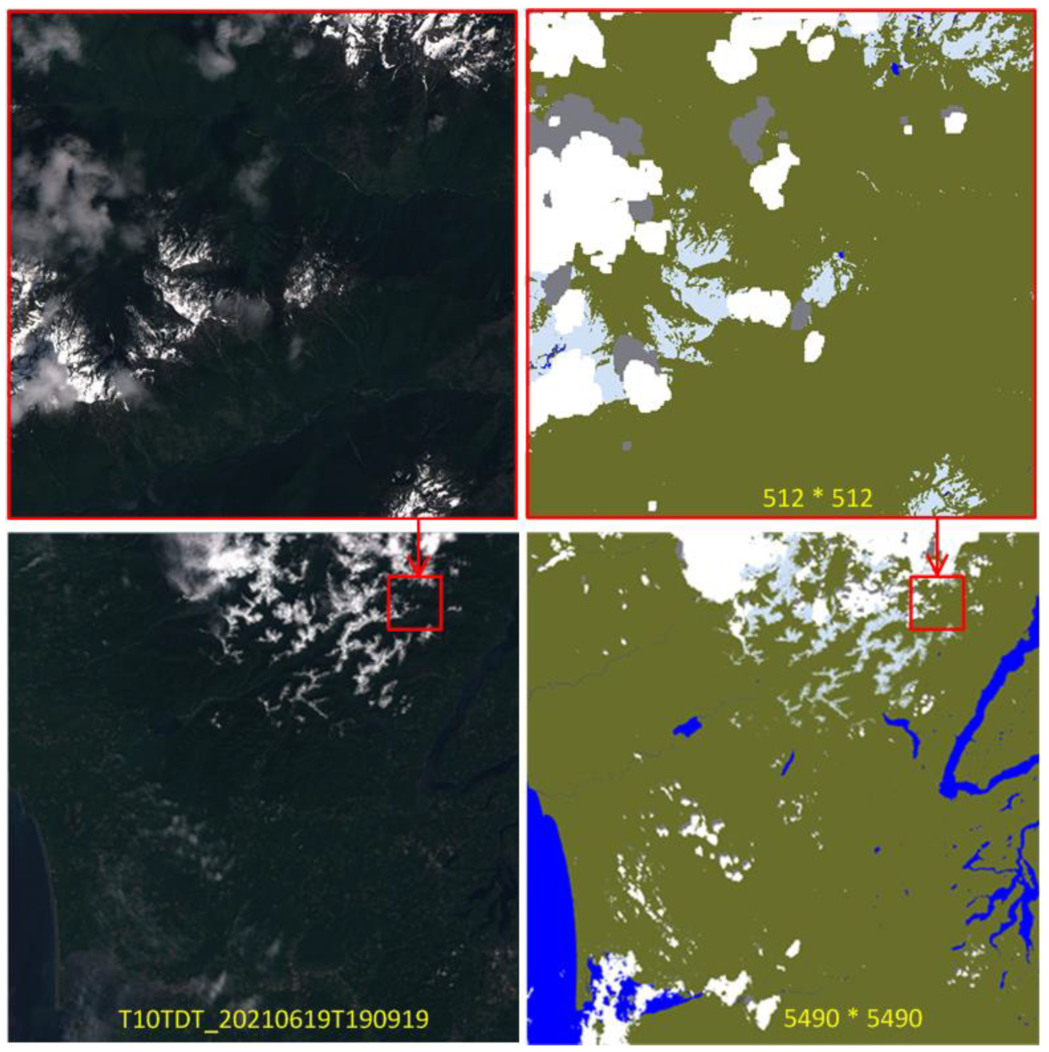
3.1.2. Sample Label
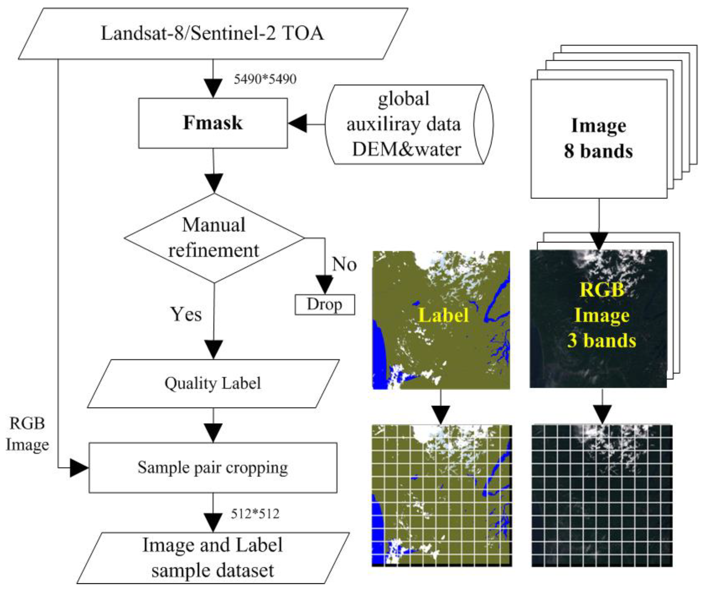
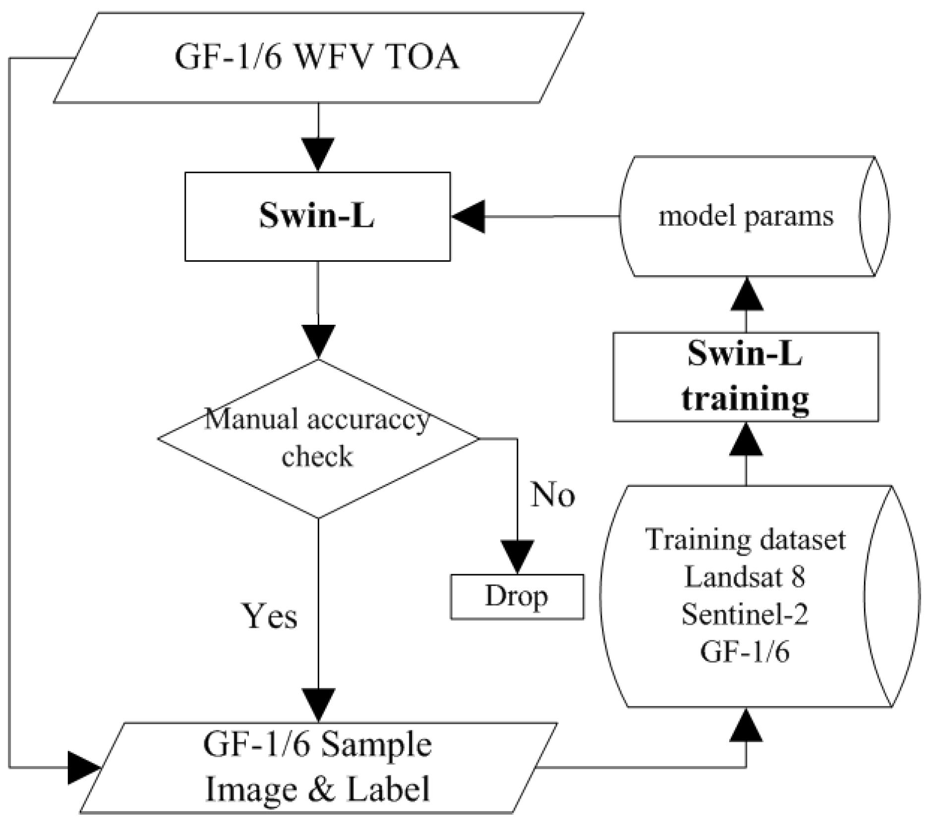
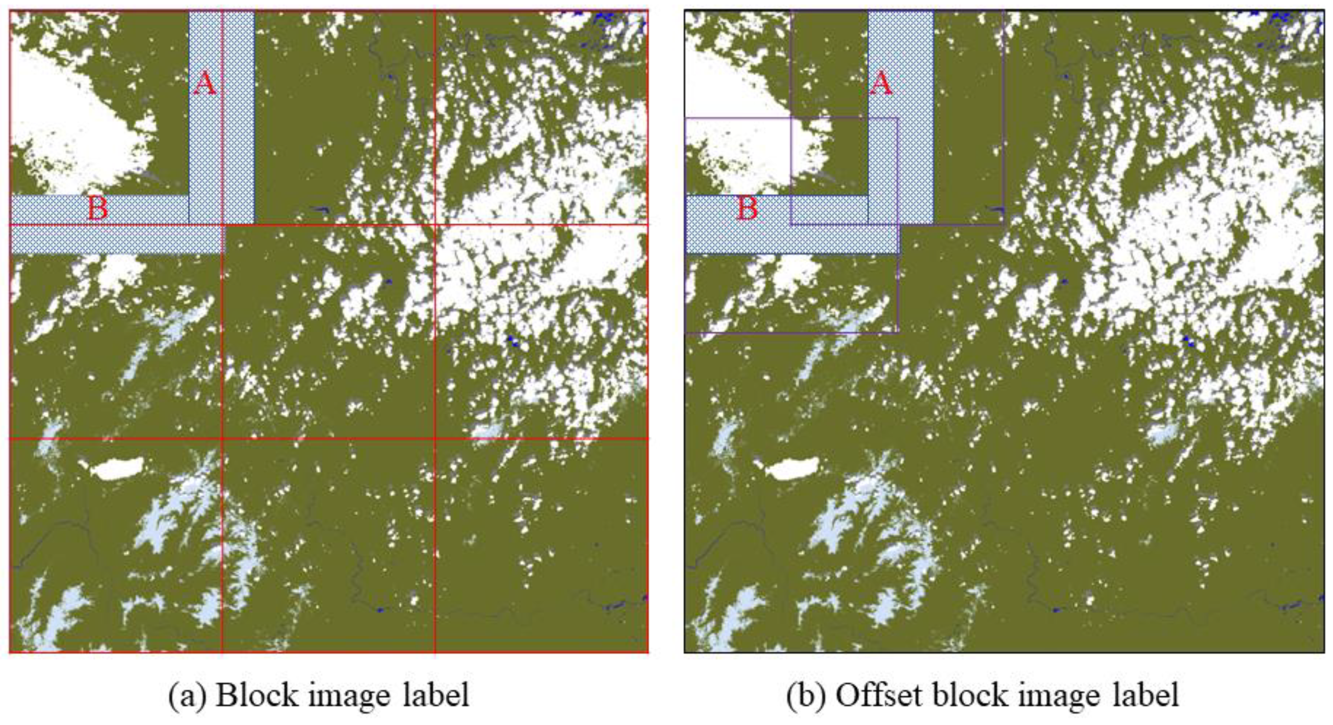
3.1.3. Producing Training Samples
3.2. Algorithm Flow Overview
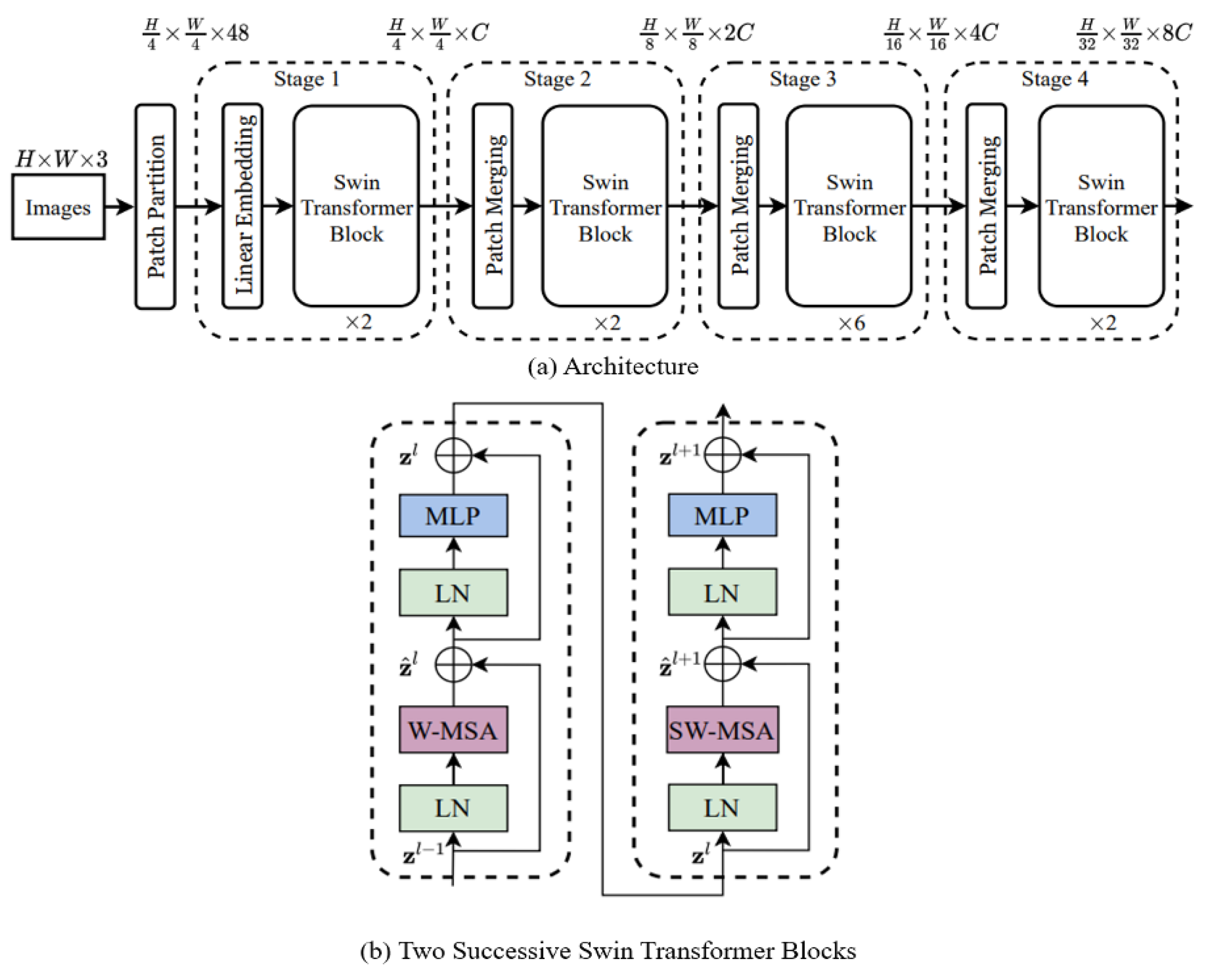
3.2.1. Backbone Network Selection and Training
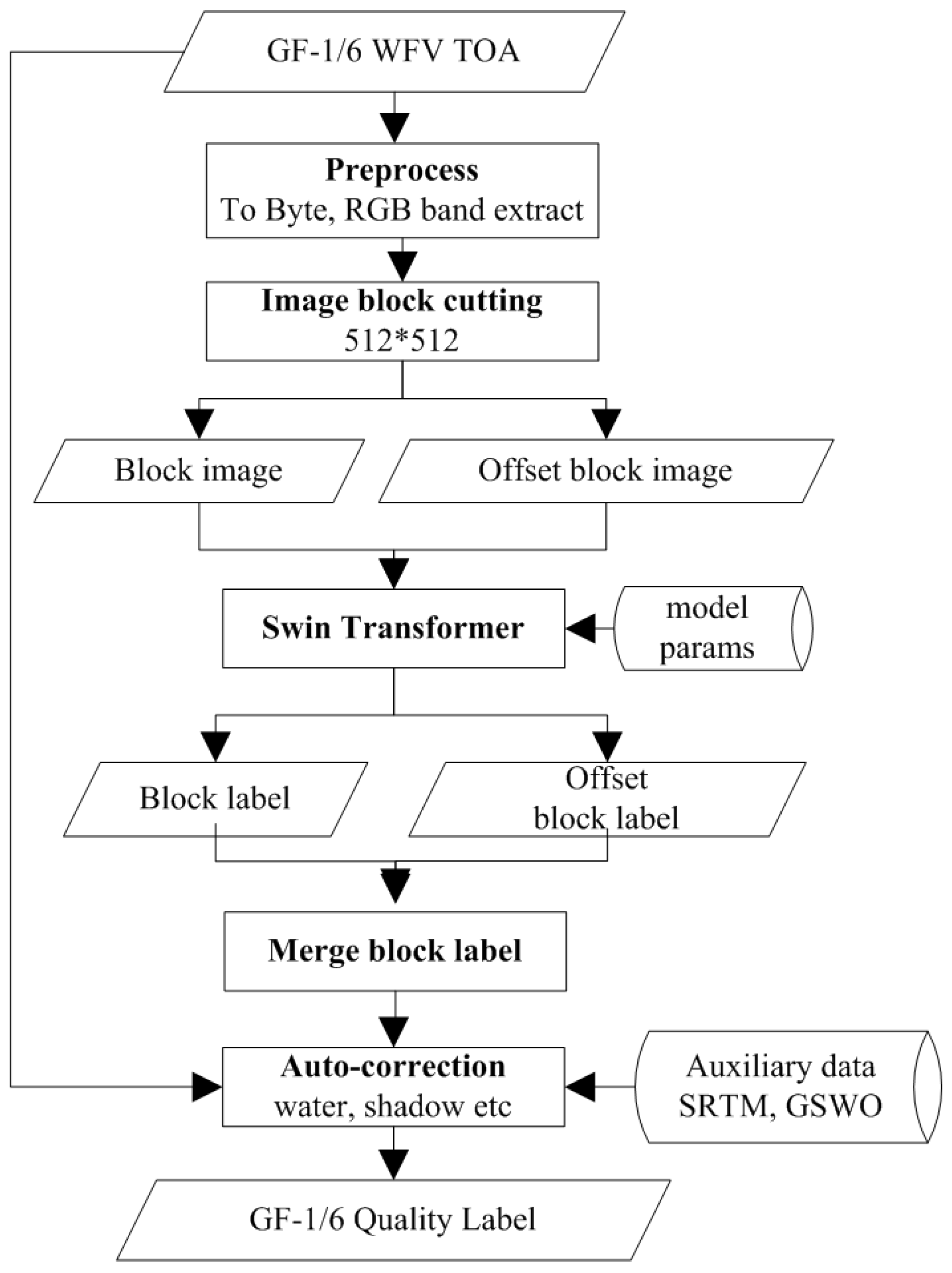
3.2.2. GF-1/6 Quality Tagging Algorithm Flow
3.3. Details in Engineering Application of Quality Tagging
3.3.1. Seam Correction for Chunking Processed Full Image
3.3.2. Automatic Post-Processing Correction
4. Experiment
4.1. Validation Experiment on Customized Dataset
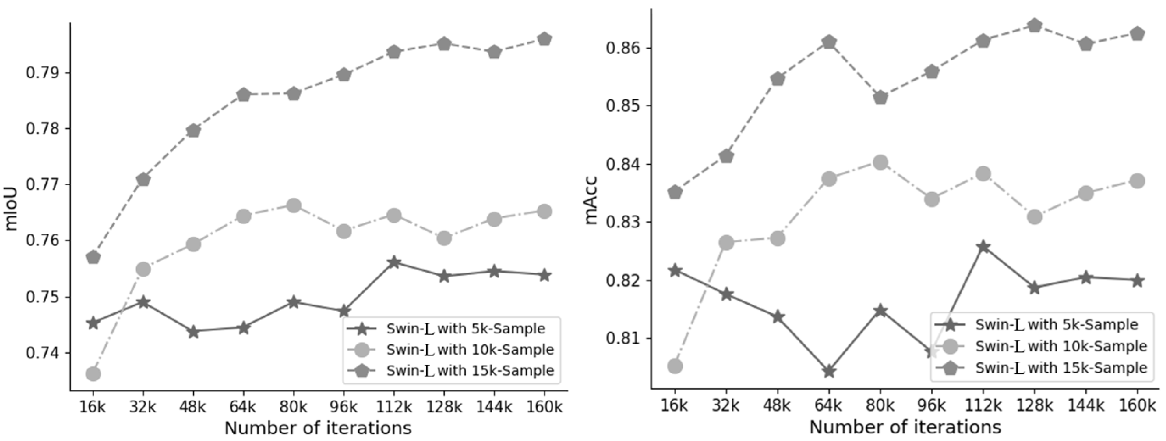
4.1.1. Quantitative Evaluation
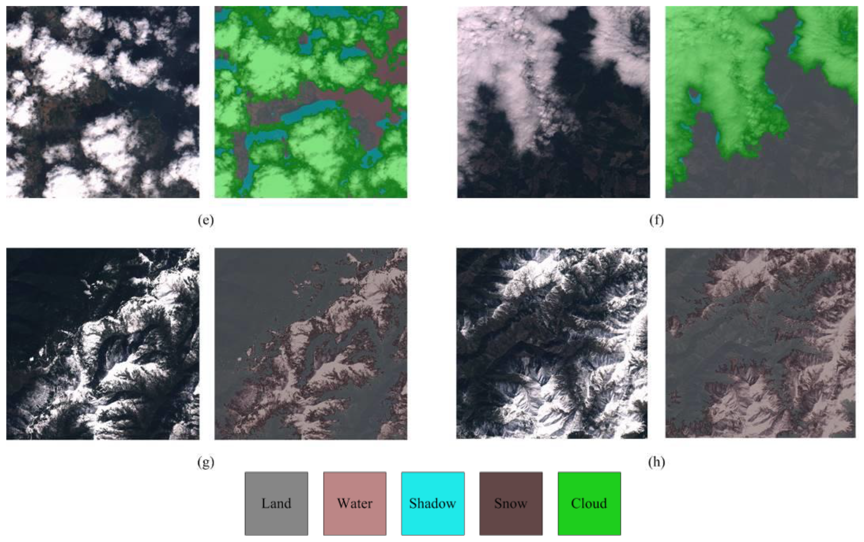
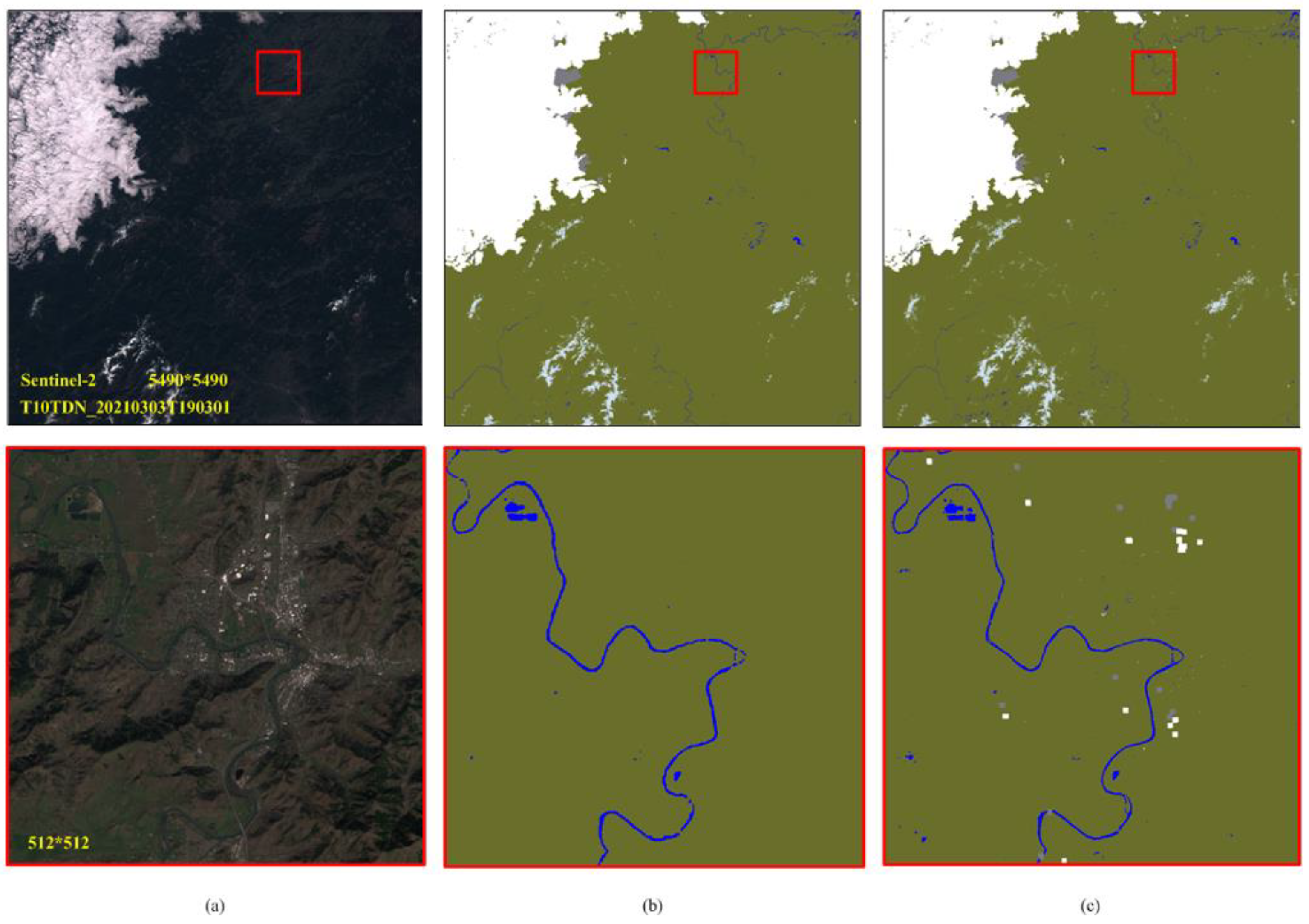
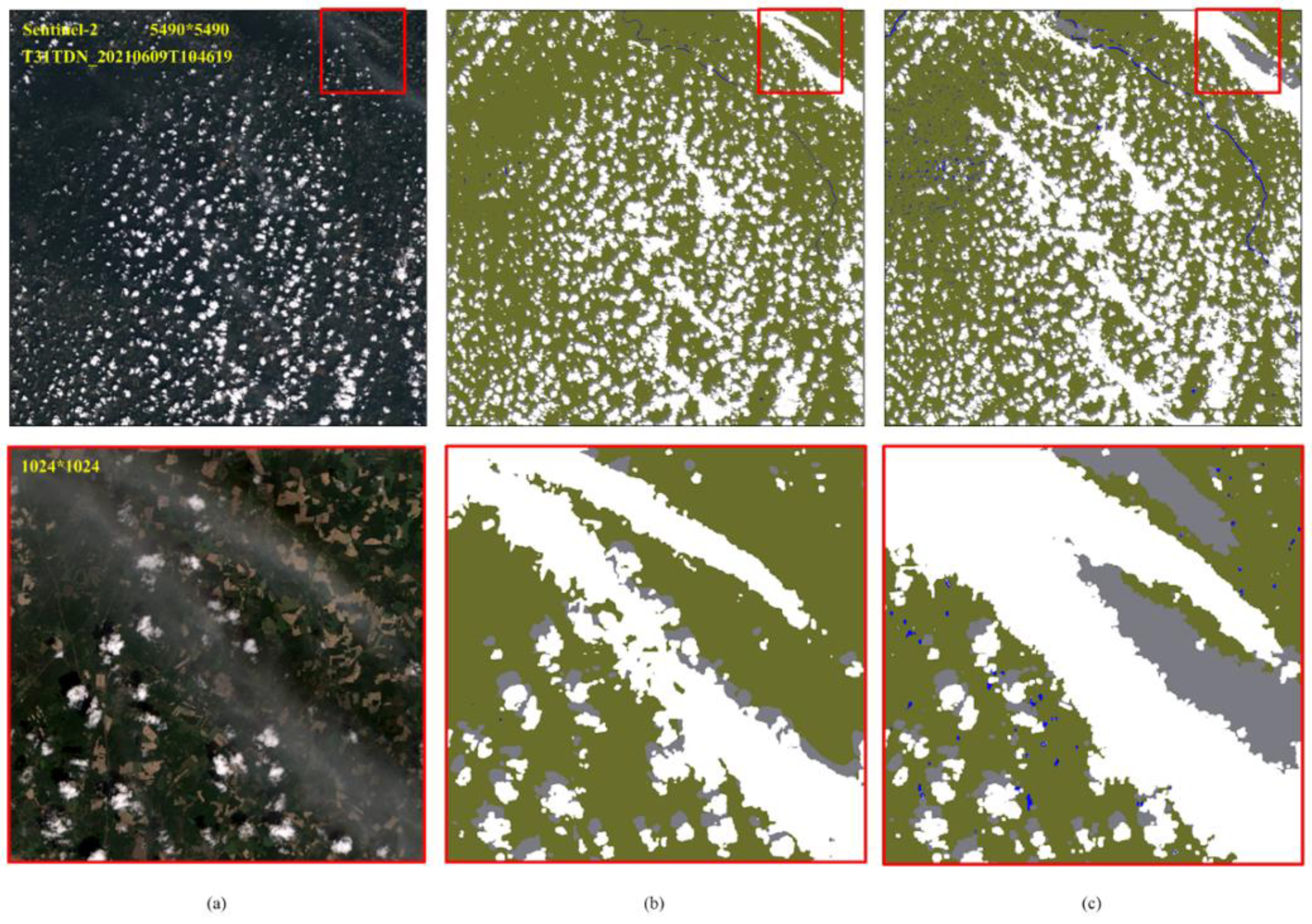
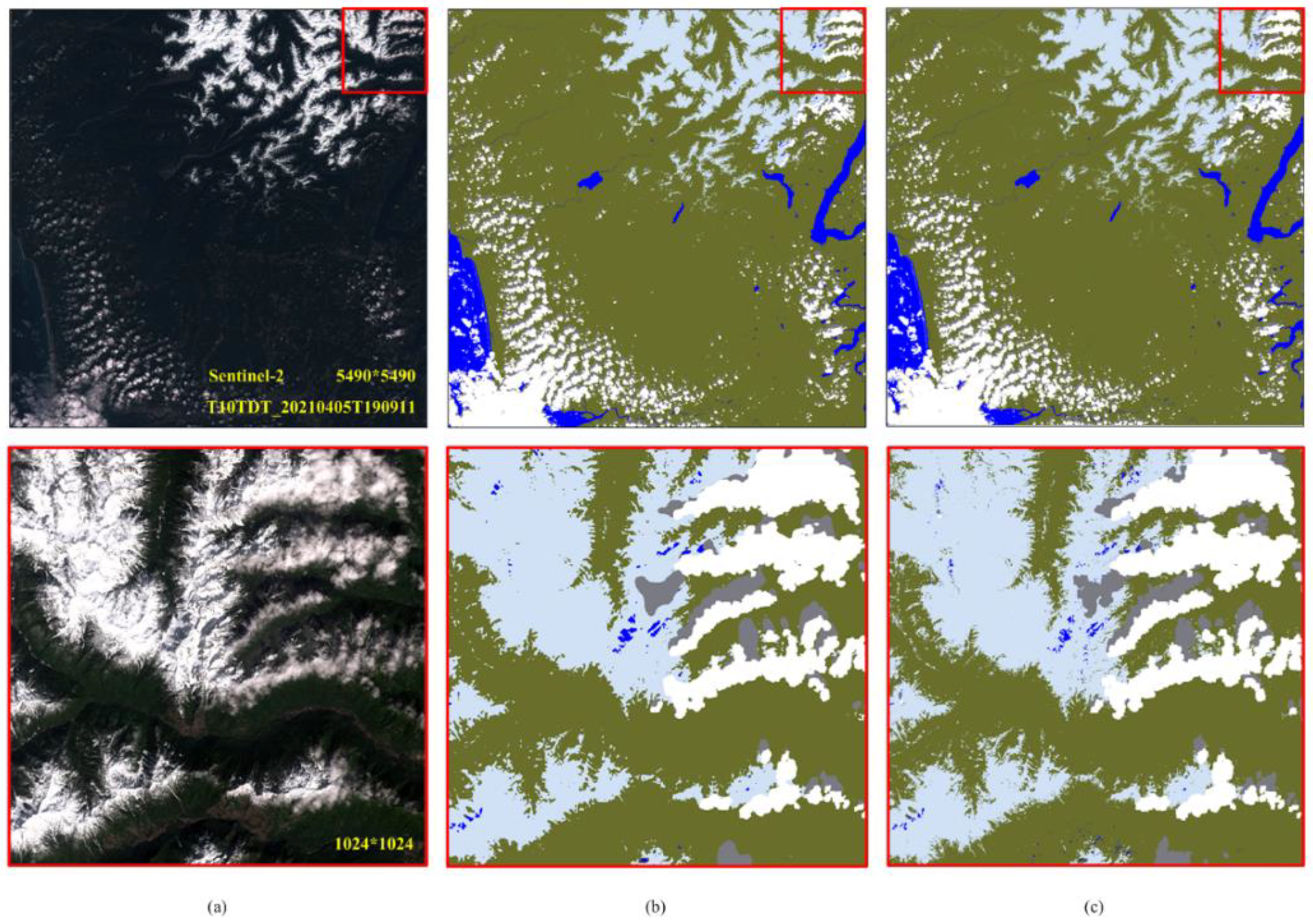
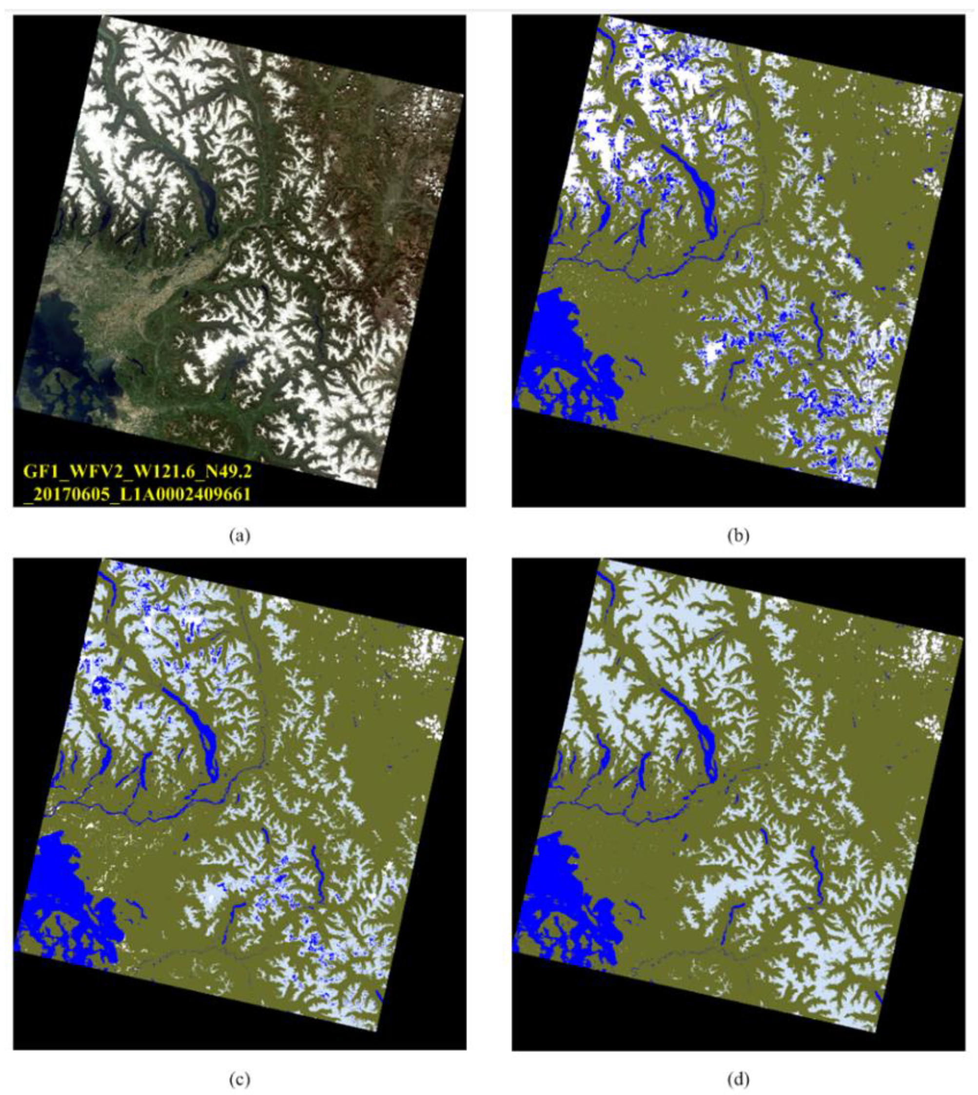
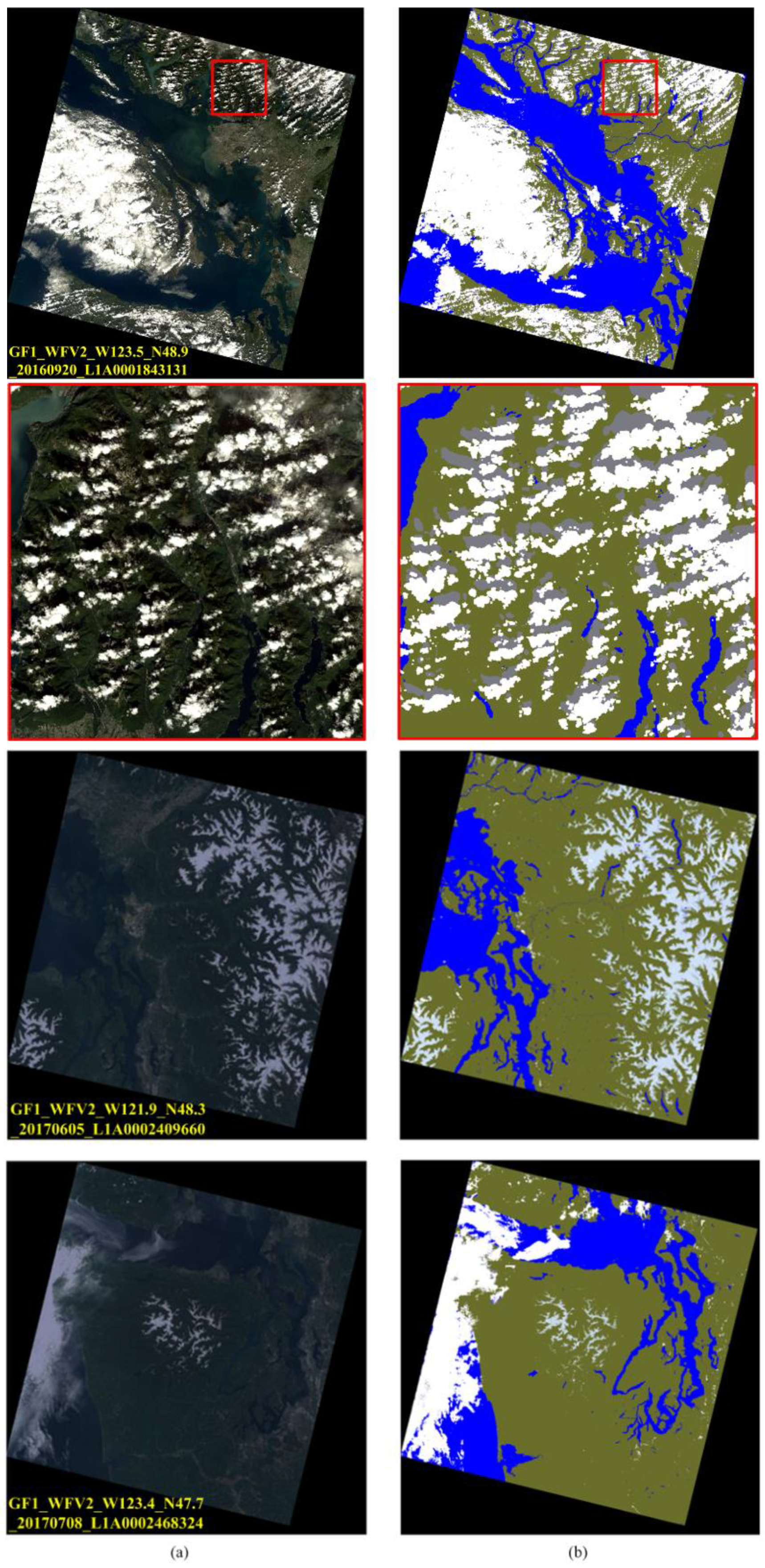
4.1.2. Visual Effect and Comparison with Fmask
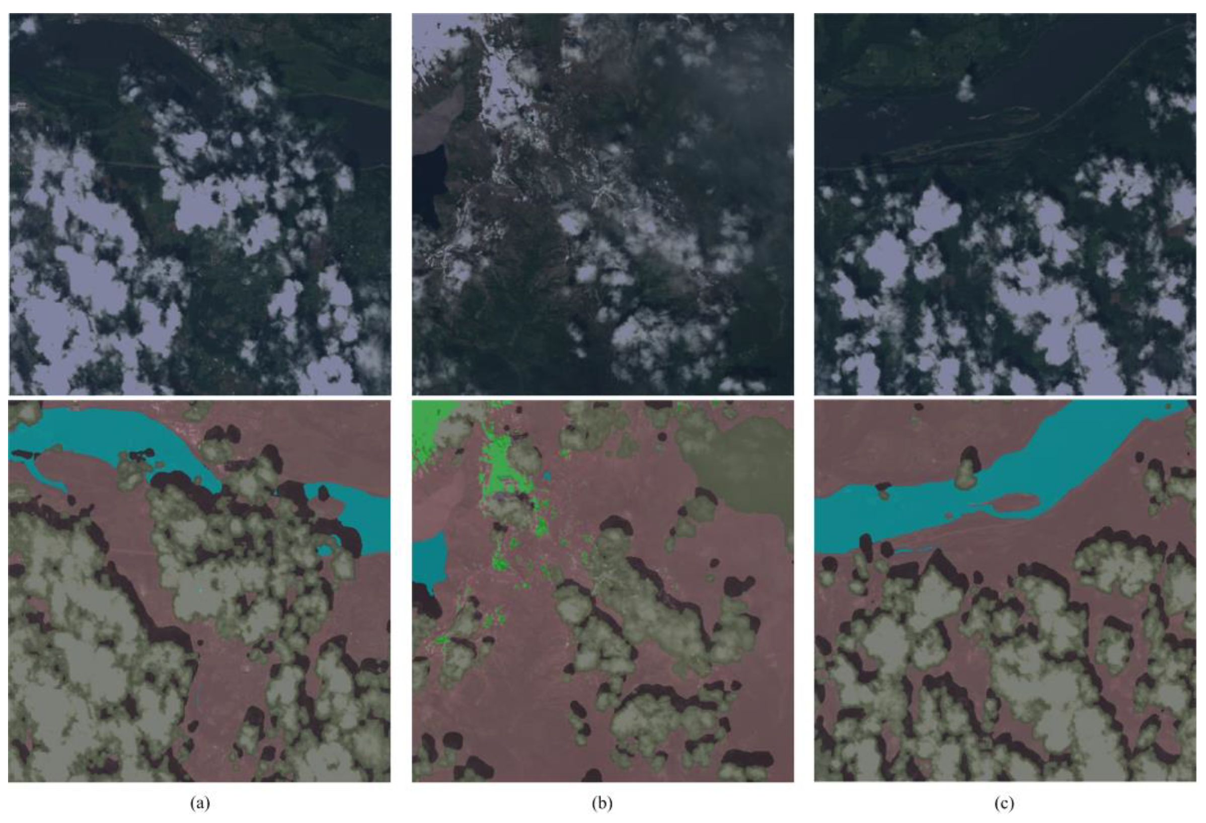
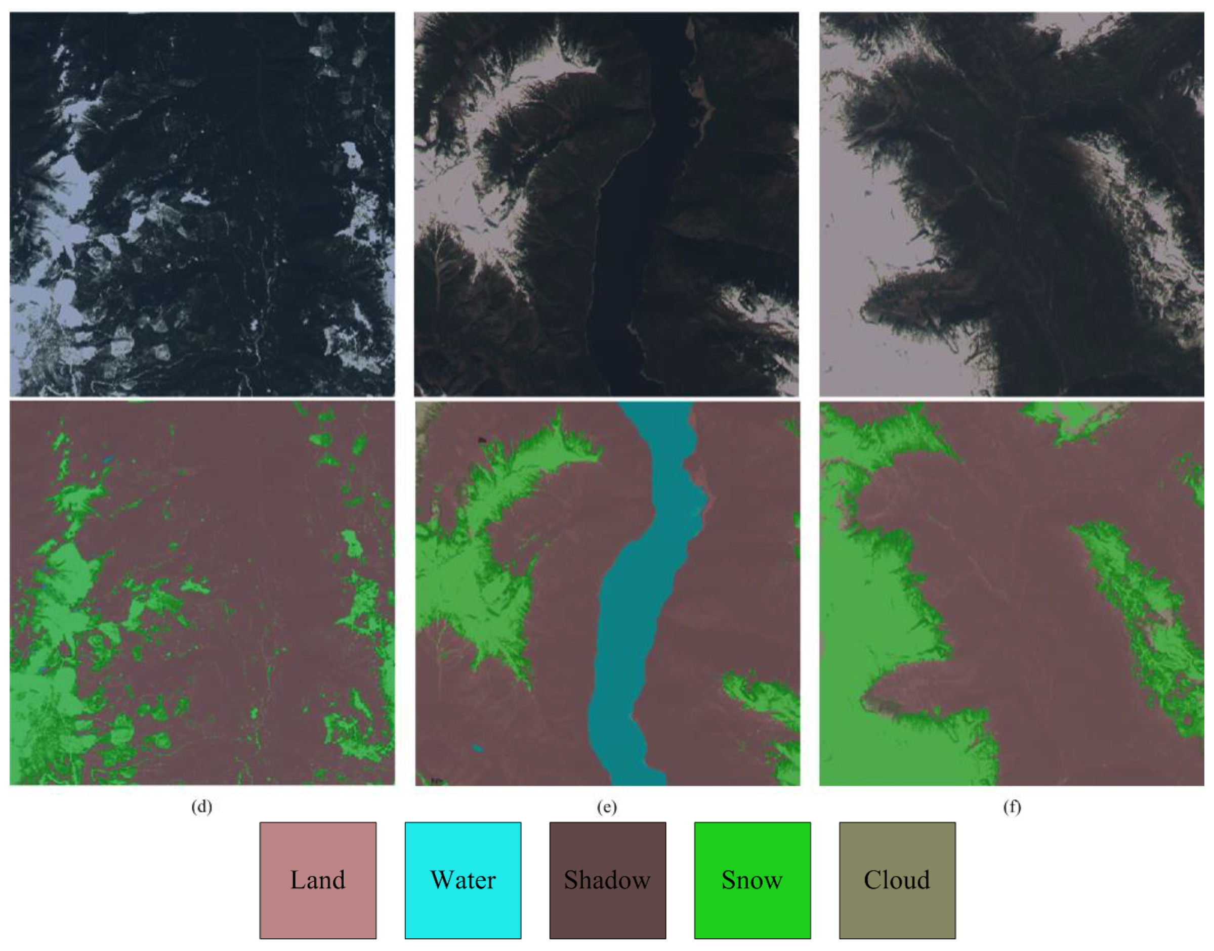
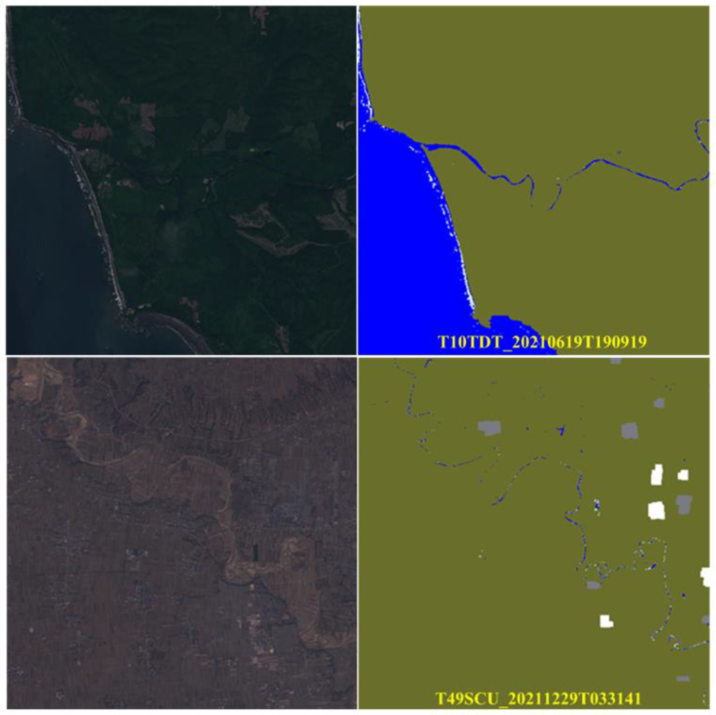
4.2. Producing GF-1/6 Image Quality Tagging Mask
5. Discussion
6. Conclusions
Author Contributions
Funding
Acknowledgments
Conflicts of Interest
Appendix A


References
- Irish, R.R.; Barker, J.L.; Goward, S.N.; Arvidson, T. Characterization of the Landsat-7 ETM+ automated cloud-cover assessment (ACCA) algorithm. Photogramm. Eng. Remote Sens. 2006, 72, 1179–1188. [Google Scholar] [CrossRef]
- Zhu, Z.; Woodcock, C.E. Object-based cloud and cloud shadow detection in Landsat imagery. Remote Sens. Environ. 2012, 118, 83–94. [Google Scholar] [CrossRef]
- Foga, S.; Scaramuzza, P.L.; Guo, S.; Zhu, Z.; Dilley, R.D., Jr.; Beckmann, T.; Schmidt, G.L.; Dwyer, J.L.; Hughes, M.J.; Laue, B. Cloud detection algorithm comparison and validation for operational Landsat data products. Remote Sens. Environ. 2017, 194, 379–390. [Google Scholar] [CrossRef]
- Qiu, S.; Zhu, Z.; He, B. Fmask 4.0: Improved cloud and cloud shadow detection in Landsats 4-8 and Sentinel-2 imagery. Remote Sens. Environ. 2019, 231, 111205. [Google Scholar] [CrossRef]
- Qiu, S.; Lin, Y.; Shang, R.; Zhang, J.; Ma, L.; Zhu, Z. Making Landsat Time Series Consistent: Evaluating and Improving Landsat Analysis Ready Data. Remote Sens. 2019, 11, 51. [Google Scholar] [CrossRef]
- Mahajan, S.; Fataniya, B. Cloud detection methodologies: Variants and development—A review. Complex Intell. Syst. 2020, 6, 251–261. [Google Scholar] [CrossRef]
- Simonyan, K.; Zisserman, A. Very deep convolutional networks for large-scale image recognition. arXiv 2014, arXiv:1409.1556. [Google Scholar]
- He, K.; Zhang, X.; Ren, S.; Sun, J. Deep Residual Learning for Image Recognition. In Proceedings of the IEEE Conference on Computer Vision and Pattern Recognition (CVPR), Las Vegas, NV, USA, 27–30 June 2016. [Google Scholar]
- He, K.; Zhang, X.; Ren, S.; Sun, J. Identity Mappings in Deep Residual Networks. In Computer Vision—ECCV 2016; Leibe, B., Matas, J., Sebe, N., Welling, M., Eds.; Springer International Publishing: Cham, Switzerland, 2016; pp. 630–645. [Google Scholar]
- Huang, G.; Liu, Z.; Van Der Maaten, L.; Weinberger, K.Q. Densely Connected Convolutional Networks. In Proceedings of the 2017 IEEE Conference on Computer Vision and Pattern Recognition (CVPR), Honolulu, HI, USA, 21–26 July 2017; pp. 2261–2269. [Google Scholar]
- Long, J.; Shelhamer, E.; Darrell, T. Fully Convolutional Networks for Semantic Segmentation. IEEE Trans. Pattern Anal. Mach. Intell. 2015, 39, 640–651. [Google Scholar]
- Ronneberger, O.; Fischer, P.; Brox, T. U-Net: Convolutional Networks for Biomedical Image Segmentation; Springer: Cham, Switzerland, 2015; pp. 234–241. [Google Scholar]
- Sun, K.; Zhao, Y.; Jiang, B.; Cheng, T.; Xiao, B.; Liu, D.; Mu, Y.; Wang, X.; Liu, W.; Wang, J. High-Resolution Representations for Labeling Pixels and Regions. arXiv 2019, arXiv:1904.04514. [Google Scholar]
- Chen, L.; Papandreou, G.; Kokkinos, I.; Murphy, K.; Yuille, A.L. Semantic Image Segmentation with Deep Convolutional Nets and Fully Connected CRFs. arXiv 2014, arXiv:1412.7062. [Google Scholar]
- Chen, L.; Papandreou, G.; Kokkinos, I.; Murphy, K.; Yuille, A.L. DeepLab: Semantic Image Segmentation with Deep Convolutional Nets, Atrous Convolution, and Fully Connected CRFs. IEEE Trans. Pattern Anal. Mach. Intell. 2018, 40, 834–848. [Google Scholar] [CrossRef]
- Chen, L.; Papandreou, G.; Schroff, F.; Adam, H. Rethinking Atrous Convolution for Semantic Image Segmentation. arXiv 2017, arXiv:1706.05587. [Google Scholar]
- Chen, L.C.; Zhu, Y.; Papandreou, G.; Schroff, F.; Adam, H. Encoder-Decoder with Atrous Separable Convolution for Semantic Image Segmentation. In Proceedings of the European Conference on Computer Vision (ECCV), Munich, Germany, 8–14 September 2018. [Google Scholar]
- Strudel, R.; Pinel, R.G.; Laptev, I.; Schmid, C. Segmenter: Transformer for Semantic Segmentation. arXiv 2021, arXiv:2105.05633. [Google Scholar]
- Zheng, S.; Lu, J.; Zhao, H.; Zhu, X.; Luo, Z.; Wang, Y.; Fu, Y.; Feng, J.; Xiang, T.; Torr, P.H.S.; et al. Rethinking Semantic Segmentation from a Sequence-to-Sequence Perspective with Transformers. arXiv 2020, arXiv:2012.15840. [Google Scholar]
- Xie, E.; Wang, W.; Yu, Z.; Anandkumar, A.; Alvarez, J.M.; Luo, P. SegFormer: Simple and Efficient Design for Semantic Segmentation with Transformers. arXiv 2021, arXiv:2105.15203. [Google Scholar]
- Petit, O.; Thome, N.; Rambour, C.; Soler, L. U-Net Transformer: Self and Cross Attention for Medical Image Segmentation. arXiv 2021, arXiv:2103.06104. [Google Scholar]
- Hughes, M.; Hayes, D.; Oak Ridge National Lab; Ornl ORTU. Automated Detection of Cloud and Cloud Shadow in Single-Date Landsat Imagery Using Neural Networks and Spatial Post-Processing. Remote Sens. 2014, 6, 4907–4926. [Google Scholar] [CrossRef]
- Chai, D.; Newsam, S.; Zhang, H.K.; Qiu, Y.; Huang, J. Cloud and cloud shadow detection in Landsat imagery based on deep convolutional neural networks. Remote Sens. Environ. 2019, 225, 307–316. [Google Scholar] [CrossRef]
- Jeppesen, J.H.; Jacobsen, R.H.; Inceoglu, F.; Toftegaard, T.S. A cloud detection algorithm for satellite imagery based on deep learning. Remote Sens. Environ. 2019, 229, 247–259. [Google Scholar] [CrossRef]
- Grabowski, B.; Ziaja, M.; Kawulok, M.; Longépé, N.; Saux, B.L.; Nalepa, J. Self-Configuring nnU-Nets Detect Clouds in Satellite Images. arXiv 2022, arXiv:2210.13659. [Google Scholar]
- Jiao, L.; Huo, L.; Hu, C.; Tang, P. Refined UNet: UNet-Based Refinement Network for Cloud and Shadow Precise Segmentation. Remote Sens. 2020, 12, 2001. [Google Scholar] [CrossRef]
- Jiao, L.; Huo, L.; Hu, C.; Tang, P. Refined UNet V2: End-to-End Patch-Wise Network for Noise-Free Cloud and Shadow Segmentation. Remote Sens. 2020, 12, 3530. [Google Scholar]
- Jiao, L.; Huo, L.; Hu, C.; Tang, P. Refined unet v3: Efficient end-to-end patch-wise network for cloud and shadow segmentation with multi-channel spectral features. Neural Networks 2021, 143, 767–782. [Google Scholar]
- Jiao, L.; Huo, L.; Hu, C.; Tang, P.; Zhang, Z. Refined UNet V4, End-to-End Patch-Wise Network for Cloud and Shadow Segmentation with Bilateral Grid. Remote Sens. 2022, 14, 358. [Google Scholar] [CrossRef]
- Liu, Z.; Lin, Y.; Cao, Y.; Hu, H.; Wei, Y.; Zhang, Z.; Lin, S.; Guo, B. Swin transformer: Hierarchical vision transformer using shifted windows. In Proceedings of the IEEE/CVF International Conference on Computer Vision, Montreal, QC, Canada, 10–17 October 2021; pp. 10012–10022. [Google Scholar]
- Li, Z.; Shen, H.; Li, H.; Xia, G.; Gamba, P.; Zhang, L. Multi-feature combined cloud and cloud shadow detection in GaoFen-1 wide field of view imagery. Remote Sens. Environ. 2017, 191, 342–358. [Google Scholar] [CrossRef]
- Wang, M.; Zhang, Z.; Dong, Z.; Jin, S.; Hongbo, S. Stream-computing Based High Accuracy On-board Real-time Cloud Detection for High Resolution Optical Satellite Imagery. Acta Geodaet. Cartogr. Sin. 2018, 47, 76–769. [Google Scholar] [CrossRef]
- Li, T.T.; Tang, X.M.; Gao, X.M. Research on separation of snow and cloud in ZY-3 image cloud recognition. Bull. Survey. Mapp. 2016, 0, 46–49+68. [Google Scholar]
- Guo, Y.; Xiaoqun, C.; Bainian, L.; Mei, G. Cloud Detection for Satellite Imagery Using Attention-Based U-Net Convolutional Neural Network. Symmetry 2020, 12, 1056. [Google Scholar] [CrossRef]
- Vaswani, A.; Shazeer, N.; Parmar, N.; Uszkoreit, J.; Jones, L.; Gomez, A.N.; Kaiser, Ł.; Polosukhin, I. Attention is all you need. arXiv 2017, arXiv:1706.03762. [Google Scholar]
- Dosovitskiy, A.; Beyer, L.; Kolesnikov, A.; Weissenborn, D.; Zhai, X.; Unterthiner, T.; Dehghani, M.; Minderer, M.; Heigold, G.; Gelly, S.; et al. An Image is Worth 16x16 Words: Transformers for Image Recognition at Scale; International Conference on Learning Representations. arXiv 2021, arXiv:2010.11929. [Google Scholar]
- Zhu, Z.; Woodcock, C.E. Improvement and Expansion of the Fmask Algorithm: Cloud, Cloud Shadow, and Snow Detection for Landsats 4-7, 8, and Sentinel 2 images. Remote Sens. Environ. 2014, 159, 269–277. [Google Scholar] [CrossRef]
- Qiu, S.; He, B.; Zhu, Z.; Liao, Z.; Quan, X. Improving Fmask cloud and cloud shadow detection in mountainous area for Landsats 4–8 images. Remote Sens. Environ. 2017, 199, 107–119. [Google Scholar] [CrossRef]
- Xiao, T.; Liu, Y.; Zhou, B.; Jiang, Y.; Sun, J. Unified perceptual parsing for scene understanding; In Proceedings of the European Conference on Computer Vision (ECCV). arXiv 2018, arXiv:1807.1022; pages 418–434, 418–434. [Google Scholar]
- MMSegmentation Contributors. MMSegmentation: Openmmlab Semantic Segmentation Toolbox and Benchmark. 2020. Available online: https://github.com/open-mmlab/mmsegmentation (accessed on 10 November 2022).


| Satellite | Landsat-8 | Sentinel-2A | Sentinel-2B | GF-1 | GF-6 |
|---|---|---|---|---|---|
| Coastal Blue | 0.433–0.453 | 0.432–0.453 | 0.432–0.453 | --- | 0.40–0.45 |
| Blue | 0.450–0.515 | 0.459–0.525 | 0.459–0.525 | 0.45–0.52 | 0.45–0.52 |
| Green | 0.525–0.600 | 0.542–0.578 | 0.541–0.577 | 0.52–0.59 | 0.52–0.59 |
| Yellow | --- | --- | --- | --- | 0.59–0.63 |
| Red | 0.630–0.680 | 0.649–0.680 | 0.650–0.681 | 0.63–0.69 | 0.63–0.69 |
| Red Edge 1 | --- | 0.697–0.712 | 0.696–0.712 | --- | 0.69–0.73 0.73–0.77 |
| Red Edge 2 | 0.733–0.748 | 0.732–0.747 | |||
| Red Edge 3 | 0.773–0.793 | 0.770–0.790 | |||
| NIR Narrow NIR | 0.845–0.885 | 0.780–0.886 0.854–0.875 | 0.780–0.886 0.853–0.875 | 0.77–0.89 | 0.77–0.89 |
| Water vapor | --- | 0.935–0.955 | 0.933–0.954 | --- | --- |
| Cirrus | 1.360–1.390 | 1.358–1.389 | 1.362–1.392 | --- | --- |
| SWIR 1 | 1.560–1.660 | 1.568–1.659 | 1.563–1.657 | --- | --- |
| SWIR 2 | 2.100–2.300 | 2.115–2.290 | 2.093–2.278 | --- | --- |
| TIRS 1 | 10.60–11.19 | --- | --- | --- | --- |
| TIRS 2 | 11.50–12.51 | --- | --- | --- | --- |
| UInt16 | Byte | Memo |
|---|---|---|
| 0 | 0 | Fill value |
| 1–6000 | 1–250 | Step length 24 |
| 6001–10,000 | 251–254 | Step length 1000 |
| >10,000 | 255 | Saturation value |
| Class | Land | Water | Cloud Shadow | Snow | Cloud | Fill Value |
|---|---|---|---|---|---|---|
| Label | 1 | 2 | 3 | 4 | 5 | 0 |
| RGB |  |  |  |  |  |  |
| Model | mIoU (%) | mAcc (%) | Land (1) | Water (2) | Shadow (3) | Snow (4) | Cloud (5) | |||||
|---|---|---|---|---|---|---|---|---|---|---|---|---|
| IoU (%) | Acc (%) | IoU (%) | Acc (%) | IoU (%) | Acc (%) | IoU (%) | Acc (%) | IoU (%) | Acc (%) | |||
| HRNet | 74.78 | 81.34 | 90.01 | 97.19 | 86.54 | 90.15 | 54.77 | 67.58 | 53.49 | 59.79 | 89.09 | 91.98 |
| DeepLabv3 | 73.49 | 81.13 | 89.68 | 96.62 | 86.88 | 90.74 | 51.74 | 62.51 | 51.58 | 63.53 | 87.60 | 91.93 |
| Swin-S | 70.50 | 77.63 | 86.71 | 96.85 | 72.13 | 74.11 | 51.19 | 64.79 | 54.33 | 60.68 | 88.12 | 91.72 |
| Swin-B | 75.27 | 82.46 | 90.08 | 97.28 | 87.37 | 90.70 | 52.90 | 64.62 | 57.25 | 67.66 | 88.76 | 92.02 |
| Swin-L | 76.53 | 83.72 | 90.86 | 97.39 | 89.22 | 93.61 | 54.30 | 64.82 | 58.82 | 70.23 | 89.47 | 92.54 |
Disclaimer/Publisher’s Note: The statements, opinions and data contained in all publications are solely those of the individual author(s) and contributor(s) and not of MDPI and/or the editor(s). MDPI and/or the editor(s) disclaim responsibility for any injury to people or property resulting from any ideas, methods, instructions or products referred to in the content. |
© 2023 by the authors. Licensee MDPI, Basel, Switzerland. This article is an open access article distributed under the terms and conditions of the Creative Commons Attribution (CC BY) license (https://creativecommons.org/licenses/by/4.0/).
Share and Cite
Fan, X.; Chang, H.; Huo, L.; Hu, C. GF-1/6 Satellite Pixel-by-Pixel Quality Tagging Algorithm. Remote Sens. 2023, 15, 1955. https://doi.org/10.3390/rs15071955
Fan X, Chang H, Huo L, Hu C. GF-1/6 Satellite Pixel-by-Pixel Quality Tagging Algorithm. Remote Sensing. 2023; 15(7):1955. https://doi.org/10.3390/rs15071955
Chicago/Turabian StyleFan, Xin, Hao Chang, Lianzhi Huo, and Changmiao Hu. 2023. "GF-1/6 Satellite Pixel-by-Pixel Quality Tagging Algorithm" Remote Sensing 15, no. 7: 1955. https://doi.org/10.3390/rs15071955
APA StyleFan, X., Chang, H., Huo, L., & Hu, C. (2023). GF-1/6 Satellite Pixel-by-Pixel Quality Tagging Algorithm. Remote Sensing, 15(7), 1955. https://doi.org/10.3390/rs15071955