Abstract
The three-dimensional (3D) geometry reconstruction method utilizing ISAR image sequence energy accumulation (ISEA) shows great performance on triaxial stabilized space targets but fails when there is unknown motion from the target itself. The orthogonal factorization method (OFM) can solve this problem well under certain assumptions. However, due to the sparsity and anisotropy of ISAR images, the extraction and association of feature points become very complicated, resulting in the reconstructed geometry usually being a relatively sparse point cloud. Therefore, combining the advantages of the above methods, an extended factorization framework (EFF) is proposed. First, the instance segmentation method based on deep learning is used for the extraction and association of a number of key points on multi-view ISAR images. Then, the projection vectors between the 3-D geometry of the space target and the multi-view ISAR images are obtained, using the improved factorization method. Finally, the 3D geometry reconstruction problem is transformed into an unconstrained optimization problem and solved via the quantum-behaved particle swarm optimization (QPSO) method. The proposed framework uses discretely observed multi-view range–Doppler ISAR images as an input, which can make full use of the long-term data of space targets from multiple perspectives and which is non-sensitive to movement. Therefore, the proposed framework shows high feasibility in practical applications. Experiments on simulated and measured data show the effectiveness and robustness of the proposed framework.
1. Introduction
Inverse synthetic aperture radar (ISAR) is one of the most effective methods in space situational awareness due to its ability to acquire high-resolution images of long-range targets throughout the day and in all weather conditions [1,2,3,4,5,6]. With the development of radar technology, the resolution of ISAR images has been greatly improved in the last few decades, but the essence of ISAR imaging has not changed. Specifically, ISAR images are two-dimensional (2D) projections of the electromagnetic scattering characteristics of the three-dimensional (3D) surface of a target on the radar’s imaging planes. Therefore, they struggle to accurately depict the 3D structure of a target directly and effectively. In addition, humankind’s enthusiasm for space exploration has been unprecedentedly high in recent years, resulting in more and more spacecrafts being launched into space. The types of spacecrafts are also becoming increasingly diversified, while their structures are becoming increasingly complex, leading to the limitations in the accurate classification and recognition of space targets using 2D ISAR images gradually becoming more prominent. However, the 3D structure of space targets can provide information about their geometry in a more elegant way, which makes research on 3D imaging technology in ISAR a hot topic in the field of space situational awareness.
According to the number of receiving channels in a radar system, ISAR 3D imaging methods can be divided into two categories, i.e., methods based on multiple receiving channels [7,8,9,10,11,12,13,14,15,16] and methods based on one receiving channel [17,18,19]. With four receiving channels distributed along the pitch and azimuth directions, monopulse radar can obtain angle measurements for different scatterers relative to the radar. Combined with a high resolution in the range direction, different scatterers can be distinguished on targets, which means that monopulse radar can determine the 3D geometry of targets [7,8,9]. This process was the earliest instance of exploring ISAR 3D imaging, but the accuracy highly depended on the accuracy of the angle measurements. Therefore, the performance of 3D imaging for small or far away targets deteriorated sharply.
Subsequently, researchers started to focus on 3D imaging methods that use interferometric ISAR (InISAR). These methods have shown great potential. InISAR can carry out 3D imaging by providing height information contained in the phase of corresponding scatterers after registering the multi-view ISAR images obtained by different radars [10,11,12,13]. The 3D imaging mechanism of InISAR determines the level of complexity of its hardware system. Specifically, the distribution of radars and the accuracy of time–frequency synchronization must be guaranteed in the InISAR system in order to ensure coherence between the images obtained by each radar. Accordingly, applications of InISAR systems are currently limited to laboratory environments, although InISAR 3D imaging theory has been greatly developed. On the other hand, in 3D imaging technology based on a radar network with known or solvable projection vectors, the projection process of ISAR imaging can be modeled as projection equations. Then, the 3D geometry of the target can be obtained by solving the projection equations. This process makes full use of the multi-view information of radar networks, so it only needs a short observation time to recover the 3D geometry of a target [14,15,16].
The second category of 3D imaging methods is based on a single receiving channel. In this category, the factorization method is most widely used. By providing the projected positions of four non-coplanar points in three different views, the 3D relative coordinates of those points can be obtained by decomposing the projection position matrix of the four points [20]. The scatterer extraction of different ISAR images is the prerequisite. Many classical and effective feature point extraction algorithms have been proposed [21,22,23,24,25]. However, compared with optical images, ISAR images are sparser and have less textural information, resulting in difficulty when extracting extra scatterers from an ISAR image sequence. As a result, the reconstructed geometry looks rather sparse when the factorization method is directly applied to ISAR images. In fact, both the radar network-based 3D imaging technologies and the single-channel ISAR-based 3D imaging technologies make use of the multi-view ISAR images of the target. The only difference lies in the fact that the multi-view information utilized in the single-channel ISAR-based 3D imaging technologies comes from the relative motion between the target and the radar during long-term observation. Therefore, there is great benefit when the projection positions of the scatterers on multi-view ISAR images are able to form continuous trajectories. Hence, scatterers’ trajectories can be used to make full use of the target motion models [26,27,28,29].
In [26], the observed target was modeled as a slowly rotating target, on the basis of which the authors proved that the projected trajectories of the scatterers on the imaging plane were ellipses. Thereafter, the Markov Chain Monte Carlo Data Association (MMCDA) method was used to associate the scatterer trajectories. A new trajectory association method, based on the multiple hypothesis tracking (MHT) algorithm under the same circumstances, was proposed in [27]; that method improved the tracing performance when the observed trajectories were very incomplete. However, the multi-view ISAR images used in the above algorithms must be properly registered. Unfortunately, the cross-range scaling factors in ISAR images depend highly on the estimation precision of the effective rotation motion of the target. The estimated errors in the cross-range scaling factors severely degrade the performance of the algorithms when the motion is unknown.
Although more and more feature point extraction and association algorithms have been proposed, the application scenarios are usually limited to a specified target motion model. The extraction and association of scatterers are still the biggest obstacles when the factorization method is applied in ISAR 3D imaging. In this regard, a new 3D imaging method based on ISAR image sequence energy accumulation (ISEA) was proposed in [30]. The algorithm uses the fact that the projected positions of real scatterers on targets show higher energy in most images. By constructing the projection vectors from the 3D geometry of the triaxial stabilized space target to the 2D ISAR image sequence via an instantaneous radar line of sight (LOS), the 3D geometry can be reconstructed using the particle swarm optimization (PSO) algorithm. This method does not need to map the reconstructed scatterers to the extracted ones in ISAR images one-to-one, so there is no need to extract and associate scatterers, thus showing better robustness. On the other hand, the construction of the projection vectors completely depends on the LOS. They cannot be obtained accurately when there is additional rotation of the targets, which invalidates the algorithm. To solve this problem, the ISEA method was improved in [31] by re-modeling the motion of a space target. This improved method indicated that the 3D imaging of a target can still be realized via iterative optimization between the motion parameters and the coordinates of the 3D scatterers when the motion of the space target satisfies the fixed axis slow-rotation model.
However, the observed targets are generally non-cooperative, which means that it is difficult to describe their motion state with a precise motion model. Therefore, this paper proposes an extended factorization framework (EFF) based on the structure from motion (SFM) theory. First, by taking advantage of the characteristic that all scatterers share the same projection vectors at the same time, the positions of several key points are extracted via the feature point extraction method, based on deep learning. Then, the 3D coordinates and the instantaneous projection vectors of these key points can be calculated via the improved factorization method, and the 3D reconstruction problem can be modeled as an unconstrained optimization problem. Finally, the dense point cloud of the target can be obtained by solving the unconstrained optimization problem via the quantum-behaved particle swarm optimization (QPSO) algorithm. The proposed EFF can be a general framework for ISAR 3D imaging without limiting the motion of targets, showing great performance in real scenarios.
The remainder of this paper is arranged as follows: Section 2 introduces the geometry of multi-view ISAR imaging and analyzes the limitations of the 3D reconstruction method based on specific motion modeling. Then, the EFF and its key steps are described in detail, followed by an analysis and definition of some indicators to measure the performance of the algorithm. In Section 3, the effectiveness and robustness of the proposed method are verified via experiments with simulated data and measured data. Section 4 discusses the results of the experiments. Finally, conclusions are drawn in Section 5.
2. Materials and Methods
2.1. ISAR Observation Geometry
The ISAR imaging geometry of the space target is shown in Figure 1a. The geometry of a satellite , i.e., the matrix of 3D coordinates of different scatterers, is defined in the orbital coordinate system (OCS) [32], which can be obtained by rotating the geometry in the body coordinate system (BCS) of the satellite via the attitude transformation matrix . Without any loss of generality, it is assumed that the direction of the LOS stays unchanged in the OCS, while the satellite rotates around a time-variant axis at a time-variant speed. Therefore, the instantaneous geometry of the space target in the OCS can be represented as
where is the relative rotation matrix of targets caused by fixing LOS and is the instantaneous rotation matrix caused by the motion of the space target.
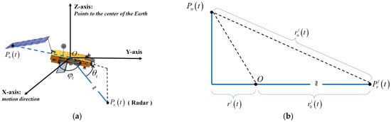
Figure 1.
ISAR imaging geometry of the space target: (a) the observed geometry of the space target; (b) a diagram for constructing the ISAR imaging plane.
Assume that the 3D coordinate of any arbitrary scatterer on the space target is
and the coordinate of the i-th radar is
where represents the range from the geometry center of the target to the i-th radar. Then, the instantaneous range between the i-th radar to scatterer is
Equation (4) can then be expanded via the Taylor series:
In fact, the approximation above has no effect at all on imaging because only the projected range in the LOS direction affects the imaging process. Expanding the plane , as shown in Figure 1b, the instantaneous projected range between the scatterer and the i-th radar in the direction of its LOS is , in which is the projected range from to the i-th LOS:
where is the translational range in the i-th radar. It has no contribution to imaging, and it can be compensated for by the translational compensation algorithm [33,34,35]. After this translational motion compensation, the projected position of scatterer in the direction of the i-th LOS can be obtained, which is also the range coordinate of in the range–Doppler ISAR image of the i-th radar:
where is the initial unit vector of LOS of the i-th radar and is the coordinate of in the BCS. In addition, the instantaneous Doppler frequency of scatterer is the Doppler coordinate in the range–Doppler ISAR image:
Therefore, the projection formula between the 3D geometry of the space target and the multi-view ISAR images can be represented as
where
and where , represents the number of radars, and represents the number of scatterers.
It can be seen from the above analysis that the projection positions of the scatterers in the multi-view ISAR image depend highly on the relative motion of the target to the radars. When the observed target is triaxially stabilized, . If the LOS can be obtained, the geometry of the target can be solved via the ISEA method [30]. When the type of motion of the observed target is known or can be described by some model, can easily be obtained and the geometry of the target can be solved via the method in [31]. However, the motion of the target can be diverse and changed easily, so 3D reconstruction algorithms based on specific target models are limited in real scenarios. In this regard, the EFF is proposed in this paper to solve this problem, and the details are provided in the remaining sections.
2.2. 3D Geometry Reconstruction Method from Multi-View ISAR Images
2.2.1. Multi-View ISAR Images Acquisition
In order to obtain as many multi-view ISAR images of the space target as possible, the space target can be observed through the ISAR network, the observation geometry of which is shown in Figure 2. It is worth emphasizing that the proposed method only requires multi-view ISAR images of space targets as the input. Therefore, there is no need to achieve any form of synchronization or synergia between radars in the network, and each radar can operate completely independently, which greatly reduces the demand for radar resources during observation tasks.
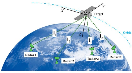
Figure 2.
ISAR observation scenario based on the radar network.
After each radar obtains the echo of the space target, the original data are processed by ISAR imaging. Due to the high speed of the space target relative to the radars, the second-order phase term in these range signals will lead to severe defocusing in the high-resolution range profiles (HRRPs). Therefore, it must be initially well compensated for before high-resolution 2D imaging is performed [36,37,38,39,40]. The method in [41] can solve this problem well. Then, the multi-view ISAR images of the space target can be obtained via the range–Doppler algorithm.
2.2.2. Key Point Extraction and Association
The SFM theory provides that, given the projection positions of four points in a 3D space that are not coplanar from three perspectives, their 3D relative coordinates can be uniquely determined. Therefore, in order to reconstruct the 3D geometry of a space target and its projection vectors, it is necessary to extract at least four key points that are not coplanar in the multi-view ISAR images. However, due to the particularity of the ISAR imaging mechanism, the scatterers in ISAR images are very anisotropic and there are complex scattering characteristics as well, such as sliding scatterers. Moreover, the observation angles can be discretized and discontinuous under the radar network scenario, which fails tracking and association methods based on the scatterer trajectory model.
Fortunately, feature point extraction methods based on deep learning have been widely used in various optical image-processing tasks, such as human pose estimation due to its strong generalization and great performance [42,43,44]. These kinds of deep networks can automatically detect and classify key points of the human body after training on datasets.
Based on the Faster R-CNN [45], the Mask R-CNN [46] takes into account the RoI-Align layer and its branch to generate a mask. It can detect and classify multiple objects in images quickly and accurately and has the ability to generate masks with pixel-level alignment. If the masks that represent the target areas are reduced into one pixel, the positions of the masks represent the locations of the key points, and the categories of the masks represent the indices of the key points. Then, the KeyPoint R-CNN is applied to the key point extraction task to replace the tracking and association process in multi-view ISAR images. The structure of the KeyPoint R-CNN is shown in Figure 3. The feature maps can be obtained through the backbone network consisting of a feature pyramid network (FPN) and ResNet-101. Then, the RoI regions containing the target are proposed via the region proposal network (RPN). After that, the RoI regions are aligned to the corresponding region in the original image via the RoI Align layer, followed by the head networks that generate the positions of key points and corresponding masks. It is worth noting that for targets with different backbone structures, it is necessary to set different key point annotations and to train the networks separately.
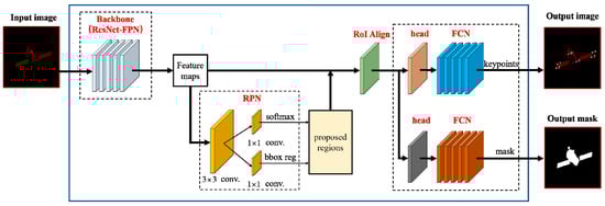
Figure 3.
The structure of the KeyPoint R-CNN.
Assume that the coordinates of key points from different views are
Then, it is noted that the errors caused by the biases in range and angle between the multiple radars will lead to misalignment of the geometric center of the target in the multi-view ISAR images, which in turn affects the accuracy of the 3D reconstruction algorithm. To this end, the geometric center of the extracted scatterers in each frame of an ISAR image can be aligned by subtracting the mean values of the scatterers’ positions from the positions of each extracted scatterer in each frame of the ISAR image:
where is the mean position of the scatterers in the f-th ISAR image. In this way, the origin of the reconstructed coordinate system is the geometric center of the 3D positions of the scatterers, eliminating the error influence of the range and angle measurements.
In order to construct the range–Doppler (RD) measurement matrix, the horizontal and vertical coordinates of the extracted key points need to be converted into the range and Doppler, respectively:
where is a matrix, in which all the elements are 1. and represent the range resolution unit and the Doppler resolution unit in the RD images that can be calculated through the radar’s working parameters, respectively, and the symbol ‘’ represents the Hadamard product.
Moreover, the masks of the target obtained from the KeyPoint R-CNN can also be used as prior information in two aspects in the proposed algorithm. On one hand, the multi-view ISAR images can be denoised by reducing the energy outside the mask region of the target. On the other hand, the masks can be used as the projected images to improve the reconstructed point cloud. The details will be introduced in the following sections.
ISAR imaging is based on the scattering point model because ISAR works in the microwave band. The scattering characteristics of electromagnetic waves in the microwave band are quite different from those in the visible light band, and the back-scattering characteristics of structures, such as metal surfaces, optical windows, cables, and wires, are quite different in ISAR images from different views. These scattering parts are considered the unstable scattering parts. However, there are still stable scattering points on the target, such as the corner points of the satellite solar panels and the end points of the antennas on the cabin, and their scattering characteristics are always stable, so long as they are not occluded. Therefore, the KeyPoint R-CNN mainly extracts these stable scatterers. On the other hand, these stable scatterers are most likely non-coplanar because the four corner points of the satellite solar panels are always coplanar, and the other stable scatterers are usually on different parts of the satellite. Therefore, these scatterers are usually manually extracted first in several 2D ISAR images, and the number of images must be greater than three, according to the SFM theory. Then, the RD measurement matrix can be formed, with which the eigenvalues can be calculated. If the third largest eigenvalue is much larger than the fourth one, then the extracted scatterers are considered non-coplanar. Otherwise, another stable scatterer is chosen to satisfy the above condition. The specific principle will be introduced in Section 2.2.3.
2.2.3. Projection Vector Construction
The SFM theory is only necessary to decompose the range measurement matrix of the target to obtain the 3D coordinates of the scatterers of the target. However, the projection vectors decomposed from the Doppler measurement matrix are also needed to recover the dense point cloud of the target. Therefore, this section proposes an improved factorization method, with which the range–Doppler measurement matrix of several key points can be factorized into the product of their 3D coordinates and the projection vectors.
The RD measurement matrix of the extracted key points can be rewritten via Equations (13) and (15) as follows:
where represents the horizontal coordinates of the extracted key points, i.e., the Doppler measurements of the key points relative to the center of the turntable, and represents the vertical coordinates of the extracted key points, i.e., the range measurements of the key points relative to the center of the turntable.
The imaging plane of the f-th ISAR image is determined by and , in which the vector represents the vertical range axis, while the vector is the horizontal Doppler axis. Therefore, Equation (9) can be expressed as the discrete matrix form:
where
In the presence of noise, according to rank deficient theory, the RD measurement matrix can be decomposed via singular value decomposition (SVD) as
where and . and are the matrices consisting of the corresponding eigenvector. Therefore, there exist and such that
However, the above decomposition is not unique as, for any arbitrary invertible matrix, , stands. In this regard, the following restraints are introduced:
Unlike the traditional factorization method, the above equations do not constrain the Doppler projection vector on its modulus. Considering that there exists the unknown motion of the target itself, the effective rotating axis and the effective angular velocity of rotation can hardly be determined, leading to inaccurate cross-range scaling. Therefore, the RD measurement matrix used in the proposed method consists of the Doppler measurements of key points, which eliminates the errors from the inaccurate cross-range scaling. According to the ISAR imaging turntable model, the cross-range projection vector can be expressed as
where ‘’ represents the cross product of vectors. Furthermore, the magnitude of the Doppler measurement of the key points in the images is . Therefore, the Doppler projection vector is a non-unit vector orthogonal to the range projection vector .
Let
and the constrains in Equation (22) be represented as
where
Therefore, we have
Then, matrix can be obtained from . Under the condition that satisfies the positive definite matrix, matrix can be calculated based on Cholesky decomposition. Therefore, the 3D coordinates of the key points and the projection vectors can be represented as
Until now, the traditional factorization method has only obtained the 3D coordinates of extracted key points and, as mentioned above, due to the complex scattering characteristics of ISAR images, the number of feature points that can be stably extracted and associated in the multi-view ISAR images is small, which hardly reflects the overall geometry of the target. However, the proposed EFF makes full use of the decomposed projection matrix to solve the dense 3D point cloud of the target. The specific steps are set out below.
2.2.4. 3D Geometry Reconstruction
As indicated by the above discussion, the projection vectors from the 3D coordinates of scatterers and the multi-view ISAR images can be obtained. In the absence of noise, after projection onto the 2D ISAR image plane via , a true 3D scatterer on the surface of the target will lie in the 2D target’s region in most multi-view ISAR images and show higher energy than false scatterers. Based on this, 3D imaging of targets can be transformed into an unconstrained optimization problem of searching for 3D positions that have more projected accumulation energy. Therefore, the reconstructed 3D positions can be represented as
where represents the candidate 3D positions; is the f-th real-numbered ISAR image; and are the range resolution unit and the Doppler resolution unit of , respectively; and and are the number of range bins and cross-range bins of , respectively.
To solve the above problem, this section introduces an iterative process via the QPSO algorithm. After one 3D position is obtained, the CLEAN algorithm is used to set the energy of the corresponding projected 2D positions to zeros and to continue the iteration. The specific steps are shown in Algorithm 1.
| Algorithm 1: 3D Reconstruction Method from Multi-View ISAR Images. |
|
It can be seen from the above process that, since the proposed method transforms the 3D geometry reconstruction problem into an unconstrained optimization problem, except for the stable key scattering points, there is actually no strict one-to-one correspondence between the rest of the scattering points and the real scattering points on the target. However, with the exception of cavity scattering and occlusion, any unstable scattering point can be projected onto the target’s area in all multi-view ISAR images, which leads to higher energy than background noise. The proposed method takes the accumulated energy of a candidate scattering point at the projection position in the multi-view ISAR images as the criterion for judging whether it is a true scattering point, so it also has a relatively stable 3D imaging ability for unstable scattering points.
2.2.5. Algorithm Flowchart
The flowchart of the proposed algorithm is summarized in Figure 4. The high-resolution multi-view ISAR images of the space target should first be obtained from the echoes received by the radar networks. Then, the multi-view ISAR images are used as the input of the EFF, in which the key points in images can be extracted and annotated via the well-trained KeyPoint R-CNN. After this, the RD measurement matrix can be obtained. By decomposing the RD measurement matrix via SVD and combining the constraints in Equation (22), the projection vectors from the 3D geometry of the space target to the multi-view ISAR images can be obtained. Finally, after transforming the 3D geometry reconstruction problem into an unconstrained optimization problem, the dense 3D point cloud of the space target can be obtained by finding positions that occupy the most accumulated projection energy.
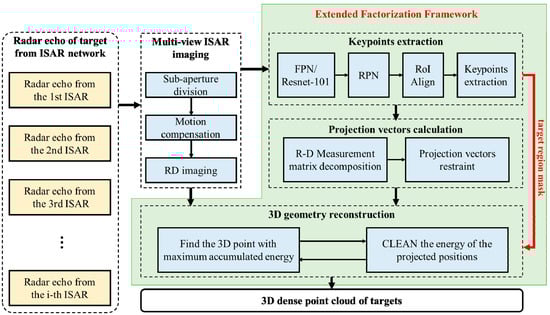
Figure 4.
Flowchart of the proposed method.
2.3. Performance Analysis
2.3.1. Root-Mean-Square Error
The root-mean-square error (RMSE) of the reconstructed 3D geometry can be defined as
where represents the number of the scatterers, denotes the reconstructed 3D coordinates of the n-th scatterer, and is the true position of the n-th scatterer. RMSE reflects the error between the reconstructed points and the ground truth ones.
2.3.2. The Reconstruction Accuracy and Integrity
To better evaluate the accuracy of the reconstructed 3D geometry, appropriate 3D cube grids should first be constructed. As shown in Figure 5, the 3D space in which the space target lies can be divided into a series of small cube grids. The side length of each cube is defined as 20% of the length of the true geometry’s shortest dimension. The number of cube grids must be selected to guarantee that the 3D geometry is completely covered by the envelope of all cube grids.
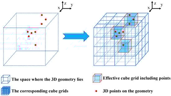
Figure 5.
Diagram of the process for dividing the 3-D space in which the target lies into corresponding cube grids.
Then, we can count the number of small cube grids and occupied by the ground truth point cloud and the reconstructed point cloud, respectively. Finally, the number of common cube grids occupied both by the ground true 3D point cloud and the reconstructed 3D point cloud is counted as . Therefore, the reconstruction accuracy of the reconstructed point cloud is defined as
and the reconstruction integrity is defined as
3. Results
In order to evaluate the performance of the proposed method, four experiments based on simulated electromagnetic data and measured data were carried out, as discussed in the following subsections.
3.1. Effectiveness Validation
The effectiveness of the proposed method was validated by selecting three kinds of satellites for which the skeletons are quite different, i.e., the Hubble Space Telescope (HST), Aqua, and Tiangong-1. The 3D geometries and their corresponding ground truth 3D point clouds are shown in Figure 6, from which we can determine that the key point models of the KeyPoint R-CNN must be distinguished to ensure the performance of the deep networks. As is well known, the points on the solar panels and the points at the edge of the geometries are obvious at most observation angles. Therefore, the six non-coplanar points shown in Figure 6a–c were selected as the key points, where the red numbers represent the indexes of the selected key points. Moreover, the three satellites were in different motion states, where the HST was triaxial stabilized, Aqua is rotating around a fixed axis with constant angular velocity, and Tiangong-1 was rotating around a variant axis with variant angular velocities. The specific motion parameters are shown in Table 1. The out-of-control Tiangong-1 kept rotating with a rotational speed of no more than 3 deg/s before ending its tasks and re-entering the atmosphere, so we set the maximum rotational speed of the above unstable satellites to 3 deg/s, i.e., 0.0524 rad/s.
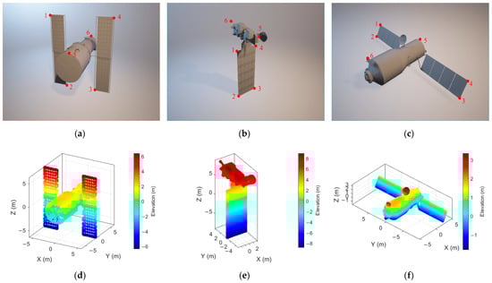
Figure 6.
The 3D geometries and corresponding ground truth 3D point clouds of (a,d) HST, (b,e) Aqua, and (c,f) Tiangong-1.

Table 1.
The motion parameters of different targets.
In order to obtain multi-view ISAR images for the reconstruction task, four radars were considered in this scenario and they were distributed in different directions from the target. The center frequencies of the simulated radars were 10 Ghz; i.e., the radars were working in the X band. The bandwidths of the transmitted signals were all 2 GHz. Therefore, the wavelengths of the transmitted signals were 0.03 m. In addition, the minimum dimension of the three targets was no less than 4 m, while the maximum dimension was no more than 20 m. Therefore, the sizes of the targets were much larger than the wavelengths of the transmitted signals, leading to the three targets being categorized as electrically large objects. Physical Optics (PO) is an excellent method in the field of high-frequency electromagnetic field calculation [47]. For electrically large objects, the PO method can give satisfactory results, while having a fast calculation speed and requiring little memory. Therefore, the simulated electromagnetic echoes of the targets were obtained via the PO method. The 12,500 echoes obtained by each radar were divided into 96 sub-apertures, and the improved RD imaging method was utilized to generate the high resolution ISAR images. Three of each of them are shown in Figure 7a1–c3, where the white dots are the extracted key points corresponding to the ones shown in Figure 6a–c, while the white numbers are the corresponding indices.
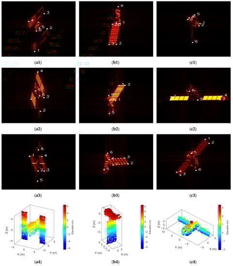
Figure 7.
The 2D ISAR images and corresponding key points extraction of (a1–a3) HST, (b1–b3) Aqua, and (c1–c3) Tiangong-1, as well as the reconstructed 3D point clouds of (a4) HST, (b4) Aqua, and (c4) Tiangong-1.
To train the KeyPoint R-CNN, for each satellite, 5000 ISAR images from different views were obtained as the dataset, 90% of which were used as the training dataset, while the remaining 10% were used as the validation dataset. We set the learning rate as 0.02 and trained the KeyPoint R-CNN for 100 iterations on a single 2080Ti for 8 h.
By using the proposed EFF, the six key points were reconstructed, followed by the D geometry reconstruction of HST, Aqua, and Tiangong-1. The reconstructed 3D point clouds are shown in Figure 7a4,b4,c4, respectively. Then, using Equations (31)–(33), the RMSEs, the reconstruction accuracies, and the reconstruction integrities were calculated, as listed in Table 2, which shows the effectiveness of the proposed method. Moreover, it is noted that the reconstruction integrity of Tiangong-1 is smaller than that of HST and Aqua, which is mainly caused by the cabin of Tiangong-1′s CAD model being much smoother, leading to lower energy in the multi-view ISAR images. Therefore, the reconstructed 3D point cloud of Tiangong-1 had fewer points on the cabin part. However, compared with the ground truth 3D point clouds of the satellites shown in Figure 6d–f, the reconstructed 3D point clouds of these satellites still showed high accuracy and high integrity.
Table 2.
The evaluation values of the reconstructed geometries.
3.2. Comparison Analysis
As discussed in this subsection, the electromagnetic data of the above three satellites were used to validate the advantages of the proposed method. For comparison purposes, only the data in one observation from a single radar were utilized. As illustrated in the previous subsection, the three satellites were in different motion states; the specific parameters are shown in Table 1.
In a similar manner, the 12,500 echoes ere then divided into 96 sub-apertures, and 96 frames of ISAR images were obtained via the improved RD algorithm. Then, the 3D geometries of HST, Aqua, and Tiangong-1 were reconstructed via the ISEA method [30], the 3D geometry reconstruction method for SRST [31], and the proposed method, as shown in Figure 8. It can easily be seen that the scenarios that the three methods can handle are quite different. Specifically, the ISEA method can reconstruct the 3D point cloud only when the target is triaxial stable, while the method in [31] can obtain the 3D point clouds of the target when it is triaxial stable or slowly rotating. However, when the motion parameters start to change, i.e., the target is non-stationarily rotating, the projection relationship is invalidated, making the ISEA method and the method in [31] less effective. It is obvious that these two methods are highly sensitive to the motion of the target: when the motion state of the target no longer obeys the pre-set one, the performance of these two methods decreases significantly. Therefore, the proposed method can obtain the 3D point clouds of the targets in all the above scenarios, showing its high robustness.
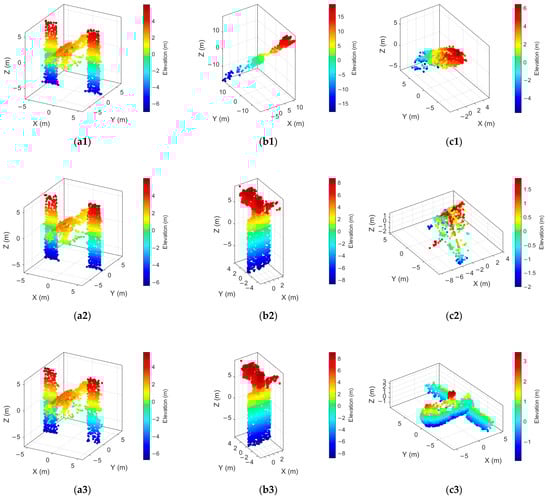
Figure 8.
The reconstructed 3D point clouds of HST, Aqua, and Tiangong-1 via (a1–c1) the method in [30], (a2–c2) the method in [31], and (a3–c3) the proposed method.
By calculating the reconstruction accuracy and the reconstruction integrity of the reconstructed 3D point clouds shown in Figure 8, the conclusions above become more obvious. It can easily be concluded from Figure 9a that when the target is triaxial stable, the three methods mentioned above can obtain good performances during a reconstruction task. Furthermore, the reconstruction accuracy of the proposed method is best. In Figure 9b, because Aqua is a slowly rotating target, the ISEA method cannot continue to reconstruct its 3D point cloud using only the LOS information. Therefore, the performance of the ISEA method is the poorest. In contrast, the method in [31] estimated the rotational parameters of Aqua, which were used to modify the projection relationship and to obtain an accurate 3D point cloud. In Figure 9c, Tiangong-1 is non-stationarily rotating, which invalidates the first two methods. However, thanks to the high robustness of the KeyPoint R-CNN, the calculated projection vectors were accurate, resulting in the proposed method being insensitive to the motion of targets. Therefore, a high and stable performance throughout the entire experiment was shown.
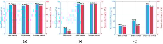
Figure 9.
The reconstruction accuracies and integrities of different methods on (a) HST, (b) Aqua, and (c) Tiangong-1.
3.3. Statistical Analysis
To better validate the robustness of the proposed method, Monte Carlo simulations were implemented by taking into account the number of images used for reconstruction, the signal-to-noise ratio (SNR), and the targets’ motion. In order to eliminate the influence of the model on the experimental results, we used the same model, the HST, in different motion states, i.e., (a) triaxially stable, (b) slowly rotating and (c) non-stationarily rotating. The corresponding motion parameters are shown in Table 1.
In order to validate the robustness of the number of images of the proposed method, the number of ISAR images used for reconstruction was set as 50, 100, 150, 200, 250, 300, and 350. Under each condition, 20 Monte Carlo simulations were implemented. Using the proposed EFF, the evaluation values of the reconstructed results are shown in Figure 10a–c, from which it can be concluded that the more ISAR images that are used for reconstruction, the better the results. Specifically, the RMSE decreases as the number of images increases, while the reconstruction accuracy and the reconstruction integrity increase as the number of images increases. It is noted that since each set of images selected in the experiment was selected uniformly from ISAR images generated by the four radars, the multi-view information provided by the first 50 ISAR images already contained most of the views required for the 3D reconstruction of the target, and the performance improvement was not very large when additional images were used.
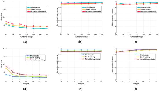
Figure 10.
The (a) RMSEs, (b) reconstruction accuracies, and (c) reconstruction integrities when using different numbers of ISAR images when the HST is in different motion states. The (d) RMSEs, (e) reconstruction accuracies, and (f) reconstruction integrities when using different SNRs of ISAR images when the HST is in different motion states.
Moreover, to validate the robustness on the SNRs of the ISAR images of the proposed method, the SNRs of the ISAR images used for reconstruction were set as 0 dB, 5 dB, 10 dB, 15 dB, 20 dB, 25 dB, and 30 dB. Under each condition, 20 Monte Carlo simulations were implemented. Using the proposed EFF, the evaluation values of the reconstructed results are shown in Figure 10d–f, from which it can be concluded that the higher the SNRs of the ISAR images, the better the results. Therefore, when the SNRs of the ISAR images were higher than 5 dB, the proposed method showed good performance with an RMSE under 0.05 m, and the reconstruction accuracies and integrities were greater than 90%. This indicated that the proposed method is robust to noise in the ISAR images and stays effective in low SNR conditions.
Furthermore, the motion states of the HST can also slightly influence the reconstruction results. This is mainly because the training datasets were not large enough to provide sufficient features for the KeyPoint R-CNN to learn. The projections of rotating targets in ISAR images change more than those of the triaxial stable target, which is why it needed more training data when the targets were unstable. However, the performance of the proposed method always remained at a high, with the RMSEs smaller than 0.05 m, and the reconstruction accuracies and integrities were higher than 90% when the SNRs of the image were higher than 5 dB and the number of ISAR images used was higher than 200.
3.4. Validation on Measured Data
In order to validate the performance of the proposed method on the measured data, the measured ISAR images of Tiangong-1 obtained by the German tracking and imaging radar (TIRA) were adopted to the 3D reconstruction experiment. The data were recorded when Tiangong-1 was about to re-enter the atmosphere, so it was uncontrolled and in a non-stationarily rotating state. The ISAR images were captured from the video published on the official website of the Fraunhofer Institute for High Frequency Physics and Radar Techniques (FHR) [48]. By capturing each frame of the published video file, 840 frames of ISAR images could be obtained, of which 140 frames were randomly picked as the source data for the reconstructing task. The remaining images were used as the training dataset for the KeyPoint R-CNN. Two frames of the ISAR images and the corresponding key points extracted by the KeyPoint R-CNN are shown in Figure 11a,b, where the white dots and numbers in the ISAR images represent the extracted key points and corresponding indexes. After obtaining the positions of the key points in the ISAR image sequence, the proposed method was used to recover the 3D geometry of Tiangong-1, and the result is shown in Figure 11c. It can be noticed that the main body (cabin) and the solar panels can be easily distinguished from the reconstructed 3D geometry, which shows the performance of the proposed method. Nevertheless, because the ISAR image sequence were captured from video, the resolution could not be determined accurately. Therefore, the size of the reconstructed geometry was inaccurate.
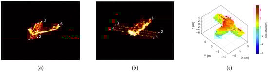
Figure 11.
ISAR images and the reconstructed 3D geometry of Tiangong-1. (a) the first frame and (b) the sixty-fourth frame of the ISAR image sequence, and (c) the reconstructed 3D geometry of Tiangong-1.
Except for the data of the satellite, other measured data for an aircraft Yak-42 were used to validate the effectiveness and robustness of the proposed method. The measured data were recorded via a test C-band radar with a 0.4 GHz bandwidth. The 20000 echoes were divided into 618 sub-apertures, and 618 frames of ISAR images were obtained via the improved RD algorithm, 34 frames of which were used to reconstruct the 3D geometry of Yak-42, while the remaining images were used as the training dataset and the testing dataset. The endpoints of the nose, wings, and tails of Yak-42 were regarded as the key points. The third and the fourteenth frames of ISAR image and the extracted key points are shown in Figure 12ab, where the white dots and numbers in the ISAR images represent the extracted key points and corresponding indexes. Using the proposed method, five key points, followed by the 3D geometry, were reconstructed. The reconstructed 3D point cloud of Yak-42 is shown in Figure 12c, from which it can be noticed that the 3D geometry of Yak-42 is clear and the fuselage, the wings, and the tails can easily be distinguished. Moreover, the fuselage length and the wingspan of Yak-42 were 36.38 m and 34.88 m, respectively [49]. By measuring the corresponding sizes of the reconstructed 3D point cloud, the estimated values of the fuselage length and the wingspan were 33.55 m and 37.63 m, respectively. Therefore, the percentages of estimation errors for fuselage length and the wingspan were 7.77% and 7.90%, respectively, showing that the proposed method has good performance.
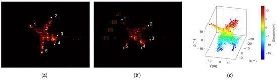
Figure 12.
ISAR images and the reconstructed 3D geometry of Yak-42. (a) The first frame and (b) the fourteenth frame of the ISAR image sequence, and (c) the reconstructed 3D geometry of Yak-42.
4. Discussion
Thanks to the KeyPoint R-CNN, the proposed EFF is effective in more general scenarios. The experiments in the above subsections show the effectiveness and robustness of the proposed EFF and indicate that it can easily handle scenarios where space targets are triaxially stable, slowly rotating, or non-stationarily rotating. Moreover, it is obvious that the proposed EFF can be used not only in the 3D geometry reconstruction of space targets from ISAR images, but also in the 3D geometry reconstruction of any kind of targets from all kinds of images, so long as there are stable key points and the energy of the targets in the images are much larger than that in the background.
5. Conclusions
The main goal of ISAR is to observe uncooperative targets from very far distances. The real size of the targets can hardly be estimated from ISAR images, due to their unexpected motion relative to the radar. This is why 3D geometry reconstruction is needed and why the traditional factorization method cannot be used in ISAR images directly. To this end, our previous works proposed some 3D geometry reconstruction methods for triaxially stable space targets and slowly rotating space targets. However, these previous methods could only be used in scenarios where the targets’ motion states were strictly followed by specific models, which greatly limited its applications in practice. As an extension of these previous methods, the proposed EFF in this paper uses the KeyPoint R-CNN to extract a small number of key points to form the range–Doppler measurement matrix. Then, the 3D coordinates of the key points and the projection vectors can be solved via the modified factorization method, in which the constrains are updated to adapt to the range–Doppler ISAR images. Furthermore, to obtain a more complete 3D geometry of the targets, more scatterers on the geometry of targets can be solved by utilizing the projection vectors. However, due to the high energy of the cavity-scattering parts of the target in multi-view ISAR images, the proposed method cannot distinguish them from real scatterers on the target, which leads to some false-alarm structures in the 3D geometry reconstruction result.
Moreover, the KeyPoint R-CNN in the EFF is a data-driven neural network, so large amounts of well-focused ISAR images from different observation views with labels are necessary to train such a network. However, in real scenarios, space targets always operate in specific orbits, resulting in a long time taken to accumulate enough images from different views for the same target. Moreover, the multi-view ISAR images obtained from multiple radars are not labeled, so generating accurate labels for each image is another time-costly task. However, once the KeyPoint R-CNN for a particular target has been well-trained, the subsequent key point detection process can be finished quickly and accurately. On the other hand, if there are few labeled data, the accuracy of the extraction will decrease. Fortunately, as a key point extractor in the EFF, the KeyPoint R-CNN can be changed into any method that can acquire the 2D positions of key points. These methods, as a substitute for KeyPoint R-CNN, can be regarded as the activations of the EFF when the observation dataset is small in the beginning.
Author Contributions
Conceptualization, Z.Z.; formal analysis, Z.Z.; funding acquisition, L.L. and F.Z.; methodology, Z.Z. and L.L.; project administration, Z.Z.; validation, Z.Z.; visualization, Z.Z.; writing—original draft, Z.Z.; writing—review and editing, Z.Z., L.L., X.J. and F.Z. All authors have read and agreed to the published version of the manuscript.
Funding
This work was supported in part by the National Natural Science Foundation of China under grant no. 62001350, in part by the China Postdoctoral Science Foundation under grant no. 2020M673346, in part by the Postdoctoral Science Research Projects of Shaanxi Province, in part by the Fundamental Research Funds for the Central Universities, and in part by the Innovation Fund of Xidian University.
Data Availability Statement
Not applicable.
Acknowledgments
The authors thank the anonymous reviewers for their valuable suggestions, which were of great help in improving the quality of this paper.
Conflicts of Interest
The authors declare no conflict of interest.
References
- Fonder, G.; Hughes, M.; Dickson, M.; Schoenfeld, M.; Gardner, J. Space fence radar overview. In Proceedings of the 2019 International Applied Computational Electromagnetics Society Symposium (ACES), Miami, FL, USA, 14–19 April 2019; pp. 1–2. [Google Scholar]
- Anger, S.; Jirousek, M.; Dill, S.; Peichl, M. IoSiS—A high performance experimental imaging radar for space surveillance. In Proceedings of the 2019 IEEE Radar Conference (RadarConf), Boston, MA, USA, 22–26 April 2019; pp. 1–4. [Google Scholar]
- Kang, L.; Liang, B.S.; Luo, Y.; Zhang, Q. Sparse imaging for spinning space targets with short time observation. IEEE Sens. J. 2021, 21, 9090–9098. [Google Scholar] [CrossRef]
- Luo, X.; Guo, L.; Shang, S.; Song, D.; Li, X.; Liu, W. ISAR imaging method for non-cooperative slow rotation targets in space. In Proceedings of the 2018 12th International Symposium on Antennas, Propagation and EM Theory (ISAPE), Hangzhou, China, 3–6 December 2018; pp. 1–4. [Google Scholar]
- Liu, M.; Zhang, X. ISAR imaging of rotating targets via estimation of rotation velocity and keystone transform. In Proceedings of the 2017 IEEE Conference on Antenna Measurements & Applications (CAMA), Tsukuba, Japan, 4–6 December 2017; pp. 265–267. [Google Scholar]
- Tian, X.; Bai, X.; Xue, R.; Qin, R.; Zhou, F. Fusion recognition of space targets with micromotion. IEEE Trans. Aerosp. Electron. Syst. 2022, 58, 3116–3125. [Google Scholar] [CrossRef]
- Ma, C.; Zhang, S. Applications of super resolution signal processing on monopulse radar three dimensional imaging. J. Xidian Univ. 1999, 26, 379–382. [Google Scholar]
- Li, H.; Ding, L. Research on monopulse 3-D imaging tests. J. Spacecr. TTC Technol. 2010, 29, 74–78. [Google Scholar]
- Li, J.; Quan, Y.; Xing, M.; Li, H.; Li, Y. 3-D ISAR imaging technology based on sum-diff beam. Chin. J. Radio Sci. 2010, 25, 281–286. [Google Scholar]
- Rong, J.; Wang, Y.; Han, T. Iterative optimization-based ISAR imaging with sparse aperture and its application in interferometric ISAR imaging. IEEE Sens. J. 2019, 19, 8681–8693. [Google Scholar] [CrossRef]
- Wang, G.; Xia, X.; Chen, V. Three-dimensional ISAR imaging of maneuvering targets using three receivers. IEEE Trans. Image Process. 2001, 10, 436–447. [Google Scholar] [CrossRef]
- Liu, Y.; Song, M.; Wu, K.; Wang, R.; Deng, Y. High-quality 3-D InISAR imaging of maneuvering target based on a combined processing approach. IEEE Geosci. Remote Sens. Lett. 2013, 10, 1036–1040. [Google Scholar] [CrossRef]
- Xu, G.; Xing, M.; Xia, X.; Zhang, L.; Chen, Q.; Bao, Z. 3D geometry and motion estimations of maneuvering targets for interferometric ISAR with sparse aperture. IEEE Trans. Image Process. 2016, 25, 2005–2020. [Google Scholar] [CrossRef] [PubMed]
- Kang, L.; Luo, Y.; Zhang, Q.; Liu, X.; Liang, B. 3-D scattering image sparse reconstruction via radar network. IEEE Trans. Geosci. Remote Sens. 2021, 60, 1–14. [Google Scholar] [CrossRef]
- Kang, L.; Luo, Y.; Zhang, Q.; Liu, X.; Liang, B. 3D scattering image reconstruction based on measurement optimization of a radar network. Remote Sens. Lett. 2020, 11, 697–706. [Google Scholar] [CrossRef]
- Liu, X.; Zhang, Q.; Jiang, L.; Liang, J.; Chen, Y. Reconstruction of three-dimensional images based on estimation of spinning target parameters in radar network. Remote Sens. 2018, 10, 1997. [Google Scholar] [CrossRef]
- Xu, D.; Xing, M.; Xia, X.; Sun, G.; Fu, J.; Su, T. A multi-perspective 3D reconstruction method with single perspective instantaneous target attitude estimation. Remote Sens. 2019, 11, 1277. [Google Scholar] [CrossRef]
- Zhou, C.; Jiang, L.; Yang, Q.; Ren, X.; Wang, Z. High precision cross-range scaling and 3D geometry reconstruction of ISAR targets based on geometrical analysis. IEEE Access 2020, 8, 132415–132423. [Google Scholar] [CrossRef]
- Liu, L.; Zhou, F.; Bai, X.; Tao, M.; Zhang, Z. Joint cross-range scaling and 3D geometry reconstruction of ISAR targets based on factorization method. IEEE Trans. Image Process. 2016, 25, 1740–1750. [Google Scholar] [CrossRef]
- Ullman, S. The Structure from Motion Theorem; MIT Press: Cambridge, MA, USA, 1979. [Google Scholar]
- Leutenegger, S.; Chli, M.; Siegwart, R. BRISK: Binary robust invariant scalable keypoints. In Proceedings of the International Conference on Computer Vision (ICCV), Barcelona, Spain, 6–13 November 2011. [Google Scholar]
- Di, G.; Su, F.; Yang, H.; Fu, S. ISAR image scattering center association based on speeded-up robust features. Multimed. Tools. Appl. 2020, 79, 5065–5082. [Google Scholar] [CrossRef]
- Yang, S.; Jiang, W.; Tian, B. ISAR image matching and 3D reconstruction based on improved SIFT method. In Proceedings of the 2019 International Conference on Electronic Engineering and Informatics (EEI), Nanjing, China, 8–10 November 2019; pp. 224–228. [Google Scholar]
- Lucas, B.; Kanade, T. An iterative image registration technique with an application to stereo vision. In Proceedings of the the 7th International Joint Conference on Artificial Intelligence (IJCAI 81), Vancouver, BC, Canada, 24–28 August 1981; pp. 674–679. [Google Scholar]
- Shi, J.; Tomasi, C. Good features to track. In Proceedings of the IEEE Conference on Computer Vision & Pattern Recognition, Seattle, WA, USA, 21–23 June 1994; pp. 593–600. [Google Scholar]
- Liu, L.; Zhou, F.; Bai, X. Method for scatterer trajectory association of sequential ISAR images based on Markov chain Monte Carlo algorithm. IET Radar Sonar Navig. 2018, 12, 1535–1542. [Google Scholar] [CrossRef]
- Du, R.; Liu, L.; Bai, X.; Zhou, F. A new scatterer trajectory association method for ISAR image sequence utilizing multiple hypothesis tracking algorithm. IEEE Trans. Geosci. Remote Sens. 2022, 60, 1–13. [Google Scholar] [CrossRef]
- Bi, Y.; Wei, S.; Wang, J.; Zhang, Y.; Sun, Z.; Yuan, C. New method of scatterers association and 3D reconstruction based on multi-hypothesis tracking. J. Beijing Univ. Aeronaut. Astronaut. 2016, 42, 1219–1227. [Google Scholar] [CrossRef]
- Wang, X.; Guo, B.; Shang, C. 3D reconstruction of target geometry based on 2D data of inverse synthetic aperture radar images. J. Electron. Inf. Technol. 2013, 35, 2475–2480. [Google Scholar] [CrossRef]
- Liu, L.; Zhou, Z.; Zhou, F.; Shi, X. A new 3-D geometry reconstruction method of space target utilizing the scatterer energy accumulation of ISAR image sequence. IEEE Trans. Geosci. Remote Sens. 2020, 58, 8345–8357. [Google Scholar] [CrossRef]
- Zhou, Z.; Liu, L.; Du, R.; Zhou, F. Three-dimensional geometry reconstruction method for slowly rotating space targets utilizing ISAR image sequence. Remote Sens. 2022, 14, 1114. [Google Scholar] [CrossRef]
- Liu, Y.; Yi, D.; Wang, Z. Coordinate transformation methods from the inertial system to the centroid orbit system. Aerosp. Control 2007, 25, 4–8. [Google Scholar]
- Xin, H.; Bai, X.; Song, Y.; Li, B.; Tao, R. ISAR imaging of target with complex motion associated with the fractional Fourier transform. Digit. Signal Process. 2018, 83, 332–345. [Google Scholar] [CrossRef]
- Yang, L.; Xiong, T.; Zhang, L.; Xing, M. Translational motion compensation for ISAR imaging based on joint autofocusing under the low SNR. J. Xidian Univ. 2012, 39, 63–71. [Google Scholar] [CrossRef]
- Liu, L.; Zhou, F.; Tao, M.; Sun, P.; Zhang, Z. Adaptive translational motion compensation method for ISAR imaging under low SNR based on particle swarm optimization. IEEE J. Sel. Top. Appl. Earth Obs. Remote Sens. 2015, 8, 5146–5157. [Google Scholar] [CrossRef]
- Li, D.; Ren, J.; Liu, H.; Yang, Z.; Wan, J.; Chen, Z. A novel ISAR imaging approach for maneuvering targets with satellite-borne platform. IEEE Geosci. Remote Sens. Lett. 2022, 19, 1–5. [Google Scholar] [CrossRef]
- Zhang, B.; Xu, G.; Zhou, R.; Zhang, H.; Hong, W. Multi-channel back-projection algorithm for mmwave automotive MIMO SAR imaging with Doppler-division multiplexing. IEEE J. Sel. Top. Signal Process. 2022. early access. [Google Scholar] [CrossRef]
- Xu, G.; Zhang, B.; Chen, J.; Hong, W. Structured low-rank and sparse method for ISAR imaging with 2-D compressive sampling. IEEE Trans. Geosci. Remote Sens. 2022, 60, 1–14. [Google Scholar] [CrossRef]
- Yuan, Y.; Luo, Y.; Kang, L.; Ni, J.; Zhang, Q. Range alignment in ISAR imaging based on deep recurrent neural network. IEEE Geosci. Remote Sens. Lett. 2022, 19, 1–5. [Google Scholar] [CrossRef]
- Xu, G.; Zhang, B.; Yu, H.; Chen, J.; Xing, M.; Hong, W. Sparse synthetic aperture radar imaging from compressed sensing and machine learning: Theories, applications, and trends. IEEE Geosc. Remote Sen. Mag. 2022, 10, 32–69. [Google Scholar] [CrossRef]
- Fan, H.; Ren, L.; Mao, E.; Liu, Q. A high-precision method of phase-derived velocity measurement and its application in motion compensation of ISAR imaging. IEEE Trans. Geosci. Remote Sens. 2018, 56, 1–18. [Google Scholar] [CrossRef]
- Xiao, B.; Wu, H.; Wei, Y. Simple baselines for human pose estimation and tracking. In Proceedings of the Computer Vision and Pattern Recognition, Munich, Germany, 8–14 September 2018; pp. 472–487. [Google Scholar]
- Sun, K.; Xiao, B.; Liu, D.; Wang, J. Deep high-resolution representation learning for human pose estimation. In Proceedings of the 32nd IEEE/CVF Conference on Computer Vision and Pattern Recognition (CVPR), Long Beach, CA, USA, 16–20 June 2019; pp. 5686–5696. [Google Scholar]
- Cheng, B.; Xiao, B.; Wang, J.; Shi, H.; Huang, T.; Zhang, L. HigherHRNet: Scale-aware representation learning for bottom-up human pose estimation. In Proceedings of the IEEE/CVF Conference on Computer Vision and Pattern Recognition (CVPR), Electr Network, Seattle, WA, USA, 14–19 June 2020; pp. 5385–5394. [Google Scholar]
- Ren, S.; He, K.; Girshick, R.; Sun, J. Faster R-CNN: Towards real-time object detection with region proposal networks. IEEE Trans. Pattern Anal. Mach. Intell. 2017, 39, 1137–1149. [Google Scholar] [CrossRef] [PubMed]
- He, K.; Gkioxari, G.; Dollar, P.; Girshick, R. Mask R-CNN. In Proceedings of the International Conference on Computer Vision, Venice, Italy, 22–29 October 2017; pp. 386–397. [Google Scholar]
- Andrey, V.O.; Sergei, A.T. Method of Physical Optics. In Modern Electromagnetic Scattering Theory with Applications; Wiley: Hoboken, NJ, USA, 2013; pp. 565–633. [Google Scholar]
- Lars, F. Monitoring the Re-Entry of the Chinese Space Station Tiangong-1 with TIRA. Available online: https://www.fhr.fraunhofer.de/en/businessunits/space/monitoring-the-re-entry-of-the-chinese-space-station-tiangong-1-with-tira.html (accessed on 1 April 2018).
- CAAC. Introduction of the Yak-42 Series. Available online: http://www.caac.gov.cn/GYMH/MHBK/HKQJS/201509/t20150923_1871.html (accessed on 23 September 2015).
Disclaimer/Publisher’s Note: The statements, opinions and data contained in all publications are solely those of the individual author(s) and contributor(s) and not of MDPI and/or the editor(s). MDPI and/or the editor(s) disclaim responsibility for any injury to people or property resulting from any ideas, methods, instructions or products referred to in the content. |
© 2023 by the authors. Licensee MDPI, Basel, Switzerland. This article is an open access article distributed under the terms and conditions of the Creative Commons Attribution (CC BY) license (https://creativecommons.org/licenses/by/4.0/).