
High Resolution Fourier Transform Spectrometer for Ground-Based Verification of Greenhouse Gases Satellites
 ,
,  , and
, and
Abstract
1. Introduction
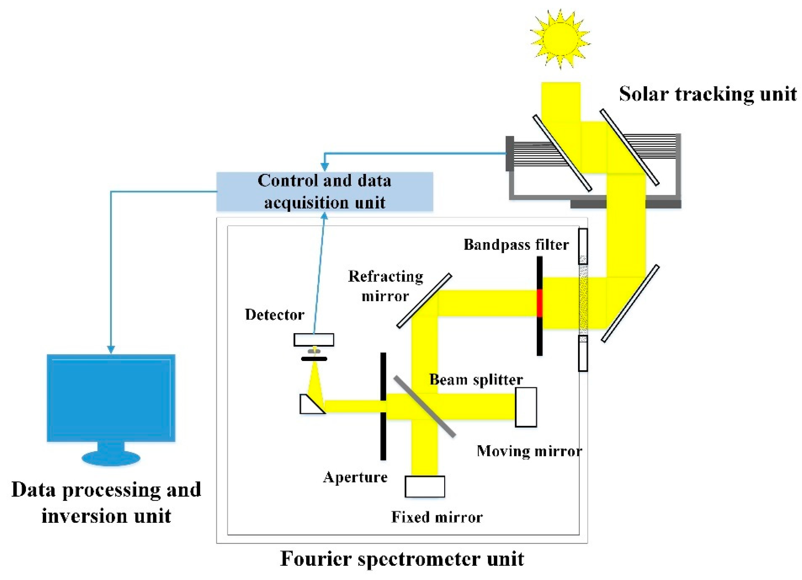
2. Spectrometer
3. Calibration
3.1. Gas Absorption Transmittance
3.2. Instrument Line Shape
4. Methodology
4.1. Spectral Restoration
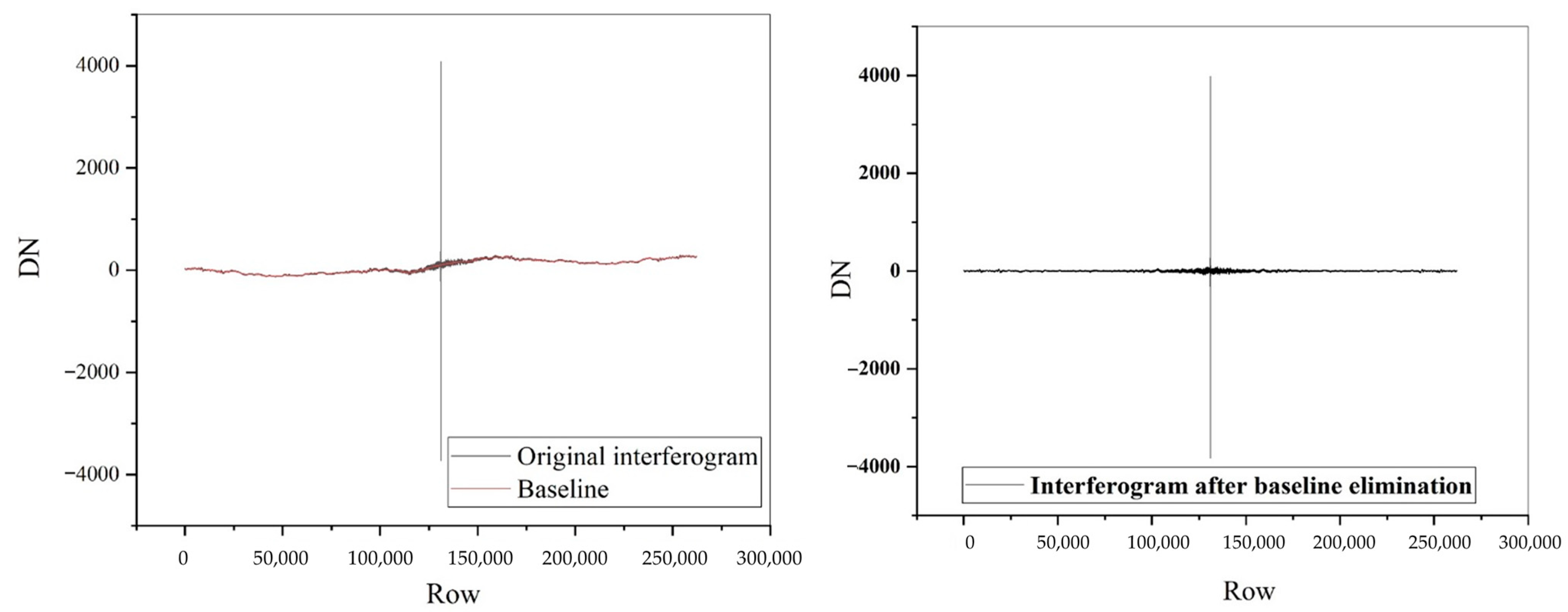
4.1.1. Baseline Correction
4.1.2. Phase Correction
4.1.3. Fourier Transform
4.2. Quality Control
4.2.1. Measuring Interference
4.2.2. Solar Light Fluctuation
4.3. Gas Inversion
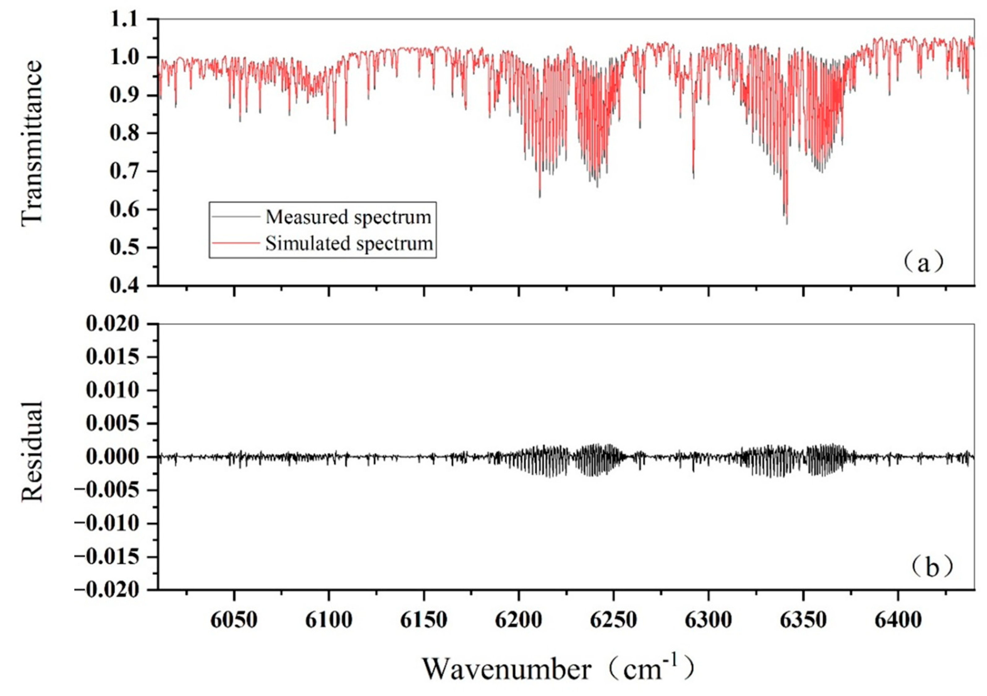
4.3.1. Spectral Correction
- (1)
- Given initial value, , > 0, ε > 0;
- (2)
- Calculation of ;
- (3)
- Calculate according to the LM algorithm expression;
- (4)
- Judge whether is less than ε. If it is less, then end the iteration, otherwise continue with step (5);
- (5)
- If , will increase; if < , will be reduced.
4.3.2. Profiles Reconstruction
4.3.3. Experiment
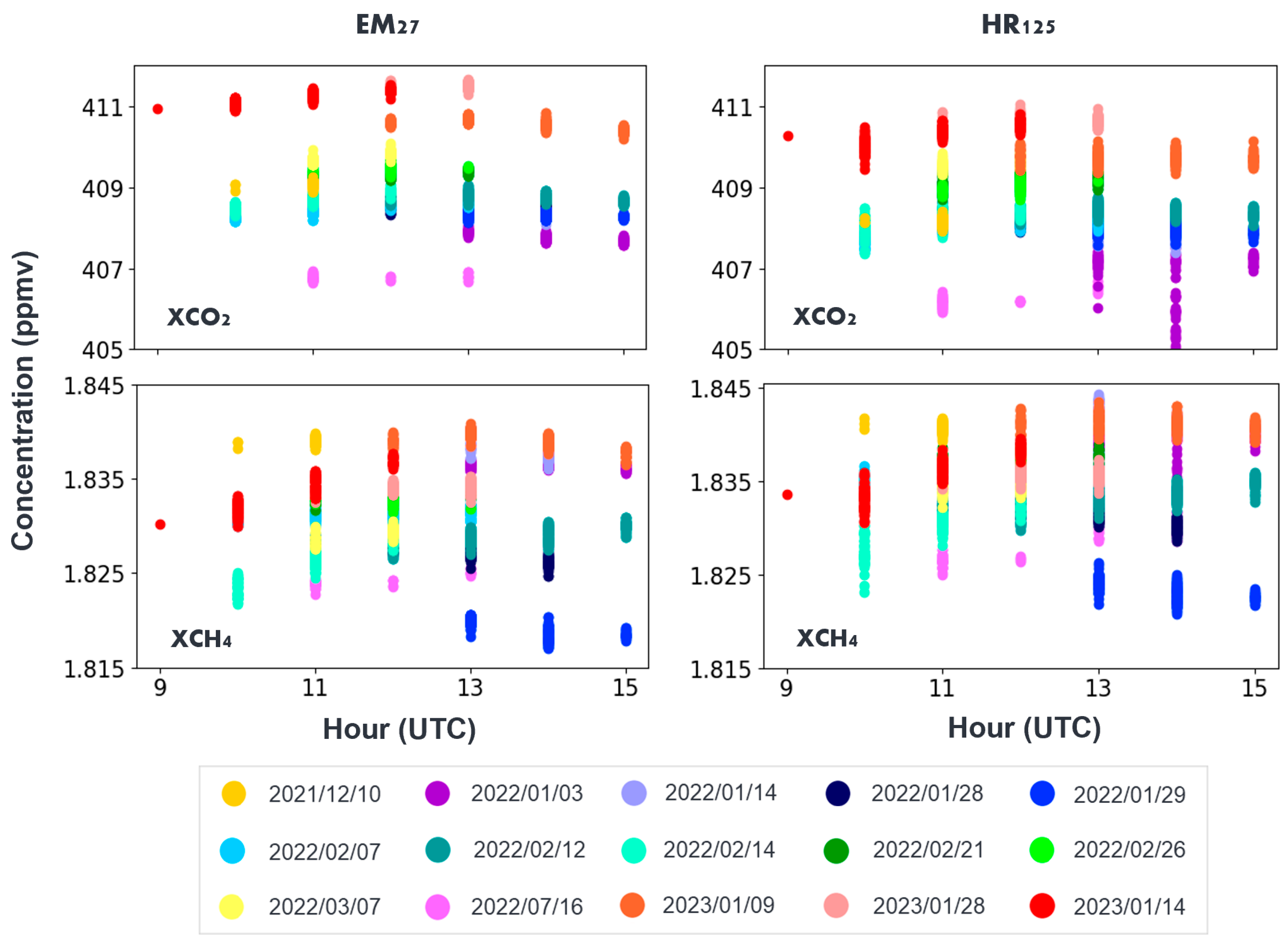
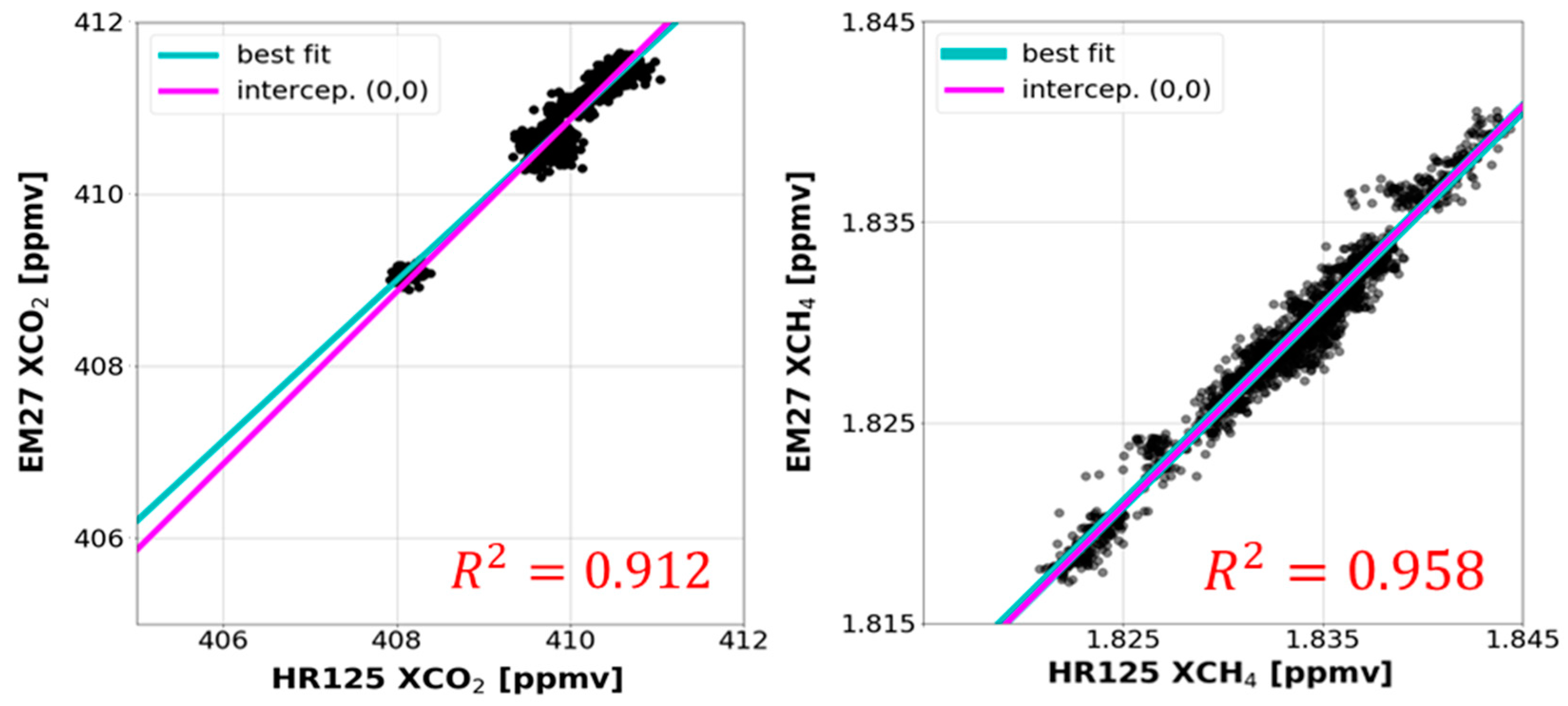
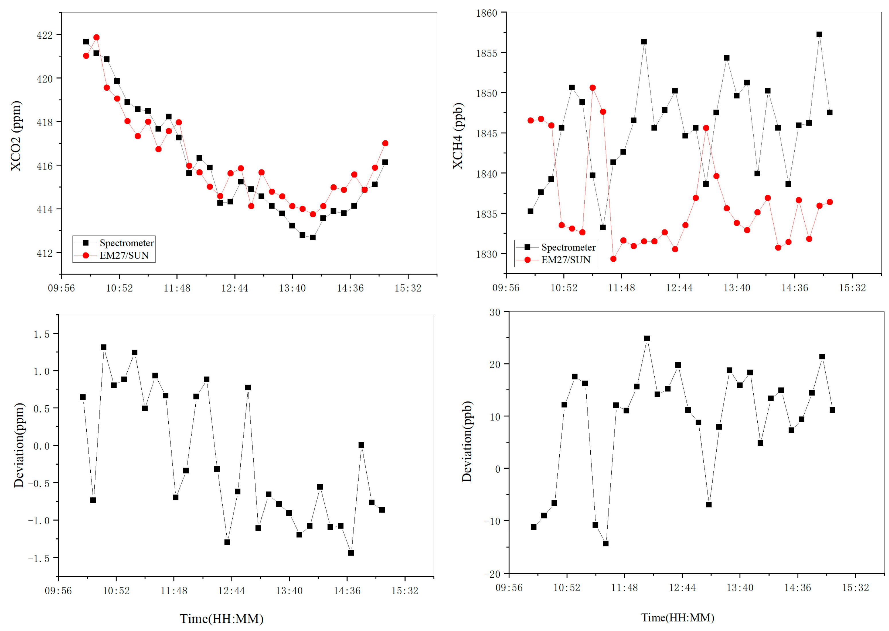
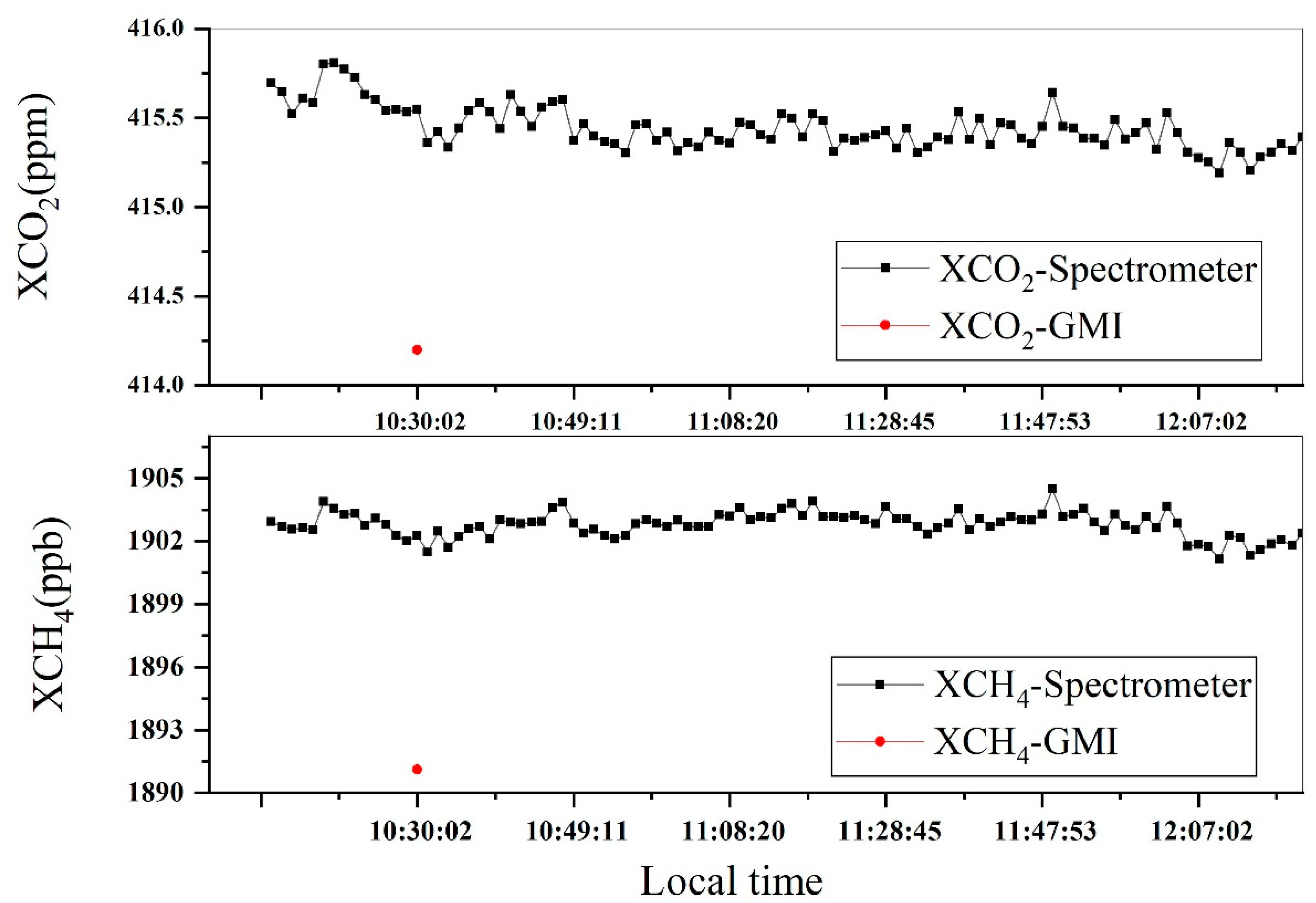
5. Results
6. Conclusions
Author Contributions
Funding
Data Availability Statement
Conflicts of Interest
References
- Rogelj, J.; Den Elzen, M.; Höhne, N.; Fransen, T.; Fekete, H.; Winkler, H.; Schaeffer, R.; Sha, F.; Riahi, K.; Meinshausen, M. Paris Agreement climate proposals need a boost to keep warming well below 2 °C. Nature 2016, 534, 631–639. [Google Scholar] [CrossRef]
- Jiang, K. IPCC Special Report on 1.5 °C Warming: A Starting of New Era of Global Mitigation. Clim. Chang. Res. 2018, 14, 640–642. [Google Scholar]
- Kuze, A.; Suto, H.; Nakajima, M.; Hamazaki, T. Thermal and near infrared sensor for carbon observation Fourier-transform spectrometer on the Greenhouse Gases Observing Satellite for greenhouse gases monitoring. Appl. Opt. 2009, 48, 6716–6733. [Google Scholar] [CrossRef]
- Miller, C.E.; Crisp, D.; DeCola, P.L.; Olsen, S.C.; Randerson, J.T.; Michalak, A.M.; Alkhaled, A.; Rayner, P.; Jacob, D.J.; Suntharalingam, P.; et al. Precision requirements for space-based data. J. Geophys. Res. Atmos. 2007, 112. [Google Scholar] [CrossRef]
- Wang, S.; van der A, R.J.; Stammes, P.; Wang, W.; Zhang, P.; Lu, N.; Zhang, X.; Bi, Y.; Wang, P.; Fang, L. Carbon Dioxide Retrieval from TanSat Observations and Validation with TCCON Measurements. Remote Sens. 2020, 12, 2204. [Google Scholar] [CrossRef]
- Xiong, W. Greenhouse gases Monitoring Instrument(GMI) on GF-5 satellite (invited). Infrared Laser Eng. 2019, 48, 303002. [Google Scholar] [CrossRef]
- Pollard, D.F.; Sherlock, V.; Robinson, J.; Deutscher, N.M.; Connor, B.; Shiona, H. The Total Carbon Column Observing Network site description for Lauder, New Zealand. Earth Syst. Sci. Data 2017, 9, 977–992. [Google Scholar] [CrossRef]
- Wunch, D.; Toon, G.C.; Blavier, J.-F.L.; Washenfelder, R.A.; Notholt, J.; Connor, B.J.; Griffith, D.W.T.; Sherlock, V.; Wennberg, P.O. The Total Carbon Column Observing Network. Philos. Trans. R. Soc. A Math. Phys. Eng. Sci. 2011, 369, 2087–2112. [Google Scholar] [CrossRef] [PubMed]
- Nguyen, H.; Osterman, G.; Wunch, D.; O’Dell, C.; Mandrake, L.; Wennberg, P.; Fisher, B.; Castano, R. A method for colocating satellite XCO2 data to ground-based data and its application to ACOS-GOSAT and TCCON. Atmos. Meas. Tech. 2014, 7, 2631–2644. [Google Scholar] [CrossRef]
- Wunch, D.; Wennberg, P.O.; Osterman, G.; Fisher, B.; Naylor, B.; Roehl, C.M.; O’Dell, C.; Mandrake, L.; Viatte, C.; Griffith, D.W.; et al. Comparisons of the Orbiting Carbon Observatory-2 (OCO-2) XCO2 measurements with TCCON. Atmos. Meas. Tech. 2017, 10, 2209–2238. [Google Scholar] [CrossRef]
- Gisi, M.; Hase, F.; Dohe, S.; Blumenstock, T.; Simon, A.; Keens, A. XCO2-measurements with a tabletop FTS using solar absorption spectroscopy. Atmos. Meas. Tech. 2012, 5, 2969–2980. [Google Scholar] [CrossRef]
- Velazco, V.A.; Deutscher, N.M.; Morino, I.; Uchino, O.; Bukosa, B.; Ajiro, M.; Kamei, A.; Jones, N.B.; Paton-Walsh, C.; Griffith, D.W.T. Satellite and ground-based measurements of XCO2 in a remote semiarid region of Australia. Earth Syst. Sci. Data 2019, 11, 935–946. [Google Scholar] [CrossRef]
- Frey, M.; Sha, M.K.; Hase, F.; Kiel, M.; Blumenstock, T.; Harig, R.; Surawicz, G.; Deutscher, N.M.; Shiomi, K.; Franklin, J.E.; et al. Building the COllaborative Carbon Column Observing Network (COCCON): Long-term stability and ensemble performance of the EM27/SUN Fourier transform spectrometer. Atmos. Meas. Tech. 2019, 12, 1513–1530. [Google Scholar] [CrossRef]
- Jacobs, N.; Simpson, W.R.; Wunch, D.; O’Dell, C.W.; Osterman, G.B.; Hase, F.; Blumenstock, T.; Tu, Q.; Frey, M.; Dubey, M.K.; et al. Quality controls, bias, and seasonality of CO2 columns in the boreal forest with Orbiting Carbon Observatory-2, Total Carbon Column ObservingNetwork, and EM27/SUN/SUN measurements. Atmos. Meas. Tech. 2020, 13, 5033–5063. [Google Scholar] [CrossRef]
- Frey, M.; Hase, F.; Blumenstock, T.; Groß, J.; Kiel, M.; Tsidu, G.M.; Schäfer, K.; Sha, M.K.; Orphal, J. Calibration and instrumental line shape characterization of a set of portable FTIR spectrometers for detecting greenhouse gas emissions. Atmos. Meas. Tech. 2015, 8, 3047–3057. [Google Scholar] [CrossRef]
- Hedelius, J.K.; Viatte, C.; Wunch, D.; Roehl, C.M.; Toon, G.C.; Chen, J.; Jones, T.; Wofsy, S.C.; Franklin, J.E.; Parker, H.; et al. Assessment of errors and biases in retrievals of XCO2, XCH4, XCO, and XN2O from a 0.5 cm–1 resolution solar-viewing spectrometer. Atmos. Meas. Tech. 2016, 9, 3527–3546. [Google Scholar] [CrossRef]
- Liu, D.; Huang, Y.; Cao, Z.; Lu, X.; Liu, X. The Influence of Instrumental Line Shape Degradation on Gas Retrievals and Observation of Greenhouse Gases in Maoming, China. Atmosphere 2021, 12, 863. [Google Scholar] [CrossRef]
- Connor, B.J.; Sherlock, V.; Toon, G.; Wunch, D.; Wennberg, P.O. GFIT2: An experimental algorithm for vertical profile retrieval from near-IR spectra. Atmos. Meas. Tech. 2016, 9, 3513–3525. [Google Scholar] [CrossRef]
- Hase, F.; Frey, M.; Blumenstock, T.; Groß, J.; Kiel, M.; Tsidu, G.M.; Schäfer, K.; Sha, M.K.; Orphal, J. Application of portable FTIR spectrometers for detecting greenhouse gas emissions of the major city Berlin. Atmos. Meas. Tech. 2015, 8, 3059–3068. [Google Scholar] [CrossRef]
- Meier, A.; Goldman, A.; Manning, P.S.; Stephen, T.M.; Rinsland, C.P.; Jones, N.B.; Wood, S.W. Improvements to air mass calculations for ground-based infrared measurements. J. Quant. Spectrosc. Radiat. Transf. 2004, 83, 109–113. [Google Scholar] [CrossRef]
- Shi, H.; Li, Z.; Ye, H.; Luo, H.; Xiong, W.; Wang, X. First Level 1 Product Results of the Greenhouse Gas Monitoring Instrument on the GaoFen-5 Satellite. IEEE Trans. Geosci. Remote. Sens. 2020, 59, 899–914. [Google Scholar] [CrossRef]
- Ye, H.; Shi, H.; Li, C.; Wang, X.; Xiong, W.; An, Y.; Wang, Y.; Liu, L. A Coupled BRDF CO2 Retrieval Method for the GF-5 GMI and Improvements in the Correction of Atmospheric Scattering. Remote. Sens. 2022, 14, 488. [Google Scholar] [CrossRef]


| Atmospheric Constituents | O2, CO2, CH4, CO |
|---|---|
| Spectral range | 5000~13,500 cm−1 (0.75~2.0 μm) |
| Spectral resolution | 0.27 cm−1 |
| Horizontal angle of sun tracking | −180~180° |
| Solar tracking vertical angle | 0~80° |
| FOV | 6 mrad |
| Steps | Flow | Content | Data |
|---|---|---|---|
| Step 1 | Spectral Restoration | Baseline Correction | Original Spectrum |
| Dark Current Deduction | |||
| Nonlinear Correction | |||
| Phase Correction | |||
| Fourier Transform | |||
| Step 2 | Quality Control | Measuring Interference | Spectrum after Screening |
| Solar Light Fluctuation | |||
| Low SNR | |||
| Step 3 | Gas Inversion | Profiles Reconstruction | XCO2, XCH4 |
| Forward Simulation | |||
| Spectral Registration | |||
| Reflectivity Correction | |||
| Aerosol Correction | |||
| Iterative inversion |
| Parameters | O2 | CO2-1 | CH4 | CO2-2 |
|---|---|---|---|---|
| Central wavelength/μm | 0.765 | 1.575 | 1.650 | 2.050 |
| Spectral range/μm | 0.759~0.769 | 1.568~1.583 | 1.642~1.658 | 2.043~2.058 |
| Spectral resolution/cm−1 | 0.6 | 0.27 | 0.27 | 0.27 |
| SNR(reflectance = 0.3, solar zenith angle = 30°) | 300 | 300 | 250 | 250 |
| FOV/mrad | IFOV:14.6 (10.3 km@705 km) | |||
Disclaimer/Publisher’s Note: The statements, opinions and data contained in all publications are solely those of the individual author(s) and contributor(s) and not of MDPI and/or the editor(s). MDPI and/or the editor(s) disclaim responsibility for any injury to people or property resulting from any ideas, methods, instructions or products referred to in the content. |
© 2023 by the authors. Licensee MDPI, Basel, Switzerland. This article is an open access article distributed under the terms and conditions of the Creative Commons Attribution (CC BY) license (https://creativecommons.org/licenses/by/4.0/).
Share and Cite
Shi, H.; Xiong, W.; Ye, H.; Wu, S.; Zhu, F.; Li, Z.; Luo, H.; Li, C.; Wang, X. High Resolution Fourier Transform Spectrometer for Ground-Based Verification of Greenhouse Gases Satellites. Remote Sens. 2023, 15, 1671. https://doi.org/10.3390/rs15061671
Shi H, Xiong W, Ye H, Wu S, Zhu F, Li Z, Luo H, Li C, Wang X. High Resolution Fourier Transform Spectrometer for Ground-Based Verification of Greenhouse Gases Satellites. Remote Sensing. 2023; 15(6):1671. https://doi.org/10.3390/rs15061671
Chicago/Turabian StyleShi, Hailiang, Wei Xiong, Hanhan Ye, Shichao Wu, Feng Zhu, Zhiwei Li, Haiyan Luo, Chao Li, and Xianhua Wang. 2023. "High Resolution Fourier Transform Spectrometer for Ground-Based Verification of Greenhouse Gases Satellites" Remote Sensing 15, no. 6: 1671. https://doi.org/10.3390/rs15061671
APA StyleShi, H., Xiong, W., Ye, H., Wu, S., Zhu, F., Li, Z., Luo, H., Li, C., & Wang, X. (2023). High Resolution Fourier Transform Spectrometer for Ground-Based Verification of Greenhouse Gases Satellites. Remote Sensing, 15(6), 1671. https://doi.org/10.3390/rs15061671