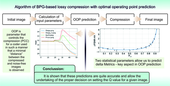
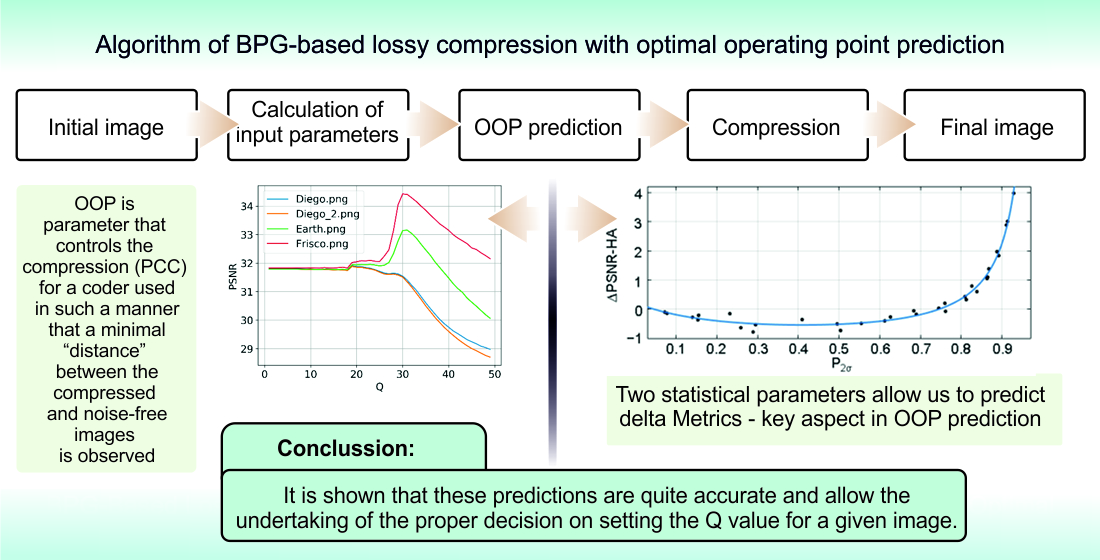
BPG-Based Lossy Compression of Three-Channel Noisy Images with Prediction of Optimal Operation Existence and Its Parameters

Abstract

Nowadays, there is a clear trend toward increasing the number of remote-sensing images acquired and their average size. This leads to the need to compress the images for storage, dissemination, and transfer over communication lines where lossy compression techniques are more popular. The images to be compressed or some of their components are often noisy. They must therefore be compressed taking into account the properties of the noise. Due to the noise filtering effect obtained during lossy compression of noisy images, an optimal operating point (OOP) may exist. The OOP is a parameter that controls the compression for which the quality of the compressed image is closer (closest) to the corresponding noise-free image than the quality of the noisy (original, uncompressed) image according to some quantitative criterion (metric). In practice, it is important to know whether the OOP exists for a given image, because if the OOP exists, it is appropriate to perform the compression in the OOP or at least in its neighborhood. Since the real image is absent in practice, it is impossible to determine a priori whether the OOP exists or not. Here, we focus on three-channel-remote-sensing images and show that it is possible to easily predict the existence of the OOP. Furthermore, it is possible to predict the metric values or their improvements with appropriate accuracy for practical use. The BPG (better portable graphics) encoder is considered a special case of an efficient compression technique. As an initial design step, the case of additive white Gaussian noise with equal variance in the three components is considered. While previous research was mainly focused on predicting the improvement (reduction) of the PSNR and PSNR-HVS-M metrics, here we focus on the modern visual quality metrics, namely PSNR-HA and MDSI. We also discuss what to do if, according to the prediction, an OOP is absent. Examples of lossy compression of noisy three-channel remote sensing images are given. It is also shown that the use of three-dimensional compression provides a compression ratio increase by several times compared with component-wise compression in the OOP.

1. Introduction

Many remote-sensing (RS) systems and complexes are used nowadays, and many projects are in progress. The main reason is that RS systems and complexes can operatively provide valuable data for ecological monitoring, agriculture, forestry, and other fields [1,2,3,4]. An obvious advantage of RS is that it is possible to monitor territories of large areas and estimate and control their parameters in real time. A better spatial resolution and more frequent observation of territories are also positive features of RS that make it attractive and beneficial for modern applications.

Meanwhile, improved spatial resolution, more frequent observations, and the use of more spectral (or polarization) components in multichannel (multispectral, hyperspectral, dual, and full-polarization) RS imaging systems lead to several data processing problems and managing issues [4,5]. In particular, it becomes necessary to compress RS images where, in general, lossless and lossy compression approaches are possible [6,7,8]. An advantage of lossless compression [6,7] is that it does not introduce any distortions into the RS data. However, the compression ratio (CR) attained by lossless compression techniques is often too low and not appropriate. Lossy compression can achieve higher CR values [6,8,9,10,11]. Meanwhile, a higher CR results in the introduction of larger distortions. Therefore, a reasonable compromise needs to be found and proposed [12].

Note that different viewpoints can characterize distortions using different metrics [12,13,14,15]. Whilst metrics that are conventional for image processing are still widely used in remote sensing, such as mean square error (MSE) or peak signal-to-noise ratio (PSNR), other measures of compressed image quality are also employed. They might be related to an end task of RS data processing, for example, the probability of correct classification [13,14,15], which can even be improved by lossy compression under certain conditions [13,14]. The use of visual quality metrics is also becoming popular [16,17]. There are two main reasons for this. First, compressed RS images are often subjected to visual inspection and analysis. Second, the visual quality metric values correlate quite highly with the accuracy of parameter estimation and the probability of correct classification for “heterogeneous” classes such as Urban or Forest, which typically contain textures and abrupt changes. The novelty of this paper is partly related to our decision to focus on the analysis of visual quality metrics such as the Mean Deviation Similarity Index (MDSI) [18] and PSNR-HA [19], which are among the best full-reference visual quality metrics [20] for color and three-channel images. Note that we prefer considering the visual quality metrics with approximately linear behavior and avoid working with the metrics of the SSIM-based family (such as MS-SSIM or color version of FSIM) because of their sufficiently nonlinear properties that create problems in prediction and interpretation of their results.

One further peculiarity of this paper is that we consider three-channel RS images. Multichannel imaging is the primary mode of operation for RS sensors today. The term “multichannel” includes multispectral [1] imaging, joint optical and radar observations [3], dual and full-polarization radar [21,22], and hyperspectral [23] imaging. Three-channel images are the simplest cases of such RS data. The tendencies and observations obtained for these images can be later generalized for images with a larger number of components. It should be noted that multichannel observation opens up new possibilities for remote sensing and/or improves the accuracy of parameter estimation, classification, and object detection. On the one hand, a larger number of RS image components increases the need for more efficient RS data compression. On the other hand, CR in this case can be increased (compared with component-wise compression) using three-dimensional compression of multichannel images that exploits sufficient correlation between component images [7,11,15].

Many papers discuss lossy compression of RS data under the assumption that images are free of noise (see, e.g., ref. [9,10,24,25] and references therein). However, this assumption is not always valid in practice. Let us give some examples of remote sensing when noise is visible in acquired images and can be intensive. A first example is speckle, which is always present in synthetic aperture radar images [21,22]. Another example is components of multispectral and hyperspectral RS data, for which the input PSNR can be of the order 20–30 dB [23]. This can also be the case for so-called night-light images [26], etc. Here, we are not interested in the origin of the noise. We only assume that there are three or more components of multichannel RS data for which noise is quite intensive.

The specific features of lossy compression applied to noisy images were discovered approximately 25 years ago [27,28,29,30]. Two features are the most important. First, a noise-filtering effect occurs due to lossy compression. Second, due to this denoising, an optimal operation point (OOP) can be observed for some images and noise properties. Here, by OOP, we mean a parameter that controls the compression (PCC) for a coder used in such a manner that a minimal “distance” between the compressed and noise-free images is observed. This distance can be characterized in different ways, starting from traditional measures such as mean square error (MSE) and peak signal-to-noise ratio (PSNR), and ending with visual quality metrics such as, e.g., PSNR-HVS-M [31] or FSIM [32]. Note that the OOP corresponds to a minimum value of the similarity measure if it is low for similar images, e.g., MSE or MDSI, and vice versa. Moreover, note that different coders apply different PCCs. For JPEG, the quality factor serves as the PCC [33,34]; wavelet-based coders are often controlled by BPP (bits per pixel) [35]; discrete cosine transform (DCT)-based coders are usually controlled by quantization step (QS) [36]; and for the modern better portable graphics (BPG) coder, a special parameter Q is used as the PCC [37,38].

If an OOP exists for a given image and the coder used, then compression in the OOP can be beneficial for two reasons. First, the compressed image quality is quite high and, depending on the metric used, is better than the quality of the original image (or the image compressed in a lossless manner, or the image compressed with another PCC). Second, the CR observed for an OOP-compressed image is generally sufficiently high. In addition, OOP compression can be beneficial for image classification [39]. On the other hand, if OOP does not exist, a more “conservative” compression is desired [40].

Then, at least two particular tasks have to be solved. First, it is necessary to know how to set the PCC for a given coder applied to a noisy image to compress this image at the OOP if it exists. Second, it is necessary to predict whether or not an OOP exists in order to properly set the PCC in both cases.

Sufficient research has been already performed to answer these questions for single-component images. In the papers [41,42], it was demonstrated that the OOP can be reached iteratively [41] or in a single step [42] for DCT-based coders controlled by QS if noise is additive, white, and Gaussian, and its variance is known a priori. In [43], it was shown that reaching the OOP is possible for the SPIHT coder under the same conditions. The authors of [44,45] proved that the OOP can be reached automatically for DCT-based coders for signal-dependent noise with a priori known characteristics. The case of BPG coder applied to noisy images has been considered in [40,46]. The case of single-component images has been studied in depth there. However, for three-channel images, only preliminary analysis results showing that the OOP can exist were given [40]. Note that the results in [47] show that the OOP is more likely if multichannel noisy images are jointly compressed compared with component-wise compression. The possibility of predicting the existence of the OOP has been demonstrated in [36,40].

Keeping this summary in mind, in this paper, we concentrate on the BPG-based lossy compression of three-channel images corrupted by additive white Gaussian noise (AWGN) supposed to have zero mean and equal variances in all components. We show that, as in [36,40], the presence of the OOP and the compression in this point can be easily predicted prior to compression based on a calculation of statistical parameters previously used in image denoising theory [48,49]. The paper novelty consists of the following. First, we show that 3D compression has clear benefits compared with component-wise compression in the OOP in the sense of having a CR that is several times larger, and better values of PSNR-HA and MDSI. Second, the presented results of our studies allow the choice of the best option among the compression versions 4:4:4, 4:2:2, and 4:2:0, as well as predicting the existence of the OOP for all three of these versions. Third, we give a modified formula for Q_OOP for the 3D case that differs from the one for the single component case. Fourth, the metrics intended for the characterization of quality for three-channel (color) images are considered and it is shown that prediction is possible not only for the metrics of PSNR-like family but for MDSI as well. Finally, our recommendations and conclusions are supported by the results and statistics for more than 30 images.

The structure of the document is as follows. Section 2 describes the image/noise model used and it also presents the metrics considered and explains the basic criteria and dependencies. Section 3 deals with the prediction of the OOP. The methodology for obtaining the dependencies is given and discussed. Decision-making and some practical aspects are considered in Section 4. Results of statistical testing for three versions of 3D compression and component-wise compression for a set of 20 three-channel images not used in training (scatter-plot obtaining and regression) are also presented in section. Finally, the conclusions and directions for future studies are presented.

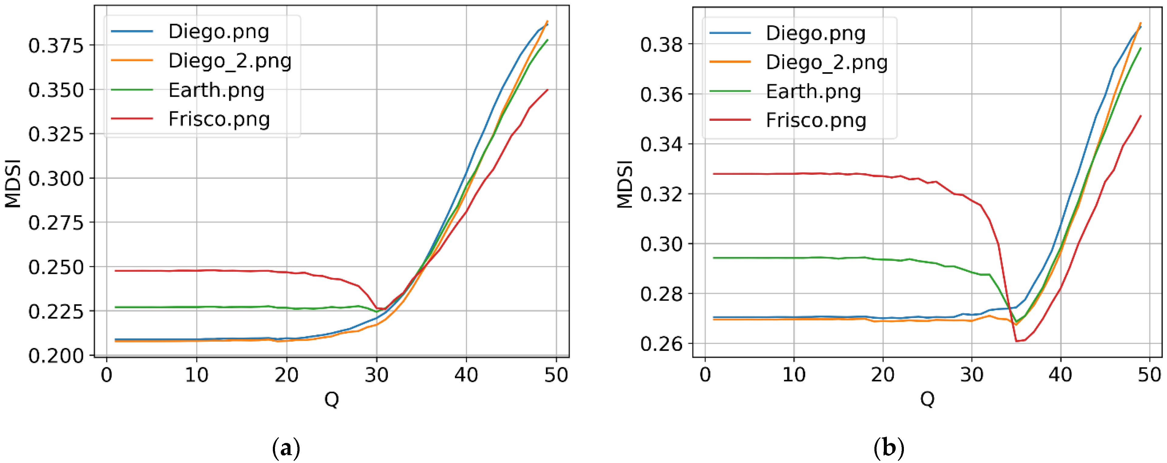
2. Image/Noise Model and Behavior of Compression Efficiency Criteria

In this paper, we consider the AWGN model for all components of three-channel images. This is because of several reasons. First, this is the simplest model often used in the theory and practice of image processing [50,51] and we need a starting point in our research. Second, if noise is not additive (it is signal-dependent), there are the so-called variance-stabilizing transforms that allow the conversion of images corrupted by signal-dependent noise to images corrupted by practically pure additive noise [44,45,52] and this offers favorable conditions for further lossy compression. Note that there are numerous methods for blind estimation of noise characteristics of additive and signal-dependent noise (see [53,54,55] and references therein). This allows the assumption that we know noise variance in component images in advance.

Thus, one has the following model of an observed noisy three-channel image

$$I_{ijk}^n=I_{ijk}^{true}+n_{ijk},$$

where $I_{ijk}^{true}$, $i=1,\dots ,I_{Im},j=1,\dots ,J_{Im},k=1,\dots ,3$ is the true or noise-free image in a k-th component, $n_{ijk}$ denotes AWGN in the $ij$-th pixel of a k-th component, and $I_{Im}$ and $J_{Im}$ define the image size. The noise mean is assumed to be equal to zero whilst the AWGN variance is supposed to be equal to ${\sigma }^2$ in all components and it is assumed to be known in advance. The assumption that noise variance is the same in all components is one more simplification dealing with the possible use of variance-stabilizing transforms.

For the preliminary study, we use four test three-channel images (Figure 1) visualized as color ones from the USC-SIPI image database—Aerials (https://sipi.usc.edu/database/database.php?volume=aerials (accessed on 15 March 2023)). Our goal is to study peculiarities of rate/distortion dependencies for images of different complexities where we consider that the image Frisco (Figure 1a) is of simple structure, the image Earth (Figure 1c) is of middle complexity, and the images Diego and Diego 2 (Figure 1b,d, respectively) are complex ones since they contain many small objects (details) and textures.

A standard way to characterize the quality of the original noisy image is to use

$${PSNR}^n=10{log}_{10}\left(\frac{{255}^2}{{\sigma }^2}\right),$$

(1)

that relates to the case of equal variance values in all components where images in all components are represented as 8-bit two-dimensional (2D) arrays of integers.

In turn, a standard way to obtain and analyze rate/distortion curves is to calculate a metric between the original (in our case, noisy) and compressed images for a set of PCC values. Thus, we have to give brief information concerning the BPG coder. First, we have used the coder realization freely available at http://bellard.org/bpg/ (accessed on 15 March 2023). The reasons for our interest in this coder are explained by its advantages. BPG provides a higher compression rate with the same quality compared with the commonly used analogs (e.g., JPEG).

Second, BPG is supported by the most popular Web browsers. Third, BPG supports the same formats as JPEG, including grayscale, YCbCr 4:2:0, 4:2:2, and 4:4:4. Color spaces such as RGB, YCgCo, and CMYK are supported. We have not found papers and examples dealing with the use of the BPG coder in remote sensing. However, we have found discussions concerning this in https://lwn.net/Articles/625535/ (accessed on 15 March 2023) as well as examples of successful application of the BPG coder in medical image compression [38].

We would like to pay special attention to the formats 4:2:0, 4:2:2, and 4:4:4 where the first and second formats relate to color component subsampling. On the one hand, their use allows to partly solve the near-lossless compression task.

On the other hand, subsampling of color component images leads to introducing additional and specific distortions that have to be studied with application to lossy compression of noisy three-channel images.

Thus, let us look at the dependencies of PSNR_nc on Q where the notation PSNR_nc is calculated between the original and compressed images and Q serves as PCC for the BPG encoder (Q are integers from 1 to 51 where smaller values correspond to a smaller CR).

As is typical for lossy compression, the quality of compressed images becomes worse if the CR increases. This is seen in Figure 2 where we present the plots PSNR_nc(Q) for all three possible formats of noisy image representation (${\sigma }^2=49$). For all formats and for all test images, the considered rate/distortion curves monotonously decrease. However, there are significant differences in their behavior depending on the compressed image format. For the format 4:4:4 (Figure 2a), one can observe three obvious intervals of different behavior. If Q < 7, PSNR_nc(Q) ≈ 53 dB, i.e., losses introduced by compression are negligible and one is unable to notice the differences between the original and the corresponding compressed images. Then, for 7 ≤ Q ≤ Q_upp, there is practically a linear dependence that can be approximated as PSNR_nc(Q) ≈ 60 − Q where Q_upp approximately corresponds to input PSNR defined by (1) (approximately 31.3 dB for the considered case of ${\sigma }^2=49$). For the two aforementioned intervals, the rate/distortion curves for different images practically coincide. For the third interval, Q > Q_upp, the curves continue to decrease although the decrease is slower for the images with simpler structures (Frisco and Earth).

Here, it is worth recalling some properties of the metric PSNR. Although it is not the best metric for characterizing the visual quality of images [56,57], it is possible to state [57] that distortions start to become visible if PSNR is approximately 35 dB. This means that compression with Q ≤ 25 does not lead to visible distortions. For larger Q, distortions are associated both with simultaneous noise suppression and information degradation, and a more careful analysis is needed.

One peculiarity of dependencies PSNR_nc(Q) for the formats 4:2:2 (Figure 2b) and 4:2:0 (Figure 2c) is that they behave individually. They start (Q = 1) from PSNR_nc at approximately 34 dB (Figure 2b) and 32.5 dB (Figure 2c). This means that the images already sufficiently differ from the original ones after subsampling. For Q < 15, the quality of compressed images remains practically the same as for Q = 1. Then, for a larger Q, there is an obvious tendency to have a larger difference between an original and the corresponding compressed images. A comparison of the corresponding curves in Figure 2b,c shows that PSNR_nc values for the format 4:2:2 are slightly larger for a small Q.

The dependencies PSNR_nc(Q) do not show what happens to the noise if lossy compression is applied to noisy images. Because of this, dependencies PSNR_tc(Q) and Metr_tc(Q) are often considered where subscript tc indicates that a full-reference metric (Metr) is calculated between the compressed and the corresponding true (noise-free) images. Certainly, this is impossible in practice when one has a noisy image to be compressed and any noise-free image is absent. However, this is possible in the analysis of simulated data when one has a noise-free image, adds noise to it, and then applies compression with several PCC values [36,40,41,42,43,44,45,46]. Such analysis is beneficial since it allows an understanding of how the properties of compressed images change with changes to the PCC values.

As an example of such dependencies, Figure 3 presents the plots PSNR_tc(Q) for all three considered formats. As it is seen, the plots for simple and middle complexity images Frisco and Earth have obvious maxima (optimal operation points) observed for Q_OOP = 30. In turn, the plots for the complex structure images Diego and Diego 2 either do not have obvious maxima or are monotonously decreasing. This example shows that it is worth compressing simple structure images in OOP whilst for complex structure images it is not clear what to do. At the moment, it seems that it is worth using a Q_rec smaller than the Q_OOP to avoid considerable distortions. The examples provided also explain why it is reasonable to predict if OOP exists for a given image and noise variance.

Although dependencies for the same image but different formats seem similar, there are some differences. The main difference is that PSNR_tc in the OOP for simple structure images is usually the largest for the format 4:4:4 (Figure 3a). Moreover, whilst PSNR_tc is the same for all test images for the format 4:4:4 for small Q, it is different for various images for the formats 4:2:2 and 4:2:0 (Figure 3b,c).

For the considered case of ${\sigma }^2=49$, we have Q_OOP = 30. A thorough analysis has been carried out in [58] for the metrics PSNR-HVS-M [57] and MSSIM [59] for ${\sigma }^2=100,$ and it has been demonstrated that the OOP (if it exists) takes place at Q_OOP = 32 or 33. Additional analysis has been carried out in our paper [60] for the visual quality metrics PSNR-HA [20] and MDSI [19] for ${\sigma }^2=100$. It has been shown again that there are images for which the OOP exists (according to the aforementioned metrics) and this occurred at Q_OOP = 33. Figure 4 shows the plots for the metric MDSI [19] for two other values of noise variance—${\sigma }^2=64$ and ${\sigma }^2=196$ (here it is worth recalling that for the metric MDSI, in contrast to other visual quality metrics, smaller values correspond to better visual quality). Analysis shows that obvious local minima are observed for simple structure images. For ${\sigma }^2=196$, a “non-obvious” minimum exists even for the complex structure image Diego 2. For ${\sigma }^2=64$, one has Q_OOP = 31 (Figure 4a) whilst, for ${\sigma }^2=196$, the OOP is observed at Q_OOP = 36.

The presented results, as well as analysis of other data obtained during our experiments, show several important tendencies. First, for a given noise variance, Q_OOP (if OOP exists) is practically the same for different metrics and different images. The same was observed for lossy compression of grayscale images corrupted by AWGN [40]. However, for three-channel images, Q_OOP is slightly smaller than Q_OOP for grayscale (single-channel) images for the same variance of AWGN. In [40], it has been found for grayscale images that

$$Q_{OOP}\approx 14.9+20{log}_{10}\left(\sigma \right)$$

(2)

Meanwhile, in [60], for three-channel data, it is recommended to determine Q for the OOP as (see the data in Figure 3 and Figure 4 for confirmation)

$$Q_{OOP}\approx 12.9+20{log}_{10}\left(\sigma \right).$$

(3)

The reason for this is the following: in the case of three-channel images, they are first converted to YCbCr color format and then the BPG compression is applied component-wise (decompression performs in inverse order). Such a conversion (https://en.wikipedia.org/wiki/YCbCr (accessed on 15 March 2023)) changes noise variance and reduces the range of image data representation. In particular, noise variances in component images become ${\sigma }_Y^2\approx 0.45{\sigma }^2$, ${\sigma }_{Cb}^2\approx 0.39{\sigma }^2$, and ${\sigma }_{Cr}^2\approx 0.43{\sigma }^2,$ i.e., smaller than in RGB components. Thus, optimal Q should be smaller as well.

Second, due to the Formula (3) introduced above, it becomes possible to determine Q_OOP (here it does not matter whether OOP exists or not). Then, our task is to obtain some information concerning the considered quality metric for Q = Q_OOP that will allow deciding if OOP exists or not, and what Q to set.

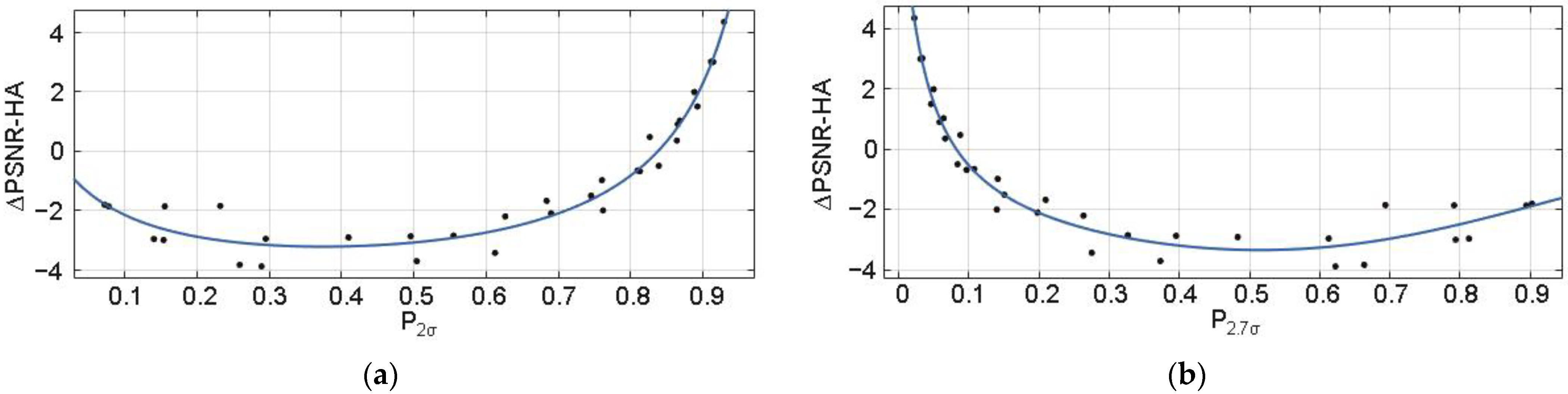
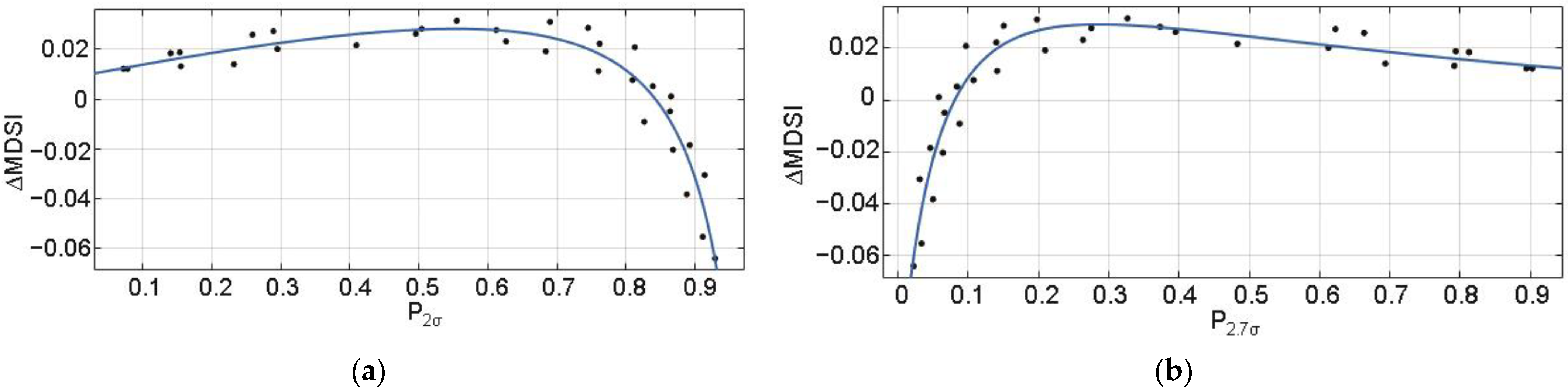
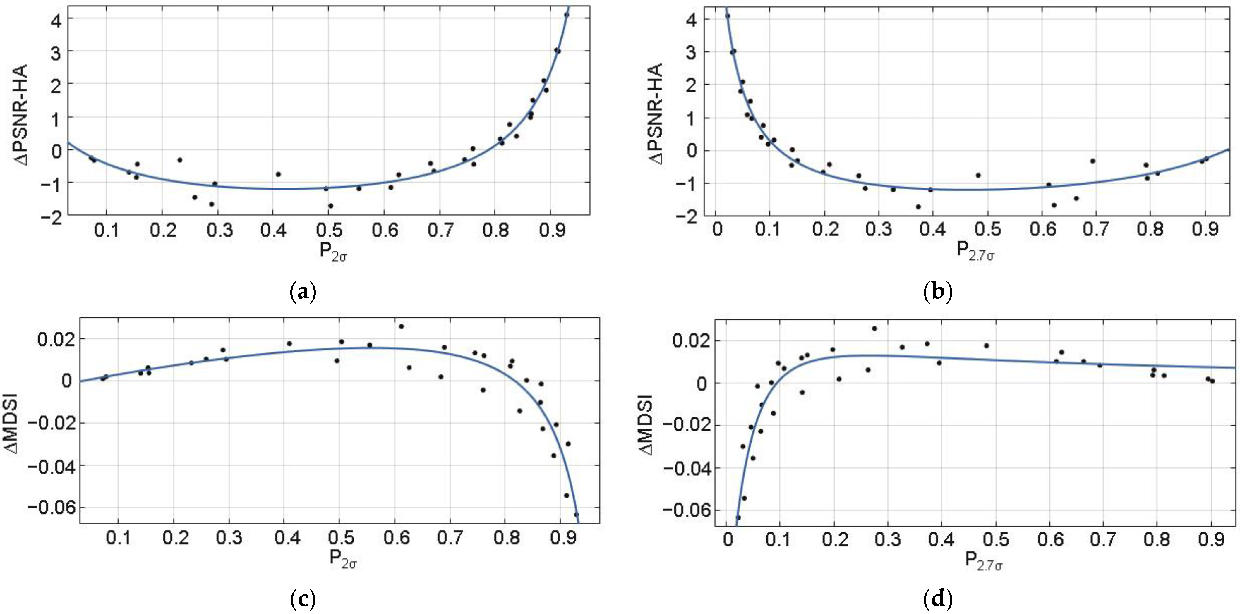
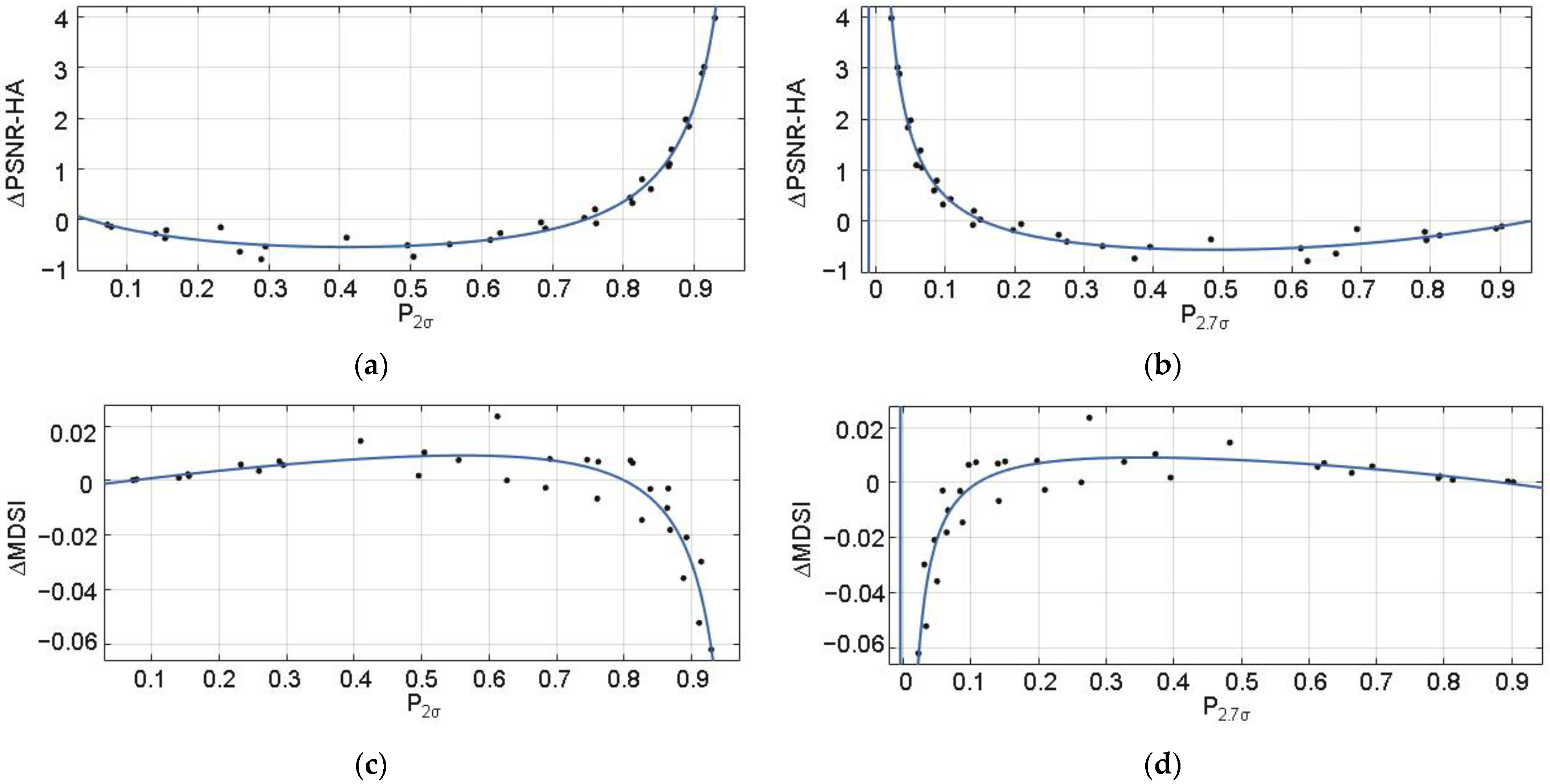
3. Prediction of OOP Existence and Parameters in It

We state that the existence of the OOP can be predicted. Our confidence is based on earlier-obtained results and experience [36,40]. The main difference between the results given below compared with the results in [36,40] is that we consider three-channel images and the visual quality metrics PSNR-HA [20] and MDSI [19], which were not analyzed with application to lossy image compression earlier.

Recall here some basic ideas of the papers [36,40]. First, it is assumed that it is possible to somehow predict or estimate the difference ${∆Metr=Metr}_{}^{tc}\left(Q_{OOP}\right)-{Metr}_{}^{tc}(Q=1)$ where ${Metr}_{}^{tc}\left(Q_{OOP}\right)$ is the considered metric in Q_OOP calculated according to (3). Suppose that if a given metric is larger for better quality (as PSNR-HA in our case), then $∆Metr>0$ is the evidence in favor of the existence of the OOP. Similarly, if a given metric is smaller for better quality (as MDSI in our case), then the OOP exists if $∆Metr<0$. Thus, in fact, we should know the sign of $∆Metr$ to understand if the OOP exists or not.

Second, the prediction is based on a simple procedure. Two statistical parameters, $P_{2\sigma }^{}$ and $P_{2.7\sigma }^{}$, have been used in prediction [36,40]. They are both calculated in a limited set of M 8 × 8 pixel blocks in the DCT domain. In further detail, $P_{2\sigma }^{}$ is determined as

$$\begin{gathered} P_{2\sigma }^{}=\sum _{m=1}^M\frac{P_{2\sigma }^{}\left(m\right)}{M}, P_{2\sigma }^{}\left(m\right)=({\sum }_{k=0}^7{\sum }_{l=0}^7\delta (k,l,m))/64, \\ \delta \left(k,l,m\right)=1,if\left|D(k,l,m)\right|<2\sigma \\ 0 \mathrm{otherwise}, \end{gathered}$$

(4)

where $D(k,l,m)$ is the kl-th DCT coefficient for the m-th block. Thus, $P_{2\sigma }^{}$ is the probability that modulus values of DCT coefficients are smaller than 2σ. $P_{2.7\sigma }^{}$ is determined as

$$\begin{gathered} P_{2.7\sigma }^{}=\sum _{m=1}^M\frac{P_{2.7\sigma }^{}\left(m\right)}{M}, P_{2.7\sigma }^{}\left(m\right)=(({\sum }_{k=0}^7{\sum }_{l=0}^7\delta (k,l,m))-1)/63, \\ \delta \left(k,l,m\right)=1,if\left|D(k,l,m)\right|>2.7\sigma \\ 0 \mathrm{otherwise}. \end{gathered}$$

(5)

The Formulas (4) and (5) correspond to the grayscale image case. For the considered three-channel case, probabilities $P_{2\sigma }^{}$ and $P_{2.7\sigma }^{}$ have been separately estimated for the original three (R, G, and B) components and then averaged.

Third, it has been assumed that $∆PSNR-HA$ or $∆MDSI$, i.e., predictor outputs, are strictly connected with input parameters, $P_{2\sigma }^{}$ or $P_{2.7\sigma }^{}$. If such an assumption is valid, then, for a given noisy image (with a known noise standard deviation σ) to be compressed, one calculates $P_{2\sigma }^{}$ or $P_{2.7\sigma }^{}$ and, using the a priori known dependency (function), predicts $∆PSNR-HA$ or $∆MDSI$ or another reliable metric.

Questions that naturally arise are: What is the dependence between input and output parameters? How can it be obtained, and how strict is it? The papers [36,40] already provide possible answers and solutions. Regression using scatter-plots allows the finding of dependencies between output and input parameters whilst parameters characterizing curve fitting as goodness-of-the-fit R², adjusted R², or root mean square error (RMSE) [61] serve as standard indicators of dependency strictness.

This general information requires examples and additional explanations. Let us start by establishing a dependency between $∆PSNR-HA$ and $P_{2\sigma }^{}$ or $P_{2.7\sigma }^{}$ for the format 4:4:4. The scatter-plots are obtained once and in advance (meaning that this work is done off-line and the dependency between output and input parameters is available at the time that the prediction has to be carried out for a given image). The scatterplots are represented in Figure 5. Each point of the scatterplot corresponds to one test image corrupted by AWGN with a given noise standard deviation. Then, the input parameter is estimated and the image is compressed using Q_OOP defined by (3). After decompression, ∆Metr is calculated. In all of the scatterplots, the vertical axis corresponds to the output parameter and the horizontal axis relates to the input parameter. Test images of different complexity are used, and the noise variance varies from 0.25 to 400.

Before analyzing the data in Figure 5, one must know the following. Small $P_{2\sigma }^{}$ and large $P_{2.7\sigma }^{}$ correspond to complex structure images and/or small variance values. PSNR-HA is expressed in dB and its variation by 0.5–1 dB can be observed by visual inspection.

Analysis of the scatterplots in Figure 5 allows the making of the main conclusion—scatterplot points are placed in a compact manner and a good curve fitting is possible. Thus, an accurate prediction is possible for both input parameters (quantitative data are given below). There are situations when $∆PSNR-HA$ is negative and its values are approximately −3 dB. This mostly happens for complex structure images corrupted by AWGN with a variance smaller than 10. Meanwhile, this also happens for the test images Diego and Diego 2 for ${\sigma }^2=25$. There are also images and noise variance values when $∆PSNR-HA$ is negative and its values are approximately −1 dB. One example is the test image Diego corrupted by AWGN with ${\sigma }^2=49$ (Figure 3a). Then, it is reasonable to compress such images with $Q<Q_{OOP}$, e.g., Q = 25 when the introduced distortions are invisible (Figure 2a). There are also images and noise variance values for which $∆PSNR-HA$ is positive. This happens with a high probability if $P_{2\sigma }^{}>0.84$ (Figure 5a) or $P_{2.7\sigma }^{}<0.08$ (Figure 5b). Positive values of $∆PSNR-HA$ mainly take place for simple structure images corrupted by quite intensive noise (one example is the test image Frisco corrupted by AWGN with ${\sigma }^2=49$ (Figure 3a). Then, compression at the OOP is expedient.

Let us analyze the data for the metric $∆MDSI$. The scatter-plots and the fitted curves are given in Figure 6. Note here that the MDSI varies in the limits from 0 to approximately 0.6 where a difference of approximately 0.02 can be noticed. Again, the scatter-plot points are placed in a compact manner and a good fitting is possible.

Conclusions that can be drawn from the analysis of data in Figure 6 are as follows. There are positive values of $∆MDSI$ that correspond to $P_{2\sigma }^{}<0.85$ (Figure 6a) or to $P_{2.7\sigma }^{}>0.08).$ Then, compression has to be carried out “with care”, i.e., using $Q<Q_{OOP}$, e.g., Q_OOP = 25 (an example of such a situation is the test image Diego corrupted by AWGN with ${\sigma }^2=64$, Figure 4a). In the opposite situations, i.e., for $P_{2\sigma }^{}\ge 0.85$ (Figure 6a) or $P_{2.7\sigma }^{}\le 0.08$, the OOPs are observed with high probability and it is worth compressing the corresponding images at the OOP.

Let us briefly consider the data obtained for other formats. The scatterplots for the format 4:2:2 are presented in Figure 7. The scatterplot in Figure 7a is very similar to the one in Figure 5a, whilst the scatterplot in Figure 7b is similar to that one in Figure 5b. Thus, the conclusions are practically the same. According to the metric ${∆PSNR-HA}_{}^{}$, the OOP exists if $P_{2\sigma }^{}\ge 0.85$ (Figure 7a) or $P_{2.7\sigma }^{}\le 0.1$ (Figure 7b). The scatter-plot in Figure 7c is similar to the one in Figure 6a, whilst the scatter-plot in Figure 7d is analogous to the one in Figure 6b. According to the metric $∆MDSI$, the conclusions are practically the same as according to $∆PSNR-HA$: the OOP exists if $P_{2\sigma }^{}\ge 0.82$ (Figure 7c) or $P_{2.7\sigma }^{}\le 0.1$ (Figure 7d). Thus, the results for two different visual metrics are in quite strong agreement.

The scatterplots for the format 4:2:0 are given in Figure 8. The scatterplot in Figure 8a is quite similar to the ones in Figure 5a and Figure 7a; the scatterplot in Figure 8b is quite similar to those in Figure 5b and Figure 7b. Th analysis of the data in Figure 8a,b leads to practically the same conclusions as earlier. According to the metric ${∆PSNR-HA}_{}^{}$, the OOP exists if $P_{2\sigma }^{}\ge 0.76$ (Figure 8a) or $P_{2.7\sigma }^{}\le 0.14$ (Figure 8b). These recommendations slightly differ from previous ones obtained for the formats 4:4:4 and 4:2:2.

The scatter-plot in Figure 8c is similar to those in Figure 6a and Figure 7c, whilst the scatter-plot in Figure 8d is analogous to the ones in Figure 6b and Figure 7d. The analysis of the metric $∆MDSI$ allows the conclusion that the OOP exists if $P_{2\sigma }^{}\ge 0.81$ (Figure 8c) or $P_{2.7\sigma }^{}\le 0.11$ (Figure 8d). These results and conclusions are in good agreement with the above recommendations for the formats 4:4:4 and 4:2:2.

Thus, the results for different formats differ somewhat but the general tendencies are the same. The values of Q_OOP for all three formats practically coincide, but the quality metric values in the OOP slightly differ. Because of this, additional comparison and analysis are required. This will be undertaken in the next Section; additionally, some comparison results are given in [60] where it is shown that each format has its advantages and drawbacks.

Here, we would like to pay attention to curve fitting. In general, it is more of an engineering task than a scientific task. Meanwhile, while solving the curve-fitting task for our application, we have taken into account the following.

First, according to visual inspection of the scatter-plot properties, the fitted curves have to be smooth enough. Second, there are special tools available that are designed for curve fitting (regression); we have used a MATLAB Curve Fitting Tool. Third, relying on previous experience [40], we have employed rational functions (the fitted curves in Figure 5, Figure 6, Figure 7 and Figure 8 are obtained using such functions). The function parameters and the fitting criteria are given in

Table 1. Parameters of the fitted curves.

Dependence	Expression	Parameters	R2	Adjusted R2	RMSE
$∆PSNR-HA$ on $P_{2\sigma }^{}$ (4:4:4)	f(x) = (p1 × x2 + p2 × x + p3)/(x3 + q1 × x2 + q2 × x + q3)	p1 = 1.195 × 105 p2 = −1.003 × 105 p3 = 147.4 q1 = −1.92 × 104 q2 = 1.778 × 104 q3 = 2454	0.9530	0.944	0.5143
$∆PSNR-HA$ on $P_{2.7\sigma }^{}$ (4:4:4)	f(x) = (p1 × x2 + p2 × x + p3)/(x3 + q1 × x2 + q2 × x + q3)	p1 = 3.114 p2 = −4.159 p3 = 0.3203 q1 = −1.482 q2 = 1.015 q3 = 0.03138	0.9539	0.945	0.5094
$∆MDSI$ on $P_{2\sigma }^{}$ (4:4:4)	f(x) = (p1 × x2 + p2 × x + p3)/(x3 + q1 × x2 + q2 × x + q3)	p1 = −36.59 p2 = 25.2 p3 = 4.732 q1 = −59.71 q2 = −478.2 q3 = 547.8	0.9154	0.8991	0.007974
$∆MDSI$ on $P_{2.7\sigma }^{}$ (4:4:4)	f(x) = (p1 × x2 + p2 × x + p3)/(x3 + q1 × x2 + q2 × x + q3)	p1 = −61.94 p2 = 110.5 p3 = −8.54 q1 = 2341 q2 = 1243 q3 = 71.58	0.9036	0.885	0.008512
$∆PSNR-HA$ on $P_{2\sigma }^{}$ (4:2:2)	f(x) = (p1 × x2 + p2 × x + p3)/(x3 + q1 × x2 + q2 × x + q3)	p1 = 4.964 × 104 p2 = −4.162 × 104 p3 = 1942 q1 = −1.602 × 104 q2 = 1.342 × 104 q3 = 2861	0.965	0.9582	0.2938
$∆PSNR-HA$ on $P_{2.7\sigma }^{}$ (4:2:2)	f(x) = (p1 × x2 + p2 × x + p3)/(x3 + q1 × x2 + q2 × x + q3)	p1 = −5.772 × 104 p2 = 6.093 × 104 p3 = −6402 q1 = 2.003 × 104 q2 = −2.481 × 104 q3 = −717.6	0.9623	0.9551	0.3048
$∆MDSI$ on $P_{2\sigma }^{}$ (4:2:2)	f(x) = (p1 × x2 + p2 × x + p3)/(x3 + q1 × x2 + q2 × x + q3)	p1 = −25.17 p2 = 21.54 p3 = −0.8092 q1 = −152 q2 = −256 q3 = 408.8	0.8778	0.8543	0.007885
$∆MDSI$ on $P_{2.7\sigma }^{}$ (4:2:2)	f(x) = (p1 × x + p2)/(x2 + q1 × x + q2)	p1 = 0.008652 p2 = −0.0008153 q1 = 0.1452 q2 = 0.00661	0.853	0.8372	0.008334
$∆PSNR-HA$ on $P_{2\sigma }^{}$ (4:2:0)	f(x) = (p1 × x2 + p2 × x + p3)/(x3 + q1 × x2 + q2 × x + q3)	p1 = 6922 p2 = −5483 p3 = 243.9 q1 = −4101 q2 = 3003 q3 = 1025	0.9869	0.9843	0.1482
$∆PSNR-HA$ on $P_{2.7\sigma }^{}$ (4:2:0)	f(x) = (p1 × x2 + p2 × x + p3)/(x3 + q1 × x2 + q2 × x + q3)	p1 = 2.433 p2 = −2.668 p3 = 0.3562 q1 = −2.571 q2 = 2.324 q3 = 0.02283	0.9844	0.9814	0.1615
$∆MDSI$ on $P_{2\sigma }^{}$ (4:2:0)	f(x) = (p1 × x2 + p2 × x + p3)/(x3 + q1 × x2 + q2 × x + q3)	p1 = −12.84 p2 = 11.17 p3 = −0.7154 q1 = −86.94 q2 = −255.8 q3 = 334.8	0.8558	0.8281	0.007658
$∆MDSI$ on $P_{2.7\sigma }^{}$ (4:2:0)	f(x) = (p1 × x2 + p2 × x + p3)/(x3 + q1 × x2 + q2 × x + q3)	p1 = −0.4441 p2 = 0.4425 p3 = −0.04341 q1 = −10.63 q2 = 21.37 q3 = 0.05467	0.8431	0.813	0.007988

.

Analysis of the data given in Table 1 shows the following. First, for the metric $∆PSNR-HA$, the fitting is very good for all formats. The values of R² are approximately 0.97 (from 0.95 till 0.99), and RMSE is approximately or less than 0.5 dB. These are appropriate pre-conditions for accurate prediction. Second, fitting for the metric $∆MDSI$ is characterized by an R² of approximately 0.9 for the format 4:4:4 and approximately 0.83 for the two other formats. Such accuracy is acceptable in practice as well. Third, the input parameter to be used makes almost no difference since the values R² and RMSE (for the same format and predicted metric) are practically the same.

4. Decision Undertaking and Other Practical Aspects

4.1. Prediction Verification and Additional Accuracy Analysis

First of all, we have to be sure that the proposed approach to prediction performs well enough. For this purpose, let us select the three-channel images that have not been exploited in the obtaining of the scatter-plots. Such images are represented in Figure 9, where there are four RS images of different complexity. Using the obtained fitted curves (regressions), we have carried out an experiment for AWGN with a variance equal to 100. $∆PSNR-HA$ and $∆MDSI$ values have been predicted using both considered input parameters and calculated for images compressed at the OOP. The obtained data are collected in

Table 2. Predicted and true parameters for verification images compressed with Q_OOP.

Image	Format	Input Parameter	Predicted $∆\mathit{P}\mathit{S}\mathit{N}\mathit{R}-\mathit{H}\mathit{A}$	Calculated $∆\mathit{P}\mathit{S}\mathit{N}\mathit{R}-\mathit{H}\mathit{A}$	Predicted $∆\mathit{M}\mathit{D}\mathit{S}\mathit{I}$	Calculated $∆\mathit{M}\mathit{D}\mathit{S}\mathit{I}$
Woodland Hills	4:4:4	$P_{2\sigma }^{}$	−1.7	−1.8	0.021	0.033
		$P_{2.7\sigma }^{}$	−1.64		0.023
Point Loma	4:4:4	$P_{2\sigma }^{}$	2.2	1.8	−0.031	−0.018
		$P_{2.7\sigma }^{}$	2.52		−0.037
Foster City	4:4:4	$P_{2\sigma }^{}$	0.53	0.97	−0.006	−0.024
		$P_{2.7\sigma }^{}$	0.53		−0.008
Shelter Island	4:4:4	$P_{2\sigma }^{}$	−0.29	−0.74	0.005	0.008
		$P_{2.7\sigma }^{}$	−0.29		0.005
Woodland Hills	4:2:2	$P_{2\sigma }^{}$	−0.42	−0.52	0.01	0.019
		$P_{2.7\sigma }^{}$	−0.43		0.01
Point Loma	4:2:2	$P_{2\sigma }^{}$	2.31	2.16	−0.031	−0.019
		$P_{2.7\sigma }^{}$	2.6		−0.037
Foster City	4:2:2	$P_{2\sigma }^{}$	1.04	1.6	−0.011	−0.023
		$P_{2.7\sigma }^{}$	1.08		−0.011
Shelter Island	4:2:2	$P_{2\sigma }^{}$	0.48	0.18	−0.002	0.01
		$P_{2.7\sigma }^{}$	0.48		−0.001
Woodland Hills	4:2:0	$P_{2\sigma }^{}$	−0.02	−0.12	0.005	0.012
		$P_{2.7\sigma }^{}$	−0.02		0.005
Point Loma	4:2:0	$P_{2\sigma }^{}$	2.18	2.09	−0.029	−0.016
		$P_{2.7\sigma }^{}$	2.45		−0.033
Foster City	4:2:0	$P_{2\sigma }^{}$	1.06	1.57	−0.011	−0.021
		$P_{2.7\sigma }^{}$	1.09		−0.01
Shelter Islands	4:2:0	$P_{2\sigma }^{}$	0.62	0.47	−0.004	0.007
		$P_{2.7\sigma }^{}$	0.62		−0.004

.

Analysis of the data shows the following: (1) predictions based on both considered input parameters are very close for both of the predicted metrics; (2) predictions are quite close to the obtained (calculated) values of the studied metrics; (3) predictions show that the OOP exists for the test image Point Loma according to both metrics for all three formats and the image Foster City, also according to both metrics and for all three formats; whereas the OOP does not exist for the image Woodland Hills according to both metrics for all three formats; and (4) the situation is borderline for the image Shelter Islands—the OOP does not exist for the format 4:4:4, but it does exist according to $∆PSNR-HA$ for the formats 4:2:2 and 4:2:0, although the values of the metric $∆MDSI$ are very close to zero.

4.2. Visual Analysis and Decision Undertaking

Let us give some examples of noisy image compression. Figure 10a presents the test image Frisco corrupted by AWGN with a variance equal to 100. Noise is seen, especially in homogeneous image regions. Images compressed in OOP for the original formats 4:4:4, 4:2:2, and 4:2:0 are shown in Figure 10b–d, respectively. It is seen that noise is sufficiently suppressed whilst useful information (edges, textures, small-sized objects) is preserved well for all three formats. It is difficult to detect a considerable difference in the visual quality of images in Figure 10b–d. The main conclusion is that compression at the OOP is reasonable. The question of which format to use will be discussed later.

Let us analyze the results for the complex-structure image Woodland Hills. The original (noisy) image for the same noise variance (100) is shown in Figure 11a. Noise can be noticed in some quasi-homogeneous image regions whilst it is masked in image areas containing texture and fine details.

The image in Figure 11b shows the image Woodland Hills compressed with Q = 33 (i.e., with Q = Q_OOP) for the format 4:4:4. It is possible to see that there is some reduction of the noise, although information degradation (smoothing) is observed as well. Figure 11c,d present the images compressed with Q = 31 (Q_OOP − 2) and Q = 29 (Q_OOP − 4), respectively (the same format). If Q reduces, noise suppression efficiency becomes worse and the CR decreases, but the edge/texture/detail preservation improves. Thus, a reasonable compromise could be to set Q as

Q_rec ≈ Q_OOP − 3

(6)

Summarizing the results presented above, it is possible to propose the following practical algorithm (which is quite similar to that one proposed in [40]):

(1)

If $∆PSNR-HA>1 \mathrm{dB}$, the OOP exists with high probability; then use Q_OOP (3);

(2)

If $-1 \mathrm{dB}\le ∆PSNR-HA\le 1 \mathrm{dB}$, consider that the OOP might exist and use Q = Q_OOP − 1, this allows avoiding image over-smoothing;

(3)

If $∆PSNR-HA$ ≤ −1 dB, use max{Q = Q_OOP − 3, 25} to have invisible distortions, or, at least, distortions that are not annoying (note that in [40] it was recommended to use Q = 29 for analogous case).

4.3. Comparison of Image Compression for Different Formats

Let us first give one example of compressing noisy images for different formats as well as for component-wise and 3D approaches.

Table 3. Data for comparison of compression variants’ performance characteristics.

Q	Format	PSNRtc	PSNR-HAtc	MDSItc	CR
33	4:4:4	32.08	35.01	0.239	33.05
	4:2:2	31.41	34.19	0.239	42.15
	4:2:0	31.05	33.63	0.240	46.29
	Component-wise	29.21	33.46	0.260	7.25
35	4:4:4	31.55	34.23	0.249	51.49
	4:2:2	30.83	33.27	0.249	62.20
	4:2:0	30.51	32.74	0.249	66.76
	Component-wise	31.37	34.62	0.238	15.78

gives the main characteristics of the compressed images for two values of Q: Q = 33 that corresponds to the OOP for the 3D compression (with the conversion from RGB to YCbCr) for the formats 4:4:4, 4:2:2, and 4:2:0; and Q = 35, which corresponds to the OOP for the component-wise compression. The data are obtained for the image Frisco and AWGN variance equal to 100.

Their analysis shows the following. First, the format 4:4:4 provides slightly better quality of compressed images for Q = Q_OOP = 33 and Q = 35 compared with the formats 4:2:2 and 4:2:0. Meanwhile, the format 4:2:0 is characterized by the largest CR (additional data supporting the same tendencies can be found in [60]). Thus, the decision of choosing the best format depends on the priority of the requirements. Second, the component-wise compression at the OOP (Q = 35) provides approximately the same image quality as 3D compression for the formats 4:2:2 and 4:2:0 in OOP (Q = 33), but the CR for the 3D compression is 2–3 times larger. This is an obvious advantage of 3D compression that results from data decorrelation by their conversion from RGB to YCbCr.

Because one example is unable to prove the tendency, we have carried out additional experiments for 20 three-channel images of different complexities (see examples of beach area in Figure 12) used by the authors of [62].

Noise has been artificially added; its variance was equal to 100 in all components. After this, similarly to the data in Table 3, we have determined the PSNR_tc, PSNR-HA_tc, and MDSI_tc for each version of compression for two values of Q—33 and 35. The difference is that we present not all 20 values of PSNR_tc for each image and so on, but mean, minimal, and maximal values determined for the set of twenty test images.

Table 4. Statistical data for comparison of compression variants’ performance characteristics (PSNR_tc).

Q	Format	Mean PSNRtc	Minimal PSNRtc	Maximal PSNRtc
33	4:4:4	35.43	31.94	41.27
	4:2:2	35.25	31.83	41.01
	4:2:0	35.21	31.86	41.01
	Component-wise	29.34	28.52	30.16
35	4:4:4	34.90	31.15	40.99
	4:2:2	34.66	31.08	40.52
	4:2:0	34.65	31.02	40.60
	Component-wise	32.61	29.57	36.68

presents the results for the metric PSNR_tc. The best characteristics (maximal values of mean, minimal and maximal PSNR_tc) are observed for the format 4:4:4 for Q_OOP = 33. They are slightly better than for the formats 4:2:2 and 4:2:0. Meanwhile, these results are also considerably better than for component-wise compression with Q_OOP = 35 (recall that the Q_OOP are different for 3D and component-wise compression). Note that PSNR_tc for Q_OOP vary in wide limits (up to 10 dB) showing the necessity of compressing noisy images with the same intensity of the noise adaptively depending on their complexity.

The results for the metric PSNR-HA_tc are given in

Table 5. Statistical data for comparison of compression variants’ performance characteristics (PSNR-HA_tc).

Q	Format	Mean PSNR-HAtc	Minimal PSNR-HAtc	Maximal PSNR-HAtc
33	4:4:4	36.75	34.70	41.35
	4:2:2	36.59	34.64	41.17
	4:2:0	36.60	34.70	41.17
	Component-wise	34.13	33.48	35.05
35	4:4:4	36.03	33.81	40.78
	4:2:2	35.86	33.76	40.81
	4:2:0	35.85	33.72	40.64
	Component-wise	35.48	33.81	38.71

. Again, the best characteristics (maximal values of mean, minimal and maximal PSNR-HA_tc) are observed for the format 4:4:4 for Q_OOP = 33. The metric values are only slightly better than for the other two formats. The mean results are considerably (by more than 1 dB) better than for component-wise compression with Q_OOP = 35. PSNR_tc for Q_OOP for 3D compression vary in wide limits (up to 7 dB) depending on image complexity.

Let us now proceed with the analysis for the metric MDSI_tc. The obtained data are shown in

Table 6. Statistical data for comparison of compression variants’ performance characteristics (MDSI_tc).

Q	Format	Mean MDSItc	Minimal MDSItc	Maximal MDSItc
33	4:4:4	0.290	0.246	0.320
	4:2:2	0.290	0.246	0.321
	4:2:0	0.290	0.247	0.321
	Component-wise	0.360	0.337	0.381
35	4:4:4	0.299	0.252	0.333
	4:2:2	0.299	0.252	0.332
	4:2:0	0.299	0.253	0.332
	Component-wise	0.303	0.269	0.325

(recall that for this metric, smaller values correspond to better quality). According to the mean values of this metric, there is practically no difference between the formats for both of the considered values of Q. Meanwhile, all three 3D versions of compression with Q_OOP = 33 outperform the component-wise compression with Q_OOP = 35.

Finally, let us examine the data for the CR. They are presented in

Table 7. Statistical data for comparison of compression variants’ performance characteristics (CR).

Q	Format	Mean CR	Minimal CR	Maximal CR
33	4:4:4	106.1	25.5	382.3
	4:2:2	114.9	25.8	422.5
	4:2:0	115.8	25.9	410.7
	Component-wise	7.9	5.8	10.4
35	4:4:4	176.3	35.7	683.0
	4:2:2	185.2	36.0	729.2
	4:2:0	189.9	36.2	756.1
	Component-wise	14.3	5.59	33.3

. As one can see, the mean CR values for the format 4:4:4 are approximately 8% smaller than for two other formats. While the minimal values observed for complex structure images are practically the same, the maximal CR values differ sufficiently. The main point is that for 3D compression with Q_OOP = 35, the CR values are several (4–12) times larger than for component-wise compression with Q_OOP = 35. This is the main advantage of 3D compression where the format 4:2:0 is preferable.

It is also seen that for 3D compression formats, one can use Q = Q_OOP + 1 or Q = Q_OOP + 2. Then, image quality is only slightly worse but the CR can be increased considerably. This is reasonable if providing a larger CR is of prime importance.

We have also analyzed the case of noise variance equal to 25, i.e., if noise is practically not seen. All of the conclusions are the same as for the case of noise variance equal to 100 studied above. There are only two differences. First, the OOP takes place sufficiently more rarely. Second, the CR values are smaller. The mean CR is approximately 50 for 3D formats and approximately 14 for component-wise compression (for the corresponding OOP values).

Additionally, the accuracy of the prediction has been checked for twenty new images not used to obtain the scatter-plots and curve fitting. The obtained values of RMSE are from 1 to 1.6 for the metric PSNR-HA (the smallest RMSE is observed for the 4:2:0 format) and approximately 0.02 for the metric MDSI. These values are larger than the corresponding RMSE for fitting, but they can be considered appropriate for practice.

4.4. Discussion of Practical Aspects

Several important practical aspects deal with computational efficiency, the selection of compression parameters, the influence of different degrading factors, etc.

Concerning computational efficiency, it is worth mentioning the following. First, compression (and decompression) can be parallelized for both the component-wise and 3D compression. In the former case, the components R, G, and B are processed separately and this can be done in parallel. In the latter case, the components Y, Cb, and Cr are processed separately and their parallel processing is also possible (conversion from RGB to YCbCr forward and backward does not take a lot of time). Second, prediction is easy and fast. DCT in 8 × 8 blocks is a standard operation in digital image processing [63] and it can be easily implemented in software or hardware. Moreover, a limited number of blocks (500 or 1000) is needed to accurately estimate an input parameter used. Because of this, the metric prediction and decision undertaking on the Q setting can be done much faster than compression itself. This is a good pre-condition for making the procedure of lossy compression of images corrupted by AWGN fully automatic. Noise variance is known in advance or can be estimated by blind methods [53,54,55,64], then Q_OOP is determined by (3), input and output parameters are determined and, after that, a decision is undertaken concerning what Q to set for the final compression. Even if the noise is not additive, variance stabilizing transforms can be applied to match the noise model considered in this paper (although such an approach needs additional studies and the use of blind methods for estimation of signal-dependent noise characteristics [53,65]).

An important advantage is that the proposed approach works well for three-channel RS images and is quite general. In this paper [40], a thorough analysis of factors influencing prediction accuracy has been performed. Its conclusions are valid for the considered case of three-channel images. Noise realization has practically no impact on prediction. The positions of blocks (if their number is large enough and they are positioned randomly) do not have a noticeable impact on prediction accuracy. Decisions based on prediction can be wrong but this does not essentially influence the compression performance (see an example for three values of Q in Figure 11).

5. Conclusions

This paper deals with the lossy compression of three-channel images corrupted by AWGN. The BPG coder is studied. We demonstrate the possible existence of the OOP according to advanced visual quality metrics, such as PSNR-HA and MDSI. The probability of the existence of the OOP depends on the complexity of the image and the variance of the noise. The OOP exists more often for images of simple structure corrupted by a rather intensive noise. Q_OOP depends on the intensity of the noise and it increases if the variance of the noise increases. Meanwhile, Q_OOP for 3D compression that exploits data conversion to YCbCr space is slightly smaller than Q_OOP for single-channel image compression or for component-wise compression of three-channel images. Nevertheless, 3D compression produces sufficient benefits in terms of the CR.

The approach to predict the existence of the OOP is put forward. It employs the calculation of the input parameter and determines the output parameter (metric) using the dependencies obtained in advance. It is shown that these predictions are quite accurate and allow the undertaking of the proper decision on setting the Q value for a given image. The compression procedure is fully automatic provided that the format to be used is decided in advance. The considered formats have different advantages and drawbacks; the format 4:2:0 seems to be the best according to the CR criteria. The proposed prediction procedure is tested for three-channel images that have not been exploited in obtaining scatter-plots and curve fitting. It is shown that the metric prediction for them is sufficiently accurate.

We do not guarantee that $P_{2\sigma }^{}$ or $P_{2.7\sigma }^{}$ are the best input parameters that provide the most accurate prediction. Further studies are needed to find the best solutions. In addition, two or more input parameters used together might produce better prediction accuracy. We also need to study how the accuracy of blind estimation of the noise variance [53,54,55,64] influences the prediction. The drawback of our approach could be that it requires a quite accurate estimation of noise characteristics. However, modern methods [53,54,64,65,66,67] provide a sufficiently high level of accuracy in the estimation of parameters for both pure additive and signal-dependent noises.

In the future, it would also be reasonable to consider more adequate models of the noise and to design methods for 3D compression of more than three-component images corrupted by the noise.

References

1. Mielke, C.; Boshce, N.K.; Rogass, C.; Segl, K.; Gauert, C.; Kaufmann, H. Potential Applications of the Sentinel-2 Multispectral Sensor and the ENMAP hyperspectral Sensor in Mineral Exploration. EARSeL eProceedings 2014, 13, 93–102. [Google Scholar] [CrossRef]
2. Kussul, N.; Lavreniuk, M.; Kolotii, A.; Skakun, S.; Rakoid, O.; Shumilo, L. A workflow for Sustainable Development Goals indicators assessment based on High-Resolution Satellite Data. Int. J. Digit. Earth 2020, 13, 309–321. [Google Scholar] [CrossRef] [Green Version]
3. Joshi, N.; Baumann, M.; Ehammer, A.; Fensholt, R.; Grogan, K.; Hostert, P.; Jepsen, M.R.; Kuemmerle, T.; Meyfroidt, P.; Mitchard, E.T.A.; et al. A Review of the Application of Optical and Radar Remote Sensing Data Fusion to Land Use Mapping and Monitoring. Remote Sens. 2016, 8, 70. [Google Scholar] [CrossRef] [Green Version]
4. Khorram, S.; van der Wiele, C.F.; Koch, F.H.; Nelson, S.A.C.; Potts, M.D. Future Trends in Remote Sensing. In Principles of Applied Remote Sensing; Springer International Publishing: Cham, Switzerland, 2016; pp. 277–285. [Google Scholar]
5. Pillai, D.K. New Computational Models for Image Remote Sensing and Big Data. In Big Data Analytics for Satellite Image Processing and Remote Sensing; IGI Global: Hershey, PA, USA, 2018; pp. 1–21. [Google Scholar]
6. Blanes, I.; Magli, E.; Serra-Sagrista, J. A Tutorial on Image Compression for Optical Space Imaging Systems. IEEE Geosci. Remote Sens. Mag. 2014, 2, 8–26. [Google Scholar] [CrossRef] [Green Version]
7. Chow, K.; Tzamarias, D.E.O.; Blanes, I.; Serra-Sagristà, J. Using Predictive and Differential Methods with K2-Raster Compact Data Structure for Hyperspectral Image Lossless Compression. Remote Sens. 2019, 11, 2461. [Google Scholar] [CrossRef] [Green Version]
8. Radosavljevic, M.; Brkljac, B.; Lugonja, P.; Crnojevic, V.; Trpovski, Ž.; Xiong, Z.; Vukobratovic, D. Lossy Compression of Multispectral Satellite Images with Application to Crop Thematic Mapping: A HEVC Comparative Study. Remote Sens. 2020, 12, 1590. [Google Scholar] [CrossRef]
9. Yu, G.; Vladimirova, T.; Sweeting, M.N. Image Compression Systems on Board Satellites. Acta Astronaut. 2009, 64, 988–1005. [Google Scholar] [CrossRef]
10. Santos, L.; Lopez, S.; Cali, G.M.; Lopez, J.F.; Sarmiento, R. Performance Evaluation of the H.264/AVC Video Coding Standard for Lossy Hyperspectral Image Compression. IEEE J. Sel. Top. Appl. Earth Obs. Remote Sens. 2012, 5, 451–461. [Google Scholar] [CrossRef]
11. Penna, B.; Tillo, T.; Magli, E.; Olmo, G. Transform Coding Techniques for Lossy Hyperspectral Data Compression. IEEE Trans. Geosci. Remote Sens. 2007, 45, 1408–1421. [Google Scholar] [CrossRef]
12. Christophe, E. Hyperspectral Data Compression Tradeoff. In Optical Remote Sensing; Prasad, S., Bruce, L.M., Chanussot, J., Eds.; Springer: Berlin/Heidelberg, Germany, 2011; pp. 9–29. [Google Scholar]
13. Ozah, N.; Kolokolova, A. Compression Improves Image Classification Accuracy. In Advances in Artificial Intelligence; Meurs, M.-J., Rudzicz, F., Eds.; Lecture Notes in Computer Science; Springer International Publishing: Cham, Switzerland, 2019; Volume 11489, pp. 525–530. [Google Scholar]
14. Chen, Z.; Hu, Y.; Zhang, Y. Effects of Compression on Remote Sensing Image Classification Based on Fractal Analysis. IEEE Trans. Geosci. Remote Sensing 2019, 57, 4577–4590. [Google Scholar] [CrossRef]
15. Vasilyeva, I.; Li, F.; Abramov, S.K.; Lukin, V.V.; Vozel, B.; Chehdi, K. Lossy Compression of Three-Channel Remote Sensing Images with Controllable Quality. In Proceedings of the Image and Signal Processing for Remote Sensing XXVII, Madrid, Spain, 13–18 September 2021; Bruzzone, L., Bovolo, F., Benediktsson, J.A., Eds.; SPIE: Bellingham, WA, USA, 2021; p. 26. [Google Scholar]
16. Yang, K.; Jiang, H. Optimized-SSIM Based Quantization in Optical Remote Sensing Image Compression. In Proceedings of the 2011 Sixth International Conference on Image and Graphics, Hefei, China, 12–15 August 2011; IEEE: New York, NY, USA, 2011; pp. 117–122. [Google Scholar]
17. Li, F.; Lukin, V.; Ieremeiev, O.; Okarma, K. Quality Control for the BPG Lossy Compression of Three-Channel Remote Sensing Images. Remote Sens. 2022, 14, 1824. [Google Scholar] [CrossRef]
18. Nafchi, H.Z.; Shahkolaei, A.; Hedjam, R.; Cheriet, M. Mean Deviation Similarity Index: Efficient and Reliable Full-Reference Image Quality Evaluator. IEEE Access 2016, 4, 5579–5590. [Google Scholar] [CrossRef]
19. Ponomarenko, N.; Ieremeiev, O.; Lukin, V.; Egiazarian, K.; Carli, M. Modified Image Visual Quality Metrics for Contrast Change and Mean Shift Accounting. In Proceedings of the CADSM, Polyana-Svalyava, Ukraine, 23–25 February 2011; pp. 305–311. [Google Scholar]
20. Ieremeiev, O.; Lukin, V.; Okarma, K.; Egiazarian, K. Full-Reference Quality Metric Based on Neural Network to Assess the Visual Quality of Remote Sensing Images. Remote Sens. 2020, 12, 2349. [Google Scholar] [CrossRef]
21. Lee, J.-S.; Pottier, E. Polarimetric Radar Imaging: From Basics to Applications; Optical Science and Engineering; CRC Press: Boca Raton, FL, USA, 2009. [Google Scholar]
22. Mullissa, A.G.; Persello, C.; Tolpekin, V. Fully Convolutional Networks for Multi-Temporal SAR Image Classification. In Proceedings of the IGARSS 2018–2018 IEEE International Geoscience and Remote Sensing Symposium, Valencia, Italy, 22–27 July 2018; pp. 6635–6638. [Google Scholar]
23. Zhong, P.; Wang, R. Multiple-Spectral-Band CRFs for Denoising Junk Bands of Hyperspectral Imagery. IEEE Trans. Geosci. Remote Sens. 2013, 51, 2260–2275. [Google Scholar] [CrossRef]
24. Bausys, R.; Kazakeviciute-Januskeviciene, G. Qualitative Rating of Lossy Compression for Aerial Imagery by Neutrosophic WASPAS Method. Symmetry 2021, 13, 273. [Google Scholar] [CrossRef]
25. Du, Q.; Fowler, J.E. Hyperspectral Image Compression Using JPEG2000 and Principal Component Analysis. IEEE Geosci. Remote Sens. Lett. 2007, 4, 201–205. [Google Scholar] [CrossRef]
26. Wang, W.; Zhong, X.; Su, Z. On-Orbit Signal-to-Noise Ratio Test Method for Night-Light Camera in Luojia 1–01 Satellite Based on Time-Sequence Imagery. Sensors 2019, 19, 4077. [Google Scholar] [CrossRef] [Green Version]
27. Chang, S.G.; Yu, B.; Vetterli, M. Image Denoising via Lossy Compression and Wavelet Thresholding. In Proceedings of the International Conference on Image Processing, Computer Society, Santa Barbara, CA, USA, 26–29 October 1997; Volume 1, pp. 604–607. [Google Scholar]
28. Al-Shaykh, O.K.; Mersereau, R.M. Lossy Compression of Noisy Images. IEEE Trans. on Image Process. 1998, 7, 1641–1652. [Google Scholar] [CrossRef]
29. Wei, D.; Odegard, J.E.; Guo, H.; Lang, M.; Burrus, C.S. Simultaneous Noise Reduction and SAR Image Data Compression Using Best Wavelet Packet Basis. In Proceedings of the IEEE International Conference on Image Processing, Washington, DC, USA, 23–26 October 1995; pp. 200–203. [Google Scholar]
30. Odegard, J.E.; Guo, H.; Burrus, C.S.; Baraniuk, R.G. Joint Compression and Speckle Reduction of SAR Images Using Embedded Zero-tree Models. In Proceedings of the Workshop on Image and Multidimensional Signal Processing, Belize City, Belize, 3–6 March 1996; pp. 80–81. [Google Scholar]
31. Ponomarenko, N.; Silvestri, F.; Egiazarian, K.; Carli, M.; Astola, J.; Lukin, V. On Between-Corfficient Contrast Masking of DCT Basis Functions. In Proceedings of the Third International Workshop on Video Processing and Quality Metrics for Consumer Electronics, Scottsdale, AZ, USA, 25–26 January 2007; p. 4. [Google Scholar]
32. Zhang, L.; Zhang, L.; Mou, X.; Zhang, D. FSIM: A Feature Similarity Index for Image Quality Assessment. IEEE Trans. Image Process. 2011, 20, 2378–2386. [Google Scholar] [CrossRef] [PubMed] [Green Version]
33. Wallace, G. The JPEG Still Picture Compression Standard. Commun. ACM 1991, 34, 30–44. [Google Scholar] [CrossRef]
34. Bondžulić, B.; Stojanović, N.; Petrović, V.; Pavlović, B.; Miličević, Z. Efficient Prediction of the First Just Noticeable Difference Point for JPEG Compressed Images. Acta Polytech. Hung. 2021, 18, 201–220. [Google Scholar] [CrossRef]
35. Taubman, D.S.; Marcellin, M.W. JPEG2000: Image Compression Fundamentals, Standards, And Practice; Kluwer Academic Publishers: Boston, MA, USA, 2002; p. 779. [Google Scholar]
36. Zemliachenko, A.N.; Abramov, S.K.; Lukin, V.V.; Vozel, B.; Chehdi, K. Lossy Compression of Noisy Remote Sensing Images with Prediction of Optimal Operation Point Existence and Parameters. J. Appl. Remote Sens. 2015, 9, 095066. [Google Scholar] [CrossRef] [Green Version]
37. BPG Image Format. Available online: https://bellard.org/bpg/ (accessed on 29 December 2022).
38. Yee, D.; Soltaninejad, S.; Hazarika, D.; Mbuyi, G.; Barnwal, R.; Basu, A. Medical Image Compression Based on Region of Interest Using Better Portable Graphics (BPG). In Proceedings of the 2017 IEEE International Conference on Systems, Man, and Cybernetics (SMC), Banff, AB, Canada, 5–8 October 2017; pp. 216–221. [Google Scholar]
39. Lukin, V.; Ponomarenko, N.; Zelensky, A.; Kurekin, A.; Lever, K. Classification of Compressed Multichannel Remote Sensing Images. In Proceedings of the Image and Signal Processing for Remote Sensing XIV, Cardiff, Wales, UK, 15–18 September 2008; Volume 7109, p. 12. [Google Scholar]
40. Kovalenko, B.; Lukin, V.; Kryvenko, S.; Naumenko, V.; Vozel, B. BPG-Based Automatic Lossy Compression of Noisy Images with the Prediction of an Optimal Operation Existence and Its Parameters. Appl. Sci. 2022, 12, 7555. [Google Scholar] [CrossRef]
41. Ponomarenko, N.; Lukin, V.; Zriakhov, M.; Egiazarian, K.; Astola, J. Lossy Compression of Images with Additive Noise. In Advanced Concepts for Intelligent Vision Systems; Blanc-Talon, J., Philips, W., Popescu, D., Scheunders, P., Eds.; Lecture Notes in Computer Science; Springer: Berlin/Heidelberg, Germany, 2005; Volume 3708, pp. 381–386. [Google Scholar]
42. Ponomarenko, N.; Zriakhov, M.; Lukin, V.V.; Astola, J.T.; Egiazarian, K.O. Estimation of Accessible Quality in Noisy Image Compression. In Proceedings of the 2006 14th European Signal Processing Conference, Florence, Italy, 4–8 September 2006; pp. 1–4. [Google Scholar]
43. Lukin, V.; Zemliachenko, A.; Abramov, S.; Vozel, B.; Chehdi, K. Automatic Lossy Compression of Noisy Images by Spiht or Jpeg2000 in Optimal Operation Point Neighborhood. In Proceedings of the 2016 6th European Workshop on Visual Information Processing (EUVIP), Marseille, France, 25–27 October 2016; pp. 1–6. [Google Scholar]
44. Zemliachenko, A.; Kozhemiakin, R.; Uss, M.; Abramov, S.; Ponomarenko, N.; Lukin, V.; Vozel, B.; Chehdi, K. Lossy Compression of Hyperspectral Images Based on Noise Parameters Estimation and Variance Stabilizing Transform. J. Appl. Remote Sens. 2014, 8, 25. [Google Scholar] [CrossRef]
45. Lukin, V.; Krivenko, S.; Zriakhov, M.; Ponomarenko, N.; Abramov, S.; Kaarna, A.; Egiazarian, K. Lossy Compression of Images Corrupted By Mixed Poisson And Additive Noise. In Proceedings of the LNLA, Helsinki, Finland, 19–21 August 2009; pp. 33–40. [Google Scholar]
46. Kovalenko, B.; Lukin, V.; Naumenko, V.; Krivenko, S. Analysis of Noisy Image Lossy Compression by BPG Using Visual Quality Metrics. In Proceedings of the 2021 IEEE 3rd International Conference on Advanced Trends in Information Theory (ATIT), Kyiv, Ukraine, 15 December 2021; pp. 20–25. [Google Scholar]
47. Kozhemiakin, R.; Abramov, S.; Lukin, V.; Djurović, I.; Vozel, B. Peculiarities of 3D Compression of Noisy Multichannel Images. In Proceedings of the MECO, Budva, Montenegro, 14–18 June 2015; pp. 331–334. [Google Scholar]
48. Pogrebnyak, O.; Lukin, V.V. Wiener Discrete Cosine Transform-Based Image Filtering. J. Electron. Imaging 2012, 21, 043020. [Google Scholar] [CrossRef] [Green Version]
49. Rubel, O.; Lukin, V. An Improved Prediction of DCT-Based Filters Efficiency Using Regression Analysis. Inf. Telecommun. Sci. 2014, 5, 30–41. [Google Scholar] [CrossRef]
50. Chatterjee, P.; Milanfar, P. Is Denoising Dead? IEEE Trans. Image. Process. 2010, 19, 895–911. [Google Scholar] [CrossRef]
51. Gonzalez, R.C.; Woods, R.E. Digital Image Processing; Prentice Hall: Upper Saddle River, NJ, USA, 2008. [Google Scholar]
52. Zhang, B.; Fadili, M.J.; Starck, J.-L. Multi-Scale Variance Stabilizing Transform for Multi-Dimensional Poisson Count Image Denoising. In Proceedings of the IEEE International Conference on Acoustics Speech and Signal Processing, Toulouse, France, 14–19 May 2006; p. 4. [Google Scholar] [CrossRef] [Green Version]
53. Colom, M.; Buades, A.; Morel, J.-M. Nonparametric Noise Estimation Method for Raw Images. J. Opt. Soc. Am. A 2014, 31, 863–871. [Google Scholar] [CrossRef] [PubMed] [Green Version]
54. Uss, M.; Vozel, B.; Lukin, V.; Abramov, S.; Baryshev, I.; Chehdi, K. Image Informative Maps for Estimating Noise Standard Deviation and Texture Parameters. EURASIP J. Adv. Signal Process. 2011, 2011, 806516. [Google Scholar] [CrossRef] [Green Version]
55. Pyatykh, S.; Hesser, J. Image Sensor Noise Parameter Estimation by Variance Stabilization and Normality Assessment. IEEE Trans. Image Process. 2014, 23, 3990–3998. [Google Scholar] [CrossRef]
56. Zhai, G.; Min, X. Perceptual image quality assessment: A survey. Sci. China Inf. Sci. 2020, 63, 1–52. [Google Scholar] [CrossRef]
57. Ponomarenko, N.; Lukin, V.; Astola, J.; Egiazarian, K. Analysis of HVS-metrics’ properties using color image database TID2013. In Proceedings of the International Conference on Advanced Concepts for Intelligent Vision Systems, Catania, Italy, 26–29 October 2016; pp. 613–624. [Google Scholar]
58. Kovalenko, B.; Lukin, V. Analysis of Color Image Compression by BPG Coder. In Proceedings of the 2022 IEEE 3rd KhPI Week on Advanced Technology (KhPIWeek), Kharkiv, Ukraine, 3–7 October 2022; pp. 1–6. [Google Scholar] [CrossRef]
59. Wang, Z.; Simoncelli, E.P.; Bovik, A.C. Multiscale Structural Similarity for Image Quality Assessment. In Proceedings of the Thirty-Seventh Asilomar Conference on Signals, Systems & Computers, 2003, Pacific Grove, CA, USA, 9–12 November 2003; pp. 1398–1402. [Google Scholar]
60. Kovalenko, B.; Lukin, V. Usage of Different Chroma Subsampling Modes in Image Compression by BPG Coder. Ukr. J. Remote Sens. 2022, 9, 11–16. [Google Scholar] [CrossRef]
61. Cameron, C.A.; Windmeijer, F.A.G. An R-Squared Measure of Goodness of Fit for Some Common Nonlinear Regression Models. J. Econom. 1997, 77, 329–342. [Google Scholar] [CrossRef]
62. Yang, Y.; Newsam, S. Bag-Of-Visual-Words and Spatial Extensions for Land-Use Classification. In Proceedings of the ACM SIGSPATIAL International Conference on Advances in Geographic Information Systems (ACM GIS), San Jose, CA, USA, 2–5 November 2010; pp. 270–279. [Google Scholar] [CrossRef]
63. Lukac, R.; Plataniotis, K.N. (Eds.) Color Image Processing: Methods and Applications. In Image Processing Series; CRC/Taylor & Francis: Boca Raton, FL, USA, 2007; p. 600. [Google Scholar] [CrossRef]
64. Sendur, L.; Selesnick, I.W. Bivariate shrinkage with local variance estimation. IEEE Signal Process. Lett. 2002, 9, 438–441. [Google Scholar] [CrossRef]
65. Liu, X.; Tanaka, M.; Okutomi, M. Noise Level Estimation Using Weak Textured Patches of a Single Noisy Image. In Proceedings of the 19th IEEE International Conference on Image Processing, Orlando, FL, USA, 30 September–3 October 2012; pp. 665–668. [Google Scholar] [CrossRef]
66. Alparone, L.; Selva, M.; Aiazzi, B.; Baronti, S.; Butera, F.; Chiarantini, L. Signal-Dependent Noise Modelling and Estimation of New-Generation Imaging Spectrometers. In Proceedings of the First Workshop on Hyperspectral Image and Signal Processing: Evolution in Remote Sensing, Grenoble, France, 6–28 August 2009; pp. 1–4. [Google Scholar] [CrossRef]
67. Meola, J.; Eismann, M.T.; Moses, R.L.; Ash, J.N. Modeling and Estimation of Signal-Dependent Noise in Hyperspectral Imagery. Appl. Opt. 2011, 50, 3829–3846. [Google Scholar] [CrossRef]
Figure 1. Test three-channel images Frisco (a), Diego (b), Earth (c), and Diego 2 (d), all 512 × 512 pixels.
Remotesensing 15 01669 g001
Figure 2. Dependencies PSNRnc(Q) for four considered three-channel images in formats 4:4:4 (a), 4:2:2 (b), and 4:2:0 (c).
Remotesensing 15 01669 g002
Figure 3. Dependencies PSNRtc(Q) for four considered three-channel images in formats 4:4:4 (a), 4:2:2 (b), and 4:2:0 (c).
Remotesensing 15 01669 g003
Figure 4. Dependencies of MDSItc on Q for noise variance equal to 64 (a) and 196 (b) for the format 4:4:4.
Remotesensing 15 01669 g004
Figure 5. The scatter-plots P S N R H A vs. P 2 σ (a) and vs. P 2.7 σ (b) and the fitted curves (format 4:4:4).
Remotesensing 15 01669 g005
Figure 6. The scatter-plots M D S I vs. P 2 σ (a) and vs. P 2.7 σ (b) and the fitted curves (format 4:4:4).
Remotesensing 15 01669 g006
Figure 7. The scatter-plots P S N R H A vs. P 2 σ (a), P S N R H A   v s .   P 2.7 σ (b), M D S I vs. P 2 σ (c), M D S I   v s .   P 2.7 σ (d) and the fitted curves (the format is 4:2:2).
Remotesensing 15 01669 g007
Figure 8. The scatter-plots P S N R H A vs. P 2 σ (a), P S N R H A   v s .   P 2.7 σ (b), M D S I vs. P 2 σ (c), M D S I   v s .   P 2.7 σ (d), and the fitted curves (the format is 4:2:0).
Remotesensing 15 01669 g008
Figure 9. Test three-channel images Woodland Hills (a), Point Loma (b), Foster City (c), and Shelter Island (d), all 512 × 512 pixels.
Remotesensing 15 01669 g009
Figure 10. Original (noisy) image (a) and images compressed in OOP for the formats 4:4:4 (true P S N R H A = 1.98, predicted P S N R H A = 1.70 , t r u e M D S I = 0.038 , p r e d i c t e d M D S I = 0.023 ) (b), 4:2:2 (true P S N R H A = 2.09, predicted P S N R H A = 1.91 , t r u e M D S I = 0.035 , p r e d i c t e d M D S I = 0.024 ) (c), and 4:2:0 (true P S N R H A = 1.98, predicted P S N R H A = 1.80 , t r u e M D S I = 0.036 , p r e d i c t e d M D S I = 0.023 ) (d); thus, compression in OOP is desired.
Remotesensing 15 01669 g010
Figure 11. Original (noisy) image (a) and images compressed in Q = 33 (true P S N R H A = −1.8, predicted P S N R H A = 1.7 , t r u e M D S I = 0.033 , p r e d i c t e d M D S I = 0.021 ) (b), Q = 31 (c), and Q = 29 (d) for the format 4:4:4; thus, compression with Q smaller than QOOP is needed.
Remotesensing 15 01669 g011
Figure 12. Two examples of the test images.
Remotesensing 15 01669 g012