Accurate Discharge Estimation Based on River Widths of SWOT and Constrained At-Many-Stations Hydraulic Geometry

Abstract

River discharge monitoring is an important component of the hydrology objectives of Surface Water and Ocean Topography mission (SWOT). River discharge can be estimated Solely using river widths and At Many-stations Hydraulic Geometry (AMHG), but the accuracy is low due to the parameters of At a-station Hydraulic Geometry (AHG) given by AMHG deviate from the truth. In view of this, a Constrained At-Many-Stations Hydraulic Geometry (CAMHG) is proposed to optimize AHG parameters. The performance of CAMHG is verified in three reaches of the Yangtze River using river widths derived from SWOT. After using CAMHG, the relative root mean square error (RRMSE) of estimated discharge reduce 100.1% to 24.4%, 1137.1% to 49.9% and 48.6% to 45.5% for Hankou, Shashi and Luoshan respectively. In addition, CAMHG can also weaken the accuracy difference of estimated discharge in dry and wet seasons benefited from its more reliable AHG parameters. Thus, the proposed CAMHG can dramatically improves the accuracy of discharge estimations and it is meaningful for the discharge calculation after SWOT data release.

1. Introduction

Rivers play an important role in the global hydrological cycle, in connecting the atmospheric, terrestrial, and marine processes of the water cycle, and in transporting about two-fifths of the global total rainfall over land back to the ocean [1,2,3]. In this process, rivers provide water resources for agricultural irrigation, human life, ecosystems, shipping, hydropower, etc., which are closely related to the survival and development of human beings, animals, and plants, but may also bring water supply conflicts and major flood disasters to upstream and downstream countries or regions. In these contexts, hydrological data, especially river-discharge information, as important data for monitoring the state of rivers, is crucial to the study of the terrestrial branch of the global water cycle, the changing patterns of freshwater availability that affect large populations, the improvement of hydrological models, and flood-events monitoring.

At present, the river discharge is generally obtained by measuring the volume of water passing through a certain point in unit time at the hydrometric station (also known as a hydrological station, which monitors the water level, velocity and flow direction, etc.). Since the discharge is the product of the flow area and mean velocity, the field measurement of river discharge requires the direct measurement of the vertical-velocity profile using a current meter on the cross-section perpendicular to the flow direction of the river [4,5]. Although the field measurement of the discharge may be very accurate, this collection method limits the temporal and spatial resolution of the discharge dataset, that is, data collection is sparse, time-consuming, and discontinuous. Therefore, obtaining the discharge data with a higher spatial and temporal resolution depends on expressing the discharge as a function of the measurements that are easier to obtain. For example, establishing a functional relationship between the water level and discharge (i.e., rating curve) to monitor the discharge through the water level. Such monitoring is usually achieved by using a river-water-level gauge, which draws a “rating curve” using the river water level (higher than an arbitrary datum) and the discharge simultaneously measured at regular intervals [6]. After the rating curve is drawn, approximately continuous monitoring of the discharge can be achieved through the water level obtained by a pressure sensor. Although hydrometric stations are important for river-discharge monitoring, their high construction and management costs, sparse and uneven spatial distribution, as well as the barriers to data sharing among countries have led to our limited understanding of global river discharge. Given that global warming may accelerate the water cycle, the lack of discharge information has become an increasingly acute problem [1,7]. Whether it is to develop a process-based understanding of runoff at large spatial scales (i.e., how water flows into and through rivers), or to calibrate and constrain hydrologic models to predict the impact of future discharge changes on the terrestrial hydrologic cycle, it is necessary to improve the temporal resolution of river discharge in a larger global spatial coverage [1].

In the absence of in situ measurements from hydrometric stations, remote-sensing technology (i.e., optical remote sensing, microwave remote sensing, and satellite altimetry) has become a new way to supplement discharge information [8,9,10,11,12,13,14,15]. However, the remote-sensing method cannot directly measure the river-discharge information, as it only provides the river widths or river-surface heights. Researchers have tried to obtain useful discharge estimation by combining the gauged measurements with remote-sensing data [6,15,16,17,18]. In addition, the combination of remote-sensing data and hydrologic models (i.e., data assimilation) is also a common way to estimate river discharge [9,19,20,21,22,23]. However, the aforementioned methods cannot calculate river discharge independently without in situ measurements, prior information, or auxiliary data (e.g., hypothesis), let alone the number of hydrometric stations in the world continues to decline [8,24,25]. Therefore, it is urgent to study a method of calculating river discharge only using remote-sensing data. In 2014, Gleason and Smith found that the AHG between the cross-sections of the same river had a correlation, which is called the AMHG [26]. They also proposed a new method for estimating river discharge that does not require any prior knowledge, or gauged or auxiliary data, i.e., they established a power-law-function relationship between the width and discharge solely using river-width data. Subsequently, several scholars verified this AMHG-discharge-retrieval method in different watersheds around the world [1,27,28,29,30,31], proving that this method can be used to estimate river discharge in the absence of gauged measurements, but also finding that the accuracy of the river discharge obtained by this method is relatively low.

Many researchers have also pointed out in their respective articles that the upcoming SWOT mission developed by the National Aeronautics and Space Administration (NASA) and the Centre National D’Etudes Spatiales (CNES) can simultaneously obtain river width, water-surface slope, and water-surface height, and associating these observations with existing discharge estimation methods can realize the calculation of the river discharge [20,21,32,33,34,35]. More importantly, solely using the SWOT measurements can complete the calculation of the river discharge [1,36], which can further reduce the dependence on the discharge calculation of in situ measurements. It can be predicted that the river-discharge information obtained by SWOT will bring great progress to global hydrological research. River widths obtained from SWOT can be used to calculate the river discharge based on AMHG. Some scholars have studied the accuracy of river-discharge estimated by SWOT measurements and the AMHG-discharge-retrieval method compared with other methods [1,26,27,29,37]. The results showed that the discharge accuracy calculated by the AMHG and SWOT data is deficient, which may result from rivers not all having significant AMHG relationships [38]. However, the AMHG-discharge-retrieval method has the advantage of simple and fast calculation compared with other methods [1,36,39].

Helsel and Hirsch [40] recommended using the Duan [41] deviation adjustment factor Δ to adjust the estimated value of the AHG coefficient (i.e., the coefficient a in Equation (1)) to improve the systematic bias of the discharge estimation. However, gauged discharge measurements are required to calculate the deviation-adjustment factor, and thus this method cannot be applied to areas without in-situ-measured data. Bonnema et al. [36] corrected the parameters of the AMHG using the discharge and river width derived by the HEC-RAS model, making the accuracy of estimated discharge by AMHG is comparable with Metropolis Manning (MetroMan) and Mean Flow and Geography (MFG). However, the calculation of the discharge and river width by the HEC-RAS model needs to use SWOT measurements. Hagemann et al. [38] presented a novel Bayesian AMHG–Manning (BAM) algorithm for discharge estimation from only remote-sensing data, implementing a Bayesian formulation of streamflow uncertainty using a combination of Manning’s equation and the AMHG. A dataset of simulated widths, slopes, and heights from 19 rivers was used to evaluate the algorithms using a set of performance metrics. Results across the 19 rivers indicated an improvement in the performance of the BAM method over previously tested methods and highlights a path forward in solving discharge estimation solely using satellite remote sensing. However, the BAM method requires a prior distribution of discharge and hydraulic equation parameters. Mengen et al. [31] presented a novel decile thresholding method for estimating river discharge solely using the Sentinel-1 time-series data within an automated workflow. The results show that their novel approach is a significant improvement relative to the optimized AMHG method proposed by Gleason and Wang [28], although the aforementioned improvements to the AMHG-discharge-retrieval method indeed weaken the systematic deviation between the estimated and gauged discharge. Among them, the improvement achieved by Bonnema et al. [36] does not require the in-situ-measured data, but requires SWOT measurements and the HEC-RAS model, which is complicated. In addition, other improvements are realized by the correction of the AHG parameters, and still require in-situ measurements or some prior information. Moreover, there still exist large systematic deviations compared to the discharge estimated by Gleason and Smith [26], Hagemann et al. [38], and Mengen et al. [31] with the gauged discharge, and the accuracy difference of estimated discharge in the dry season and wet season has not been improved yet. Therefore, it is necessary to study new AMHG-discharge-retrieval methods to further improve the accuracy of the estimated discharge.

In the research of Gleason and Smith [26], Gleason et al. [27], as well as Gleason and Wang [28], in order to control the AHG coefficient a and exponent b (as shown in Equation (1)) given by the genetic algorithm (GA) within a reasonable range, they used the tolerance range of discharge. However, when the tolerance range is set too large, although the AHG coefficient a and exponent b of the cross-sections conform to the AMHG relationship of the river reach, they will deviate from the truth situation of the river reach, ultimately resulting in a deviation in the estimated discharge.

Therefore, this paper will carry out an accurate discharge calculation based on the SWOT-river-width data and the AMHG-discharge-retrieval method, proposing a CAMHG method to control the AHG parameters derived from the GA using an approximate prior discharge of the river reach, ensuring the AHG parameters are more in line with the truth situation of the river reach. It is verified in the reach of the Yangtze River, where the Hankou, Shashi, and Luoshan hydrometric stations are located, to prove the feasibility of the CAMHG-discharge-retrieval method proposed in this paper.

2. Materials and Methods

2.1. SWOT-River-Width Extraction

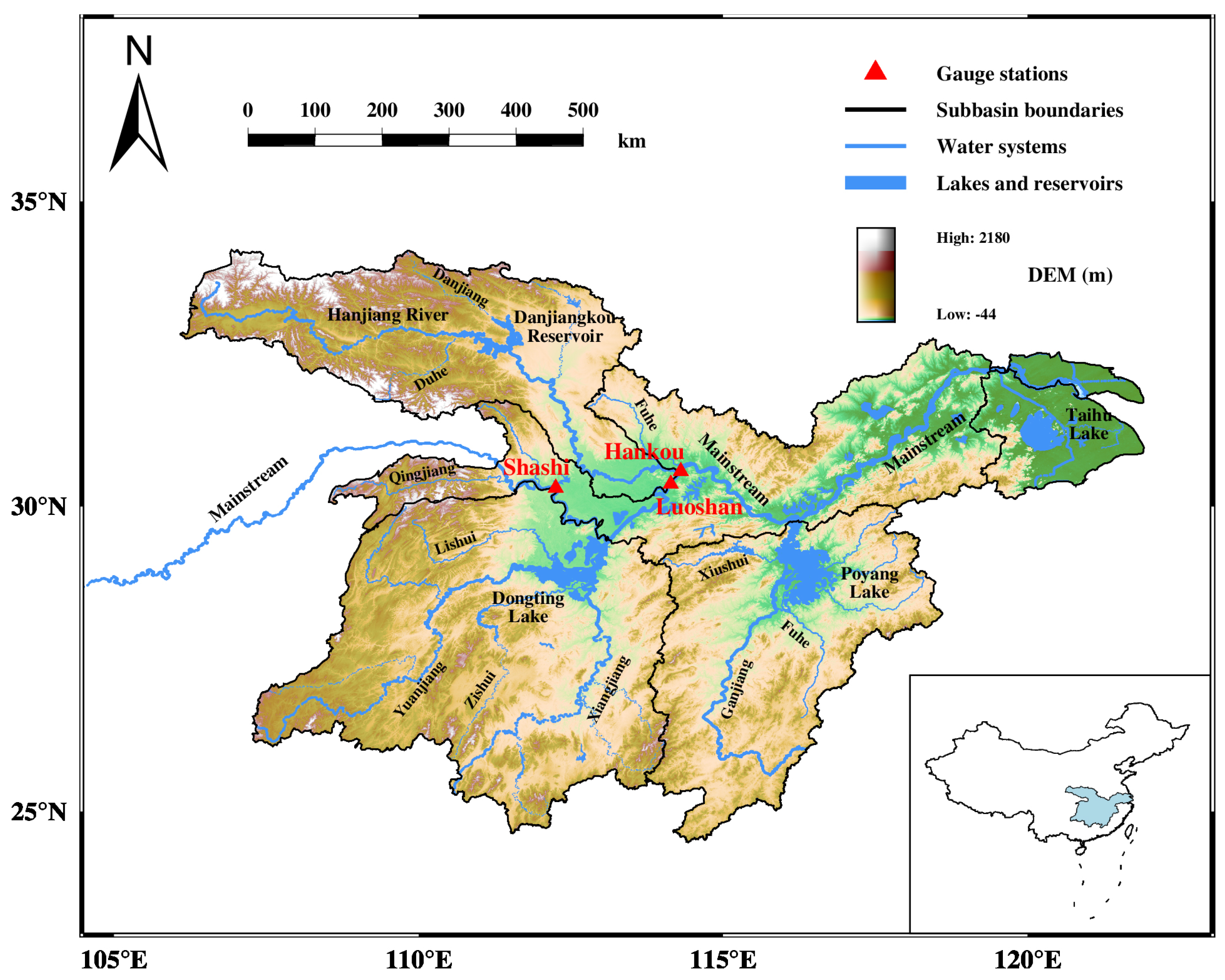
2.1.1. Study Region and Datasets

As shown in Figure 1, the river reaches of the Hankou, Shashi, and Luoshan hydrometric stations in the middle and lower reaches of the Yangtze River basin are selected as the study regions because there are no tributary confluences and their river widths change significantly.

The time series of the gauged discharges of the three hydrometric stations were downloaded from the official website of the Hubei Hydrology and Water Resources Center, available at http://113.57.190.228:8001/web/Report/RiverReport (accessed on 14 March 2023), and these data will be used as a benchmark to evaluate the results of the discharge estimation methods used in this paper. In addition, Landsat 8 remote-sensing images without cloud cover from 2013 to 2021 were downloaded from the United States Geological Survey (USGS), available at https://earthexplorer.usgs.gov/ (accessed on 14 March 2023), to extract river-shape information and then used for the SWOT-river-product simulation.

2.1.2. SWOT-River-Product Simulation

The SWOT mission is the first satellite altimetry mission that provided the very first comprehensive view of Earth’s freshwater bodies from space. The Ka-band Radar Interferometer (KaRIn) carried by SWOT can simultaneously realize the high spatial and temporal resolution monitoring of the terrestrial water surface, provide a global inventory of all terrestrial water bodies (lakes, reservoirs, wetlands) whose surface area exceeds 250 m by 250 m and rivers whose widths exceed 100 m, and obtain the water-surface-area measurement with a relative error of less than 15% [42]. SWOT is being jointly developed by NASA and CNES with contributions from the Canadian Space Agency (CSA) and United Kingdom Space Agency. SWOT, launched on 16 December 2022, is currently in Phase D (i.e., checkout).

SWOT features a high-rate (HR) data mode for continental hydrology. The SWOT_ HYDROLOGY_ TOOLBOX is a simulator released by CNES for simulating SWOT inland river and lake HR data together with JPL’s RiverObs tool. It can be downloaded at https://github.com/CNES/swot-hydrology-toolbox (accessed on 14 March 2023). This simulator can run on Linux, Mac, and Windows systems after a series of configurations. For more details, please refer to the user manual CNES Large Scale SWOT Simulator [43]. In this paper, the main inputs of the simulator are the polygon shapefiles of the river reaches, satellite orbit data, the start time of the mission, and the output is the “pixel cloud” product, which is one of the original terrestrial hydrology products of SWOT.

This paper uses 44 Landsat 8 remote-sensing-image data from 2013 to 2021 to simulate SWOT-river-product data based on the SWOT_ HYDROLOGY_ TOOLBOX provided by CNES. Firstly, river polygon vector data of three river reaches (each of them is about 10 km) are extracted from all Landsat 8 images. Secondly, the polygon vector data are edited according to the user manual (the main purpose of this paper is to extract the river width from the simulated SWOT river products, so no water-surface-height information is added to the polygon vector data). Finally, the polygon vector data is taken as the input data of the SWOT_ HYDROLOGY_ TOOLBOX to simulate the SWOT “pixel cloud” product (as shown in Figure 2a).

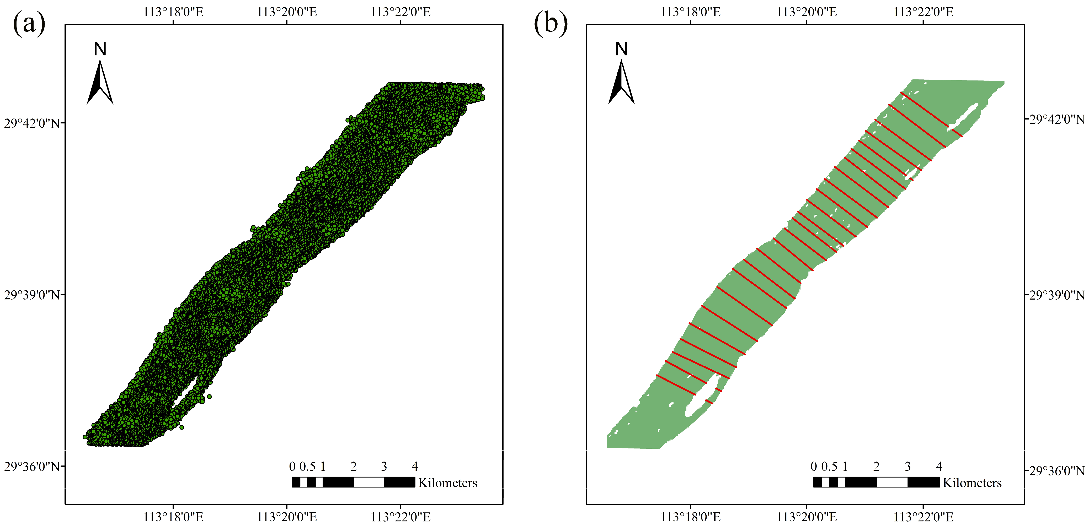
2.1.3. River-Width Extraction from SWOT River Product

The simulated SWOT-river-product data are a “pixel cloud” product. Firstly, in order to extract the river width, the simulated “pixel cloud” product needs to be clustered to get the river polygon information of the whole river reach (green area in Figure 2b). Then, the boundary polygon of the river and the river cross-sections with approximately equal intervals are used to obtain the intersection part of each cross-section and the river reach (the red solid line in Figure 2b). Finally, the length of the intersections is calculated, then the river-width time series of each cross-section of the three river reaches can be obtained (as shown in

Table 1. River width of 25 cross-sections of the Luoshan reach on 2 May 2021.

Cross-Section No.	Width (m)	Cross-Section No.	Width (m)
1	2028.23	14	1490.06
2	2027.54	15	1490.46
3	1922.89	16	1625.91
4	1875.83	17	1877.38
5	1758.96	18	1941.77
6	1967.31	19	1938.64
7	1882.49	20	1901.33
8	1966.83	21	1822.39
9	1899.51	22	1790.99
10	1840.87	23	1764.48
11	1740.1	24	1447.5
12	1648.15	25	1439.12
13	1590.08

).

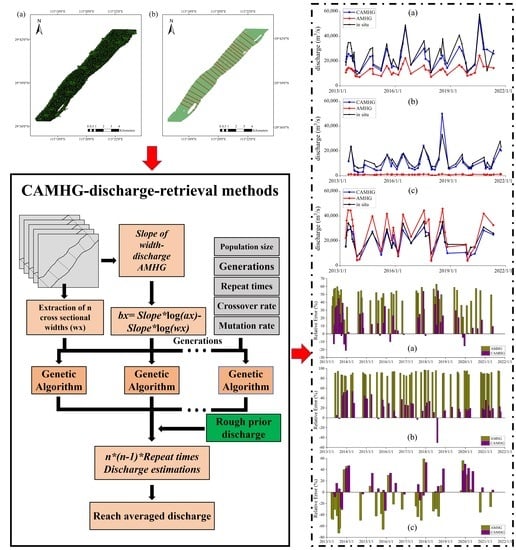
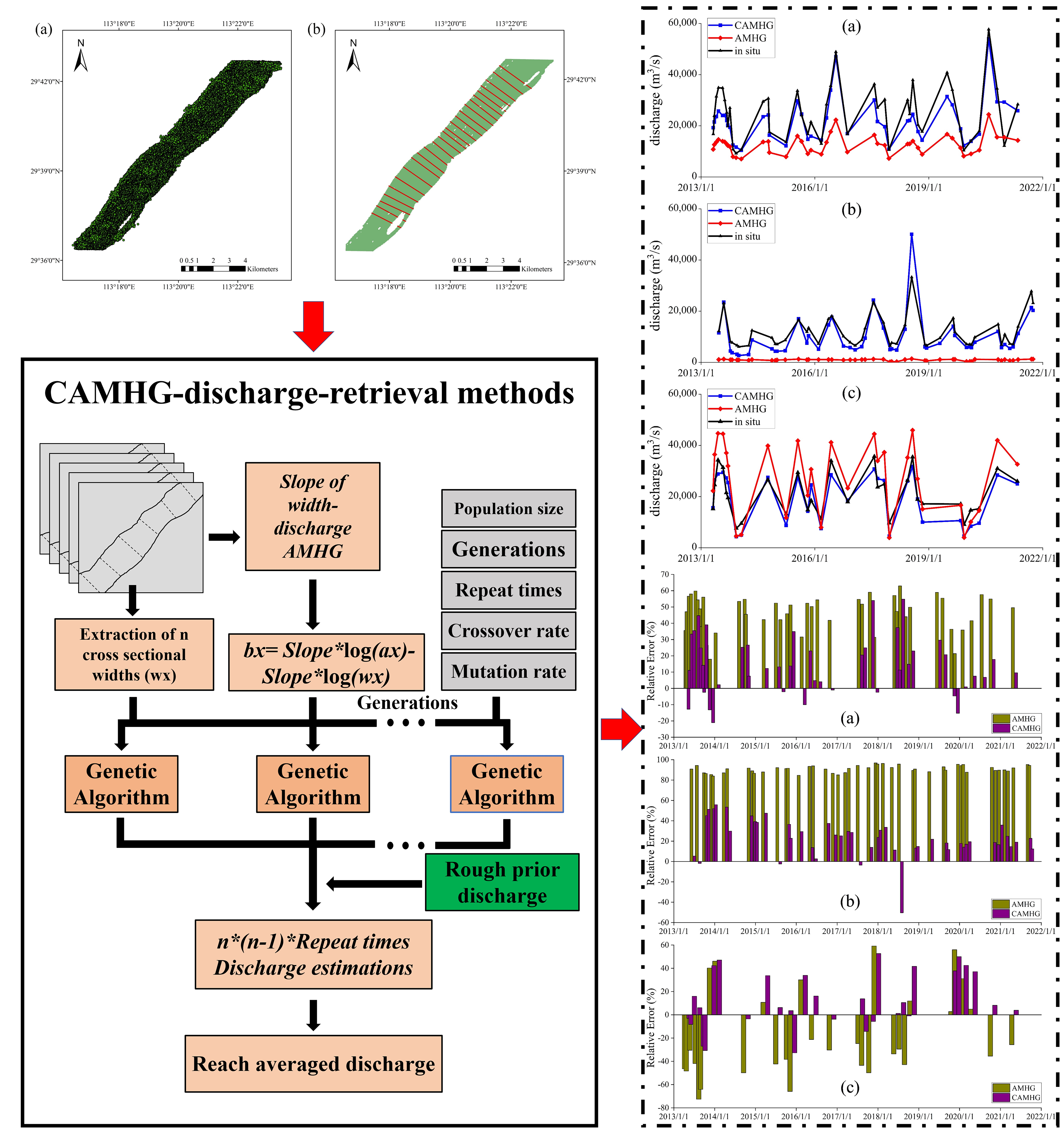
2.2. AMHG-Discharge-Retrieval Methods

2.2.1. At-Many-Stations Hydraulic Geometry

The AHG (Equations (1)–(3)) was first proposed by Leopold and Maddock [44], which is a very practical tool for various hydrological analyses, and the width-discharge relationship (Equation (1)) is widely used in the field of river remote sensing [16,18,45]. Equations (4) and (5) describes the relationship between the AHG coefficients a, b, c and exponents b, f, m. It is worth noting that not all locations on the river can show a significant AHG relationship, because the form of the AHG is too simple to properly express the hydraulic characteristics of all locations on the river. In addition, the AHG relationship is only effective when the flow is maintained in the river channel.

$$W=a\cdot Q^b$$

(1)

$$Y=c\cdot Q^f$$

(2)

$$U=k\cdot Q^m$$

(3)

$$a\cdot c\cdot k=1$$

(4)

$$b+f+m=1$$

(5)

where W denotes the river width, Y denotes the river depth, U denotes the water velocity, Q denotes the river discharge, a, c, and k denote the AHG coefficients, and b, f, and m denote the AHG exponents.

The AMHG was proposed by Gleason and Smith [26], and it is believed that the coefficients and exponents of the AHG are stable and predictable for a given river, and the relationship between the AHGs of the cross-sections has been established. Gleason and Smith found that there is a logarithmic linear relationship between the coefficient and exponent of the AHG at each cross-section of the same river (Equation (6)), which was proved by the measured width (w), depth (d), speed (v), and flow (Q).

$$F=a_{x1,x2,\dots ,xn}{E}^{b_{x1,x2,\dots ,xn}},$$

(6)

where a and b are the AHG parameters of each cross-section, and F and E are constants related to the AMHG intercept and slope that remain unchanged for a given river.

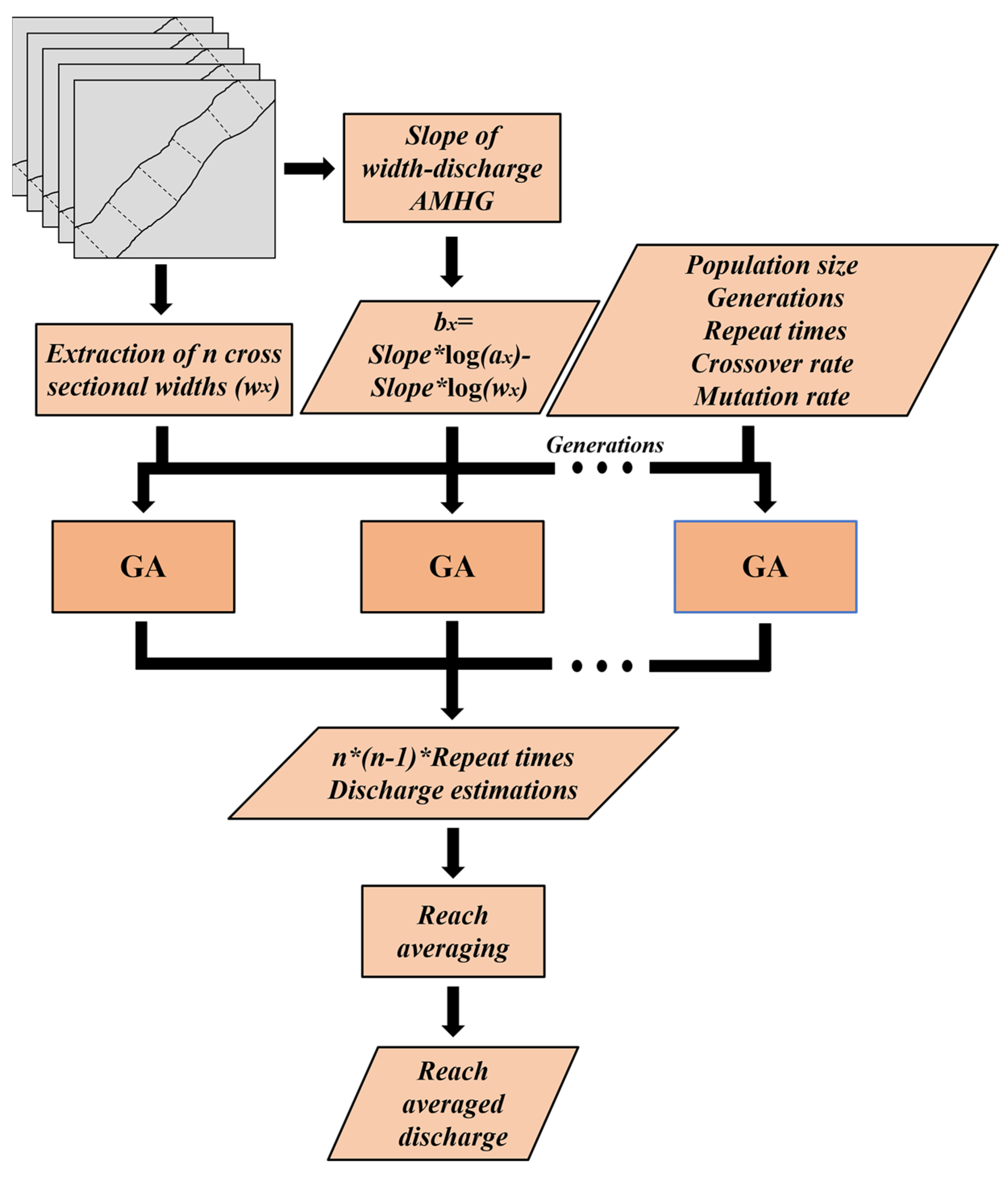
2.2.2. Discharge-Calculation Workflow Based on AMHG and SWOT River Width

In this paper, we take the Hankou reach of the Yangtze River as an example to illustrate the flow-calculation process based on the SWOT river width and the AMHG method. The calculation process is divided into two steps. The first step is to establish the AMHG relationship of the river reach, and the second step is to calculate the discharge using the established AMHG and the river width provided by SWOT. The calculation workflow is shown in Figure 3.

(1) Establishment of the AMHG relationship. Firstly, the Hankou reach is divided into 10 segments, and 11 cross-sections perpendicular to the river-flow direction are obtained. Then, using the SWOT river widths at 11 cross-section locations and the measured discharge of the Hankou hydrometric station, the AHG parameters (i.e., a and b) of each cross-section are fitted according to Equation (1). Finally, the AMHG relationship of the Hankou reach of the Yangtze River can be obtained by the logarithmic linear fitting of log a and b of 11 cross-sections (the black solid line in Figure 4).

(2) The discharge calculation combining the AMHG-discharge-retrieval method and the SWOT river width. After the AMHG relationship of the Hankou reach is obtained, the discharge can be calculated by combining it with the river width. The GA is the key to calculate the river discharge solely using the SWOT river width in this paper. The GA is a numerical optimization method which simulates the process of natural selection, mutation, and sexual reproduction through the interaction of basic units termed “genes” and “chromosomes” [27]. The GA used in this paper is similar to that used by Gleason and Smith [26], and includes five steps (the parameter settings of the GA are shown in

Table 2. Parameterization of the genetic algorithm used in this study.

Parameter	Value
Population size	10
Generations	50
Minimum value of coefficient a	10
Maximum value of coefficient a	1000
Minimum value of exponent b	0.01
Maximum value of exponent b	0.31
Crossover rate	0.8
Mutation rate	0.1
Minimum allowable discharge	5000 m3/s
Maximum allowable discharge	60,000 m3/s
Repeat times	50

).

Step 1. Randomly take 2 of 11 cross-sections, where each cross-section has two parameters (i.e., a and b) that needs to be evaluated, which are called the genes of the chromosome, that is, a chromosome that has four genes. The GA starts with 10 such chromosomes, where each gene of the chromosome (a or b) is randomly drawn from a reasonable value range defined by a narrow envelope surrounding the empirically derived width AMHG (Table 2). Then, the chromosomes are combined with the observed widths to calculate the discharge. Chromosomes that generate discharges falling outside of the allowable discharge are discarded. Any chromosome that is discarded for generating an unreasonably large or small discharge is replaced by a new chromosome randomly drawn from the solution space until all 10 chromosomes pass the discharge filter. Chromosomes are then sorted according their “fitness” (fitness is calculated as the percentage difference in the discharge between the two cross-sections represented by the chromosome). After that, each chromosome has the opportunity to undergo the processes of “crossover” and “mutation”. In crossover, the specific genes of specific chromosomes will be exchanged. In mutation, there is a small chance that the genes will be randomly changed. The altered chromosomes are then reranked by their fitness, and the five chromosomes with the lowest fitness will be discarded and replaced with randomly generated chromosomes that meet the AMHG solution space. After the above processes, the initial 10 chromosomes have completed one generation. When the GA runs for fifty generations, two pairs of optimal AHG parameters can be obtained.

Step 2. Repeat Step 1 50 times to obtain 100 pairs of optimal AHG parameters.

Step 3. All possible pairwise combinations of the 11 cross-sections are carried out in Steps 1 and 2 to obtain n (n − 1) ∗ 100 pairs of optimal AHG parameters. Moreover, each cross-section has (n − 1) ∗ 100 pairs of optimal AHG parameters, where n is the number of cross-sections.

Step 4. Extract the median value of coefficient a or exponent b for each cross-section from its optimal AHG parameters, and then substitute them into the AMHG relationship to obtain the corresponding exponent b or coefficient a.

Step 5. The time series of the AHG coefficient a and exponent b obtained by Step 4 and the SWOT river widths can be substituted into Equation (7) to obtain the discharge time series of each cross-section, and then the discharge of the 11 cross-sections can be averaged to obtain the reach-averaged discharge of the Hankou reach.

$$Q={10}^{(\frac{\log (W)-\log (a)}{b})}$$

(7)

where W is the time series of the river width, a is the AHG coefficient, and b is the AHG exponent.

However, in practical application, especially in remote areas, the AMHG relationship cannot be established due to the lack of a gauged discharge. At this time, a special method can be used to determine the AMHG relationship of a river reach. Gleason and Smith [26] provided a method (Equation (8)) to obtain the AMHG relationship by only fitting the river width. Firstly, the index y is obtained by fitting the river width with Equation (8). Because the index y has a good approximate relationship with the slope of the AMHG, the slope of the AMHG can be obtained by taking a negative number for y. Then, the intercept of the AMHG can be calculated by using the relationship between the intercept and slope (Equation (9)). Finally, the AMHG relationship of the reach is established by only using the river width (i.e., the red dotted line in Figure 4 and Equation (10), where the slope and intercept in Equation (10) only represent the Hankou reach of the Yangtze River). In this paper, the AMHGs of the Hankou, Shashi, and Luoshan reaches are established according to this method, and then the discharge estimations are obtained according to the above AMHG-discharge-calculation workflow (Figure 3) and compared with the gauged discharge.

$$\max (w_{x1,x2,\dots ,xn})=p{(\max {(w_{x1,x2,\dots ,xn})}^2-\min {(w_{x1,x2,\dots ,xn})}^2)}^y$$

(8)

$$intercept=-slope\ast \log (w_x)$$

(9)

where $w_{x1,x2,\dots ,xn}$ indicate the river widths of each cross-section, index y has a good approximate relationship with the slope of AMHG, the slope is the opposite of the exponent y, and $w_x$ is the average of the river width of all cross-sections in this reach.

$$b=-0.30478*{\log }_{10}(a)+0.9161$$

(10)

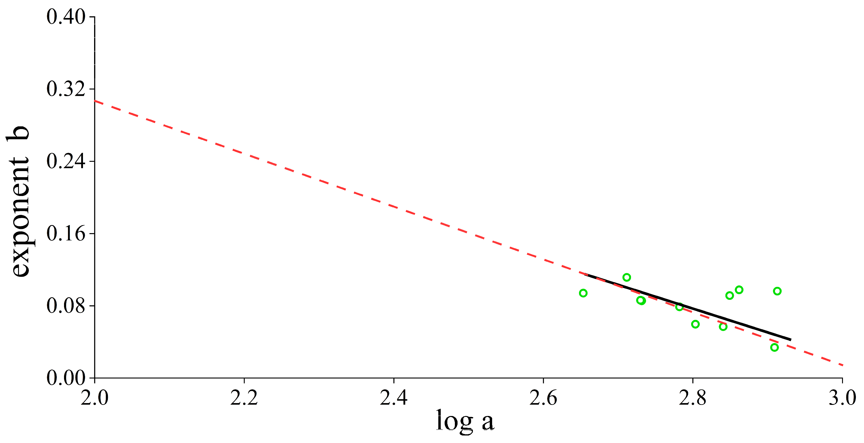
2.2.3. Constrained At-Many-Stations Hydraulic Geometry-Discharge-Retrieval Approach

In the introduction, it is mentioned that many scholars have recognized the shortcomings of the original AMHG-discharge-retrieval method and have attempted to improve the accuracy of the discharge estimation. Compared with the original AMHG method, the attempts have improved the accuracy of the discharge estimation, but there still exist the bias in the estimated and gauged discharge, as well as the accuracy difference of the estimated discharge in the dry season and wet season.

Gleason and Smith [26], Gleason et al. [27], and Gleason and Wang [28] used the approach of setting the discharge-tolerance range of a river discharge in the GA to control the AHG coefficient a and exponent b within a reasonable range, but the discharge-tolerance range can only be set accurately according to the historical dataset of the gauged discharge. However, in unmonitored regions, this tolerance range may be set unreasonably. As a result, despite the coefficient a and exponent b of the AHG given by the GA being consistent with the AMHG relationship, they are not consistent with the truth situation of the river reach, and the river discharge calculated according to them may have a large deviation.

Therefore, if an additional constraint condition (i.e., a numerical value that can approximately represent the discharge of the river reach) is added in the original AMHG-discharge-retrieval approach, to obtain AHG parameters which are more consistent with the truth situation of the river reach, thus improving the accuracy of the discharge estimation. The detailed steps are as follows: First, the AHG parameters given by the GA are used to calculate the discharge. Then, the estimated discharge is compared with the prior-constrained discharge. When the absolute value of the difference between the estimated and prior-constrained discharge is less than 20% of the prior-constrained discharge, preserve the corresponding AHG coefficient a and exponent b are retained, otherwise they are discarded. Finally, the filtered AHG parameters are used to calculate the river discharge of each cross-section, and the reach-averaged discharge is taken to represent the final result.

2.2.4. Performance Metrics

In this paper, four metrics are used to assess the performance of the AMHG-discharge retrieval-methods (

Table 3. Performance metrics used for the evaluation of AMHG discharge estimation.

Description	Abbreviation	Definition
Relative error	RE	$\frac{Q_i-{\widehat{Q}}_i}{{\widehat{Q}}_i}$
Root-mean-square error	RMSE	$\sqrt{\frac{1}{N}{\displaystyle \sum _{i=1}^N{(Q_i-{\widehat{Q}}_i)}^2}}$
Relative-root-mean-square error	RRMSE	$\sqrt{\frac{1}{N}{\displaystyle \sum _{i=1}^N{(\frac{Q_i-{\widehat{Q}}_i}{Q_i})}^2}}$
Correlation coefficient	CC	$\frac{\mathrm{cov}(Q,\widehat{Q})}{\sqrt{\mathrm{var}(Q)\mathrm{var}(\widehat{Q})}}$ 1

¹ cov is the covariance between estimated and gauged discharge, and var is variance of estimated or gauged discharge.

). Relative error (RE) is the ratio of absolute error (i.e., the estimated discharge minus the gauged discharge) to the truth value. The root-mean-square error (RMSE) measures the deviation between the estimated value and the gauged value. The relative-root-mean-square error (RRMSE) is the root-mean-square of the relative error. The correlation coefficient (CC) measures the degree of correlation between the estimated value and the gauged value.

3. Results

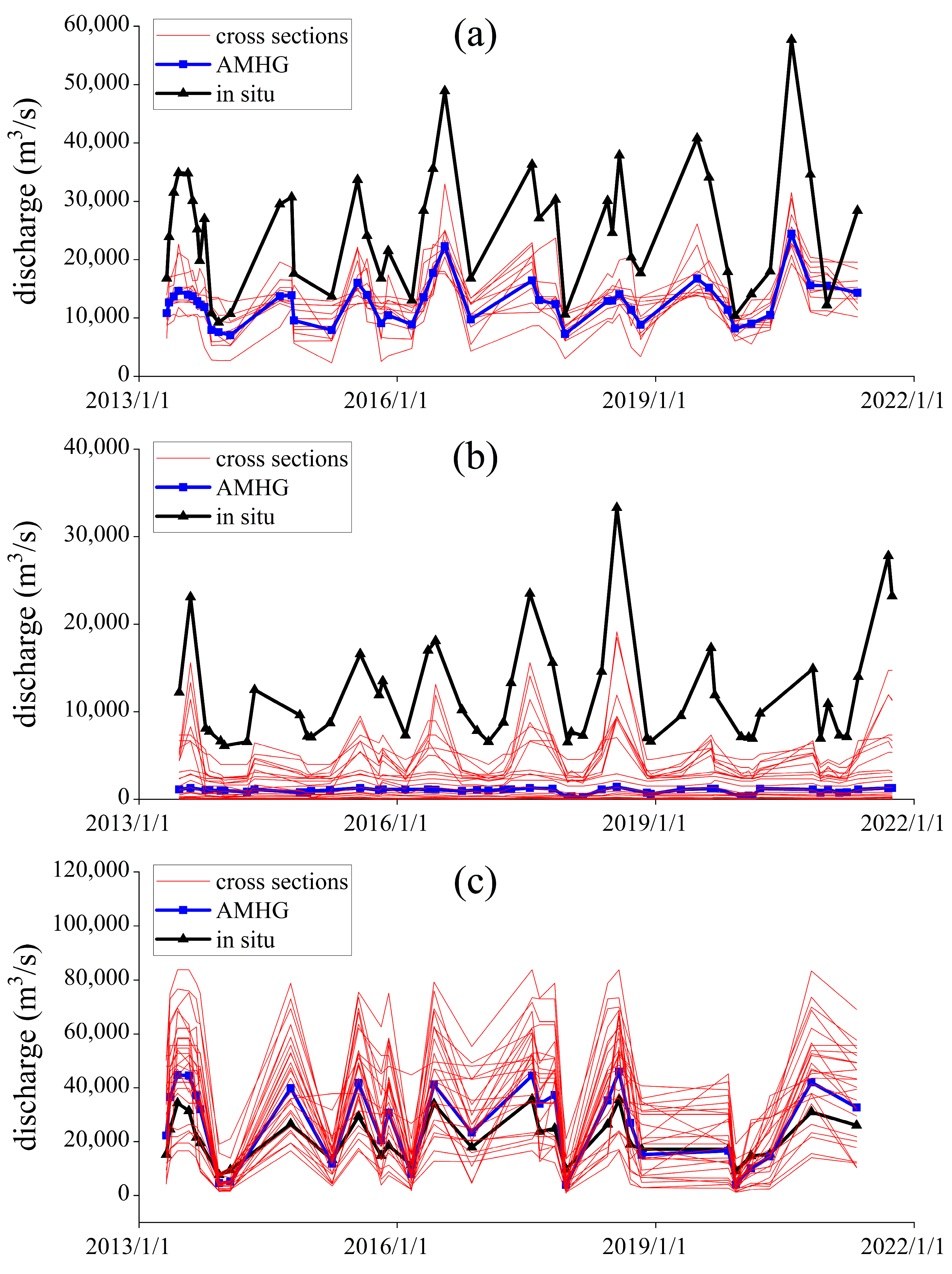
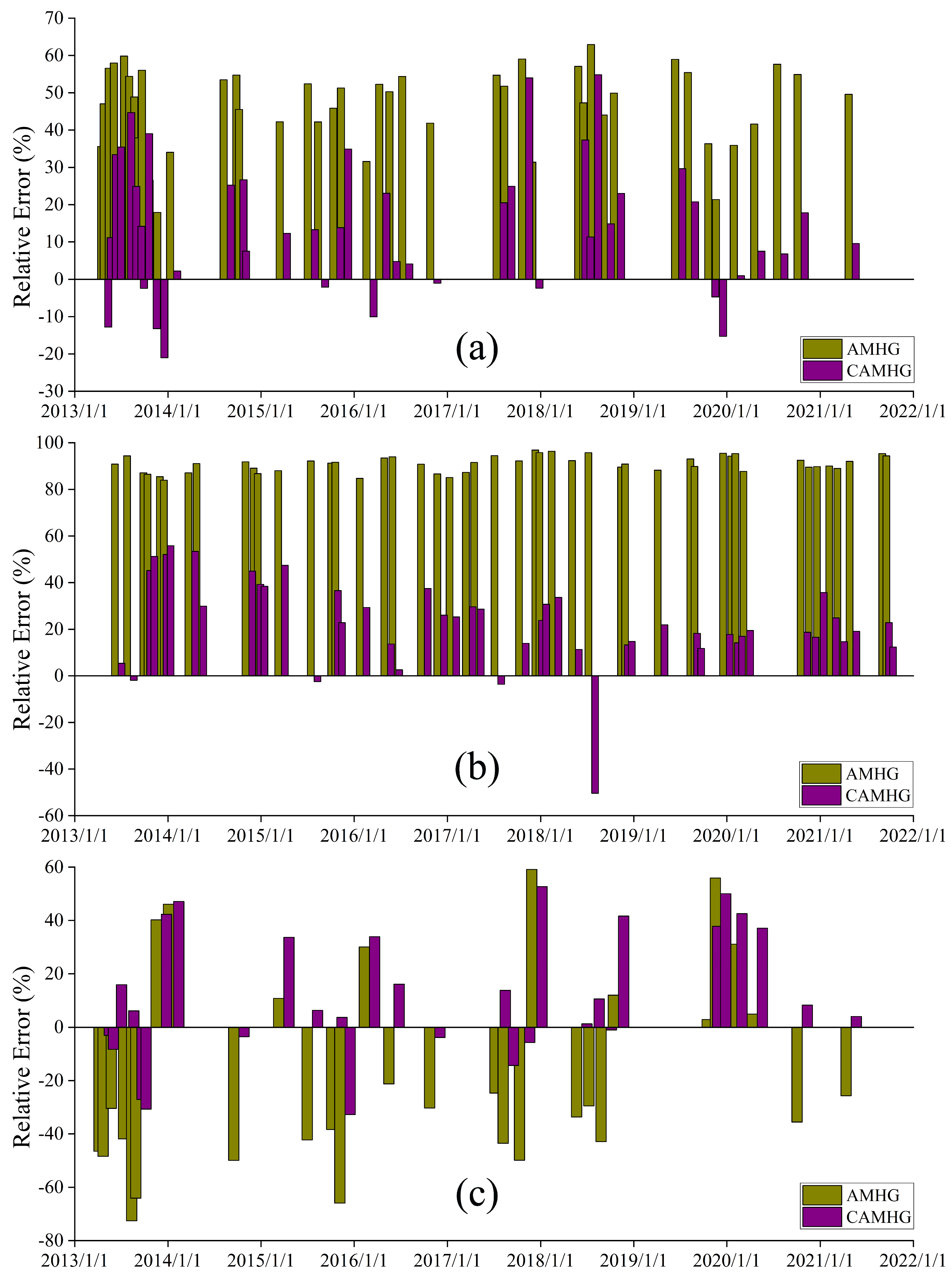
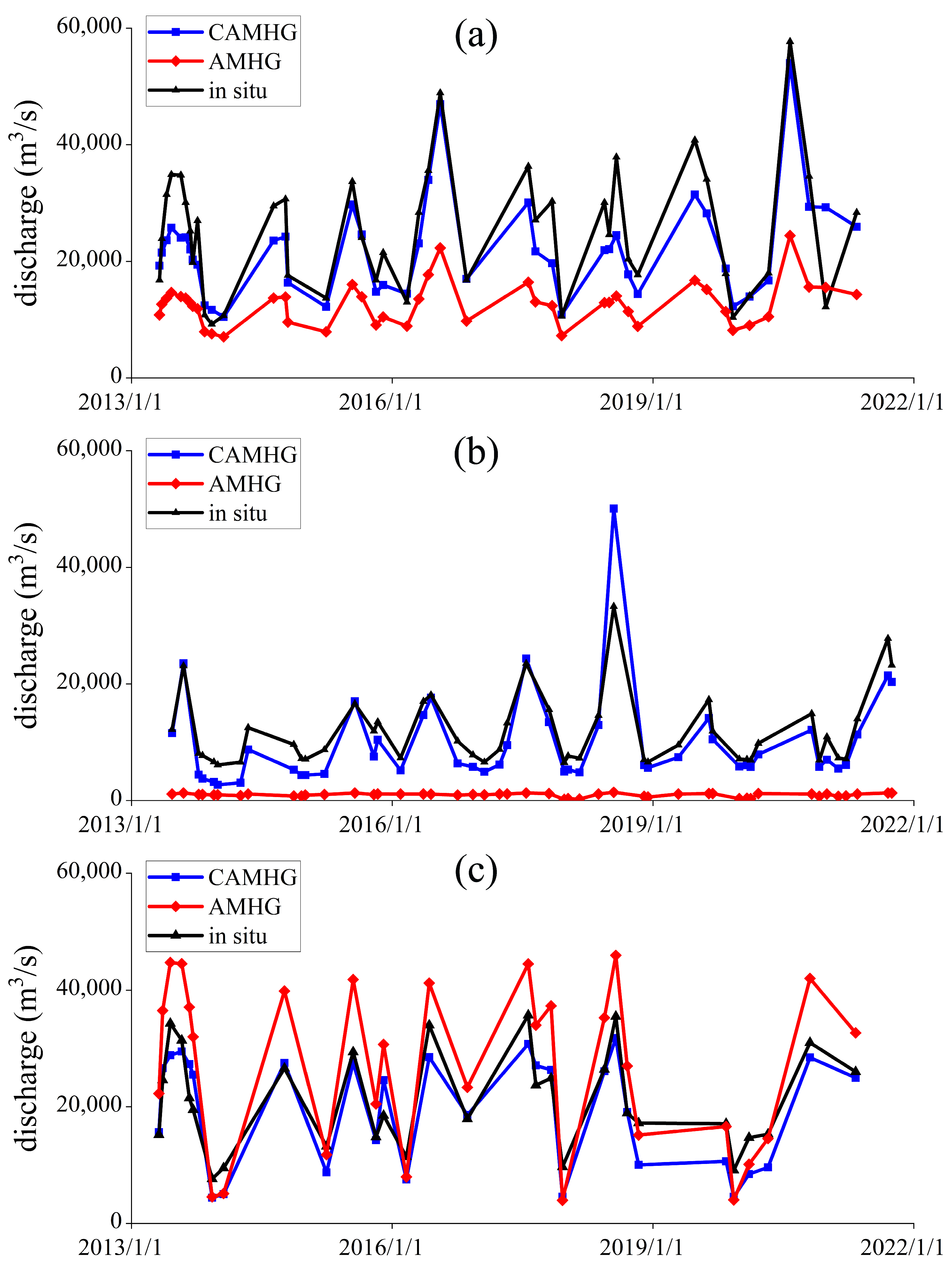
3.1. Discharge Estimation of Original AMHG-Discharge-Retrieval Method

In the three reaches of the middle and lower reaches of the Yangtze River basin, the AMHG-discharge-retrieval method is combined with the simulated SWOT river widths to calculate the river discharge according to the method described in Section 2.2.2, and the estimated discharge is compared with the gauged discharge at the hydrometric station. The results are shown in Figure 5a.

The same method is used to estimate the discharge of the Shashi and Luoshan reaches of the Yangtze River, and then the results are compared with the gauged discharge. The results are shown in Figure 5b,c.

It can be seen from Figure 5 and

Table 4. Statistics of discharge estimation by original and CAMHG-discharge-retrieval methods.

Reach	AMHG			Optimized AMHG
	RMSE (m3/s)	RRMSE	CC	RMSE (m3/s)	RRMSE	CC
Hankou	14,628.958	100.1%	0.9157	5784.471	24.4%	0.8925
Shashi	12,298.872	1137.1%	0.6484	4131.544	49.9%	0.9487
Luoshan	8852.526	48.6%	0.9489	4143.641	45.5%	0.9179

that the original AMHG-discharge-retrieval method can be used to calculate the river discharge solely using the SWOT-river-width data. The estimated discharge similar to the variation trend of the gauged discharge can be obtained, and the CCs in the Hankou, Shashi, and Luoshan reaches are 0.9157, 0.6484, and 0.9489, respectively. However, the accuracy of the estimated discharge is limited compared with the gauged discharge, and the RMSEs for the Hankou, Shashi, and Luoshan reaches are 14,628.958 m³/s, 12,298.872 m³/s, and 8852.526 m³/s, respectively, and the RRMSEs for these three reaches are 100.1%, 1137.1%, and 48.6%, respectively.

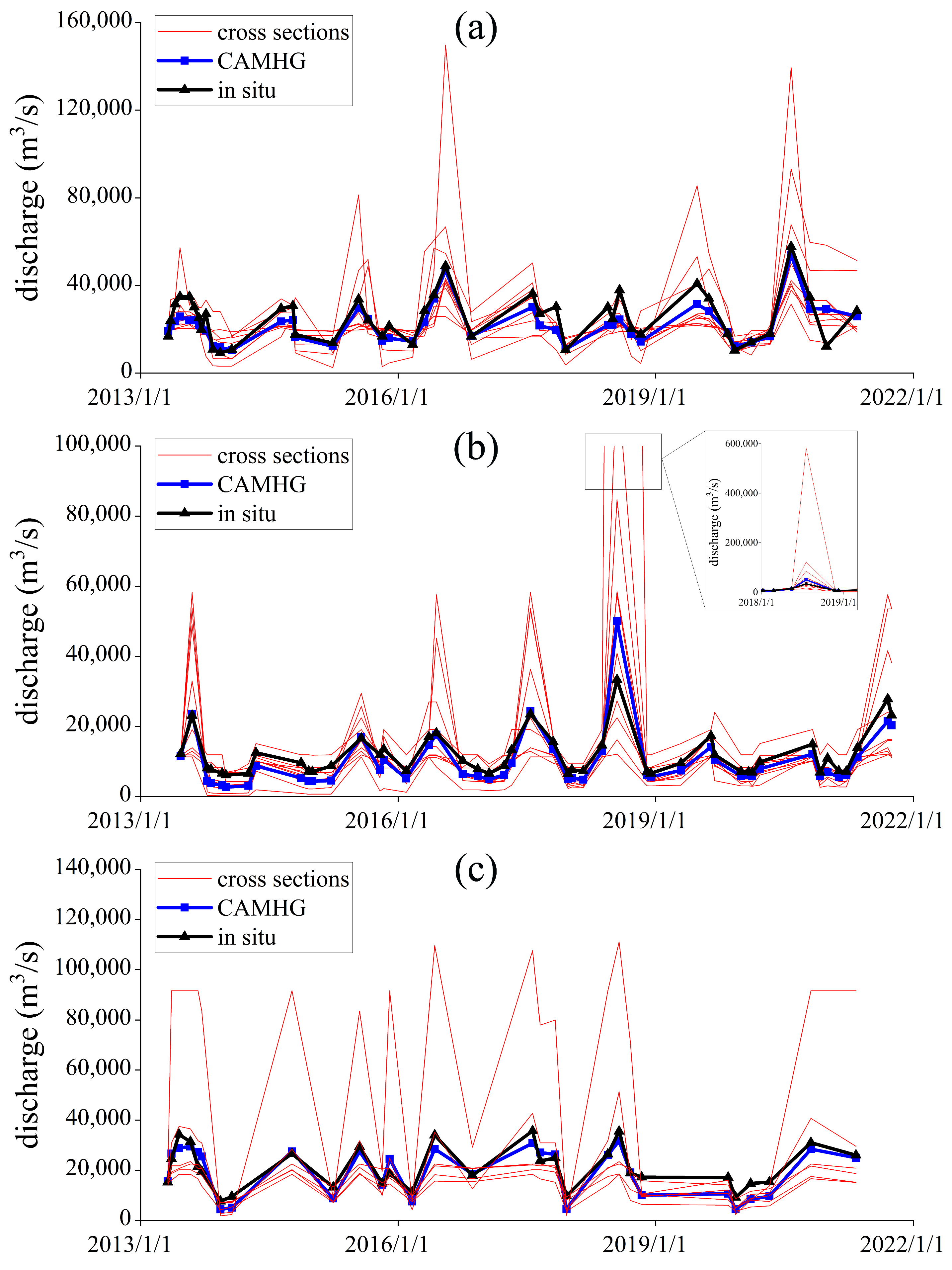
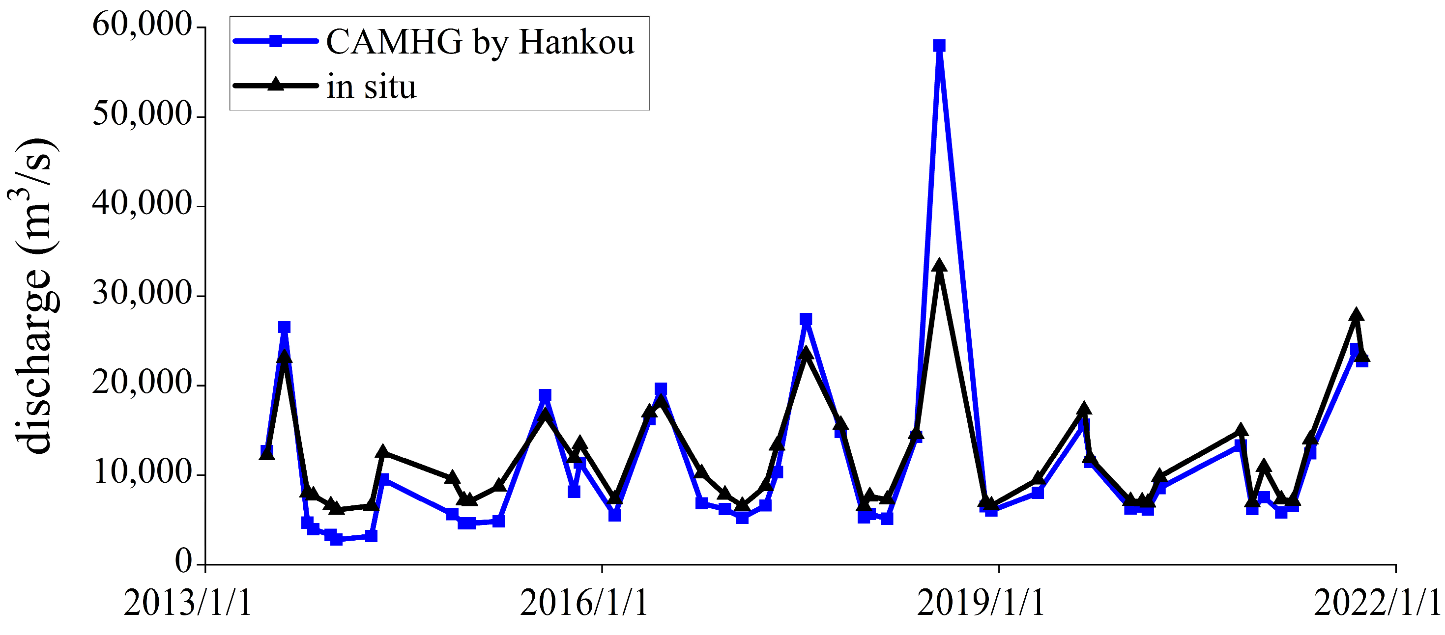
3.2. Discharge Estimation of CAMHG-Discharge-Retrieval Approach

An approximate prior discharge is used to constrain the GA of the original AMHG-discharge-retrieval approach to obtain a more accurate AHG coefficient a and exponent b. Then, the river discharge is calculated by the filtered AHG parameters and the SWOT river widths and compared with the gauged discharge. The results of the CAMHG-discharge-retrieval approach in the Hankou, Shashi, and Luoshan reaches are shown in Figure 6a–c, respectively.

It can be seen from Figure 6 that, in the Hankou, Shashi, and Luoshan reaches, the discharge calculated by the CAMHG-discharge-retrieval approach can match the gauged discharge with higher accuracy. As shown in Table 4, the RMSEs are 5784.471 m³/s, 4131.544 m³/s, and 4143.641 m³/s, respectively, the RRMSEs are 24.4%, 49.9%, and 45.5%, respectively, and the CCs are 0.8925, 0.9487, and 0.9179, respectively.

4. Discussion

4.1. Analysis the Results of Original AMHG-Discharge-Retrieval Method

From Figure 5 and Table 4, it is found that there is a large gap between the discharge estimated by the original CAMHG-discharge-retrieval method and the gauged discharge, and the gap shows a significant systematic gap in the Hankou and Shashi reaches (as shown in Figure 7a,b). The RE in the Hankou reach is between 10% and 70% (Figure 7a), and the RE in the Shashi reach is greater than 80% (Figure 7b).

In addition, it can also be found in Figure 5 that the difference between the estimated and gauged discharge is smaller in the dry season and larger in the wet season, which is consistent with the conclusions of previous research [26,28].

In view of the fact that the original AMHG-discharge-retrieval approach cannot accurately estimate the magnitude of the river discharge, and the estimation accuracy also has seasonal differences, the original AMHG approach combined with SWOT-river-width data may not meet the requirements of practical application, so it should be improved. The reasons for the insufficient estimation of the discharge are: the AMHG relationship itself is too simple to stably describe the hydraulic geometric relationship of all river cross-sections; the change of the river discharge in the study regions cannot cause significant changes in the river width; the measurement error of the river width and the calculation error of the AHG parameters. The first two of these belong to the inherent deficiencies of the AMHG. Ignoring the error of the river width, this study starts by weakening the calculation error of the AHG parameters to improve the accuracy of the estimated discharge by combining the SWOT river width with the AMHG method. The scheme adopted is to control the accuracy of the AHG parameters given by the original AMHG with a prior discharge as the constraint condition (as shown in Section 2.2.3).

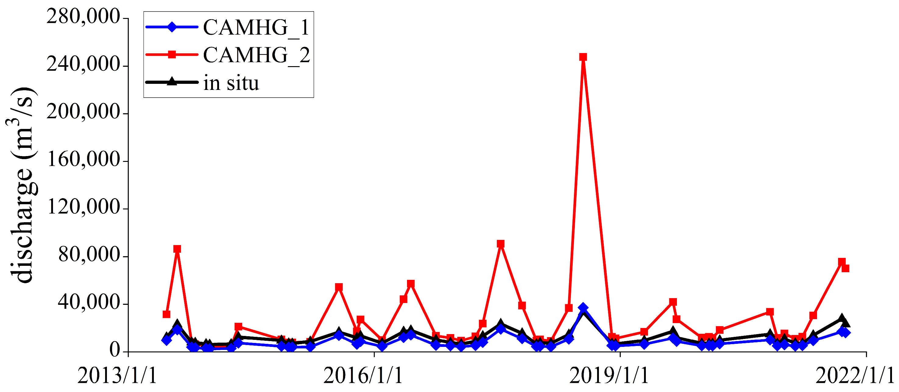
4.2. Analysis of the Results of the CAMHG-Discharge-Retrieval Approach

When estimating river discharge under the constraint of the prior discharge, the selection of the prior discharge and the threshold value will control how many cross-sections can participate in the final discharge calculation of the river reach. Some cross-sections of the river reach are excluded from the discharge calculation by the prior discharge because of they have no significant AHG relationships, thus improving the discharge accuracy of the river reach.

It can be seen from Figure 8 that, in the Hankou, Shashi, and Luoshan reaches, the discharge estimated by the CAMHG-discharge-retrieval approach (the red solid line in Figure 8) is closer to the gauged discharge (the black solid line in Figure 8) than the discharge calculated by the original AMHG-discharge-retrieval method (the blue solid line in the Figure 8). In Table 4, it clearly shows that the discharge estimated by the CAMHG-discharge-retrieval approach has a smaller RMSE and RRMSE than that of original AMHG method. In addition, it also can be seen from Figure 8 that the seasonal accuracy difference of the discharge estimated by the CAMHG method also becomes smaller. In this study, we divided May to September as the wet season and November to March as the dry season, and then analyzed the ability of the CAMHG method to improve the seasonal difference of the discharge estimation. It can be seen from

Table 5. Comparison of the discharge estimation accuracy between the original and CAMHG-discharge-retrieval method in the wet season and dry season.

Reach	RMSE_Wet (m3/s)		RMSE_Dry (m3/s)
	Before	After	Before	After
Hankou	17,967.503	6047.949	6183.772	3857.448
Shashi	18,475.323	5295.306	6923.751	2510.011
Luoshan	11,221.269	3529.366	4177.478	4647.384

that, in the wet season, the discharge estimation accuracy of the AMHG method constrained by the prior discharge is about three times higher than that of the original AMHG method. In the dry season, the improvement of the discharge estimation accuracy is not significant, and the discharge estimation accuracy of the CAMHG-discharge-retrieval approach in the Luoshan reach is even equivalent to that of the original AMHG method. The experimental results show that the CAMHG approach has a higher discharge estimation accuracy than that of the original AMHG method, and also has the ability to weaken the seasonal difference of the discharge estimation accuracy, and likely has strong applicability in different river reaches.

4.3. Influence of Prior Discharge and Threshold Selection on Discharge Calculation

It is found in this paper that the principle of proximity should be followed when setting the prior discharge; that is, the historical observation data of the river reach or the adjacent river reach should be used as the prior discharge. If the prior discharge setting is unreasonable, the discharge estimation accuracy of the CAMHG-discharge-retrieval approach may become worse.

Figure 9 shows the comparison of the CAMHG discharge estimations constrained by the annual average discharge of the Shashi hydrometric station and the Yangtze River estuary at the Shashi reach. It can be seen from the figure that, when the annual average discharge of the Yangtze River estuary is used as the prior discharge, a worse discharge estimation is obtained because the annual average discharge of the Yangtze River estuary is far greater than the annual average discharge of the Shashi reach.

In this paper, the prior discharge used in the Hankou, Shashi, and Luoshan reaches is the annual average discharge calculated from the historical observation data of their corresponding hydrometric stations. When the historical observation data of a river reach cannot be obtained, the prior discharge can also be obtained from the historical observation data of its adjacent upstream or downstream river reaches. As can be seen from Figure 10, using the historical observation data of adjacent hydrometric stations for the constraint of the GA can also obtain better discharge estimation results, and the closer the river reach providing the prior discharge is to the river reach to be calculated, the higher the accuracy of the discharge estimation will be. When there is no historical discharge data on the whole river, the approximate prior discharge can be given by the discharge data of other rivers using the relationship between the discharge and drainage area. In addition, after the launch of SWOT, the river discharge can be calculated solely using SWOT measurements [1,36,38], which can also be used as the prior discharge to constrain the GA process of the AMHG-discharge-retrieval approach.

Moreover, after setting the prior discharge reasonably, in order to obtain a more accurate discharge, the threshold value is not set as small as possible. It is found from

Table 6. Comparison of discharge estimation results under different thresholds.

Threshold	RMSE (m3/s)	CC
50%	4411.595	0.9504
20%	3649.598	0.9412
10%	3798.167	0.9398
5%	3864.888	0.9394

that, when the threshold value is 20% of the prior discharge, compared with the others, the RMSE between the estimated discharge and the gauged discharge is the minimum, and the CC is also high enough. When the threshold value is set smaller than 20%, the RMSE increases and the CC decreases. Therefore, this study sets the threshold value as 20% of the prior discharge.

4.4. The Feasibility of Establishing AMHG Relationship Solely Using River-Width Data

Gleason and Wang [28] pointed out that the method of establishing the AMHG relationship by only using the river width is not perfect and is not applicable to some rivers. However, in this paper, only SWOT-river-width data are used to establish the AMHG relationships in the three reaches of the middle and lower reaches of the Yangtze River. It can be seen from Figure 4 and Figure 11 that AMHG relationships in the Hankou, Shashi, and Luoshan reaches that are solely fitted with the river widths have a good consistency with the AMHG relationships established through in-situ-measured data. After that, the AMHG relationship established solely using the river width is used for the discharge calculation. After the prior discharge is used for the constraint, the accuracy of the discharge estimation is better than that of the original AMHG method. Therefore, this paper believes that, in the middle and lower reaches of the Yangtze River, the method proposed by Gleason and Smith [26] and Gleason et al. [27] can be used to establish accurate AMHG relationships solely using the river-width data, and then more accurate AHG parameters can be obtained by using a prior discharge to constrain the GA of the original AMHG method, which further improves the accuracy of the discharge estimation. Therefore, the AMHG-discharge-estimation method based on a prior discharge constraint proposed in this paper can expand the application scope of the method proposed by Gleason and Smith [26] and Gleason et al. [27], and is expected to apply to more rivers.

It should be noted that the SWOT mission uses the difference between the backscattering coefficients of water and land to obtain the water-surface area. One of the scientific requirements of SWOT is that the RE of the water-surface-area observation is less than 15%. In addition, the along-track resolution of the SWOT data is about 5 m, and the cross-track resolution is about 10–70 m [42]. Therefore, the river-width accuracy obtained by the SWOT mission is likely different from that of the Landsat series remote-sensing satellites. In this paper, the Landsat 8 image data with a resolution of 30 m are used to simulate the SWOT data, which may not accurately represent the actual flow calculation accuracy of the SWOT.

5. Conclusions

In this paper, the simulated SWOT-river-width data and the AMHG-discharge-retrieval approach are used to jointly calculate the discharge. It is found that the discharge estimated by the original AMHG-discharge-retrieval method has a large deviation, the RMSEs of the river discharge are greater than 8852.526 m³/s, and the RRMSEs of the Hankou, Shashi, and Luoshan reaches are 100.1%, 1137.1%, and 48.6%, respectively. In addition, there also exists a difference in the accuracy of the discharge estimation in the dry season and wet season, i.e., the RMSE of the estimated discharge in the dry season is three times higher than that of the wet season. Based on the results of the analysis of the original AMHG-discharge-retrieval method, a CAMHG-discharge-retrieval approach constrained by a prior discharge is proposed in this paper, which can obtain AHG parameters that are more consistent with the truth situation of the river reach, and then improve the accuracy of the discharge estimation.

Our results show that the CAMHG-discharge-retrieval approach can obtain a more accurate discharge estimation than that of the original AMHG method, and the RMSEs of the discharge estimated by the CAMHG-discharge-retrieval approach are reduced to more than half of the original one, except for the Luoshan reach. Compared with previous research, the CAMHG-discharge-retrieval approach not only significantly improves the accuracy of the estimated discharge, but also reduces the difference between the accuracy of the discharge estimation in the dry season and the wet season, e.g., for the Hankou, the RMSE is 17967.503 m³/s for the wet season and 6183.772 m³/s for the dry season using the original AMHG-discharge-retrieval method; however, the RMSE is 6047.949 m³/s for the wet season and 3857.448 m³/s for the dry season using the CAMHG-discharge-retrieval approach.

In addition, Gleason and Wang mentioned that it is not recommended to use Equations (8) and (9) to estimate the AMHG relationship of the river reach. However, this paper found that the AMHG relationship calculated by Equations (8) and (9) was reasonable at three river reaches in the middle and lower reaches of the Yangtze River basin, and after using a priori discharge to constrain the AMHG-discharge-calculation process, a more accurate discharge estimation solely using remote-sensing data was achieved. Therefore, the CAMHG-discharge-retrieval approach proposed in this paper can further improve the applicability of the AMHG.

However, the applicability of the CAMHG-discharge-retrieval approach based on a constraint of prior discharge needs to be further evaluated globally. The detailed evaluation of the CAMHG-discharge-retrieval approach in different watersheds and geographical conditions is our future research goal.

In a word, based on the analysis of the shortcomings of the original AMHG-discharge-retrieval method, this paper proposes a remarkable CAMHG-discharge-retrieval approach constrained by prior discharge, which improves the application potential of the AMHG and can serve as the SWOT discharge calculation in the near future.

References

1. Durand, M.; Gleason, C.J.; Garambois, P.A.; Bjerklie, D.; Smith, L.C.; Roux, H.; Rodriguez, E.; Bates, P.D.; Pavelsky, T.M.; Monnier, J.; et al. An Intercomparison of Remote Sensing River Discharge Estimation Algorithms from Measurements of River Height, Width, and Slope. Water Resour. Res. 2016, 52, 4527–4549. [Google Scholar] [CrossRef] [Green Version]
2. Oki, T.; Kanae, S. Global hydrological cycles and world water resources. Science 2006, 313, 1068–1072. [Google Scholar] [CrossRef] [Green Version]
3. Vörösmarty, C.J.; Fekete, B.M.; Meybeck, M.; Lammers, R.B. Global System of Rivers: Its Role in Organizing Continental Land Mass and Defining Land-to-Ocean Linkages. Glob. Biogeochem. Cycles 2000, 14, 599–621. [Google Scholar] [CrossRef] [Green Version]
4. Turnipseed, D.P.; Sauer, V.B. Discharge Measurements at Gaging Stations; Techniques and Methods; US Geological Survey: Reston, VA, USA, 2010; pp. 2–8.
5. Absi, R. Reinvestigating the Parabolic-Shaped Eddy Viscosity Profile for Free Surface Flows. Hydrology 2021, 8, 126. [Google Scholar] [CrossRef]
6. Lin, H.; Cheng, X.; Zheng, L.; Li, T.; Peng, F.; Zhang, Z.; Tao, J. Discharge Estimation with Improved Methods Using MODIS Data in Greenland: An Application in the Watson River. IEEE J. Sel Top. Appl. Earth Obs. Remote Sens. 2022, 15, 7576–7588. [Google Scholar] [CrossRef]
7. Huntington, T.G. Evidence for Intensification of the Global Water Cycle: Review and Synthesis. J. Hydrol. 2006, 319, 83–95. [Google Scholar] [CrossRef]
8. Alsdorf, D.E.; Rodríguez, E.; Lettenmaier, D.P. Measuring Surface Water from Space. Surv. Geophys. 2007, 45, RG2002. [Google Scholar] [CrossRef]
9. Biancamaria, S.; Durand, M.; Andreadis, K.M.; Bates, P.D.; Boone, A.; Mognard, N.M.; Rodríguez, E.; Alsdorf, D.E.; Lettenmaier, D.P.; Clark, E.A. Assimilation of Virtual Wide Swath Altimetry to Improve Arctic River Modeling. Remote Sens. Environ. 2011, 115, 373–381. [Google Scholar] [CrossRef] [Green Version]
10. Bjerklie, D.M.; Moller, D.; Smith, L.C.; Dingman, S.L. Estimating Discharge in Rivers Using Remotely Sensed Hydraulic Information. J. Hydrol. 2005, 309, 191–209. [Google Scholar] [CrossRef]
11. Bjerklie, D.M.; Birkett, C.M.; Jones, J.W.; Carabajal, C.; Rover, J.A.; Fulton, J.W.; Garambois, P.-A. Satellite Remote Sensing Estimation of River Discharge: Application to the Yukon River Alaska. J. Hydrol. 2018, 561, 1000–1018. [Google Scholar] [CrossRef] [Green Version]
12. Birkinshaw, S.J.; O’Donnell, G.M.; Moore, P.; Kilsby, C.G.; Fowler, H.J.; Berry, P.A.M. Using Satellite Altimetry Data to Augment Flow Estimation Techniques on the Mekong River. Hydrol. Process. 2010, 24, 3811–3825. [Google Scholar] [CrossRef]
13. Huang, Q.; Long, D.; Du, M.; Zeng, C.; Qiao, G.; Li, X.; Hou, A.; Hong, Y. Discharge Estimation in High-Mountain Regions with Improved Methods Using Multisource Remote Sensing: A Case Study of the Upper Brahmaputra River. Remote Sens. Environ. 2018, 219, 115–134. [Google Scholar] [CrossRef]
14. Revel, M.; Ikeshima, D.; Yamazaki, D.; Kanae, S. A Framework for Estimating Global-Scale River Discharge by Assimilating Satellite Altimetry. Water Resour. Res. 2021, 57, e2020WR027876. [Google Scholar] [CrossRef]
15. Ashmore, P.; Sauks, E. Prediction of Discharge from Water Surface Width in a Braided River with Implications for At-a-Station Hydraulic Geometry. Water Resour. Res. 2006, 42, 85. [Google Scholar] [CrossRef]
16. Smith, L.C.; Pavelsky, T.M. Estimation of River Discharge, Propagation Speed, and Hydraulic Geometry from Space: Lena River, Siberia. Water Resour. Res. 2008, 44, 165. [Google Scholar] [CrossRef]
17. Nathanson, M.; Kean, J.W.; Grabs, T.J.; Seibert, J.; Laudon, H.; Lyon, S.W. Modelling Rating Curves Using Remotely Sensed LiDAR Data. Hydrol. Process. 2012, 26, 1427–1434. [Google Scholar] [CrossRef]
18. Pavelsky, T.M. Using Width-Based Rating Curves from Spatially Discontinuous Satellite Imagery to Monitor River Discharge. Hydrol. Process. 2014, 28, 3035–3040. [Google Scholar] [CrossRef]
19. Andreadis, K.M.; Clark, E.A.; Lettenmaier, D.P.; Alsdorf, D.E. Prospects for River Discharge and Depth Estimation through Assimilation of Swath-Altimetry into a Raster-Based Hydrodynamics Model. Geophys. Res. Lett. 2007, 34, L10403. [Google Scholar] [CrossRef] [Green Version]
20. Durand, M.; Rodriguez, E.; Alsdorf, D.E.; Trigg, M. Estimating River Depth From Remote Sensing Swath Interferometry Measurements of River Height, Slope, and Width. IEEE J. Sel. Top. Appl. Earth Obs. Remote Sens. 2010, 3, 20–31. [Google Scholar] [CrossRef]
21. Durand, M.; Neal, J.; Rodríguez, E.; Andreadis, K.M.; Smith, L.C.; Yoon, Y. Estimating Reach-Averaged Discharge for the River Severn from Measurements of River Water Surface Elevation and Slope. J. Hydrol. 2014, 511, 92–104. [Google Scholar] [CrossRef]
22. Gejadze, I.; Malaterre, P.-O. Discharge Estimation under Uncertainty Using Variational Methods with Application to the Full Saint-Venant Hydraulic Network Model. Int. J. Numer. Meth. Fluids 2017, 83, 405–430. [Google Scholar] [CrossRef] [Green Version]
23. Brisset, P.; Monnier, J.; Garambois, P.-A.; Roux, H. On the Assimilation of Altimetric Data in 1D Saint–Venant River Flow Models. Adv. Water Resour. 2018, 119, 41–59. [Google Scholar] [CrossRef] [Green Version]
24. Domeneghetti, A.; Schumann, G.J.-P.; Frasson, R.P.M.; Wei, R.; Pavelsky, T.M.; Castellarin, A.; Brath, A.; Durand, M.T. Characterizing Water Surface Elevation under Different Flow Conditions for the Upcoming SWOT Mission. J. Hydrol. 2018, 561, 848–861. [Google Scholar] [CrossRef]
25. Uebbing, B.; Kusche, J.; Forootan, E. Waveform Retracking for Improving Level Estimations From TOPEX/Poseidon, Jason-1, and Jason-2 Altimetry Observations Over African Lakes. IEEE Trans. Geosci. Remote Sens. 2015, 53, 2211–2224. [Google Scholar] [CrossRef]
26. Gleason, C.J.; Smith, L.C. Toward Global Mapping of River Discharge Using Satellite Images and At-Many-Stations Hydraulic Geometry. Proc. Natl. Acad. Sci. USA 2014, 111, 4788–4791. [Google Scholar] [CrossRef] [PubMed] [Green Version]
27. Gleason, C.J.; Smith, L.C.; Lee, J. Retrieval of River Discharge Solely from Satellite Imagery and At-Many-Stations Hydraulic Geometry: Sensitivity to River Form and Optimization Parameters. Water Resour. Res. 2014, 50, 9604–9619. [Google Scholar] [CrossRef]
28. Gleason, C.J.; Wang, J. Theoretical Basis for At-many-stations Hydraulic Geometry. Geophys. Res. Lett. 2015, 42, 7107–7114. [Google Scholar] [CrossRef] [Green Version]
29. Gleason, C.J.; Hamdan, A.N. Crossing the (Watershed) Divide: Satellite Data and the Changing Politics of International River Basins: Crossing the (Watershed) Divide. Geogr. J. 2017, 183, 2–15. [Google Scholar] [CrossRef]
30. Dingman, S.L.; Afshari, S. Field Verification of Analytical At-a-Station Hydraulic-Geometry Relations. J. Hydrol. 2018, 564, 859–872. [Google Scholar] [CrossRef]
31. Mengen, D.; Ottinger, M.; Leinenkugel, P.; Ribbe, L. Modeling River Discharge Using Automated River Width Measurements Derived from Sentinel-1 Time Series. Remote Sens. 2020, 12, 3236. [Google Scholar] [CrossRef]
32. Biancamaria, S.; Andreadis, K.M.; Durand, M.; Clark, E.A.; Rodriguez, E.; Mognard, N.M.; Alsdorf, D.E.; Lettenmaier, D.P.; Oudin, Y. Preliminary Characterization of SWOT Hydrology Error Budget and Global Capabilities. IEEE J. Sel. Top. Appl. Earth Obs. Remote Sens 2010, 3, 6–19. [Google Scholar] [CrossRef] [Green Version]
33. Biancamaria, S.; Lettenmaier, D.P.; Pavelsky, T.M. The SWOT Mission and Its Capabilities for Land Hydrology. Surv. Geophys. 2016, 37, 307–337. [Google Scholar] [CrossRef] [Green Version]
34. Pavelsky, T.M.; Durand, M.T.; Andreadis, K.M.; Beighley, R.E.; Paiva, R.C.D.; Allen, G.H.; Miller, Z.F. Assessing the Potential Global Extent of SWOT River Discharge Observations. J. Hydrol. 2014, 519, 1516–1525. [Google Scholar] [CrossRef]
35. Paiva, R.C.D.; Durand, M.T.; Hossain, F. Spatiotemporal Interpolation of Discharge across a River Network by Using Synthetic SWOT Satellite Data. Water Resour. Res. 2015, 51, 430–449. [Google Scholar] [CrossRef]
36. Bonnema, M.G.; Sikder, S.; Hossain, F.; Durand, M.; Gleason, C.J.; Bjerklie, D.M. Benchmarking Wide Swath Altimetry-Based River Discharge Estimation Algorithms for the Ganges River System. Water Resour. Res. 2016, 52, 2439–2461. [Google Scholar] [CrossRef] [Green Version]
37. Brinkerhoff, C.B.; Gleason, C.J.; Ostendorf, D.W. Reconciling At-a-Station and At-Many-Stations Hydraulic Geometry Through River-Wide Geomorphology. Geophys. Res. Lett. 2019, 46, 9637–9647. [Google Scholar] [CrossRef]
38. Barber, C.A.; Gleason, C.J. Verifying the Prevalence, Properties, and Congruent Hydraulics of at-Many-Stations Hydraulic Geometry (AMHG) for Rivers in the Continental United States. J. Hydrol. 2018, 556, 625–633. [Google Scholar] [CrossRef]
39. Hagemann, M.W.; Gleason, C.J.; Durand, M.T. BAM: Bayesian AMHG-Manning Inference of Discharge Using Remotely Sensed Stream Width, Slope, and Height. Water Resour. Res. 2017, 53, 9692–9707. [Google Scholar] [CrossRef]
40. Helsel, D.R.; Hirsch, R.M. Statistical Methods in Water Resources; USGS Techniques and Methods; Elsevier Science Publishers B.V.: New York, NY, USA, 1992; Book 4, Chapter A3. [Google Scholar]
41. Duan, N. Smearing Estimate: A Nonparametric Retransformation Method. J. Am. Stat. Assoc. 1983, 78, 605–610. [Google Scholar] [CrossRef]
42. Fernandez, D.E. Swot Project Mission Performance and Error Budget. Available online: https://swot.jpl.nasa.gov/system/documents/files/2178_2178_SWOT_D-79084_v10Y_FINAL_REVA__06082017.pdf (accessed on 2 November 2022).
43. Elmer, N.J.; Hain, C.; Hossain, F.; Desroches, D.; Pottier, C. Generating Proxy SWOT Water Surface Elevations Using WRF-Hydro and the CNES SWOT Hydrology Simulator. Water Resour. Res. 2020, 56, e2020WR027464. [Google Scholar] [CrossRef]
44. Leopold, L.B.; Maddock, T. The Hydraulic Geometry of Stream Channels and Some Physiographic Implications; US Geological Survey: Washington, DC, USA, 1953; pp. 1–2.
45. Smith, L.C.; Isacks, B.L.; Bloom, A.L.; Murray, A.B. Esti.imation of Discharge From Three Braided Rivers Using Synthetic Aperture Radar Satellite Imagery: Potential Application to Ungaged Basins. Water Resour. Res. 1996, 32, 2021–2034. [Google Scholar] [CrossRef]
Figure 1. Location map of Hankou, Shashi, and Luoshan in the middle and lower reaches of the Yangtze River.
Remotesensing 15 01672 g001
Figure 2. SWOT-river-product and river-width extraction from the SWOT river product. (a) SWOT “pixel cloud” product simulated by the SWOT_HYDROlOGY_TOOLBOX; (b) River-width extraction based on the simulated SWOT river product. Take the Luoshan reach of the Yangtze River on 2 May 2021 as an example.
Remotesensing 15 01672 g002
Figure 3. Workflow of discharge estimation based on AMHG and SWOT river width.
Remotesensing 15 01672 g003
Figure 4. AMHG relationship of the Hankou. The black solid line is the AMHG fitted by the river widths and the gauged discharge, and the red dotted line is the AMHG solely fitted by the river widths.
Remotesensing 15 01672 g004
Figure 5. Discharge estimation of the original AMHG-discharge-retrieval method. (a) Results in the Hankou reach of the Yangtze River; (b) Results in the Shashi reach of the Yangtze River; (c) Results in the Luoshan reach of the Yangtze River.
Remotesensing 15 01672 g005
Figure 6. Discharge estimation of the CAMHG-discharge-retrieval approach in the Hankou reach of the Yangtze River. (a) Results in the Hankou reach of the Yangtze River; (b) Results in the Shashi reach of the Yangtze River; (c) Results in the Luoshan reach of the Yangtze River.
Remotesensing 15 01672 g006
Figure 7. The RE of the estimated discharge by the original and CAMHG-discharge-retrieval method. (a) Result of the Hankou reach; (b) Result of the Shashi reach; (c) Result of the Luoshan reach.
Remotesensing 15 01672 g007
Figure 8. Results comparison of the original and CAMHG-discharge-retrieval method. (a) Result of the Hankou reach; (b) Result of the Shashi reach; (c) Result of the Luoshan reach.
Remotesensing 15 01672 g008
Figure 9. Results comparison of the CAMHG-discharge-retrieval approach constrained by different prior discharge.
Remotesensing 15 01672 g009
Figure 10. Discharge estimation of Shashi reach using the CAMHG-discharge-retrieval approach constrained by the annual average discharge of the Hankou hydrometric station.
Remotesensing 15 01672 g010
Figure 11. Comparison of the AMHG established by SWOT river widths and the AMHG established by in-situ-measured data. (a) Result of the Shashi reach; (b) Result of the Luoshan reach.
Remotesensing 15 01672 g011