Figure 1.
Spatial resolution and swath of the Greenhouse-gases Absorption Spectrometer-2 (GAS-2).
Figure 1.
Spatial resolution and swath of the Greenhouse-gases Absorption Spectrometer-2 (GAS-2).
Figure 2.
The optical schematic of GAS-2.
Figure 2.
The optical schematic of GAS-2.
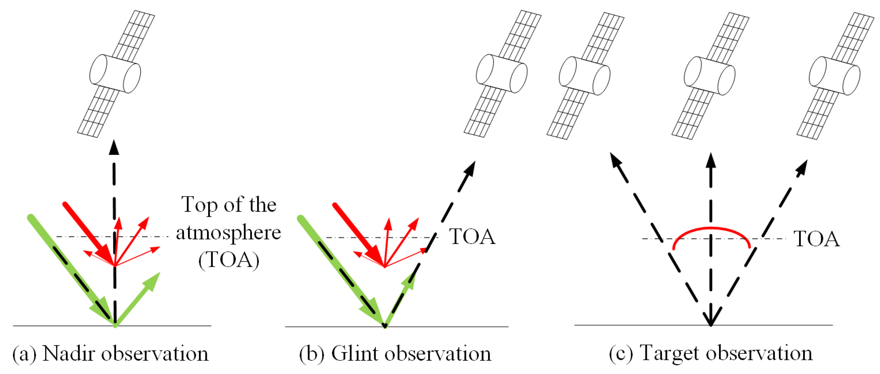
Figure 3.
The observation modes of GAS-2. (a) Nadir observation mode; (b) glint observation mode; (c) target observation mode.
Figure 3.
The observation modes of GAS-2. (a) Nadir observation mode; (b) glint observation mode; (c) target observation mode.
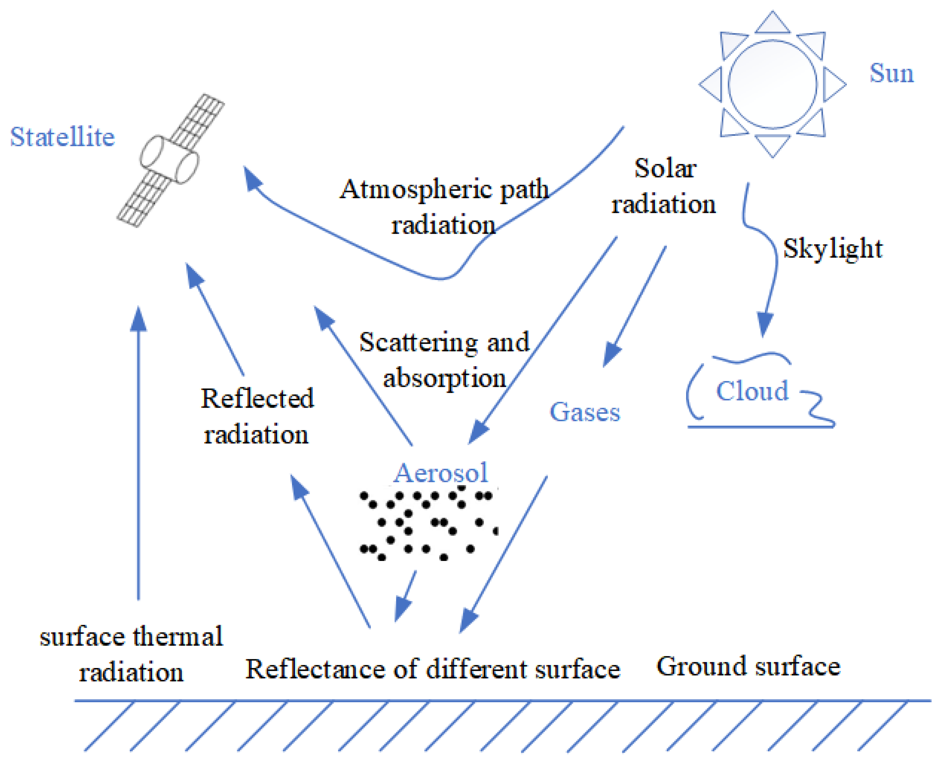
Figure 4.
Schematic diagram of remote sensor in environmental radiation.
Figure 4.
Schematic diagram of remote sensor in environmental radiation.
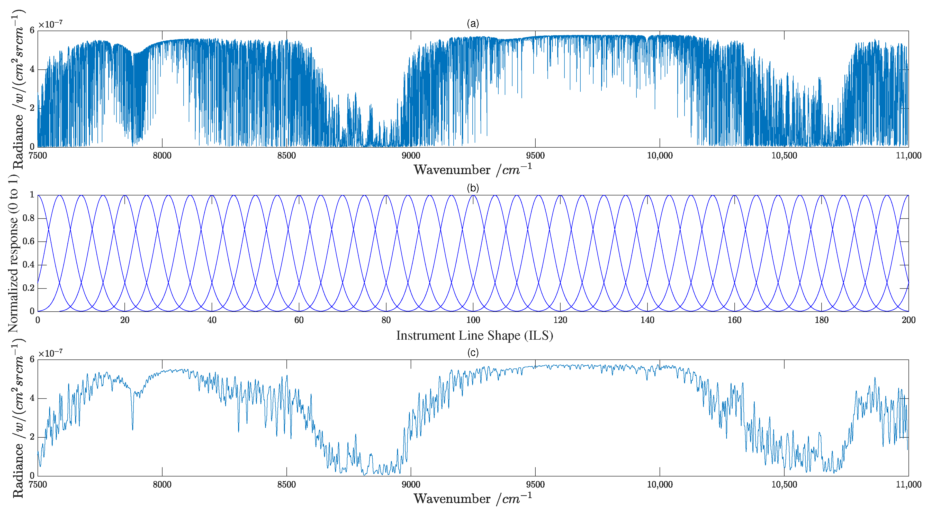
Figure 5.
Schematic representation of the convolution of the upwelling radiance spectrum with the instrument line shape (ILS). (a) The upwelling radiance spectrum obtained with MODTRAN5.2.1; (b) The instrumental line shape (ILS) function of the spectral channel; (c) Spectral radiance acquired by the instrument, which is the convolution of (a,b).
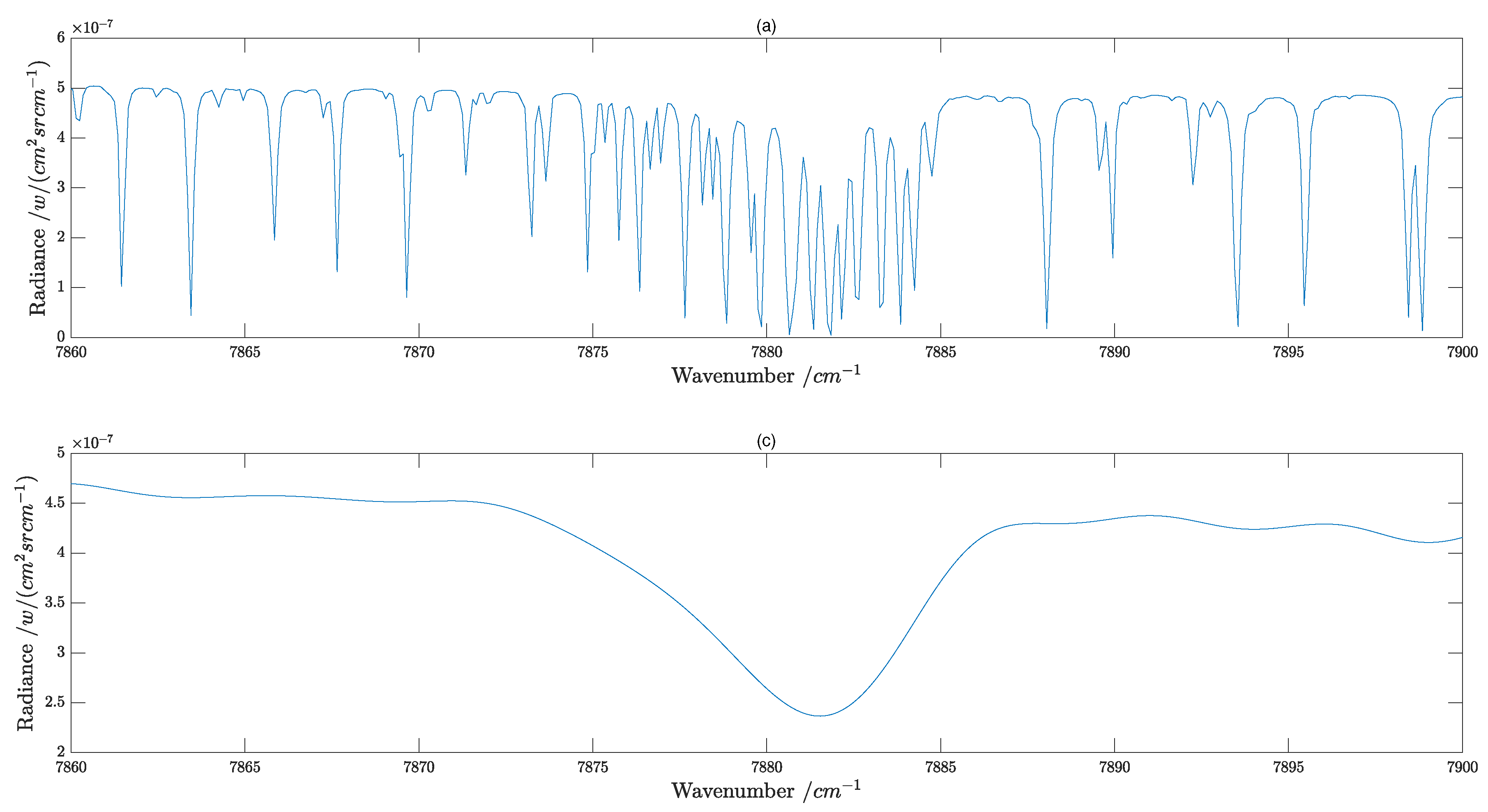
Figure 6.
The local magnification of (
a) and (
c) in
Figure 5; the wavenumber range is from 7860 cm
to 7960 cm
, and (
a) and (
c) in
Figure 6 correspond one-to-one to (
a) and (
c) in
Figure 5. (
a) The upwelling radiance spectrum obtained with MODTRAN 5.2.1. (
c) Spectral radiance acquired by the instrument, which is the convolution of (
a) and ILS (Gaussian function).
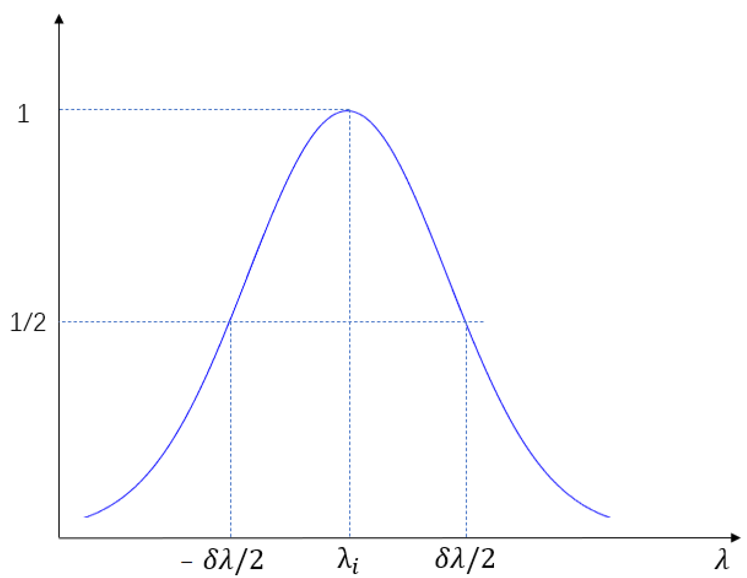
Figure 7.
Spectral response function of hyperspectral imaging spectrometer.
Figure 7.
Spectral response function of hyperspectral imaging spectrometer.
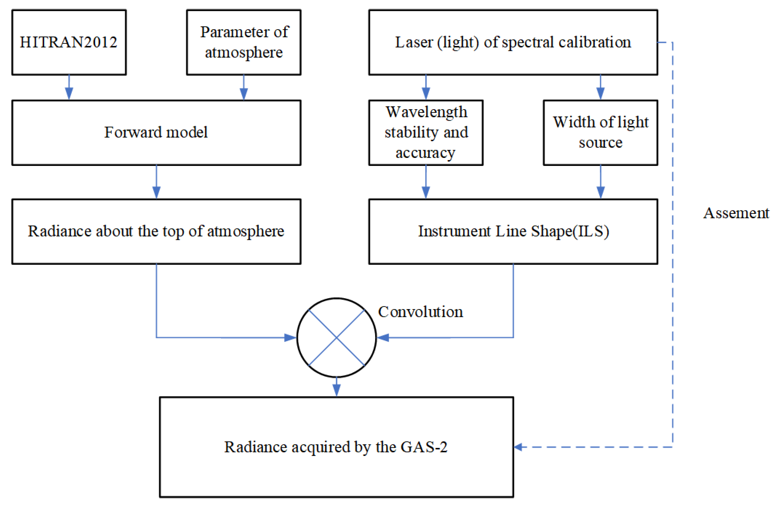
Figure 8.
Flowchart for assessing the effect of spectral calibration light source on the spectral radiance obtained via GAS-2.
Figure 8.
Flowchart for assessing the effect of spectral calibration light source on the spectral radiance obtained via GAS-2.
Figure 9.
Simulation results of spectral resolution error caused by linewidth of the calibration light source.
Figure 9.
Simulation results of spectral resolution error caused by linewidth of the calibration light source.
Figure 10.
Comparison of the spectral radiance of the FWHM error obtained from calibration sources with different linewidths. (a) The spectral radiance obtained via GAS-2 in the -A band with FWHM errors of 1%, 5%, 10%, 30%, and 60% due to calibration light source’s linewidth, respectively; (b) the spectral radiance obtained via GAS-2 in the weak- band with FWHM errors of 1%, 5%, 10%, 30%, and 60% due to calibration light source’s linewidth, respectively; (c) the spectral radiance obtained via GAS-2 in the strong- band with FWHM errors of 1%, 5%, 10%, 30%, and 60% due tocalibration light source’s linewidth, respectively; (d) the spectral radiance obtained via GAS-2 in the band with FWHM errors of 1%, 5%, 10%, 30%, and 60% due to calibration light source’s linewidth, respectively.
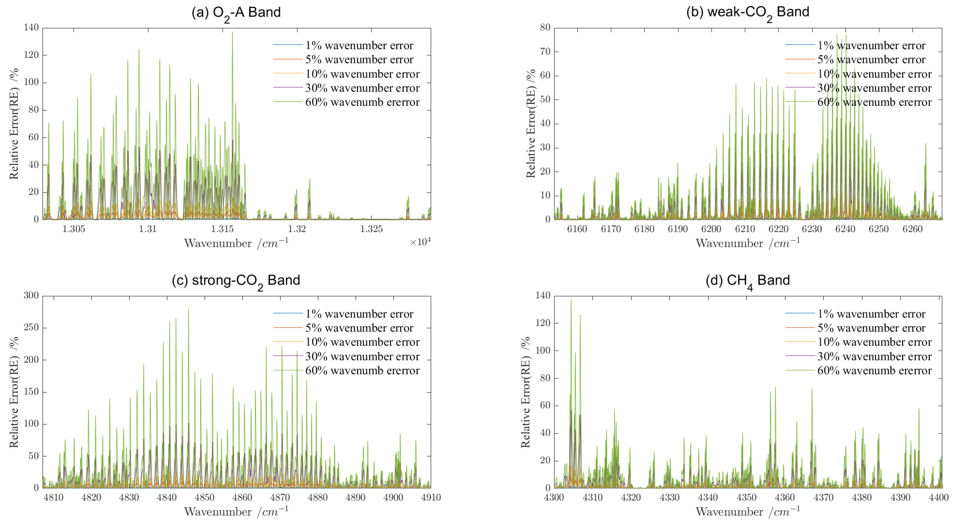
Figure 11.
Comparison of relative error (RE) of spectral radiance obtained via GAS-2 in four bands with different FWHM errors of 1%, 5%, 10%, 30%, and 60%. (a) -A band, the relative error (RE) of spectral radiance; (b) weak- band, the relative error (RE) of spectral radiance; (c) strong- band, the relative error(RE) of spectral radiance; (d) band, the relative error (RE) of spectral radiance.
Figure 12.
Comparison of relative error (RE) of spectral radiance acquired via GAS-2 due to 1%, 5%, 10%, 30%, 60% shift in center wavelength. (a) -A band, the relative error (RE) of spectral radiance due to central wavelength shift; (b) weak- band, the relative error (RE) of spectral radiance due to central wavelength shift; (c) strong- band, the relative error (RE) of spectral radiance due to central wavelength shift; (d) band, the relative error (RE) of spectral radiance due to central wavelength shift.
Figure 13.
Comparison of relative error (RE) of spectral radiance acquired via GAS-2 in four bands due to 1%, 5%, 10%, 30%, 60% shift in center wavelength and 1%, 5%, 10%, 30%, 60% spectral resolution (FWHM) error in -A band. (a) -A band, relative error (RE) of spectral radiance due to different wavelength errors when the FWHM error is 1%; (b) -A band, relative error (RE) of spectral radiance due to different wavelength errors when the FWHM error is 5%; (c) -A band, relative error (RE) of spectral radiance due to different wavelength errors when the FWHM error is 10%; (d) -A band, relative error (RE) of spectral radiance due to different wavelength errors when the FWHM error is 30%; (e) -A band, relative error (RE) of spectral radiance due to different wavelength errors when the FWHM error is 60%.
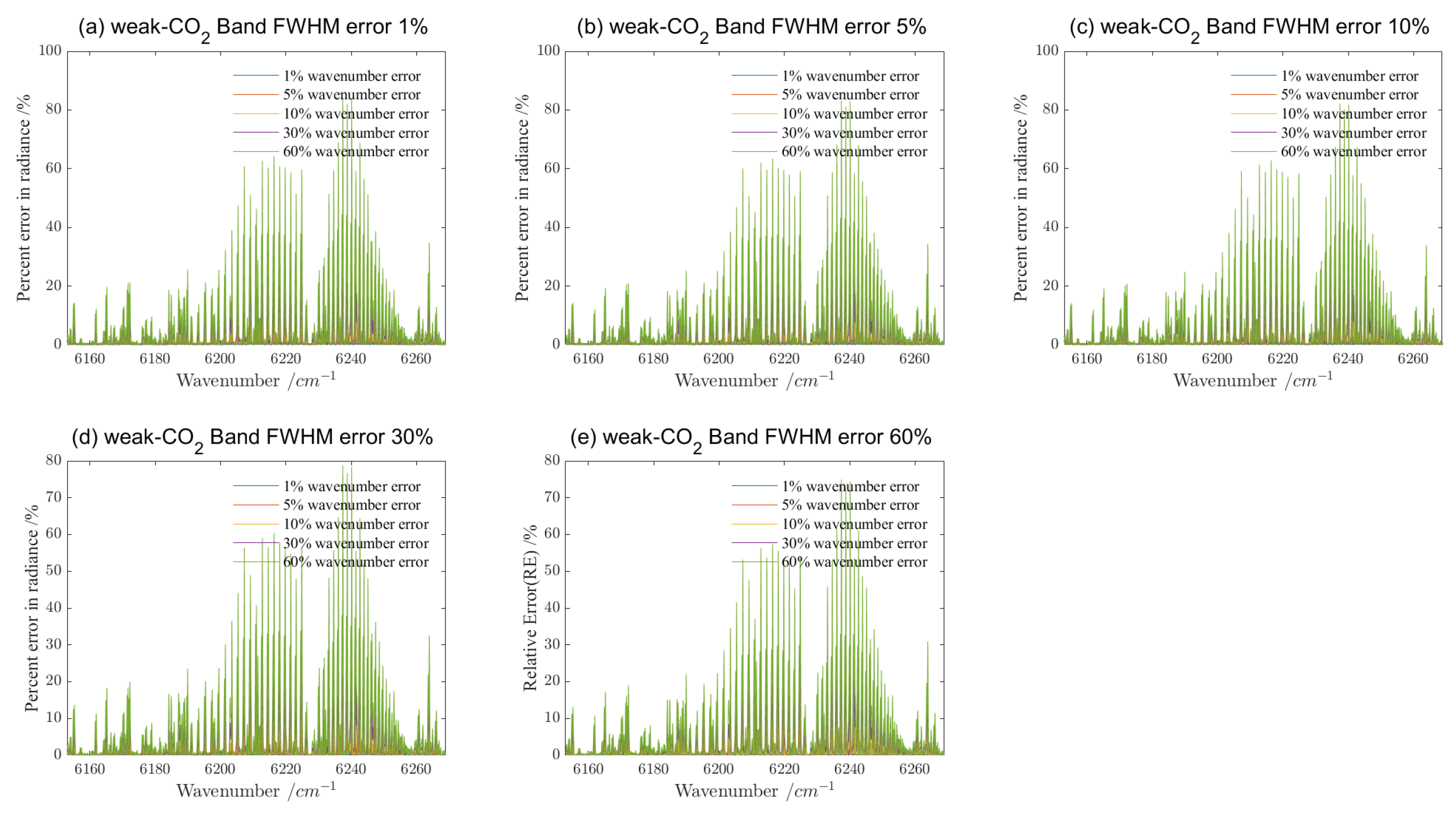
Figure 14.
Comparison of relative error (RE) of spectral radiance acquired via GAS-2 in four bands due to 1%, 5%, 10%, 30%, 60% shift in center wavelength and 1%, 5%, 10%, 30%, 60% spectral resolution (FWHM) error in weak- band. (a) weak- band, relative error (RE) of spectral radiance due to different wavelength error when the FWHM error is 1%; (b) weak- band, relative Error (RE) of spectral radiance due to different wavelength error when the FWHM error is 5%; (c) weak- band, relative error (RE) of spectral radiance due to different wavelength error when the FWHM error is 10%; (d) weak- band, relative error (RE) of spectral radiance due to different wavelength error when the FWHM error is 30%; (e) weak- band, relative error (RE) of spectral radiance due to different wavelength error when the FWHM error is 60%.
Figure 15.
Comparison of relative error (RE) of spectral radiance acquired via GAS-2 in four bands due to 1%, 5%, 10%, 30%, 60% shift in center wavelength and 1%, 5%, 10%, 30%, 60% spectral resolution (FWHM) error in strong- band. (a) strong- band, relative error (RE) of spectral radiance due to different wavelength error when the FWHM error is 1%; (b) strong- band, relative error (RE) of spectral radiance due to different wavelength error when the FWHM error is 5%; (c) strong- band, relative error (RE) of spectral radiance due to different wavelength error when the FWHM error is 10%; (d) strong- band, relative error (RE) of spectral radiance due to different wavelength error when the FWHM error is 30%; (e) strong- band, relative error (RE) of spectral radiance due to different wavelength error when the FWHM error is 60%.
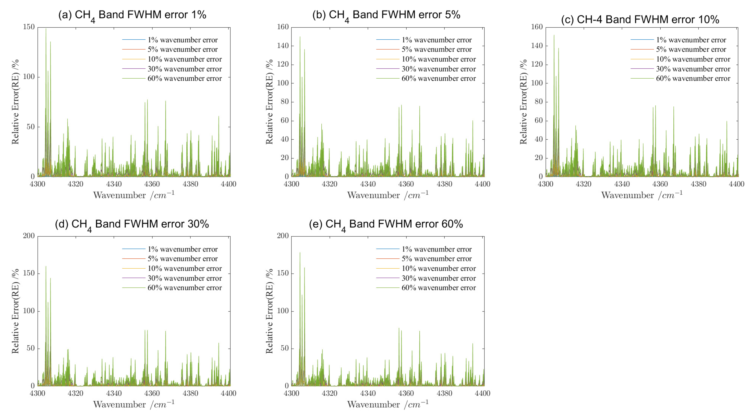
Figure 16.
Comparison of relative error (RE) of spectral radiance acquired via GAS-2 in four bands due to 1%, 5%, 10%, 30%, 60% shift in center wavelength and 1%, 5%, 10%, 30%, 60% spectral resolution (FWHM) error in band. (a) band, relative error (RE) of spectral radiance due to different wavelength error when the FWHM error is 1%; (b) band, relative error (RE) of spectral radiance due to different wavelength error when the FWHM error is 5%; (c) band, relative error (RE) of spectral radiance due to different wavelength error when the FWHM error is 10%; (d) band, relative error (RE) of spectral radiance due to different wavelength error when the FWHM error is 30%; (e) band, relative error (RE) of spectral radiance due to different wavelength error when the FWHM error is 60%.
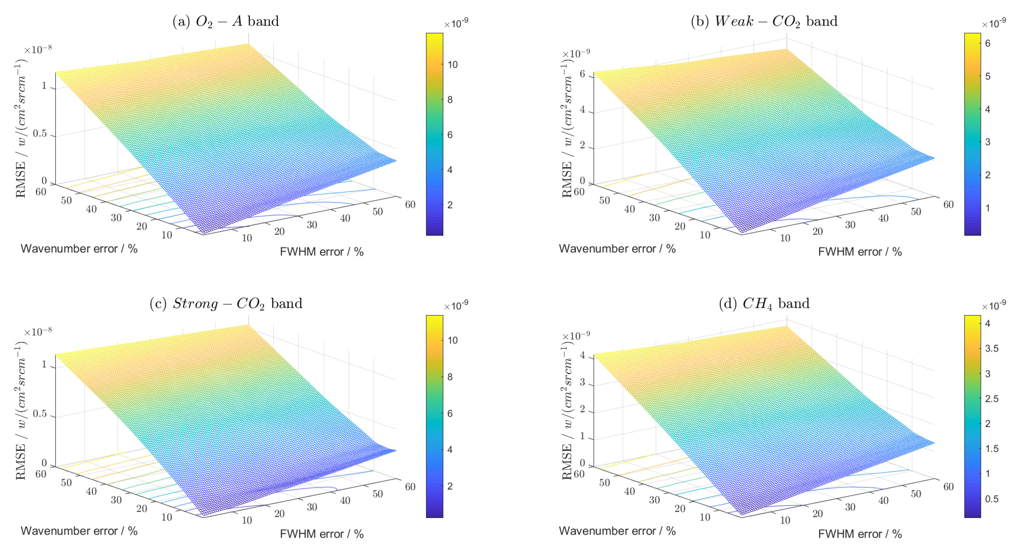
Figure 17.
Comparison of RMSE results of spectral radiance acquired via GAS-2 in four bands due to wavelength stability and linewidth of the calibration light source. (a) -A band, the RMSE results of spectral radiance due to two factors operating simultaneously; (b) weak- band, the RMSE results of spectral radiance due to two factors operating simultaneously; (c) strong- band, the RMSE results of spectral radiance due to two factors operating simultaneously; (d) band, the RMSE results of spectral radiance due to two factors operating simultaneously.
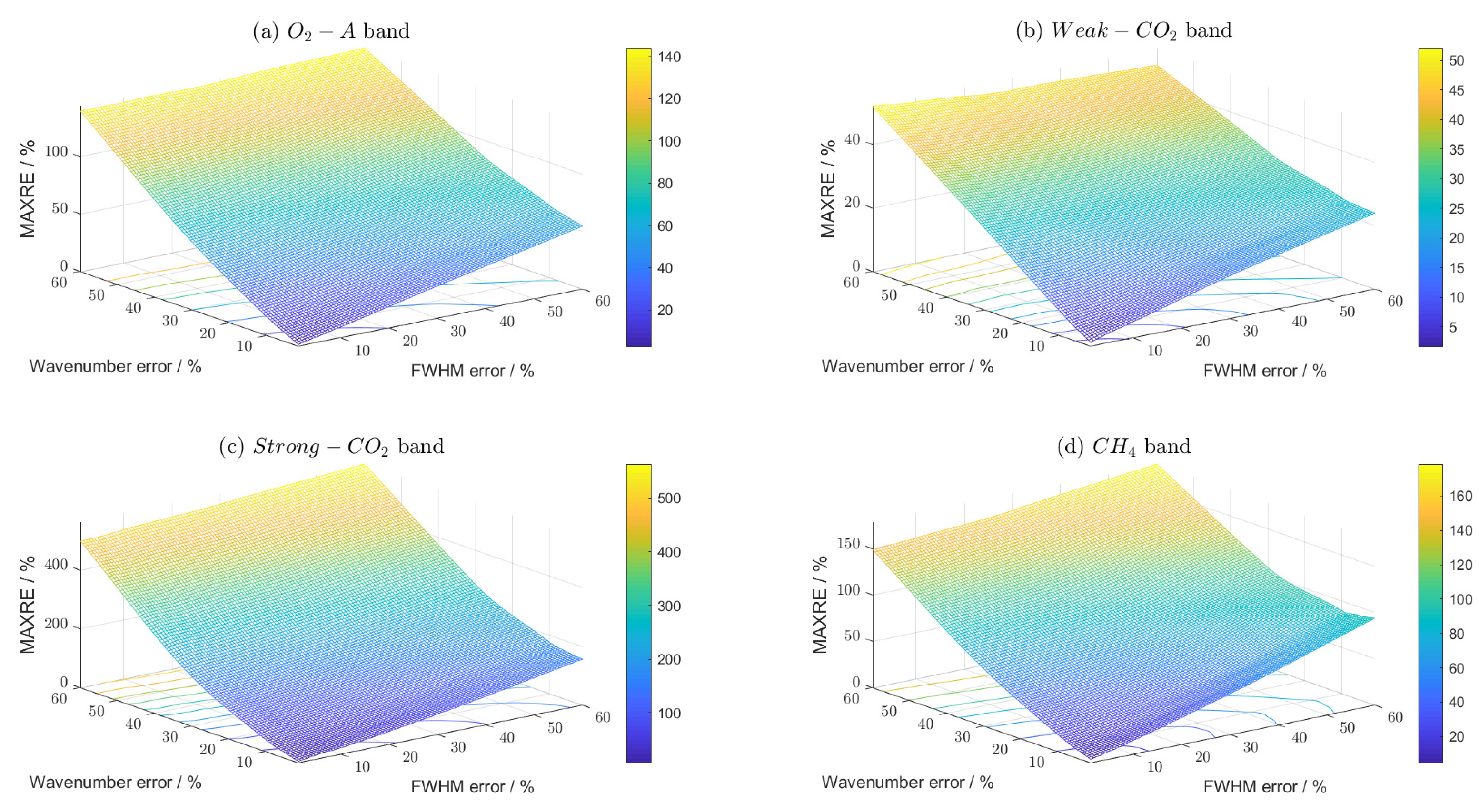
Figure 18.
Comparison of RE results of spectral radiance acquired via GAS-2 in four bands due to wavelength stability and linewidth of the calibration light source. (a) -A band, the RE results of spectral radiance due to two factors operating simultaneously; (b) weak- band, the RE results of spectral radiance due to two factors operating simultaneously; (c) strong- band, the RE results of spectral radiance due to two factors operatimg simultaneously; (d) band, the RE results of spectral radiance due to two factors operating simultaneously.
Figure 19.
Comparison of AE results of spectral radiance acquired via GAS-2 in four bands due to wavelength stability and linewidth of the calibration light source. (a) -A band, the AE results of spectral radiance due to two factors operating simultaneously; (b) weak- band, the AE results of spectral radiance due to two factors operating simultaneously; (c) strong- band, the AE results of spectral radiance due to two factors operating simultaneously; (d) band, the AE results of spectral radiance due to two factors operating simultaneously.
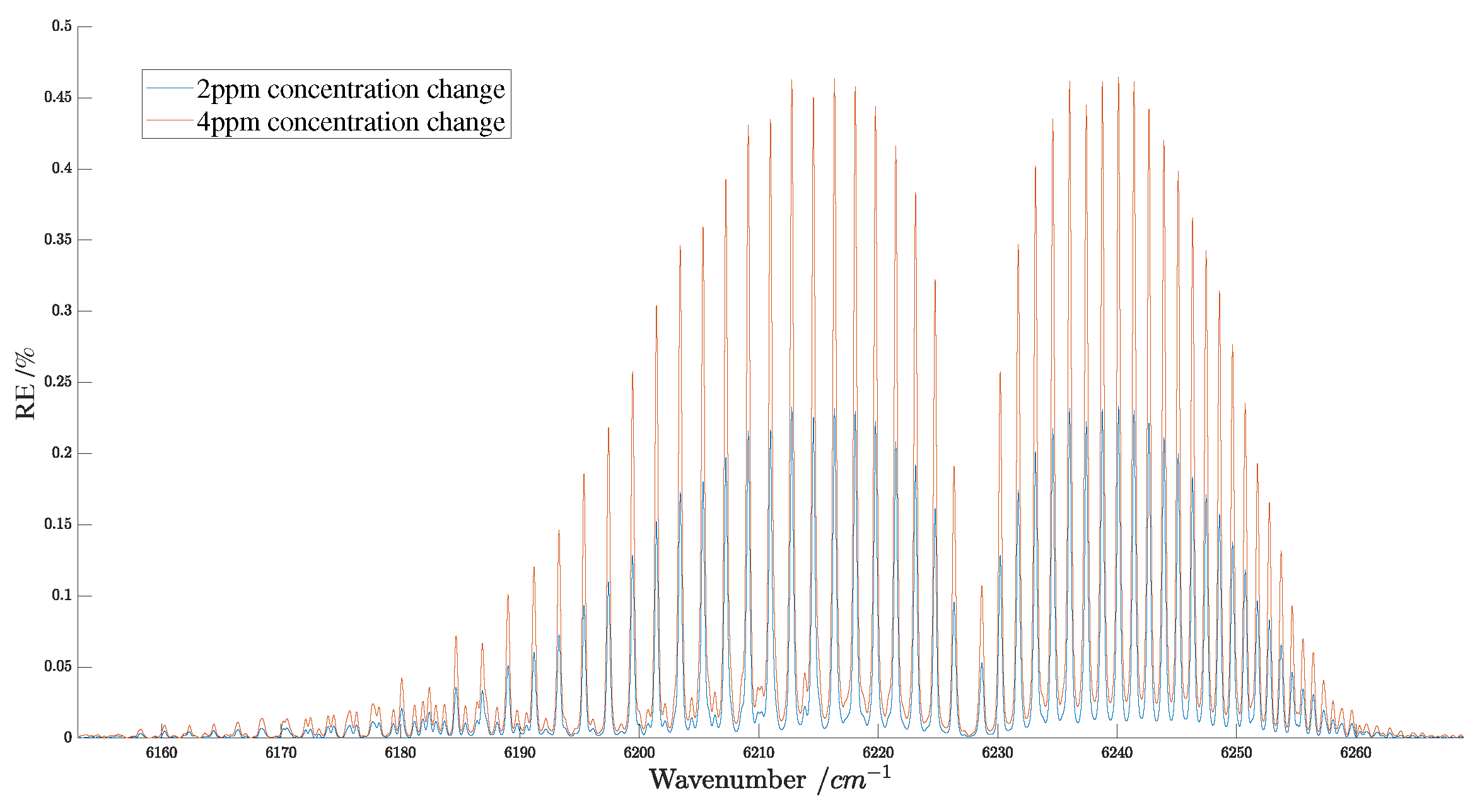
Figure 20.
Relative error in spectral radiance for 2 ppm and 4 ppm changes in atmospheric concentration.
Figure 20.
Relative error in spectral radiance for 2 ppm and 4 ppm changes in atmospheric concentration.
Table 1.
Main parameters of Greenhouse-gases Absorption Spectrometer-2 (GAS-2).
Table 1.
Main parameters of Greenhouse-gases Absorption Spectrometer-2 (GAS-2).
| Band | B1(-A) | B2(Weak-) | B3(Strong-) | B4() |
|---|
| Target | aerosol, surface pressure, , SIF | | | |
| Central wavelength (m) | 0.76 | 1.61 | 2.06 | 2.3 |
| Spectral range (m) | 0.7525–0.7675 | 1.595–1.625 | 2.04–2.08 | 2.275–2.325 |
| Spectral resolution (nm) | 0.04 | 0.07 | 0.09 | 0.1 |
| Observation mode | nadir observation, sunglint observation, target observation |
Table 2.
LBLRTM parameters set during simulation.
Table 2.
LBLRTM parameters set during simulation.
| Atmospheric Profile Model | 1976 US Standard Atmosphere |
|---|
| Spectral range | 13,029–13,290 cm, 6153–6270 cm, 480–4902 cm, 4301–4401 cm |
| Spectral resolution | 0.69 cm, 0.27 cm, 0.21 cm, 0.19 cm |
| mixing ratio | 400 ppm |
| Surface albedo | 0.05 |
| Observer zenith angle | 180° (Looking down vertically) |
| Solar zenith angle | 30° |
| Cloud/rain | No clouds or rain |
| Observer height | 100 Km |
| Slit function type | Gaussian |


