Article

CRSNet: Cloud and Cloud Shadow Refinement Segmentation Networks for Remote Sensing Imagery

1
Collaborative Innovation Center on Atmospheric Environment and Equipment Technology, Nanjing University of Information Science and Technology, Nanjing 210044, China
2
College of Information Science and Technology, Nanjing Forestry University, Nanjing 210000, China
*
Author to whom correspondence should be addressed.
Remote Sens. 2023, 15(6), 1664; https://doi.org/10.3390/rs15061664
Submission received: 15 February 2023 / Revised: 7 March 2023 / Accepted: 10 March 2023 / Published: 20 March 2023

Abstract

:
Cloud detection is a critical task in remote sensing image tasks. Due to the influence of ground objects and other noises, the traditional detection methods are prone to miss or false detection and rough edge segmentation in the detection process. To avoid the defects of traditional methods, Cloud and Cloud Shadow Refinement Segmentation Networks are proposed in this paper. The network can correctly and efficiently detect smaller clouds and obtain finer edges. The model takes ResNet-18 as the backbone to extract features at different levels, and the Multi-scale Global Attention Module is used to strengthen the channel and spatial information to improve the accuracy of detection. The Strip Pyramid Channel Attention Module is used to learn spatial information at multiple scales to detect small clouds better. Finally, the high-dimensional feature and low-dimensional feature are fused by the Hierarchical Feature Aggregation Module, and the final segmentation effect is obtained by up-sampling layer by layer. The proposed model attains excellent results compared to methods with classic or special cloud segmentation tasks on Cloud and Cloud Shadow Dataset and the public dataset CSWV.

1. Introduction

With the progress of remote sensing technology, it is commonly used in military, agricultural, meteorological and many indispensable areas of society. In remote sensing images, all ground targets may be covered by clouds, or located in cloud shadows, resulting in lower brightness and visibility than real [1]. This has affected our exploration of real ground targets, so the recognition and segmentation of clouds and shadows in remote sensing images is a question of great practical significance.
According to the existing practical use methods and the related literature, several common methods for cloud detection can be summarized: texture spectrum detection method based on spatial characteristics, artificial threshold method based on different bands, and detection method based on machine learning. The original method sets the threshold manually, Rossow and Schiffer [2] compared the radiation values of visible and infrared bands in the image, and tested the radiation values of pixels. When the radiation value was greater than that of the ground without cloud cover, it indicated that the radiation value of the region came from the cloud. Ackerman et al. [3] compared the thresholds of different spectral bands and obtained the preliminary detection results. They applied this method to MODIS data, and the experiment proved that this method was superior to the previous physical threshold detection method. Solvsteen et al. [4] studied the texture spectrum detection method of spatial features on cloud detection datasets based on ocean background. Adrian [5] Use thresholds to detect marker points, and segment clouds and shadows from marker points by watermark transform. The threshold method and feature texture detection method are traditional detection methods. The traditional method is sensitive to the threshold, which requires complex artificial steps and prior knowledge, and is susceptible to noise interference in remote sensing images. When thin clouds appear in the image or complex high-frequency noises appear on the ground, it is prone to cause misdetection or false detection.
In recent years, machine learning algorithms for remote sensing images such as SVM [6], sparse sensing [7], automatic encoder and decoder [8] are proposed to cloud detection tasks. Luis et al. [9,10] detected thin clouds and clouds overlapping the snow background by proposing an unsupervised clustering cloud detection algorithm. The clustering algorithm which proposed by Zhang et al. [11] is used for pixels on the remote sensing images, then segments these pixels by a hierarchical support vector machine. Pixels were divided into ‘thick cloud’, ‘thin cloud’ and ‘ground objects’. Liu et al. [12] proposed daytime and nighttime cloud detection algorithms, which vary depending on whether solar band observation is included, and compared them using artificial neural network (ANN) and random forest (RF) technology. Chen et al. [13] developed a new, threshold-free cloud mask algorithm based on a neural network classifier driven by extensive radiative transfer simulations, this method does not rely on thresholds and needs fewer satellite channels. The classical machine learning method has achieved certain accuracy in cloud detection, but they have some shortcomings that are difficult to solve the labeling and algorithm of cloud detection tasks by ML method need to be designed according to different factors, including but not limited to a season, landform, sensor type, etc. The classical machine learning method has achieved certain accuracy in cloud detection, but the detection results of high-resolution remote sensing images with rich details and remote sensing images with complex backgrounds are not ideal.
Due to its universality and good performance, deep learning is used in cloud detection more and more widely [14,15,16]. Deep learning can autonomously learn the features in the image [17,18,19,20,21]. Compared with the traditional method, it can achieve higher accuracy and greatly reduce the dependence on manual annotation. Long et al. [22] proposed the FCN, which uses a convolution layer rather than a full connection layer to classify at the pixel level. Chen et al. [23] proposed the Deeplab which expands the receptive field by dilated convolution. Zhao et al. [24] proposed PSPNet which can extract context information on different scales effectively to enhance the ability to learn global information. Chen et al. [25] proposed the MFANet algorithm to reduce the loss of detail and edge blur caused by subsampling. Qu et al. [15] proposed CSAMNet, which uses channel space attention and strip pooling to improve overall segmentation accuracy and optimize edge details. Zhang et al. [26] proposed that CDUNet used multi-scale convolution and spatial priority self-attention mechanisms to refine boundaries and strengthen fine cloud detection. Multi-scale strip feature fusion network proposed by Lu et al. [16] used improved pyramid pooling to extract multi-scale information and fused both high-level and low-level semantics to obtain higher segmentation results.
Even though the deep learning method can complete most semantic segmentation tasks well, the effect is not perfect for cloud and shadow segmentation tasks [27]. Firstly, the overall accuracy of recognition needs to be improved, and the boundary between cloud and shadow is not fine enough. Secondly, background noise has always been a big problem, such as large white houses on the ground and low-brightness rivers being easily classified as clouds or shadows. Finally, thin clouds and small-scale clouds and cloud shadows are often missed. To improve the predicted result on the cloud detection task, we propose the Cloud and Cloud Shadow Segmentation Network (CRSNet). CRSNet is composed of ResNet [28] proposed by He et al. in 2016 as the backbone. Multi-scale Global Attention Module (MGA), Strip Pyramid Channel Attention Module (SPCA) and Hierarchical Feature Aggregation Module(HFA). This model uses ResNet-18 as the backbone. The fitting residual mapping introduced by ResNet can well solve the problems of gradient disappearance and gradient explosion in deep networks, and can better extract the features at different levels. In the process of feature extraction, the attention of space and channel is strengthened through the MGA module for each layer of features to improve the accurate segmentation ability. Meanwhile, the subsampling characteristics of each layer through MGA are further studied by the SPCA module to learn multi-scale spatial information independently and establish the cross-channel interaction in a local way to enhance the detection ability of clouds with different scales. Finally, upsampling the feature by HFA, to make the high-dimensional features and low-dimensional features fused layer by layer. Meanwhile, it strengthens the context connection of each layer of features, making the spatial information retained by shallow features and the rich semantic information of deep features guide each other.
The following part of this paper will introduce the method proposed in this paper, as well as the analysis and results of ablation experiments, comparative experiments, and generalization experiments, and finally, give the conclusion.

2. Methodology

Figure 1 shows the structure of the model.CRSNet is composed of a resnet backbone, Multi-scale Global Attention Module, Strip Pyramid Channel Attention Module and Hierarchical Feature Aggregation Module. It improves the encoder and decoder structure, uses the attention module at the channel and spatial levels, and captures the long-distance dependency in space globally. Firstly, ResNet-18 is used for subsampling images with any size input to extract features at different levels. The extracted features of each layer are enhanced by the MGA module to enhance the spatial and channel attention of the model to the image. The processed features are then processed by SPCA to learn spatial information on a multi-scale to enhance the detection of fine clouds and shadows. In the decoding process, we propose the HFA module, which combines the rich semantic information in deep features and spatial information in shadow features to achieve a better boundary segmentation effect while strengthening the feature self-attention.

2.1. Backbone

ResNet is an architecture for deep convolutional neural networks proposed by He et al. in 2016. It adopts the idea of residual learning, making the network easier to train and enabling the training of deeper networks than before. In traditional convolutional neural networks, each layer output is obtained through a series of convolutions and nonlinear transformations. However, as the network depth increases, problems such as vanishing or exploding gradients become more severe, making model training difficult. The idea of residual learning is to solve this problem by introducing “residual blocks”, so that each layer output depends not only on the input of that layer but also on the difference between the output and the input of that layer, making the network easier to train. It also provides structures with different depths and widths to obtain appropriate networks according to tasks. We chose resnet18 to extract image features because it has appropriate parameter quantity and sufficient performance. The original ResNet is used for classification, we removed its classification output and only took its subsampling part.

2.2. SPCA

Semantic information is gradually lost during feature subsampling, so it is very important for deep neural networks to capture long-distance correlation [29,30]. However, the receptive field of convolution is limited, and it is hard to capture the remote correlation of features [31]. To improve the semantic information of deep features, it is necessary to increase the receptive field. Except for using dilation convolution [32], the pyramid structure proposed by Zhao et al. [24] is another way to increase global information. In the past models involving pyramid structure, pooling is often used to obtain the feature information at different scales, but pooling is very serious for the loss of details, which leads to the pooling pyramid model being only effective for the identification of large-scale targets in the cloud detection task, and does not help the detection effect of small clouds and shadows. To make up for this deficiency, we propose to use strip convolution [33] to extract features from different scales. There are three advantages of using strip convolution to extract features. Firstly, using convolution instead of pooling for subsampling can reduce the loss of information [34]. Secondly, strip convolution deploys a long strip pooled kernel shape along a spatial dimension, so it can capture the long-distance relationship of isolated regions [33]. Moreover, the strip convolution maintains a narrow kernel shape in spatial dimensions, it is convenient for capturing local context and preventing irrelevant regions from interfering with prediction. Thirdly, with the increase of convolution kernel size in the pyramid structure, the number of parameters is also significantly increased, and the strip convolution module can reduce the consumption of memory.
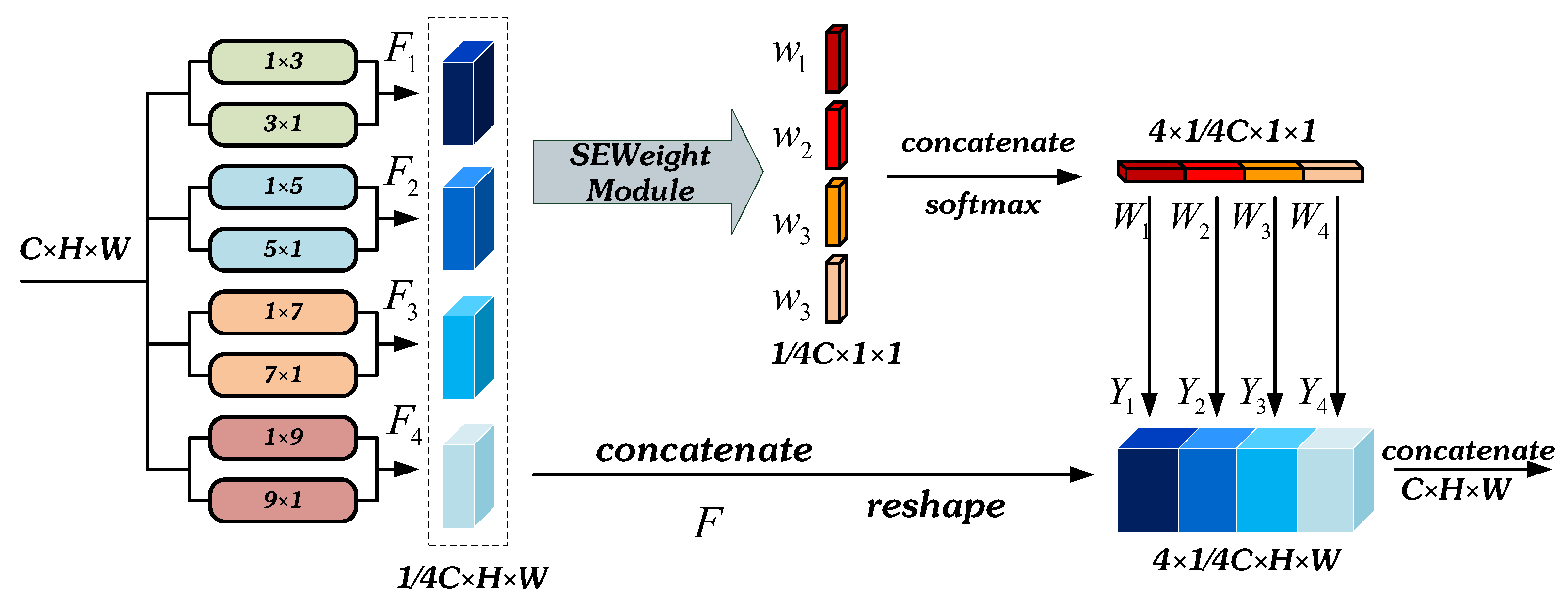
Channel attention mechanism allows the network to adapt to the weight of each channel, thus generating more representative features. SE module [35] is a simple and effective module, it uses Squeeze–Excitation to extract the weight of channels, it is simple and efficient. Therefore, after obtaining the features at different scales, we let each feature block pass through the Squeeze–Excitation weight (SEWeight) module to obtain their respective channel weight vectors, and then multiply the corresponding features by Softmax [36], so that each feature block independently learns multi-scale spatial information. SEWeight module consists of compression and incentive. The squeezing part can encode global information, and the excitation part can adaptively obtain the importance weights between channels. We embed global spatial information into channel information by global averaging pooling. The structure of SEWeight is shown in Figure 2. The process of the SEWeight module can be mathematically expressed as:
g c = G A P x c = 1 H × W i = 1 H j = 1 W x c i , j ,
W c = σ ( W 1 r ( W 0 ( g c ) ) ) ,
where G A P represents global average pooling, x c represents the input feature map. H and W represent the height and width of the feature map. r represents the R e L U [37] activation function. W 0 is a 1 × 1 convolution with input C and output C / r , W 1 is a 1 × 1 convolution with input C / r and output C. Two 1 × 1 convolutions replace fully connected operations that can effectively adapt to the relationship between learning channels with fewer parameters and enhance the nonlinearity of the model. Symbol σ denotes the activation function Sigmoid.
As shown in Figure 3, combined with the above two points, we propose the SPCA. Firstly, we use four strip convolutions with different kernel sizes to extract features of different scales to construct feature pyramids. Secondly, we use the SEWeight module to calculate the channel attention of different feature blocks. Third, Softmax acts on the channel attention vector to obtain the recalibration weight of multi-scale channels. Fourthly, the recalibrated weights and corresponding features are multiplied by corresponding elements. Finally, output the refined feature map of more abundant multi-scale feature information.
When constructing the feature pyramid with strip convolution, increasing the kernel size in parallel will make the number of parameters increase significantly. To make the best of multi-scale spatial location information without increasing the amount of computation, we use group convolution when extracting feature maps of different scales. As shown in Table 1, different grouping schemes have a significant impact on the results of the Cloud and Cloud Shadow dataset which is the main dataset we used in this paper. The improvement of packet convolution is not only in MIoU, by properly adjusting the group size, but the number of parameters and the computational cost can also be reduced by a factor that equals the number of sub-groups. By adjusting the size of the group, the optimal results can be obtained while reducing the computational cost. Then we splice the features of different scales in the channel dimension and recombine their dimensions to multiply the multi-scale channel attention obtained below. The process can be expressed as:
F i = S t r i p C o n v ( k i , G i ) , F i R C / 4 × H × W , i = 0 , 1 , 2 , 3 ,
F = C a t ( F 0 , F 1 , F 2 , F 3 ) ,
F R C × H × W F R 4 × C / 4 × H × W ,
where k i and G i represent the size of the strip convolution kernel. Cat indicates the splicing operation in the channel dimension. Different scale features are passed through the SEWeight to obtain channel attention weight vectors of different scales:
w i = S E W e i g h t ( F i ) , w i R C / 4 × 1 × 1 , i = 0 , 1 , 2 , 3 .
We spliced the channel attention vectors of different scales in the channel dimension. Then we recombine the dimensions of the obtained multi-scale channel attention vector to further realize the interaction of channel attention:
W i = S o f t max ( w i ) , W i R C / 4 × H × W , i = 0 , 1 , 2 , 3 .
After obtaining the multi-scale channel weight Wi, we multiply it with the corresponding elements of different scale features on the corresponding channel and splice it in the channel dimension as output. This process can be expressed mathematically as follows:
Y i = F i W i ,
O u t = C a t ( [ Y 0 , Y 1 , Y 2 , Y 3 ] ) , O u t R C × H × W ,
where ∗ represents the corresponding multiplication in the channel dimension.
Through the attention module of the strip pyramid channel, we can have a larger receptive field and detect clouds and cloud shadows in finer granularity. At the same time, the multi-scale channel attention obtained by local and global interaction can make the model make better use of the global semantic information, and improve the detection accuracy and anti-noise ability.

2.3. MGA

In order to get a better segmentation effect, we should focus on both spatial information and semantic information. Shallow features have high resolution and contain a lot of spatial information. With continuous sampling, the feature size becomes smaller, the spatial information gradually disappears, and the semantic information increases. Both of them are important to the results of segmentation tasks. Channel attention only focuses on the category information, and spatial attention focuses on the location information of the segmentation target. To better extract the category and location of clouds and strengthen the weight distribution of features, we added two attention mechanisms in this module. It can make the whole module focus on clouds and cloud shadows, suppress irrelevant noise on the ground, make the model pay attention to the context of the important region adaptively, and make the segmentation result have finer boundaries while improving the segmentation accuracy.
SENet [35] can capture channel correlation by selectively modulating the channel scale, but only focuses on the semantic information on the channel, ignoring the spatial location information. CBAM [38] can enhance attention in the channel and spatial dimensions. Inspired by CBAM, GSoP-Net [39] proposed a second-order pool method to extract more abundant feature aggregation. Fcanet [40] proposed a new multispectral channel attention and realized the preprocessing of channel attention mechanism in the frequency domain. GCNet [41] introduces a simple spatial attention module to develop a remote channel dependency. DANet [42] proposed the PAM and the CAM, which establish rich context correlation on local features and significantly improve the segmentation results. The performance of the attention mechanism in image tasks is getting better and better. However, there are still two critical problems to be solved. First, how to effectively capture and use the spatial information of different scale feature maps to enrich the element space. Second, due to the reduction and separation of information caused by global pooling and maximum pooling, these attention mechanisms can only accept limited receptive fields, so the spatial or channel attention can only capture local information, and lose the interaction of global spatial channels finally.
Therefore, we propose MGA, which is designed to avoid the defects of the attention method described above. This module is composed of a Hierarchical Multi-scale Convolution module(HMC), global spatial attention and global channel attention. In terms of the overall structure, HMC convolutes different channels of the feature vector with different scales, respectively, and iteratively adds and repeatedly convolutes the obtained results to obtain more comprehensive feature information. To decrease the loss of spatial information, the global spatial attention and the global channel attention both omit the pooling operation commonly used in the previous attention mechanism like CBAM. Global channel attention also avoids the traditional method of expanding the features into one dimension and fully connecting to obtain the channel dimension weight, so that the relationship between channels can be preserved more completely. The structure of MGA is shown in Figure 4.
In terms of implementation details, the relatively high-resolution shallow feature F L R C × H × W passes through HMC to obtain the feature F L H M C R 2 C × H / 2 × W / 2 that extracts rich spatial information of shallow features, and add it to the high-dimensional feature F H R 2 C × H / 2 × W / 2 output from the next layer backbone to obtain the preliminary feature F R 2 C × H / 2 × W / 2 , then uses the initial feature F to obtain the weight W S and W C by parallel global spatial and channel attention.
F = F L H M C + F H = H M C ( F L ) + F H ,
W C = P C × W × H H × W × C { M L P [ P W × H × C C × H × W ( F ) ] } ,
W S = σ { C o n v u p 7 × 7 [ C o n v d o w n 7 × 7 ( F ) ] } ,
where P represents permutation operation, which is used to adjust the dimension of the matrix, and M L P represents full connection operation in the channel dimension. Finally, W S and W C are multiplied by the initial feature F to obtain the feature M S and M C that enhance the spatial and channel attention of the target in the global range, and add the initial feature F C which after convolution to output F O R 2 C × W / 2 × H / 2 :
F O = ( W C + W S ) × ( F L H M C + F H ) + C ( F ) = ( W C + W S ) × F + F C = M C + M S + F C .
High-resolution features always have noise inevitably, so we need to filter the information in advance by convolution. The multi-scale feature is very necessary for many image tasks. We construct hierarchical connections to represent multi-scale features in a more fine-grained manner and increase the receptive field of each layer. In order to realize the above functions, we design HMC to filter the feature map before attention enhancement.
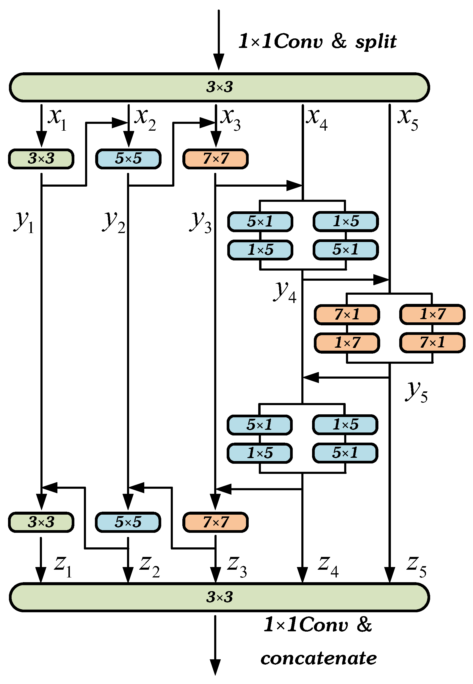
As shown in Figure 5, after adjusting the number of channels by 1 × 1 convolution, we divide features into s groups of feature subsets in the channel dimension through the split operation. The size of each feature subset is as same as the initial feature map, but channels are reduced to 1 / s of the original, expressed as x i , i { 1 , 2 , , s } . Except for the last group uses one convolution to extract features, the rest uses two convolutions. First, the output of the previous convolution and the next feature subset is added as the input of the next convolution. This process is repeated to the last group, and the output y i , then the output of the last group and the output of the previous group are added as the input of the second convolution layer of the previous group. This process is also repeated to the first group to obtain the output z i . The output of each layer can be expressed by the formula:
y i = C 1 i ( x i ) , i = 1 C 1 i ( x i + y i 1 ) , 1 < i s
z i = C 2 i ( z i + 1 + y i ) , 1 i < s y i , i = s
where C 1 i ( · ) represents convolutions of the first layer, C 2 i ( · ) represents convolutions of the second layer except the last path. s represents the number of groups. After the output z i is obtained, we merge z i in the channel dimension and adjust the number of channels to the number we want to output by 1 × 1 convolution.
In the ablation experiment, the MIoU of the model with the HMC module was 0.25% higher than the model without HMC. The results are shown in Table 2, and the details of the ablation experimental are shown in Section 3.3.

2.4. HFA

After extracting the category information in the encoding stage, we need to restore it to the original picture size layer by layer in the decoding stage to achieve the classification effect of pixel by pixel. During the process of subsampling, the image size is compressed, and the position information of the target is gradually lost. Upsampling by simple bilinear interpolation will get a result that has rough edges and low accuracy. We propose HFA to solve these problems. This module makes the category information of deep features participate in the upsampling of shallow features, which can enhance the classification effect while preserving the location information. At the same time, we pass the shallow features through the Improvement Self-attention Module (ISA). Non-local which was proposed by Wang et al. [43] uses the similarity of two points in the image to weigh the features of each position and can capture the correlation of two pixels with a long distance on the picture. Our improved self-attention module uses 3 × 3 convolutions to learn the context information to obtain the key, then concatenate the query and the context information after learning, and then use two consecutive 1 × 1 convolutions to extract local information. This operation can not only notice the relationship between independent pixels but also the semantics around the pixels so that it grasps the long-distance dependence between pixels at the global level to make shallow features have more accurate location information. We conducted relative ablation experiments. In the ablation experimental the MIoU of the model with ISA was 0.06% higher than that of the model without ISA. The results are shown in Table 2.
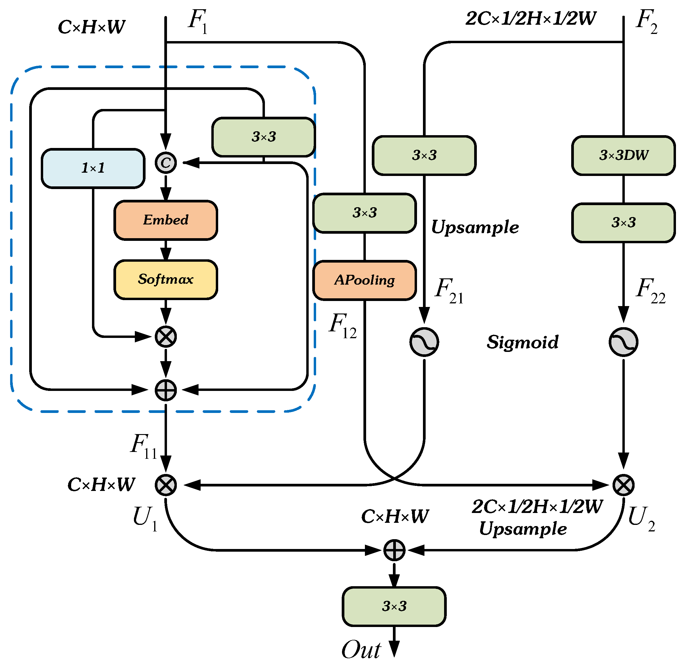
Figure 6 shows the structure of HFA. We let the shallow feature F 1 pass through the ISA to obtain the shallow feature F 1 1 with enhanced location information. Furthermore, let the deep feature F 2 pass through 3 × 3 convolution and bilinear interpolation upsampling to change its size to F 1 2 which is the same as the shallow layer feature, then weighted by sigmoid and the corresponding elements are multiplied with the shallow features to obtain the shallow features U 1 with enhanced classification ability. The shallow layer feature F 1 obtains F 1 2 with the same size as the deep layer feature through average pooling. Furthermore, F 1 2 multiply by the deep feature F 2 2 which through two 3 × 3 convolution and Sigmoid, so as to obtain the deep feature U 2 that enhances the spatial information. Finally, U 2 is upsampled by bilinear interpolation and multiplied by U 1 . The obtained result is sent to 3 × 3 convolution to complete the fusion of deep features and shallow features. The above process can be mathematically expressed as:
F 11 = a t t e n t i o n ( F 1 ) ,
F 12 = A v p o o l i n g { B N [ C o n v 3 × 3 ( F 2 ) ] } ,
F 21 = B N [ C o n v 3 × 3 ( F 2 ) ] ,
F 22 = B N { C o n v 3 × 3 [ D W C o n v 3 × 3 ( F 2 ) ] } ,
U 1 = F 11 × S i g m i o d ( F 21 ) ,
U 2 = F 12 × S i g m i o d ( F 22 ) ,
O u t = σ [ C o n v 3 × 3 ( U 1 + U 2 ) ] ,
where C o n v 3 × 3 represents 3 × 3 convolution, D W C o n v 3 × 3 represents depthwise separable convolution. We set a group of D W C o n v 3 × 3 equal to the number of channels of the deep feature. BN represents the operation of BatchNorm. Symbol σ represents the activation function R e L U .

3. Experimental Analysis

3.1. Datasets

3.1.1. Cloud and Cloud Shadow Dataset

The training samples are collected from Google Earth. It shows aerial photos, satellite photos and geographic information systems (GIS) corresponding to the real location of the earth’s surface on its 3D earth model. The resolution of photos on Google Earth is at least 100 m, and the resolution of images on the Chinese Mainland is usually 30 m. The altitude of view is 15 km. The samples that we use for training are collected by meteorological experts from Yunnan Guizhou Plateau, Yunnan Plateau, Yangtze River Delta and other regions. The pictures collected in these areas have five different ground backgrounds of the forest, water area, house, desert and field, which can verify the model with the good anti-noise ability and generalization ability. Because of the limitation of GPU video memory, photos cannot be trained in their original size. We changed the original 4800 × 2692 resolution high-resolution remote sensing image divided into 224 × 224 size picture. After the screening, we get 11,642 pictures, and we divide these into 9313 training data and 2329 test data. The ratio of training sets to validation sets was 8:2. We used pixels with three kinds of colors that represent three different categories to label the picture. The pixel colors are red, green and black. We use three different colors to represent different classification targets. The cloud, cloud shadow and background are red, green and black, respectively.

3.1.2. CSWV Dataset

The CSWV dataset is a high-resolution cloud snow dataset created by Zhang et al. [44]. It includes 27 images of clouds and snow collected in the Cordillera mountains of North America. The resolution in the dataset CSWV is 0.5–10 m. The image contains complex ground background, including forest, grassland, Lake area, bare ground, etc. There are many different types of clouds in the image, including cirrus, cirrus cumulus, altocumulus, cumulus and stratiform clouds. Furthermore, in the dataset, snow is composed of permanent snow, stable snow and discontinuous snow. The diversity of clouds and snow increases the difference in their shape, size, thickness, brightness and texture, making the data set more general and representative. Because of the limitation of the device’s video memory, we cut the picture to 256 × 256. The number of pictures in the training set is 2874, and the number of pictures in the test set is 324. Figure 7 shows some samples in the above two datasets.
The label of the dataset is manually marked. In the Cloud and Cloud Shadow dataset, black, red and green represent the ground, cloud and cloud shadow, respectively. In the CSWV dataset, black, purple and white represent the ground, cloud and snow, respectively. Each label has a fixed RGB value. The trained model can classify the original image at the pixel level. The RGB value of the classified pixel is the RGB value of the corresponding label.

3.2. Experiment Details

Optimization

We adopt the “ploy” learning rate strategy, l r n e w = l r i n i t i a l × [ 1 ( i t e r max i t e r ) p o w e r ] , set power as 0.9, and the initial learning rate as 0.0001. To achieve sufficient convergence and accuracy of comparison, maxiter is the maximum training times, and we set it as 300.
L o s s ( x , c l a s s ) = x [ c l a s s ] + log i e x [ i ]
where x is the predict picture of the model output, c l a s s is label. Because the Adam optimizer converges rapidly and stably, in the experiments involved in this paper, we use the Adam optimizer with β 1 = 0.9 and β 2 = 0.999. Our GPU for training is RTX 3060 with 12 G video memory. In all experiments in this paper, the batch size of the two datasets is 24 and 16, respectively. In this paper, pixel accuracy (PA), mean pixel accuracy (MPA) and mean intersection over union (MIoU) to evaluate the performance of this method in cloud and cloud shadow segmentation tasks. The calculation formula of PA, MPA and MIoU is as follows:
P A = i = 0 k p i j i = 0 k j = 0 k p i j
M P A = 1 k i = 0 k p i j j = 0 k p i j
M I o U = 1 k + 1 i = 0 k p i i j = 0 k p i j + j = 0 k p j i p i i

3.3. Ablation Experiment

To verify the effectiveness of each module, we added different modules for experiments. The experimental results are shown in Table 2. The symbol “_” indicates the module without the sub-module. We conducted ablation experiments in both Cloud and Cloud Shadow dataset and the CSWV dataset to verify the generalization of models and modules.

3.3.1. Ablation for SPCA

The feature pyramid extracted by strip convolution can not only enable the model to have a larger receptive field, and also detect small-scale clouds and shadows in a more fine-grained manner. At the same time, building global channel attention in different scale features can make the model more focused on the global semantic information and improve detection accuracy. The experiment shows that the SPCA can increase the MIoU of prediction results from 92.98% to 93.62%.

3.3.2. Ablation for HFA

We extract the long-distance relationship between pixels through the improved self-attention module so that the shallow features have more precise position information. Meanwhile, the deep features and the shallow features guide each other during the process of upsampling and make full use of the semantic information of the deep features and the location information of the shallow features to decode. The HFA module enables the image to have fine edges while being accurately classified after decoding. The experiment shows that the accuracy of the HFA module can be improved by 0.3% on the basis of the original 93.62%. This module has sub-module ISF, which can bring 0.06% improvement on the basis of 93.86% after adding.

3.3.3. Ablation for MGA

MGA uses hierarchical multi-scale convolution to increase the receptive field of input features to extract finer features. Furthermore, the global channel and spatial attention mechanism are adopted to effectively capture the attention of the global channels and pixels while reducing the information loss, and enhancing the classification ability. The experiment shows that the MGA module can improve MIoU by 0.51% to 94.43% on the basis of the first two modules. The module also has a sub-module HMC, which contributes 0.25% improvement.
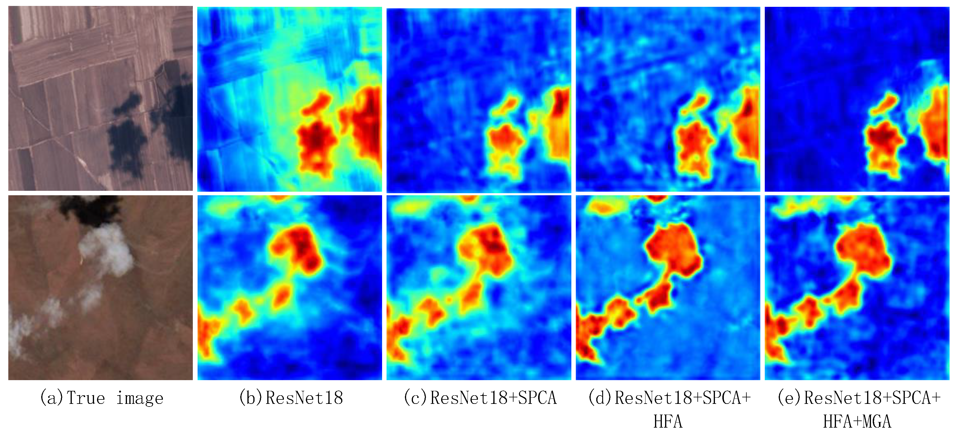
Figure 8 shows the heat map of attention composed of different modules. The first example is the degree of attention of the model to the cloud, and the second example is the degree of attention of the module to the cloud shadow. With the enrichment of modules, the model pays more and more attention to the detection target.

3.4. Comparison Test of the Cloud and Cloud Shadow Dataset

This experiment shows the performance of many existing excellent semantic segmentation models on Cloud and Cloud Shadow Datasets, such as UNet (2015) [45], DABNet (2019) [46], HRNet (2019) [47], OCRNet (2021) [48], ENet (2016) [49], ShuffleNetV2 (2018) [50], PSPNet (2021), SegNet (2017) [51] and Deeplabv3plus (2017) [52]. Furthermore, we also compared some networks specially designed for cloud detection tasks in recent years, such as Dual-branch Network (2022) [21], CSAMNet(2021) and PADANet (2021) [53]. The results of the experiment are shown in Table 3. The model with italics is designed specifically for the cloud detection task. Symbol “_” indicates no pre-training. The best result is bold, and the second-best result is underlined. Compared with other models, our CRSNet has the best performance, and the improvement on MIoU is at least 1.06% compared with other models.
As shown in Figure 9 and Figure 10, to show the advantage of CRSNet in cloud detection more intuitively, we compared the prediction pictures of the top 7 models in MIoU. CRSNet outperforms other models in dealing with this task. In the first sample, there are thin clouds in the area marked by the yellow square, which is almost ignored by ShuffleNetV2 and PSPNet, while other networks have different degrees of omission and misjudgment. Our model extracts the details of features with the help of HMC in the MGA module and strengthens the ability to extract semantic information through the integration of spatial and channel spatial attention. Therefore, it can also accurately detect thin clouds with less obvious characteristics. In the second sample, there is a white building next to a large area of white clouds, and the same color becomes the noise in the cloud detection process. Benefiting from the multi-scale strip convolution in the SPAC module to obtain multi-scale semantic information and strengthen the ability to judge the distance relationship in the image, it has a good ability to filter noise. In the third sample, the dark ground background is easy to be recognized as a cloud shadow. Almost all models have different degrees of misjudgment, but thanks to our model’s strong ability to extract semantic information, it can have a good segmentation effect on cloud shadow. In the fourth sample, there is a small cloud shadow in the marked box, which is easily ignored by the model. Only our model can correctly extract it. The strip pyramid and channel attention structure in the SPCA module of CRSNet proposed by us can well extract the long-distance dependence of targets and improve the detection ability of small targets. The HFA module takes advantage of ISA to simultaneously pay attention to the correlation between the independent pixels of the shallow features and the semantics around the pixels. It obtains the long-distance dependence between pixels at the global level, so it enables shallow features to have more accurate location information. Then, the classification information of deep features is used to guide the up-sampling of shallow features, and the classification effect is enhanced while the position information is retained.

3.5. Comparison Test of the CSWV

To further verify the generalization ability of the CRSNet, we also performed a generalization experiment on CSWV. The characteristics of the images in the CSWV dataset are that some thin clouds are easily confused with the bare ground, and some thicker clouds become brighter under the sunshine, which is easily confused with the snow. In addition, although snow is not the main target of our detection, it is usually clearly distinguished from the background, but it is hard for models to extract the snow edge accurately. The CRSNet performs very well in the above segmentation difficulties. We compared the predicted results of the CRSNet model with some classical models. The experimental results are shown in Table 4. The model with italics is designed specifically for the cloud detection task. Symbol “_” indicates no pre-training. The best result is bold, and the second-best result is underlined.
From the results, we can find that our performance on the CSWV dataset is the best. In the first sample, due to the obvious difference between the snow and the background, even though the snow area is small and the number is large, all models rarely miss detection. However, it is easy to see that the CRSNet has the finest segmentation edges. This is due to the excellent detail extraction capability of the multi-scale convolution module in CRSNet, which can finely segment the edges of the target. In the second sample, it is hard for the model to discriminate the cloud from the ground due to the light transmittance of the thin cloud and the sunlight illumination effect during shooting, AFCNet, OCRNet, and CSAMNet hardly detect clouds. Furthermore, SegNet only detected a small part of the cloud, only our CRSNet can detect the entire thin cloud almost completely. In the third sample, clouds cover the snow. Because the two targets have very similar characteristics, most models mistakenly classify clouds as snow. The CRSNet proposed by us can almost completely segment the clouds under the snow background and has a relatively clear boundary. Only the brightest part has a small range of misjudgments. This is due to the mutual guidance of the location information of deep features and the spatial information of shallow features by HFA, which makes the model have excellent segmentation performance.

4. Discussion

4.1. Advantages of the Method

This article proposes a simple and efficient cloud detection method. Compared with the traditional threshold method, this method reduces the cost of manually labeling data. Although it still needs to make a certain number of labels, it does not rely on complex prior knowledge. Furthermore, the difficulty of poor noise resistance of the threshold method is well solved. Compared with the traditional machine learning method, this method has better universality and reduces the algorithm design under different conditions. Furthermore, it has a good improvement in precision and final effect. Some excellent models in the existing semantic segmentation methods can perform well in cloud detection tasks on remote sensing images, but there is still much room for improvement in numerical and practical effects. This paper designs a model based on the encoder and decoder structure for the cloud detection task and designs a global attention module, a strip pyramid channel attention module and a hierarchical aggregation module, which can make the model have strong classification ability and anti-noise ability as a whole. The most important thing is that the model can finely segment the edges of clouds and clouds, and can detect small objects. This method has shown good performance in Cloud and Cloud Shadow data sets, and good segmentation ability in five different ground backgrounds. At the same time, this method shows good generalization in the public dataset CSWV.

4.2. Limitations and Future Research Directions

Although our method has the highest detection accuracy, there is still much room for optimization of the parameters of our model. We will simplify the model while maintaining its performance. In addition, this method still needs a certain number of data set annotations, and has a high requirement for the correctness of annotations. In the future, our research will focus on reducing the dependence on labels while maintaining the performance of the model, or developing semi-supervised learning methods.

5. Conclusions

This paper proposed the Cloud and Cloud Shadow Refine Segmentation Networks for remote sensing imagery. It is composed of a ResNet-18 backbone, Multi-scale Global Attention Module, Strip Pyramid Channel Attention Module, and Hierarchical Feature Aggregation Module. It can refine the segmentation edge of the cloud, and accurately identify the small cloud and shadow in the image while resisting noise. Strip Pyramid Channel Attention Module constructs a feature pyramid and channel attention through strip convolution to filter noise information, extract the long-distance dependence of the target and improve the ability to detect small targets. The Multi-scale Global Attention Module first extracts the multi-scale features of the shallow information by Hierarchical Multi-scale Convolution Module, and then improves the attention to the segmented target in the global range through the improved channel and spatial attention, to improve the overall performance of the model. The Hierarchical Feature Aggregation Module uses the Improved Self Attention module to simultaneously notice the correlation of the independent pixels in the shallow features and the semantics around the pixels, to grasp the long-distance dependency between the pixels at the global level. Therefore, it enables the shallow features to have more accurate location information. Then, the classification information of deep features is used to guide the up-sampling of shallow features, and the classification effect is enhanced while the position information is retained. The experiment shows that CRSNet reaches the PA value of 97.66% and the MIoU value of 94.43% in Cloud and Cloud Shadow data sets, which is superior to the existing semantic segmentation networks and networks specifically for cloud detection. At the same time, it has reached the PA value of 94.01% the MIoU value of 87.52% on the public cloud and snow dataset CSWV, showing excellent generalization ability. This method is very suitable for practical tasks. We will popularize this method to other related tasks. In addition, we will explore a lightweight version of the model and further reduce the amount of computation.

Author Contributions

Conceptualization, C.Z. and M.X.; methodology, M.X. and L.W.; software, C.Z.; validation, L.D., L.W. and H.L.; formal analysis, L.D. and M.X.; investigation, C.Z.; resources, M.X. and L.W.; data curation, C.Z.; writing—original draft preparation, C.Z.; writing—review and editing, M.X.; visualization, C.Z.; supervision, M.X.; project administration, M.X.; funding acquisition, M.X. All authors have read and agreed to the published version of the manuscript.

Funding

This work is supported in part by the National Natural Science Foundation of PR China (42075130).

Institutional Review Board Statement

Not applicable.

Informed Consent Statement

Not applicable.

Data Availability Statement

The data and the code of this study are available from the corresponding author upon request.

Conflicts of Interest

The authors declare no conflict of interest.

References

  1. Chen, B.; Xia, M.; Qian, M.; Huang, J. MANet: A multi-level aggregation network for semantic segmentation of high-resolution remote sensing images. Int. J. Remote Sens. 2022, 43, 5874–5894. [Google Scholar] [CrossRef]
  2. Rossow, W.B.; Schiffer, R.A. Advances in Understanding Clouds from ISCCP. Bull. Am. Meteorol. Soc. 1999, 80, 2261–2287. [Google Scholar] [CrossRef]
  3. Ackerman, S.; Strabala, K.; Menzel, P.; Frey, R.; Moeller, C.; Gumley, L. Discriminating clear-sky from cloud with MODIS algorithm theoretical basis document (MOD35). Eos. Atbd. Web Site 1997, 103, 32. [Google Scholar]
  4. Solvsteen, C.; Deering, D.W.; Gudmandsen, P. Correlation based cloud-detection and an examination of the split-window method. Proc. SPIE-Int. Soc. Opt. Eng. 1995, 2586, 86–97. [Google Scholar]
  5. Adrian, F. Cloud and Cloud-Shadow Detection in SPOT5 HRG Imagery with Automated Morphological Feature Extraction. Remote Sens. 2014, 6, 776–800. [Google Scholar]
  6. Dumitru, C.O.; Datcu, M. Information Content of Very High Resolution SAR Images: Study of Feature Extraction and Imaging Parameters. IEEE Trans. Geosci. Remote Sens. 2013, 51, 4591–4610. [Google Scholar] [CrossRef]
  7. Ming, L.; Yan, W.; Wei, Z.; Qiang, Z.; Ming, L.; Liao, G. Dempster–Shafer Fusion of Multiple Sparse Representation and Statistical Property for SAR Target Configuration Recognition. IEEE Geosci. Remote Sens. Lett. 2014, 11, 1106–1110. [Google Scholar]
  8. Geng, J.; Fan, J.; Wang, H.; Ma, X.; Li, B.; Chen, F. High-Resolution SAR Image Classification via Deep Convolutional Autoencoders. IEEE Geosci. Remote Sens. Lett. 2015, 12, 2351–2355. [Google Scholar] [CrossRef]
  9. Gómez-Chova, L.; Amorós, J.; Camps-Valls, G.; Martín, J.; Calpe, J.; Alonso, L.; Guanter, L.; Fortea, J.C.; Moreno, J. Cloud Detection for CHRIS/Proba Hyperspectral Images; SPIE: Bruges, Belgium, 2005; pp. 508–519. [Google Scholar]
  10. Gomez-Chova, L.; Camps-Valls, G.; Amoros-Lopez, J.; Guanter, L.; Alonso, L.; Calpe, J.; Moreno, J. New Cloud Detection Algorithm for Multispectral and Hyperspectral Images: Application to ENVISAT/MERIS and PROBA/CHRIS Sensors. In Proceedings of the IEEE International Conference on Geoscience & Remote Sensing Symposium, Barcelona, Spain, 23–28 July 2007. [Google Scholar]
  11. Bei, Z.; Ya-Dong, H.; Jin, H. Cloud detection of remote sensing images based on h-svm with multi-feature fusion. J. Atmos. Environ. Opt. 2021, 16, 58. [Google Scholar]
  12. Liu, C.; Yang, S.; Di, D.; Yang, Y.; Zhou, C.; Hu, X.; Sohn, B.J. A machine learning-based cloud detection algorithm for the Himawari-8 spectral image. Adv. Atmos. Sci. 2022, 39, 1994–2007. [Google Scholar] [CrossRef]
  13. Chen, N.; Li, W.; Gatebe, C.; Tanikawa, T.; Hori, M.; Shimada, R.; Aoki, T.; Stamnes, K. New neural network cloud mask algorithm based on radiative transfer simulations. Remote Sens. Environ. 2018, 219, 62–71. [Google Scholar] [CrossRef] [Green Version]
  14. Miao, S.; Xia, M.; Qian, M.; Zhang, Y.; Liu, J.; Lin, H. Cloud/shadow segmentation based on multi-level feature enhanced network for remote sensing imagery. Int. J. Remote Sens. 2022, 43, 5940–5960. [Google Scholar] [CrossRef]
  15. Qu, Y.; Xia, M.; Zhang, Y. Strip pooling channel spatial attention network for the segmentation of cloud and cloud shadow. Comput. Geosci. 2021, 157, 104940. [Google Scholar] [CrossRef]
  16. Lu, C.; Xia, M.; Lin, H. Multi-scale strip pooling feature aggregation network for cloud and cloud shadow segmentation. Neural Comput. Appl. 2022, 34, 6149–6162. [Google Scholar] [CrossRef]
  17. Gao, J.; Weng, L.; Xia, M.; Lin, H. MLNet: Multichannel feature fusion lozenge network for land segmentation. J. Appl. Remote Sens. 2022, 16, 016513. [Google Scholar] [CrossRef]
  18. Song, L.; Xia, M.; Weng, L.; Lin, H.; Qian, M.; Chen, B. Axial Cross Attention Meets CNN: Bibranch Fusion Network for Change Detection. IEEE J. Sel. Top. Appl. Earth Obs. Remote Sens. 2023, 16, 32–43. [Google Scholar] [CrossRef]
  19. Ma, Z.; Xia, M.; Weng, L.; Lin, H. Local Feature Search Network for Building and Water Segmentation of Remote Sensing Image. Sustainability 2023, 15, 3034. [Google Scholar] [CrossRef]
  20. Hu, K.; Weng, C.; Zhang, Y.; Jin, J.; Xia, Q. An Overview of Underwater Vision Enhancement: From Traditional Methods to Recent Deep Learning. J. Mar. Sci. Eng. 2022, 10, 241. [Google Scholar] [CrossRef]
  21. Lu, C.; Xia, M.; Qian, M.; Chen, B. Dual-Branch Network for Cloud and Cloud Shadow Segmentation. IEEE Trans. Geosci. Remote Sens. 2022, 60, 5410012. [Google Scholar] [CrossRef]
  22. Long, J.; Shelhamer, E.; Darrell, T. Fully Convolutional Networks for Semantic Segmentation. IEEE Trans. Pattern Anal. Mach. Intell. 2015, 39, 640–651. [Google Scholar]
  23. Chen, L.C.; Papandreou, G.; Kokkinos, I.; Murphy, K.; Yuille, A.L. DeepLab: Semantic Image Segmentation with Deep Convolutional Nets, Atrous Convolution, and Fully Connected CRFs. arXiv 2016, arXiv:1606.00915. [Google Scholar] [CrossRef] [PubMed] [Green Version]
  24. Zhao, H.; Shi, J.; Qi, X.; Wang, X.; Jia, J. Pyramid Scene Parsing Network. arXiv 2016, arXiv:1612.01105. [Google Scholar]
  25. Chen, B.; Xia, M.; Huang, J. MFANet: A Multi-Level Feature Aggregation Network for Semantic Segmentation of Land Cover. Remote Sens. 2021, 13, 731. [Google Scholar] [CrossRef]
  26. Hu, K.; Zhang, D.; Xia, M. CDUNet: Cloud Detection UNet for Remote Sensing Imagery. Remote Sens. 2021, 13, 4533. [Google Scholar] [CrossRef]
  27. Zhang, E.; Hu, K.; Xia, M.; Weng, L.; Lin, H. Multilevel feature context semantic fusion network for cloud and cloud shadow segmentation. J. Appl. Remote Sens. 2022, 16, 046503. [Google Scholar] [CrossRef]
  28. He, K.; Zhang, X.; Ren, S.; Sun, J. Deep residual learning for image recognition. In Proceedings of the IEEE Conference on Computer Vision and Pattern Recognition, Las Vegas, NV, USA, 27–30 June 2016; pp. 770–778. [Google Scholar]
  29. Hu, K.; Ding, Y.; Jin, J.; Weng, L.; Xia, M. Skeleton Motion Recognition Based on Multi-Scale Deep Spatio-Temporal Features. Appl. Sci. 2022, 12, 1028. [Google Scholar] [CrossRef]
  30. Hu, K.; Li, M.; Xia, M.; Lin, H. Multi-Scale Feature Aggregation Network for Water Area Segmentation. Remote Sens. 2022, 14, 206. [Google Scholar] [CrossRef]
  31. Wang, Z.; Xia, M.; Lu, M.; Pan, L.; Liu, J. Parameter Identification in Power Transmission Systems Based on Graph Convolution Network. IEEE Trans. Power Deliv. 2022, 37, 3155–3163. [Google Scholar] [CrossRef]
  32. Yu, F.; Koltun, V. Multi-Scale Context Aggregation by Dilated Convolutions. In Proceedings of the ICLR, San Juan, Puerto Rico, 2–4 May 2016. [Google Scholar]
  33. Hou, Q.; Zhang, L.; Cheng, M.M.; Feng, J. Strip pooling: Rethinking spatial pooling for scene parsing. In Proceedings of the IEEE/CVF Conference on Computer Vision and Pattern Recognition, Seattle, WA, USA, 13–19 June 2020; pp. 4003–4012. [Google Scholar]
  34. Hu, K.; Zhang, E.; Xia, M.; Weng, L.; Lin, H. MCANet: A Multi-Branch Network for Cloud/Snow Segmentation in High-Resolution Remote Sensing Images. Remote Sens. 2023, 15, 1055. [Google Scholar] [CrossRef]
  35. Hu, J.; Shen, L.; Sun, G. Squeeze-and-excitation networks. In Proceedings of the IEEE Conference on Computer Vision and Pattern Recognition, Salt Lake City, UT, USA, 18–23 June 2018; pp. 7132–7141. [Google Scholar]
  36. McClelland, J.L.; Rumelhart, D.E.; PDP Research Group. Parallel Distributed Processing; MIT Press: Cambridge, MA, USA, 1986; Volume 2. [Google Scholar]
  37. Nair, V.; Hinton, G.E. Rectified linear units improve restricted boltzmann machines. In Proceedings of the 27th International Conference on Machine Learning (ICML-10), Haifa, Israel, 21–24 June 2010; pp. 807–814. [Google Scholar]
  38. Woo, S.; Park, J.; Lee, J.Y.; Kweon, I.S. CBAM: Convolutional Block Attention Module; Springer: Cham, Switzerland, 2018. [Google Scholar]
  39. Gao, Z.; Xie, J.; Wang, Q.; Li, P. Global Second-Order Pooling Convolutional Networks. In Proceedings of the 2019 IEEE/CVF Conference on Computer Vision and Pattern Recognition (CVPR), Long Beach, CA, USA, 15–20 June 2019. [Google Scholar]
  40. Qin, Z.; Zhang, P.; Wu, F.; Li, X. FcaNet: Frequency Channel Attention Networks. arXiv 2020, arXiv:2012.11879. [Google Scholar]
  41. Cao, Y.; Xu, J.; Lin, S.; Wei, F.; Hu, H. GCNet: Non-local Networks Meet Squeeze–Excitation Networks and Beyond. arXiv 2019, arXiv:1904.11492. [Google Scholar]
  42. Fu, J.; Liu, J.; Tian, H.; Li, Y.; Bao, Y.; Fang, Z.; Lu, H. Dual Attention Network for Scene Segmentation. In Proceedings of the 2019 IEEE/CVF Conference on Computer Vision and Pattern Recognition (CVPR), Long Beach, CA, USA, 15–20 June 2019. [Google Scholar]
  43. Wang, X.; Girshick, R.; Gupta, A.; He, K. Non-local Neural Networks. arXiv 2017, arXiv:1711.07971. [Google Scholar]
  44. Zhang, G.; Gao, X.; Yang, Y.; Wang, M.; Ran, S. Controllably Deep Supervision and Multi-Scale Feature Fusion Network for Cloud and Snow Detection Based on Medium-and High-Resolution Imagery Dataset. Remote Sens. 2021, 13, 4805. [Google Scholar] [CrossRef]
  45. Ronneberger, O.; Fischer, P.; Brox, T. U-Net: Convolutional Networks for Biomedical Image Segmentation. In Proceedings of the International Conference on Medical Image Computing and Computer-Assisted Intervention, Munich, Germany, 5–9 October 2015. [Google Scholar]
  46. Li, G.; Yun, I.; Kim, J.; Kim, J. DABNet: Depth-wise Asymmetric Bottleneck for Real-time Semantic Segmentation. arXiv 2019, arXiv:1907.11357. [Google Scholar]
  47. Sun, K.; Xiao, B.; Liu, D.; Wang, J. Deep High-Resolution Representation Learning for Human Pose Estimation. arXiv 2019, arXiv:1902.09212. [Google Scholar]
  48. Yuan, Y.; Chen, X.; Wang, J. Object-Contextual Representations for Semantic Segmentation. arXiv 2019, arXiv:1909.11065. [Google Scholar]
  49. Paszke, A.; Chaurasia, A.; Kim, S.; Culurciello, E. ENet: A Deep Neural Network Architecture for Real-Time Semantic Segmentation. arXiv 2016, arXiv:1606.02147. [Google Scholar]
  50. Ma, N.; Zhang, X.; Zheng, H.T.; Sun, J. ShuffleNet V2: Practical Guidelines for Efficient CNN Architecture Design; Springer: Cham, Switzerland, 2018. [Google Scholar]
  51. Badrinarayanan, V.; Kendall, A.; Cipolla, R. SegNet: A Deep Convolutional Encoder-Decoder Architecture for Image Segmentation. IEEE Trans. Pattern Anal. Mach. Intell. 2017, 39, 2481–2495. [Google Scholar] [CrossRef]
  52. Chen, L.C.; Papandreou, G.; Schroff, F.; Adam, H. Rethinking Atrous Convolution for Semantic Image Segmentation. arXiv 2017, arXiv:1706.05587. [Google Scholar]
  53. Xia, M.; Qu, Y.; Lin, H. PANDA: Parallel asymmetric network with double attention for cloud and its shadow detection. J. Appl. Remote Sens. 2021, 15, 046512. [Google Scholar] [CrossRef]
  54. Mehta, S.; Rastegari, M.; Shapiro, L.; Hajishirzi, H. ESPNetv2: A Light-weight, Power Efficient, and General Purpose Convolutional Neural Network. arXiv 2018, arXiv:1811.11431. [Google Scholar]
  55. Huang, Z.; Wang, X.; Huang, L.; Huang, C.; Wei, Y.; Liu, W. CCNet: Criss-Cross Attention for Semantic Segmentation. In Proceedings of the International Conference on Computer Vision, Seoul, Republic of Korea, 27 October–2 November 2019. [Google Scholar]
  56. Wang, W.; Xie, E.; Li, X.; Fan, D.P.; Shao, L. Pyramid Vision Transformer: A Versatile Backbone for Dense Prediction without Convolutions. arXiv 2021, arXiv:2102.12122. [Google Scholar]
  57. Hong, Y.; Pan, H.; Sun, W.; Member, S.; Jia, Y. Deep Dual-resolution Networks for Real-time and Accurate Semantic Segmentation of Road Scenes. arXiv 2021, arXiv:2101.06085. [Google Scholar]
  58. Zhang, F.; Chen, Y.; Li, Z.; Hong, Z.; Ding, E. ACFNet: Attentional Class Feature Network for Semantic Segmentation. In Proceedings of the 2019 IEEE/CVF International Conference on Computer Vision (ICCV), Seoul, Republic of Korea, 27 October–2 November 2019. [Google Scholar]
  59. Yu, C.; Wang, J.; Peng, C.; Gao, C.; Yu, G.; Sang, N. Learning a Discriminative Feature Network for Semantic Segmentation. In Proceedings of the 2018 IEEE/CVF Conference on Computer Vision and Pattern Recognition (CVPR), Salt Lake City, UT, USA, 18–23 June 2018. [Google Scholar]
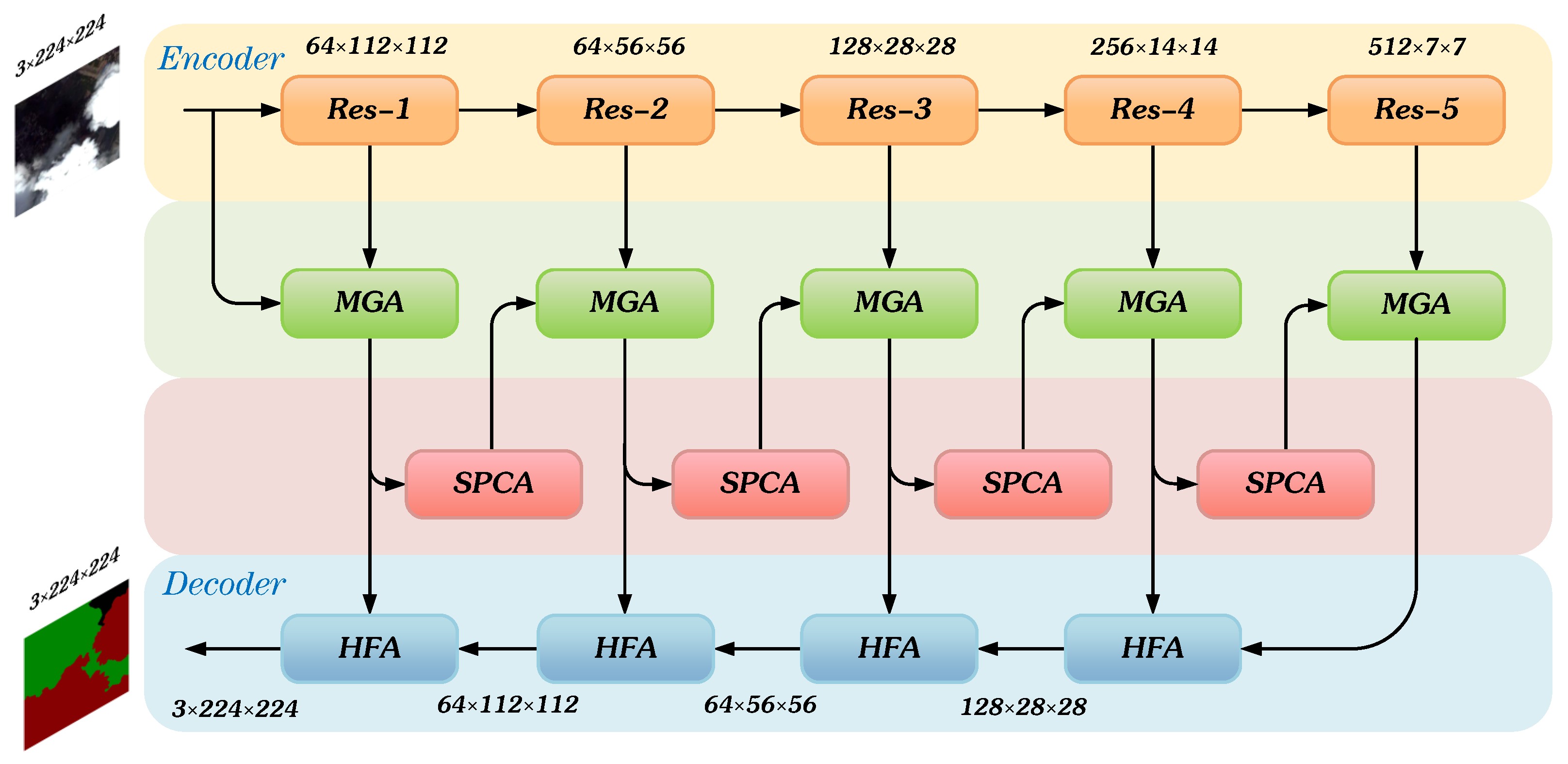
Figure 1. The structure of CRSNet. Res-i are the different levels of ResNet-18. MGA is Multi-scale Global Attention Module. SPCA is Strip Pyramid Channel Attention Module. HFA is Hierarchical Feature Aggregation Module. The size of input and output is 3 × 224 × 224. In the process of encoding and decoding, pictures are extracted into features of various sizes.
Remotesensing 15 01664 g001
Figure 2. The structure of the SEWeight module. GAP represents global average pooling, each channel is downsampled to 1 × 1 × channel size, and the weight of the channel is adaptively obtained through two full connection layers.
Remotesensing 15 01664 g002
Figure 3. The structure of SPCA. C, H and W represent the number of channels, height and width of the feature.
Remotesensing 15 01664 g003
Figure 4. The structure of MGA. HMC represents the Hierarchical Multi-scale Convolution module. MLP represents Multi-layer perceptron neural networks.
Remotesensing 15 01664 g004
Figure 5. The structure of HMC.
Remotesensing 15 01664 g005
Figure 6. The structure of HFA. C, H and W represent the number of channels, height and width of the featrue.
Remotesensing 15 01664 g006
Figure 7. The first line is some training data of the Cloud and Cloud Shadow Dataset, and the second line is some training data of the CSWV.
Remotesensing 15 01664 g007
Figure 8. Heatmap in the ablation experiment. Red indicates that the classification weight of the target category is high, and blue is the opposite.
Remotesensing 15 01664 g008
Figure 9. Prediction results of different models on Cloud and Cloud Shadow Dataset. Black, red and green represent the ground, cloud and cloud shadow, respectively. The yellow square frame marks the parts with significant differences.
Remotesensing 15 01664 g009
Figure 10. Prediction results of different models on CSWV. Black, purple and white represent the ground, cloud and snow, respectively. (a) Test image; (b) ACFNet; (c) OCRNet; (d) SegNet; (e) DFN; (f) DeepLabV3Plus; (g) CSAMNet; (h) CRSNet; (i) Label.
Remotesensing 15 01664 g010
Table 1. MIoU of different group sizes.
Kernel SizeGroup SizeMIoU
3,5,7,94,8,16,1694.13%
3,5,7,91,2,4,894.32%
3,5,7,916,16,16,1694.33%
3,5,7,92,4,8,1694.43%
Table 2. Ablation Experiment.
MethodMoiU on Cloud and Cloud Shadow (%)MoiU on CSWV (%)
ResNet-1892.9883.18
ResNet18 + SPCA93.6284.63
ResNet18 + SPCA + HFA 93.8685.43
ResNet18 + SPCA + HFA93.9286.25
ResNet18 + SPCA + HFA + MGA 94.1887.04
ResNet18 + SPCA + HFA + MGA94.4387.52
Table 3. Comparison of evaluation metrics of different models on Cloud and Cloud Shadow Dataset. In addition to the overall PA, MPA and MIoU, we calculated pixel accuracy for cloud, shadow and ground, respectively. Symbol “_” indicates no pre-training.
Class Pixel AccuracyOverall Results
MethodLand (%)Cloud (%)Shadow (%)PA (%)MPA (%)MIoU (%)
SegNet95.3594.5391.3194.5493.7387.52
UNet96.4496.0593.5795.9095.3590.39
DeepLabV3plus96.7896.3192.4795.9895.1890.65
HRNet97.1295.9992.9796.2195.3691.15
OCRNet97.3395.8992.7196.2795.3191.20
ENet97.3796.1893.1396.4295.5691.60
ShuffleNetV297.1096.7894.1296.5696.0091.89
Dual_branch_Network97.7196.6894.0096.8896.1392.66
CSAMNet97.7296.8594.9997.1096.5293.12
PADANet98.1096.5994.1197.1096.2693.14
PSPNet97.8697.0794.6197.6596.5193.29
DABNet98.0097.2394.6797.3096.6393.58
CRSNet 97.9396.8795.4497.3096.7593.59
CRSNet98.2597.5995.4597.6697.1094.43
Table 4. Comparison of evaluation metrics of different models on CSWV Dataset. Symbol “_” indicates no pre-training.
MethodPA (%)MPA (%)MIoU (%)
ENet91.2589.4082.17
PADANet91.3389.6282.20
ESPNetV2 [54]91.6689.9382.74
CCNet [55]91.7990.1483.10
HRNet91.9090.7083.19
PVT [56]91.8590.4483.35
DDRNet [57]91.7590.1383.36
PSPNet91.9590.4583.53
BiseNetV291.9890.2783.81
ACFNet [58]92.3090.7584.44
OCRNet92.6091.1484.81
SegNet92.8191.6185.12
DFN [59]93.2292.1086.22
DeeplabV3plus93.5292.1786.72
CRSNet 93.6692.3886.95
CRSNet94.0193.4687.52
Disclaimer/Publisher’s Note: The statements, opinions and data contained in all publications are solely those of the individual author(s) and contributor(s) and not of MDPI and/or the editor(s). MDPI and/or the editor(s) disclaim responsibility for any injury to people or property resulting from any ideas, methods, instructions or products referred to in the content.