Article

Multi-Scale and Multi-Stream Fusion Network for Pansharpening

1
School of Electrical and Information Engineering, Zhengzhou University, Zhengzhou 450001, China
2
School of Computer Science, Wuhan University, Wuhan 430072, China
3
School of Microelectronics and Communication Engineering, Chongqing University, Chongqing 400044, China
4
National Research Council, Institute of Methodologies for Environmental Analysis (CNR-IMAA), 85050 Tito Scalo, Italy
5
NBFC (National Biodiversity Future Center), 90133 Palermo, Italy
6
School of Engineering, University of British Columbia, Kelowna, BC V1V 1V7, Canada
*
Author to whom correspondence should be addressed.
Remote Sens. 2023, 15(6), 1666; https://doi.org/10.3390/rs15061666
Submission received: 28 January 2023 / Revised: 14 March 2023 / Accepted: 16 March 2023 / Published: 20 March 2023
(This article belongs to the Section Remote Sensing Image Processing)

Abstract

:
Pansharpening refers to the use of a panchromatic image to improve the spatial resolution of a multi-spectral image while preserving spectral signatures. However, existing pansharpening methods are still unsatisfactory at balancing the trade-off between spatial enhancement and spectral fidelity. In this paper, a multi-scale and multi-stream fusion network (named MMFN) that leverages the multi-scale information of the source images is proposed. The proposed architecture is simple, yet effective, and can fully extract various spatial/spectral features at different levels. A multi-stage reconstruction loss was adopted to recover the pansharpened images in each multi-stream fusion block, which facilitates and stabilizes the training process. The qualitative and quantitative assessment on three real remote sensing datasets (i.e., QuickBird, Pléiades, and WorldView-2) demonstrates that the proposed approach outperforms state-of-the-art methods.

1. Introduction

Remote sensing imaging is an important means by which to obtain Earth object information as high-resolution remote sensing images that are crucial in the interpretation of complex Earth objects. Due to physical limitations, a single type of satellite sensor cannot acquire a multi-spectral (MS) image with both high spatial and spectral resolution. An MS image is generally characterized by high spectral resolution but low spatial resolution, while a panchromatic (PAN) image has the opposite characteristic. However, in many practical applications, such as complex Earth feature interpretation [1,2], change detection [3,4], and land cover classification [5], high spatial and spectral resolutions are both crucial for a good analysis. Compared with hardware improvements, pansharpening provides a better solution to alleviate this problem and has gained much more attention in the remote sensing community. Pansharpening is referred to the generation of a desired high-resolution multi-spectral (HR MS) image from an MS image and a simultaneously acquired PAN image. Over the past decades, various pansharpening methods have been developed [6,7,8]. Classic and deep learning (DL)-based methods are two significant categories among the existing pansharpening methods.
Classic methods mostly use hand-crafted priors derived from basic assumptions or variational optimization procedures to fuse the low-resolution MS (LR MS) image and the PAN image. For instance, the component substitution (CS)-based methods assume that high-resolution PAN images can entirely or partially replace the principal component after the linear transformation of LR MS images. However, due to the differences in the spectral responses between the MS and PAN sensors, CS-based methods often suffer from severe spectral distortions. Another historical category is based on the use of multi-resolution analysis (MRA) frameworks to extract PAN details. The hypothesis behind the approaches in this class is that the missing high spatial details of the LR MS image can be obtained by extracting them from the PAN image via multi-scale decomposition. However, MRA-based pansharpening results are affected by both detailed extraction and injection procedures. For instance, unreasonable extraction approaches and ineffective injection coefficients may produce insufficient details, which can cause blur effects or artifacts in the final results. To achieve a better tradeoff between spectral information and spatial details, variational model (VM)-based methods use data and regularization terms to guide the pansharpening process. However, several approaches rely upon complex variational models requiring time-consuming optimization procedures to be solved.
Recently, the advanced capabilities of getting non-linear representations using convolutional neural networks (CNNs) and deep learning have achieved breakthroughs in solving the pansharpening task. However, the existing deep learning (DL)-based pansharpening methods often encounter three challenges, which are stated as follows:
  • Some DL-based methods combine all the input data together, but, in this way, they lose the possibility to independently analyze the inputs of the fusion process that are represented by the MS and PAN images;
  • Most fusion models process the source images separately and neglect their spectral/spatial correlations;
  • The use of the fixed-scale information of the input images limits the pansharpening performance.
Therefore, there is still room for improvement in pansharpening to enhance the spatial resolution while preserving the spectral information.
To address the above issues, in this paper, we propose a multi-scale and multi-stream fusion network (MMFN) for pansharpening. More specifically, we developed a multi-stream fusion block that gets the best from the input images’ spectral/spatial correlation and from the data, taking them as a separate source of information. The MS, PAN, and the concatenation of the two above-mentioned images were separately inputted to shallow convolution layers and deep convolution networks. Moreover, we downsampled the source images twice to extract multi-scale features, which can avoid the loss of spectral and spatial information. Additionally, we designed a multi-stage image reconstruction to recover the desired HR MS image. That is, for each multi-stream fusion block, a loss function was built, which can boost the training process and promote high-resolution MS images close to ground-truth images.
The main contributions of this paper can be summarized as follows:
  • Multi-scale and multi-stream strategies. We combined the multi-scale and multi-stream strategies to build a hybrid network structure for pansharpening extracting both shallow and deep features at different scales;
  • Multi-stream fusion network. On the basis of multi-scale and multi-stream strategies, we introduced a multi-stream fusion network, which separately leverages spectral and spatial information in the MS and PAN images. Simultaneously, we considered the pansharpening problem as a super-resolution task that concatenates the PAN and MS images to further extract spatial details;
  • Multi-scale information injection. We make full use of the multi-scale information of the input (MS and PAN) images by exploiting downsampling and upsampling operations. At each scale, the information of the original MS image is injected through a multi-scale loss.
The remainder of this paper is organized as follows. Section 2 briefly reviews the existing pansharpening methods. Section 3 presents the proposed pansharpening approach. Section 4 shows the experimental results. Finally, in Section 5, the conclusions are drawn.

2. Related Works

2.1. Traditional Pansharpening

The first model-based methods devoted to solving the pansharpening problem belong to the component substitution (CS) and the multi-resolution analysis (MRA) classes [6]. Early stage CS-based techniques include the intensity–hue-saturation (IHS) [9], the principle component analysis (PCA) [10], and the Gram–Schmidt (GS) transform [11]. These methods assume that the HR PAN image can substitute the principal component of the LR MS image projected into a new domain using one of the above-mentioned transformations. Aiazzi et al. [12] proposed an adaptive CS-based pansharpening method using multivariate regression analysis of the two inputs. Garzelli et al. [13] designed a band-dependent-spatial-detail (BDSD) model that extracts the optimal detail image from the PAN image for each MS band. A robust estimator based on this model has recently been proposed in [14]. Choi et al. [15] exploited the idea of the partial replacement proposing the so-called PRACS approach. Instead, Kang et al. presented in [16] an image matting model-based (MMP) component substitution pansharpening method. To alleviate the well-known spectral distortion problem for CS outcomes, researchers developed MRA-based solutions. Representative MRA-based methods include the generalized Laplacian pyramid (GLP) [17], the contourlet transformation [18], the curvelet transformation [19], and the use of non-linear morphological filters [20]. Recently, a new view of seeing the MRA framework has been developed and the detail extraction is efficiently addressed by the simple difference between the PAN image and its low-pass version [21,22] leading to new solutions achieving a high performance with a limited computational burden [23,24,25,26,27]. In this case, to overcome the issue about the limited knowledge of the shape of the spatial filters to generate the low-pass versions of the PAN image, deconvolution approaches have recently been designed [28,29].
Some promising model-based methods are the VM ones [30], which use regularization terms based on images’ prior information to solve the pansharpening (ill-posed) problem. Palsson et al. [31] presented a total variation (TV)-based pansharpening method, which encourages noise removal and preserves the edge detail information of an image. To further reduce spectral distortion, Duran et al. [32] utilized the image self-similarity, which has been applied to the PAN image to establish the nonlocal relationships among the patches of the final result. Chen et al. [33] combined local spectral consistency and dynamic gradient sparsity to simultaneously implement image registration and fusion (SIRF). Liu et al. [34] exploited structural sparsity between the LR MS image and the desired HR MS image and spectral–spatial low-rank priors. In [35], Khademi et al. incorporated an adaptive Markov random field (MRF) prior into the Bayesian framework to restore pansharpened results. Finally, hyper-Laplacian prior-based [36], local gradient constraints-based [37], texture space-based [38], and gradient sparse representation-based [39] approaches have also achieved interesting performances.

2.2. Deep Learning-Based Pansharpening

Deep learning-based methods have recently shown great potential for pansharpening thanks to their powerful nonlinear mapping capability. A comprehensive review about the topic with a critical comparison of widely-used approaches together with a freely distributed toolbox can be found in [40]. The deep learning-based pansharpening methods can be divided roughly into two categories: supervised and unsupervised.
Supervised pansharpening methods require the generation of low-resolution MS images by exploiting the original MS images as ground-truth. Masi et al. [41] attempted first to apply a network for single-image super-resolution [42] to fuse PAN and MS images. This pansharpening method, the so-called PNN, uses a three-layer convolutional neural network (CNN) to construct the map between the inputs and the desired HRMS image. Similarly, Yang et al. [43] proposed a deep network architecture (PanNet) to improve the pansharpening accuracy in terms of spatial and spectral preservation. Scarpa et al. [44] proposed a fast and high-quality target-adaptive CNN (TACNN)-based pansharpening method. To fully make use of the respective information of MS and PAN images, Liu et al. [45] adopted a two-stream fusion network (ResTFNet- l 1 ) for pansharpening. Xu et al. [46] also designed a shallow and deep feature-based spatial-spectral fusion network to enhance the pansharpened results. Liu et al. [47] attempted first to explore the combination of pansharpening and generative adversarial networks (GANs), i.e., the so-called PSGAN, to produce high-quality pansharpened results. Shao et al. [48] combined the idea of an encoder with GANs for pansharpening. A first attempt to integrate classical CS and MRA frameworks with deep convolutional neural networks has been provided in [49]. A more general framework that can fuse images with an arbitrary number of bands exploiting recurrent neural networks has recently been proposed for pansharpening [50]. Wang et al. [51] used an explicit spectral-to-spatial convolution that operates on the MS data to produce an HR MS image. However, the above methods only process single-scale images and do not perform multi-scale feature extraction. Exploiting multi-scale features is of crucial importance for pansharpening, even representing a hot topic for deep neural networks. Yuan et al. [52] introduced a multi-scale feature extraction and multidepth network for pansharpening. Wei et al. [53] proposed a two-stream coupled multi-scale network to fuse MS and PAN images. Huang et al. [54] utilized a non-subsampled contourlet transform to decompose MS and PAN images into low- and high-frequency components, then trained a network with high-frequency images and obtained the fused image by combining the output of the network and the low-frequency components of the MS image. In [55], multi-scale perception dense coding has been integrated into a neural network for pansharpening. Hu et al. [56] combined multi-scale features extraction and dynamic convolutional networks to fuse MS and PAN images. Wang et al. [57] employed a multi-scale deep residual network for pansharpening. In [58], a grouped multi-scale dilated convolution was designed to sharpen MS images. Peng et al. [59] adopted multi-scale dense blocks in a global dense connection network for pansharpening. Multi-scale feature extraction and multi-scale densely connection were employed in [60] to fuse MS and PAN images. Lai et al. [61] extracted multi-scale features in an encoder-decoder network for pansharpening. Zhou et al. [62] proposed a multi-scale invertible network and heterogeneous task distilling to fully utilize the information at full resolution. A multi-scale grouping dilated block was designed in [63] to obtain fine-grain representations of multi-scale features for pansharpening. Tu et al. [64] introduced a clique-structure-based multi-scale block and a multidistillation residual information block for MS and PAN image fusion. A parallel multi-scale attention network is presented in [65] to learn residuals to be injected into the LR MS image. Huang et al. [66] combined MRA and deep learning methods, achieving the injection coefficients with multi-scale residual blocks. Jin et al. [67] decomposed the input images using Laplacian pyramids, then exploited a multi-scale network to fuse each image scale. In [68], a pyramid attention was applied to capture multi-scale features and then the latter were fused by a feature aggregation module to obtain the fused product. A multi-scale transformer with an interaction attention module was introduced in [69]. Zhang et al. [70] proposed a 3D multi-scale attention network for MS and PAN image fusion, in which 2D and 3D convolutions were compared for this task. Although these methods all use multi-scale feature extraction, they either directly perform multi-scale processing on the concatenated MS and PAN images or separately extract features from the MS and PAN images and then perform multi-scale processing. None of the state-of-the-art approaches in the literature can effectively fuse the features extracted from the combined MS and PAN images and the features separately extracted from the MS and PAN images.
The other sub-class of deep learning-based pansharpening approaches relies upon unsupervised methods. Indeed, due to the lack of ground-truth MS images, Qu et al. [71] and Uezato et al. [72] presented unsupervised ways to train models for pan-sharpening.
Finally, there are the promoting methods, belonging to the class of hybrid pansharpening solutions, that combine variational optimization-based and deep learning models, thus benefiting from both the philosophies and increasing the generalization ability of deep learning approaches, see, e.g., Refs. [73,74,75].

3. Proposed Method

The proposed method utilizes multi-scale information and a multi-stream fusion strategy to fully use different levels of features in PAN and MS images. We will introduce the problem formulation of the pansharpening task and depict the overview framework. Afterwards, the network architecture and loss function are presented in detail.

3.1. Problem Formulation

The LR MS image is denoted as M with a size of w × h × c ( M R w × h × c ), while the high-resolution PAN image is denoted as P with a size of r w × r h × 1 ( P R r w × r h × 1 ), where w, h, and c are the width, height, and number of channels of the MS image, r is the spatial scale factor between the PAN and MS images. The goal of pansharpening is to obtain an HR MS image, X, as close as to the ground-truth image, G, with a size of r w × r h × c . We designed the overall framework, which learns the pansharpened process, namely, X = f Θ n e t M , P , where f n e t and Θ represent the MMFN architecture and its parameters, respectively.

3.2. Network Architecture

Figure 1 shows the overall framework of the proposed method, including the multi-scale feature extraction, the multi-stream feature fusion, and the multi-stage image reconstruction. To fully extract the features from the input PAN and MS images, we used a multi-scale strategy to downsample the input images twice, which allows the extracted features to represent original images at different levels. We used the same multi-stream block (MSB) for each scale to fuse the downsampled PAN and MS images. Finally, the pansharpened sub-images were upsampled to recover the HR MS image using a multi-stage strategy. A detailed description is given in the following sections.

3.2.1. Multi-Scale Feature Extraction

We used a fixed scale factor to downsample the PAN and MS images. This operation can extract different levels of spectral and spatial features in both PAN and MS images and it can maximize the information usage at different scales. We denote D · as the downsampling operation. Thus, we have:
I t = D I t 1 , s , t = 2 , 3 ,
where I 1 is M ˜ or P when the downsampling of the upsampled version of the MS image or the PAN image is considered, respectively, I t (with t > 1 ) represents the downsampled version of the MS or PAN images, t and s are the scale index and the downsampling factor (equal to 2 in our case), respectively.

3.2.2. Multi-Stream Feature Fusion

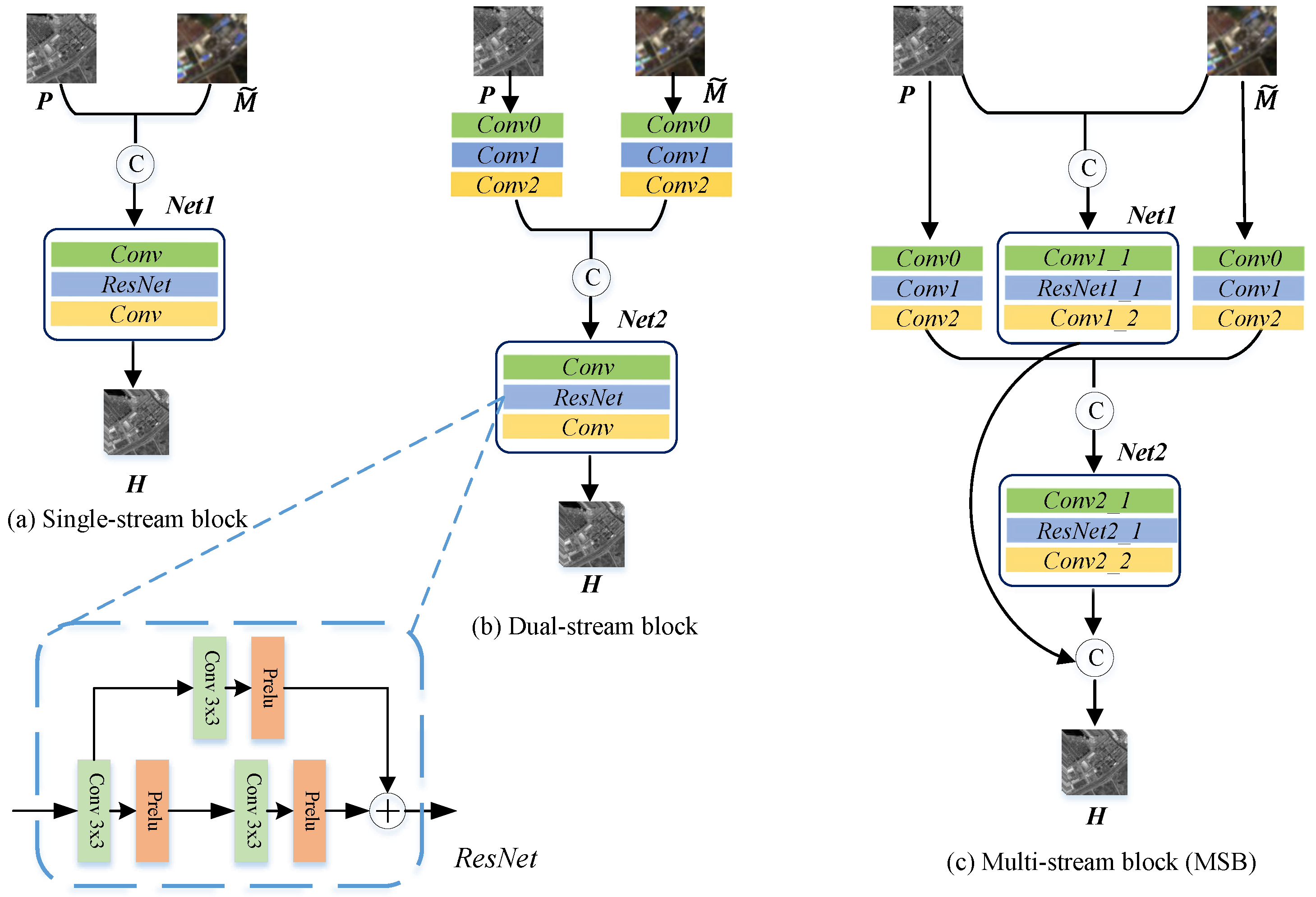
Many researchers regard the pansharpening task as a super-resolution problem that concatenates the MS and PAN images to form a single stream network for spatial information improvement, as shown in Figure 2a. However, in this way, the related spectral characteristics of the input products are ignored. Some other researchers consider that the MS and PAN images convey various independent information. The typical operation is to use the high-frequency information of the PAN image to build the missing spatial details of the MS image. However, it is hard to state that the spatial information is a typical feature related to the sole PAN image and the spectral features are only related to the MS image. This challenge motivates us to focus on developing a dual-stream fusion network (see Figure 2b), which combines all the features of the MS and PAN images.
To avoid losing information as in the case of the single-stream or the dual-stream, we leveraged a multi-stream fusion strategy to comprehensively exploit information from the spectral and spatial domains. As shown in Figure 2c, we utilized three streams, namely, PAN, MS, and fusion streams, to extract the features from the PAN data, the MS image, and the concatenation of the two inputs (i.e., MS and PAN), respectively. First, the PAN and MS streams built by three sequential convolutional layers were used to extract spatial and spectral features as follows:
F = C o n v ( C o n v ( C o n v ( P ) ) ) ,
where C o n v ( · ) denotes the convolutional layers, P is the (input) MS/PAN image, and F is the corresponding output. The fusion stream is instead fed by the concatenation of the MS, M t , and the PAN, P t , images to extract spatial-spectral features by a ResNet between two convolutional layers. Hence, we have that the spatial–spectral features, F P M S , are obtained by:
F P M S = C o n v R e s N e t C o n v [ P t , M t ] ,
where [ · ] denotes the concatenation operation and R e s N e t ( · ) is the function of ResNet as shown in Figure 2. Finally, we further fused the outputs from the three streams by the same structure as in the fusion stream, thus obtaining the output of the MSB by concatenating F P M S with the further fused features, i.e.,
H t = [ F P M S , C o n v R e s N e t C o n v [ P t , M t , F P M S ] ] ,
where H t is the output of the MSB.

3.2.3. Multi-Stage Image Reconstruction

In our work, we used the original source images and their two downsampled versions to perform a three-stage pansharpening network. All the image pairs were fed into the same multi-stream fusion block using Equation (4) for the extraction of the multi-scale fused features. As shown in Figure 1, these multi-scale features were adopted to reconstruct the multi-scale image by using reconstruction blocks, which have the same structure as the one in the fusion stream (i.e., Net 1 in Figure 2c).
F t = C o n v R e s N e t C o n v [ P t , M t , F P M S ] ,
where F t is the fused image at the t-th scale.
Afterwards, the fusion result of each RB was upsampled and concatenated with the corresponding downsampled MS image as follows:
X t = [ U F t + 1 , s , M t ˜ ] , t = 1 , 2 ,
where U · represents the upsampling operation. In our work, we have that X 3 = M 3 ˜ .
After the multi-stage fusion, the final HRMS image can be reconstructed in a residual way, thus preserving the spectral information. Hence, we have:
X = F 1 + M ˜ ,
where X is the fused (pansharpened) product.

3.3. Loss Function

During the training phase, we adopted the l 1 -norm as loss function to measure the distance between the pansharpened product and the related ground-truth (reference) image. Comparing it with the l 2 -norm, the l 1 -norm can overcome local minima reaching stable training [76]. Our work had three MSB blocks that generated pansharpening images at three different resolutions. Thus, a loss function was adopted for each block to constrain its training. Hence, the overall loss function can be written as:
L Θ = 1 3 t = 1 3 F t H R M S t 1 ,
where Θ is the set of parameters for the proposed framework, H R M S t is the downsampled version of the ground-truth image at the t-th scale, and · 1 is the l 1 -norm.

4. Experiment and Evaluations

In this section, we provide extensive experiments to validate the effectiveness of our proposed method. Moreover, three groups of ablation studies were investigated to further demonstrate the superiority of each claim.

4.1. Datasets and Metrics

Three real remote sensing datasets, captured by QuickBird, Pléiades, and WorldView-2, were used. To boost the pansharpening capability of the proposed network, we adopted data argumentation approaches, i.e., rotation, cropping, and flipping. The total number of training and testing datasets for each satellite were 4000 and 40, respectively.
Due to the lack of ground-truth datasets, we used Wald’s protocol [77] to obtain the downsampling version of both MS and PAN images (with a downsampling factor equal to 4). The degraded MS images were upsampled to the original size so that the MS image could serve as the HR MS (ground-truth) image for quality assessment.
In our study, to quantitatively evaluate the pansharpened results, six metrics with reference and a metric without reference were employed to evaluate the products at reduced resolution and at full resolution, respectively. For the metrics with reference, the correlation coefficient (CC) [12], the relative dimensionless error in synthesis (ERGAS) [78], the Q 2 n [79], the spectral angle mapper (SAM) [80], the relative average spectral error (RASE) [81], and the root mean squared error (RMSE) were used. Additionally, the metric without reference consisted of the combination of a spectral distortion ( D λ ) index and a spatial distortion ( D S ) index. It is commonly-used and known as a quality with no reference (QNR) index [82,83]. In general, the largest values of CC, Q 4 , and QNR indicate the best performance. On the other hand, the smaller the ERGAS, SAM, RASE, and RMSE are, the closer the results are to the ground-truth (reference) image.

4.2. Implementation Details

We trained the proposed framework using PyTorch [84]. The configuration of the hardware device was composed of an NVIDIA GTX 1070Ti (GPU), 48-GB RAM (Memory), and an Intel Core i5-8500 (CPU). For the training phase, an Adam optimization algorithm is used. The initial learning rate, the moment decay, and the batch size were set to 0.0001, 0.9, and 4, respectively. The input size of the LR MS image and the PAN image were set to 64 × 64 and 256 × 256 , respectively. The parameters of each convolutional layer in the MSB block and the RB block are described in Table 1. The training epochs were 400.

4.3. Results and Discussion

To fairly compare the effectiveness of the proposed MMFN, we selected thirteen state-of-the-art pansharpening methods, including seven widely used traditional ones, i.e., Inter23 [6], which is the simple upsampling to the PAN scale using a 23-tap polynomial interpolator, AWLP [6,85], BDSD [13], GSA [12], MMP [16], MTF-GLP-HPM (MGH) [21], and SIRF [33], and six deep learning-based ones, i.e., PNN [41], PanNet [43], PSGAN [47], ResTFNet- l 1 [45], TACNN [44], and MUCNN [51]. All the experiments were conducted using the set of parameters as originally indicated by the authors in the related papers. In the following, we will present the results for the two classical assessments, i.e., at reduced and full resolutions.

4.3.1. Assessment at Reduced Resolution

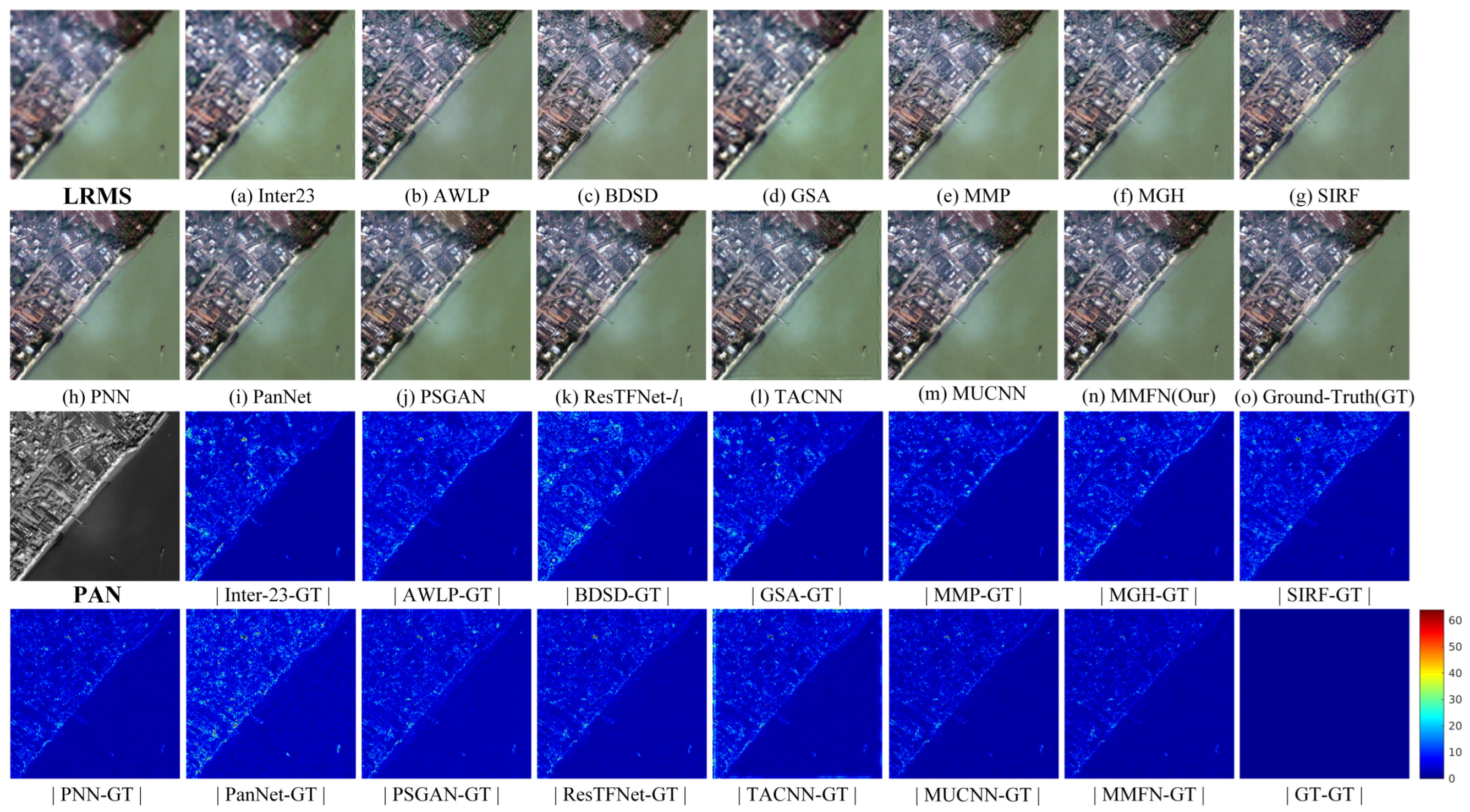
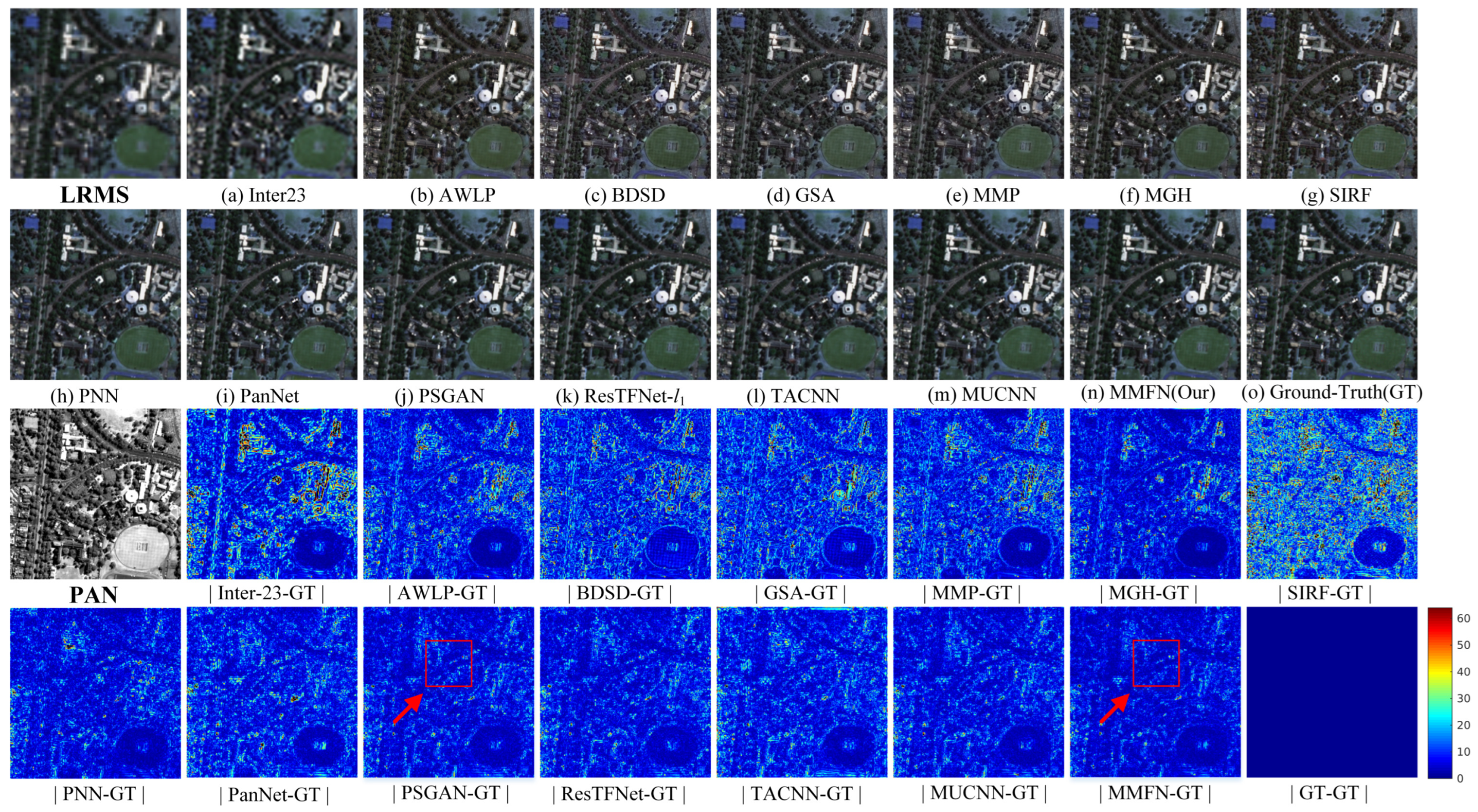
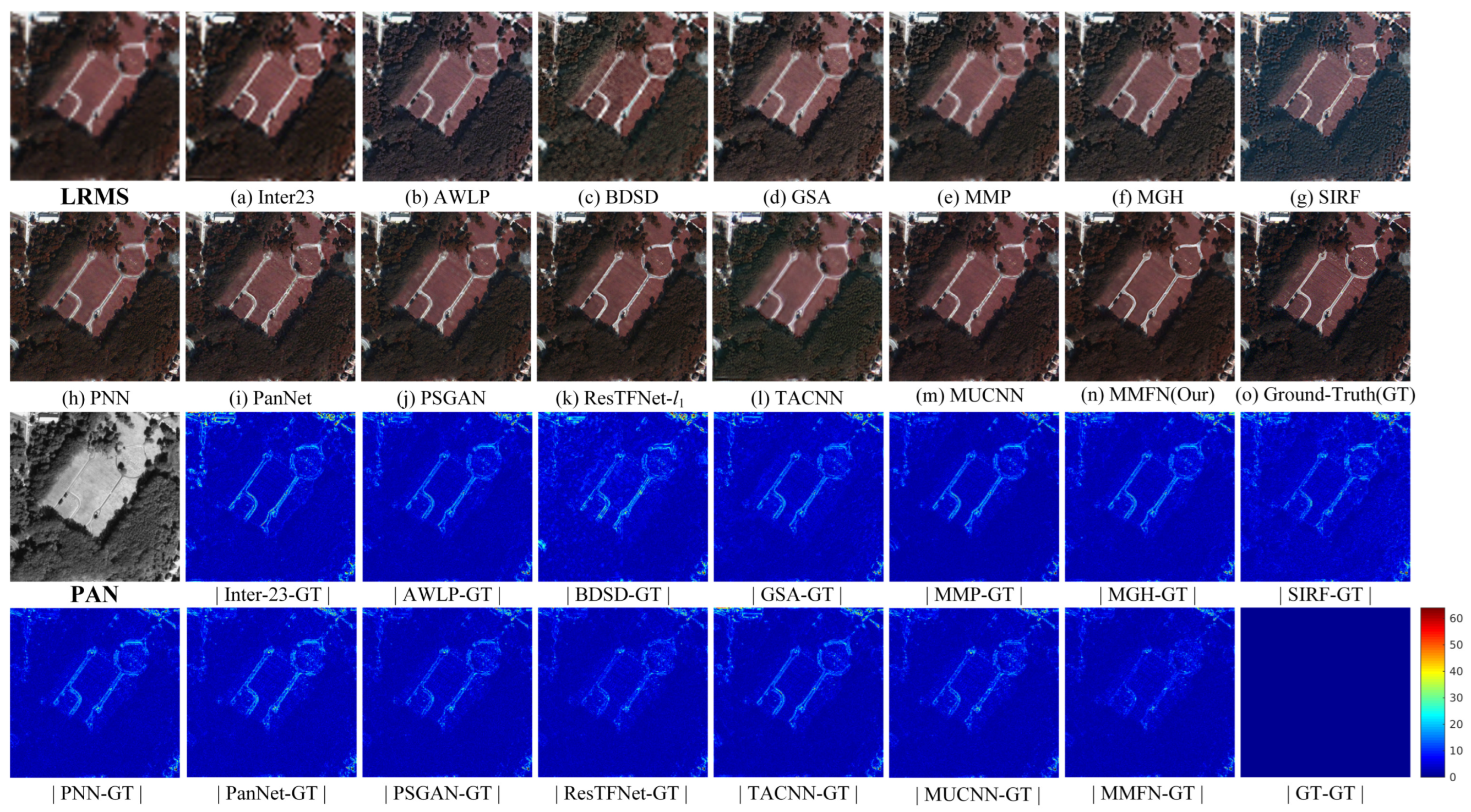
In this section, we compare the performance at reduced resolution of the proposed method with the proposed benchmark. Figure 3, Figure 4 and Figure 5 present the pansharpened results for the three datasets acquired by QuickBird, Pléiades, and WorldView-2, respectively. For the visual comparison, all the images are shown in true (RGB) color. Additionally, mean absolute errors (MAEs, by using heatmaps), namely, residual maps between pansharpened results and the related reference images, are also given. The results show that the deep learning-based methods outperform the traditional ones in terms of MAEs.
In Figure 3, compared with the ground-truth image (Figure 3o), the traditional approaches, i.e., Inter23, AWLP, BDSD, GSA, MMP, MGH, suffer from various degrees of spatial detail loss, especially some serious blurring effects generated by Inter23 and GSA methods. This is because the Inter23-based method directly utilizes a polynomial kernel (with 23 coefficients) to upsample the LRMS image without any information from the PAN image. The GSA-based method may fail to estimate the high-frequency details during the component replacement operation. Deep learning-based techniques also show poor performance in preserving spatial details, as seen from the results produced by PNN, PanNet, TACNN, and MUCNN. Although PSGAN and ResTFNet- l 1 can obtain promising pansharpened results that are close to the ground-truth image from a visual point of view, some differences still exist when observing the residual maps. By contrast, our MMFN method can achieve the best trade-off in preserving spatial details and spectral signatures, which are the closest with respect to the ground-truth ones. Table 2 reports the average quantitative performance on the QuickBird dataset including 40 groups of images by using different pansharpening methods. As shown in the table, the proposed MMFN achieves the best results for all the metrics, indicating that our approach has outstanding sharpening capabilities for reduced resolution images. The ResTFNet is also a promising method. From both a quantitative and qualitative point of view, we can state that our proposed method can achieve better pansharpening outcomes.
Similarly, in Figure 4 and Figure 5, the pansharpening results for Pléiades and WorldView-2 are depicted. Again, it is easy to observe that the performance of traditional methods is inferior with respect to deep learning-based ones. In Figure 4, the conventional methods, except for Inter23, show various degrees of spectral distortion, mainly in the wooded areas. Moreover, the color of the road is also inconsistent with the reference image. It can be found that the BDSD and GSA methods generate block effects in the vegetation areas. Deep learning-based methods instead produce better results (closer to the ground-truth image). However, spatial distortion still exists, at seen from the MAE maps. Although the performance of PSGAN and the proposed approach are similar at first glance, the residual map of the proposed approach is closer to zero, see the red boxes in the figure. In Figure 5, the SIRF method can efficiently perform spatial details enhancement. However, it suffers from severe spectral distortion, see Figure 5g. Compared with the ground-truth image, the results of AWLP, BDSD, PNN, and TACNN generate visible color distortion. Additionally, the benchmarking methods still have a loss of spatial information on the WorldView-2 dataset in terms of MAEs, see, e.g., the result of the MUCNN method. Thus, from this analysis, it is clear that the best performance is obtained by the proposed MMFN. This statement is further corroborated by the quantitative results in Table 3 and Table 4. Indeed, the proposed MMFN method achieves the best results on both the Pléiades and WorldView-2 datasets and for all the metrics. In conclusion, the generalization ability of the proposed method for reduced-resolution images is better than that of the state-of-the-art methods.

4.3.2. Full Resolution Assessment

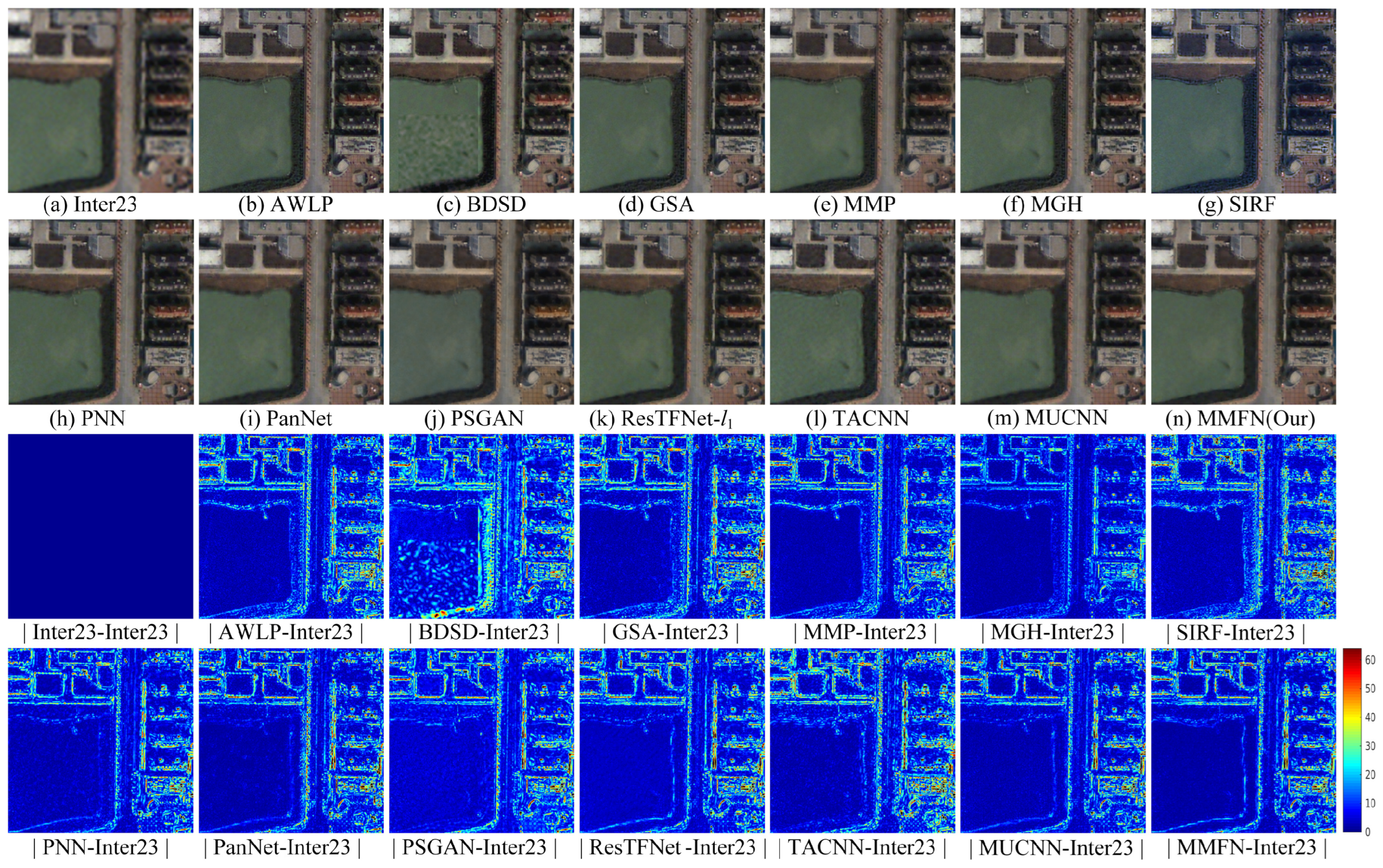
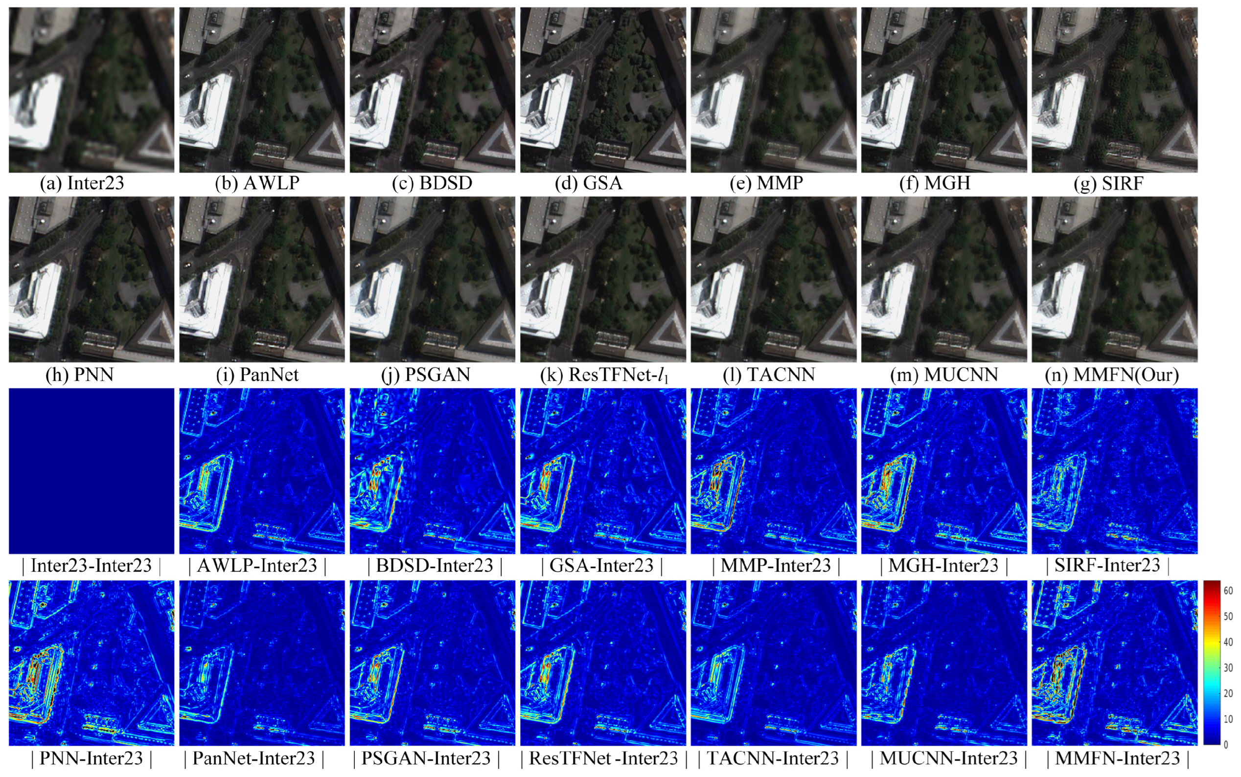
We further assess the proposed method at full resolution using datasets at the original scale without any spatial degradation to generate the ground-truth (reference) image. Figure 6, Figure 7 and Figure 8 show the qualitative comparison. The D λ , D s , and QNR metrics were used to evaluate the pansharpened performance. Inter23 obtains the best D λ value, which indicates the absence of spectral distortion. Therefore, we used the results of the Inter23-based method as the basis images from which to observe the detailed information of PAN images injected into the output images. For visual comparison, we still adopted a residual representation calculating the difference between the pansharpened result and Inter23 to display the injected details. It is observed that the DL-based methods inject more structures and textures than the compared traditional methods, see, e.g., the residual images for the QuickBird dataset in Figure 6. BDSD transfers the wrong details into the pansharpened product, leading to noise effects on green areas, see Figure 6c. From a visual point of view, lawn areas should be smooth without containing any detail. Significant spectral distortion still exists in the result of the SIRF-based method, see Figure 6g. Among the traditional methods, the AWLP, GSA, MMP, and MGH-based approaches can hardly transfer precise edges into the pansharpened results, as shown in the related MAEs in Figure 6. It is clear from Figure 6j that PSGAN produces spectral distortion in the buildings with an orange-like color (the right side of the image). A similar phenomenon is that partial edges around green areas can be retained in the MAE results of PNN, PanNet, and TACNN-based methods. Although the ResTFNet, MUCNN, and the proposed method have highly similar results, the blurring effects and the noise cannot be removed in green vegetation areas. Objective evaluations are reported in the last three columns of Table 2. We find that the proposed method obtains a high performance in terms of D S , and almost the best QNR metrics. Overall, the full-resolution experiments on the QuickBird dataset are satisfying.
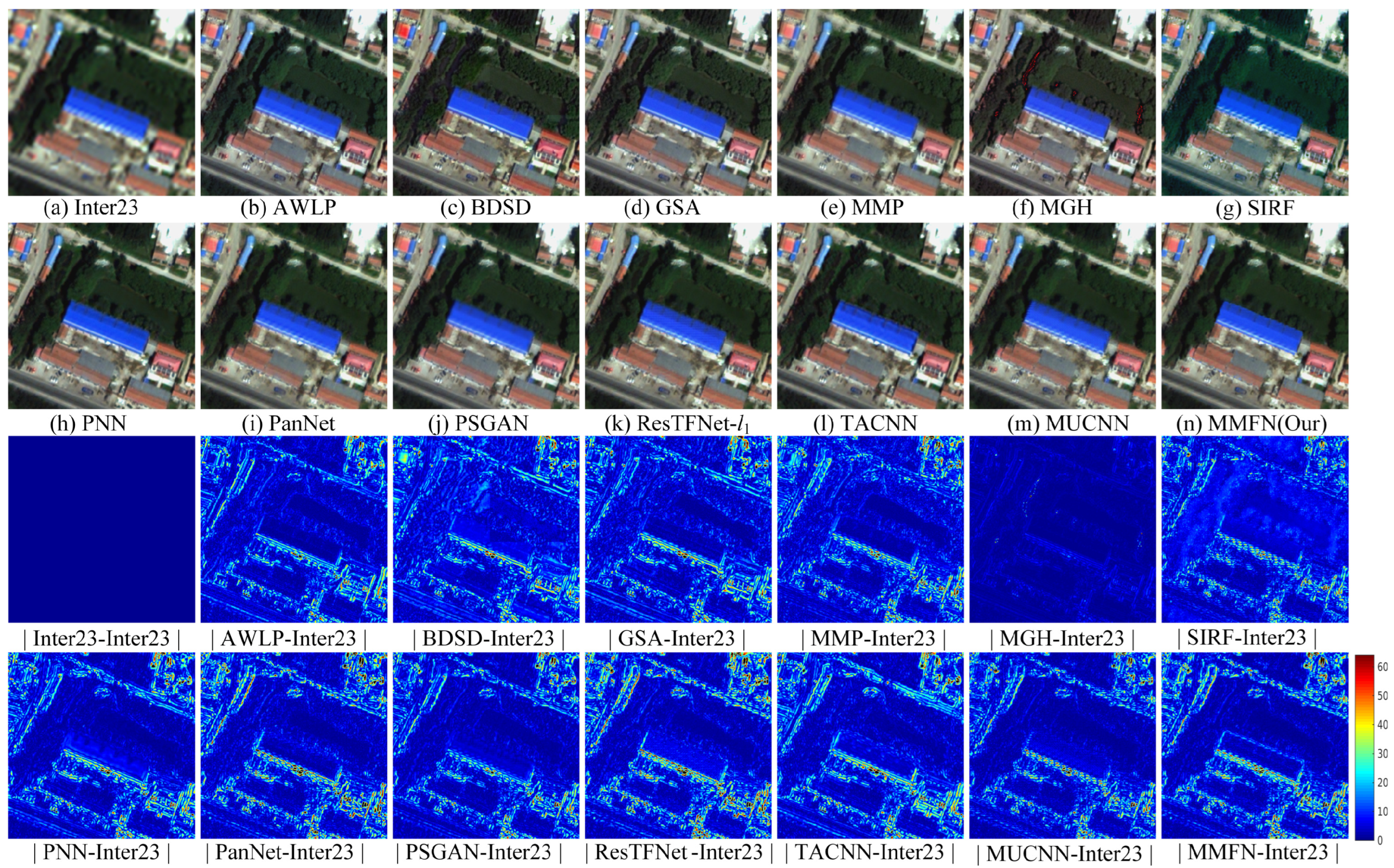
A similar visual analysis can be performed in Figure 7 and Figure 8 for the other two datasets (i.e., Pléiades and WorldView-2). It is easy to see that the proposed MMFN achieves the best trade-off between spatial and spectral consistency. Furthermore, objective results mark the high performance of the proposed approach; see the last three columns of Table 3 and Table 4, again. Indeed, the proposed MMFN has a promising fusion performance, balancing the trade-off between spatial enhancement and spectral fidelity, thanks to the use of the multi-scale information and the multi-stream fusion strategy.

4.3.3. Parameter Numbers vs. Model Performance

We added a comparative experiment evaluating the running times of deep learning methods. We conducted experiments on a hardware device with an Intel(R) Xeon(R) Gold 5117 CPU @ 2.00 GHz and 128 GB memory. We used Python 3.9 and PyTorch 1.11 as the programming language and deep learning framework, respectively. We tested running times for both full and reduced resolution MS images with a batch size of 4. We measured the average execution times for processing a single input on the CPU. We used the Python built-in timer to measure the execution times, repeating each measurement 10 times to ensure statistical significance. The results are shown in Table 5. Although our method is not the most time-efficient one (because it processes more features generated at different scales), it exploits fewer parameters than PSGAN and ResTFNet- l 1 , thus having a shorter running time. Furthermore, while our method is not as time-efficient as PNN, PanNet, MUCNN, and TACNN, it achieves a better pansharpening performance.

4.4. Ablation Studies

In this section, we provide three groups of ablation studies to demonstrate each claim of the proposed framework.

4.4.1. Ablation Study about Different Scales

To investigate the influence of the number of scales on the pansharpening performance, we compared the results of six different scales by using a fixed multi-stream fusion network. From Figure 9, it can be observed that increasing the number of scales cannot continuously improve the pansharpening performance in terms of objective evaluation. Most evaluation metric values indicate that the performance of the multi-scale (scale number = 3) results is better than that of the other scales. Additionally, as the number of scales increases, the processing time increases. Therefore, the scale number equal to three represents a good choice for our approach.
As shown in Figure 10, by observing the residual maps between the results of the different scales and the reference image, the spectral distortion and spatial distortion can be significantly reduced, increasing the number of scales. It is also straightforward to see that three scales represent the best result among the three presented in the figure.

4.4.2. Ablation Study about Different Streams

To verify the effectiveness of the choice of a number of streams equal to three, the single-stream (stream number = 1) fusion and the dual-stream (stream number = 2) fusion were investigated, fixing the multi-scale network.
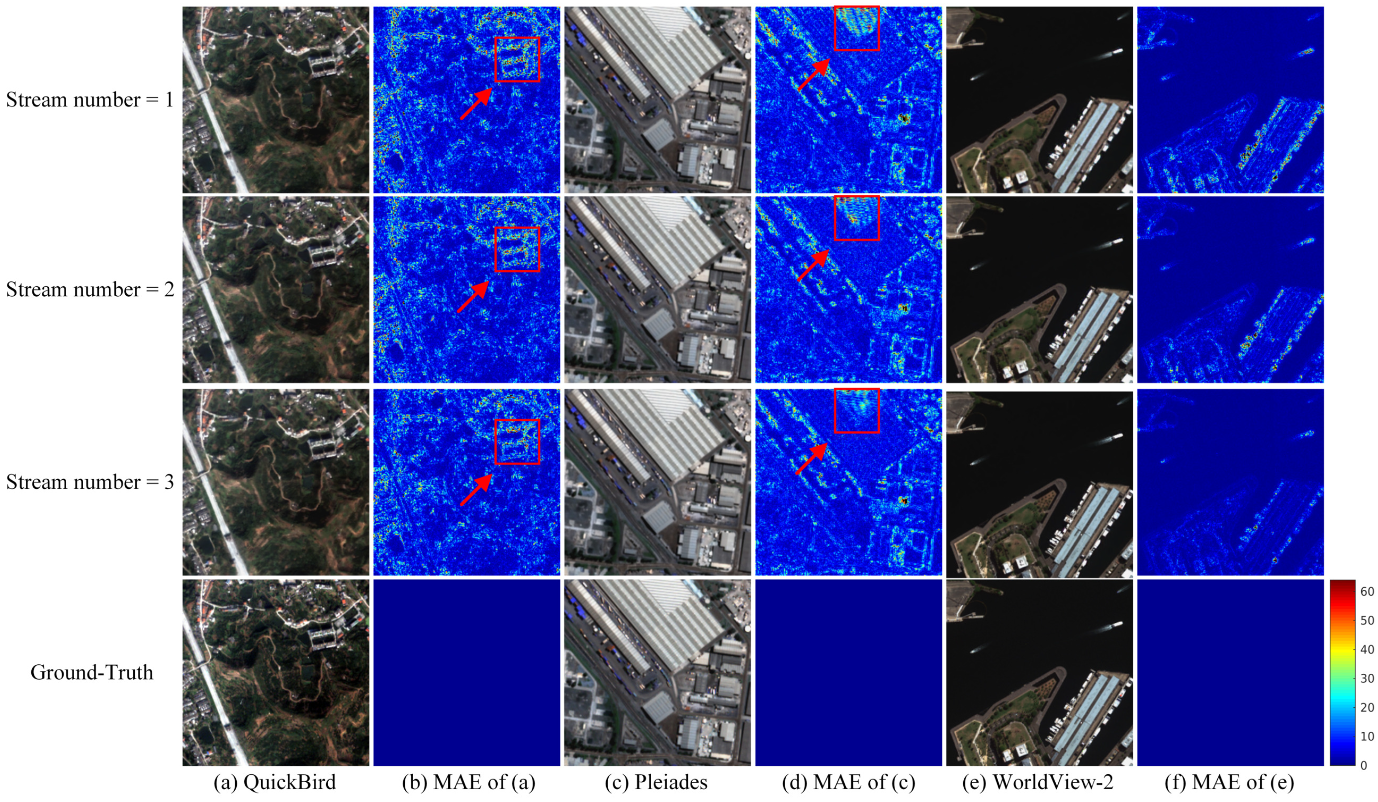
The quantitative comparison is presented in Figure 11. The results of the multi-stream block using three streams are better than those of single-stream and dual-stream fusion blocks. This is because the sole use of an architecture with single-stream or dual-stream fusion cannot guarantee the full merge of the spatial details of the PAN image together with the spectral information of the MS image. In addition, Figure 12 shows the qualitative results on the three real remote sensing datasets, varying the number of streams. As the number of streams increases, the spectral and spatial distortions decrease. Thus, the above-mentioned ablation studies confirm the validity of the choices made (the number of scales and streams both equal to three).

4.4.3. Ablation Study about Different numbers of Residual Blocks

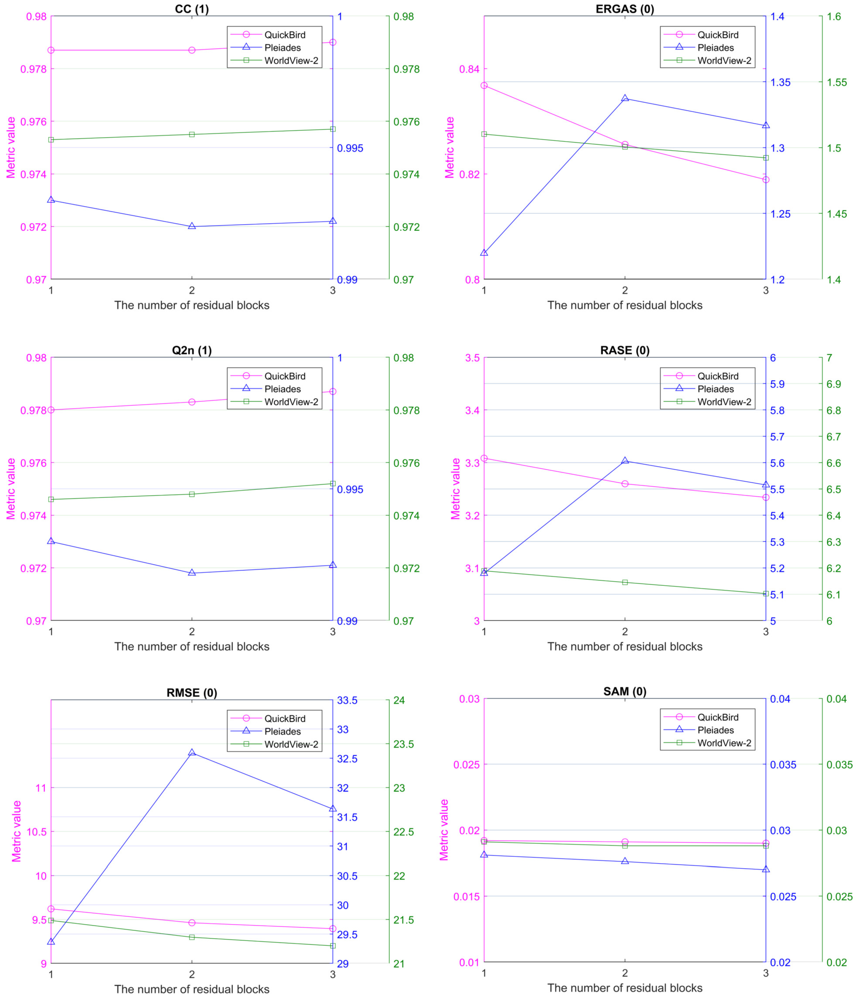
To assess the effect of the number of residual blocks in the MSB module on the results, we experimentally tested the impact of using one, two, and three residual blocks. The experimental results shown in Figure 13 indicate that increasing the number of residual blocks leads to a slight improvement in performance on WorldView-2 and QuickBird datasets. However, on the Pléiades dataset, there was a decrease in performance as the number of residual blocks increases. This is because the simplest model structure is enough for the Pléiades dataset. Considering that increasing the number of residual blocks also increases the complexity and computational cost of the network, leading to overfitting and longer training times, the simplest structure was chosen.

5. Conclusions

This paper proposed a multi-scale and multi-stream fusion network (MMFN), which is simple but effective for pansharpening. Different levels of spectral/spatial information contained in the MS and PAN images was obtained first by using a multi-scale strategy. Afterwards, a multi-stream fusion block was adopted to fully fuse the MS and PAN images, preserving their spatial and spectral characteristics. Additionally, to constrain the training process, we developed a multi-stage reconstruction approach, setting the same loss function for each fusion block. The proposed method was assessed on three real remote sensing datasets acquired by three different sensors. The reduced and full resolution assessments demonstrated the validity of the proposed approach.

Author Contributions

Conceptualization, L.J. and S.W.; methodology, L.J.; software, S.W.; validation, R.R., L.C. and D.Z.; formal analysis, S.W.; investigation, G.V.; resources, D.Z.; data curation, S.W.; writing—original draft preparation, L.J.; writing—review and editing, L.J., R.R. and G.V.; visualization, L.J. and R.R.; supervision, S.W. and G.V.; project administration, L.J.; funding acquisition, L.J. All authors have read and agreed to the published version of the manuscript.

Funding

This research was funded by National Natural Science Foundation of China (NSFC) under Grant 62101502, in part by China Postdoctoral Science Foundation under Grant 2022T150596, and in part by Postdoctoral Research Grant in Henan Province under Grant 202101012.

Data Availability Statement

Not applicable.

Conflicts of Interest

The authors declare no conflict of interest.

References

  1. Souza, C., Jr.; Firestone, L.; Silva, L.M.; Roberts, D. Mapping forest degradation in the Eastern Amazon from SPOT 4 through spectral mixture models. Remote Sens. Environ. 2003, 87, 494–506. [Google Scholar] [CrossRef]
  2. Yang, B.; Kim, M.; Madden, M. Assessing optimal image fusion methods for very high spatial resolution satellite images to support coastal monitoring. GISci. Remote Sens. 2012, 49, 687–710. [Google Scholar] [CrossRef]
  3. Shalaby, A.; Tateishi, R. Remote sensing and GIS for mapping and monitoring land cover and land-use changes in the Northwestern coastal zone of Egypt. Appl. Geogr. 2007, 27, 28–41. [Google Scholar] [CrossRef]
  4. Wu, C.; Du, B.; Cui, X.; Zhang, L. A post-classification change detection method based on iterative slow feature analysis and Bayesian soft fusion. Remote Sens. Environ. 2017, 199, 241–255. [Google Scholar] [CrossRef]
  5. Kumar, U.; Milesi, C.; Nemani, R.R.; Basu, S. Multi-sensor multi-resolution image fusion for improved vegetation and urban area classification. Int. Arch. Photogramm. Remote Sens. Spat. Inf. Sci. 2015, 40, 51–58. [Google Scholar] [CrossRef] [Green Version]
  6. Vivone, G.; Alparone, L.; Chanussot, J.; Dalla Mura, M.; Garzelli, A.; Licciardi, G.A.; Restaino, R.; Wald, L. A critical comparison among pansharpening algorithms. IEEE Trans. Geosci. Remote Sens. 2014, 53, 2565–2586. [Google Scholar] [CrossRef]
  7. Meng, X.; Shen, H.; Li, H.; Zhang, L.; Fu, R. Review of the pansharpening methods for remote sensing images based on the idea of meta-analysis: Practical discussion and challenges. Inf. Fusion 2019, 46, 102–113. [Google Scholar] [CrossRef]
  8. Yilmaz, C.S.; Yilmaz, V.; Gungor, O. A theoretical and practical survey of image fusion methods for multispectral pansharpening. Inf. Fusion 2022, 79, 1–43. [Google Scholar] [CrossRef]
  9. Rahmani, S.; Strait, M.; Merkurjev, D.; Moeller, M.; Wittman, T. An adaptive IHS pan-sharpening method. IEEE Geosci. Remote Sens. Lett. 2010, 7, 746–750. [Google Scholar] [CrossRef] [Green Version]
  10. Kwarteng, P.; Chavez, A. Extracting spectral contrast in Landsat Thematic Mapper image data using selective principal component analysis. Photogramm. Eng. Remote Sens. 1989, 55, 339–348. [Google Scholar]
  11. Laben, C.A.; Brower, B.V. Process for Enhancing the Spatial Resolution of Multispectral Imagery Using Pan-Sharpening. U.S. Patent 6,011,875, 4 January 2000. pp. 1–9. [Google Scholar]
  12. Aiazzi, B.; Baronti, S.; Selva, M. Improving component substitution pansharpening through multivariate regression of MS + Pan data. IEEE Trans. Geosci. Remote Sens. 2007, 45, 3230–3239. [Google Scholar] [CrossRef]
  13. Garzelli, A.; Nencini, F.; Capobianco, L. Optimal MMSE pan sharpening of very high resolution multispectral images. IEEE Trans. Geosci. Remote Sens. 2007, 46, 228–236. [Google Scholar] [CrossRef]
  14. Vivone, G. Robust band-dependent spatial-detail approaches for panchromatic sharpening. IEEE Trans. Geosci. Remote Sens. 2019, 57, 6421–6433. [Google Scholar] [CrossRef]
  15. Choi, J.; Yu, K.; Kim, Y. A new adaptive component-substitution-based satellite image fusion by using partial replacement. IEEE Trans. Geosci. Remote Sens. 2010, 49, 295–309. [Google Scholar] [CrossRef]
  16. Kang, X.; Li, S.; Benediktsson, J.A. Pansharpening with matting model. IEEE Trans. Geosci. Remote Sens. 2013, 52, 5088–5099. [Google Scholar] [CrossRef]
  17. Aiazzi, B.; Alparone, L.; Baronti, S.; Garzelli, A.; Selva, M. MTF-tailored multiscale fusion of high-resolution MS and Pan imagery. Photogramm. Eng. Remote Sens. 2006, 72, 591–596. [Google Scholar] [CrossRef]
  18. Shah, V.P.; Younan, N.H.; King, R.L. An efficient pan-sharpening method via a combined adaptive PCA approach and contourlets. IEEE Trans. Geosci. Remote Sens. 2008, 46, 1323–1335. [Google Scholar] [CrossRef]
  19. Choi, M.; Kim, R.Y.; Nam, M.R.; Kim, H.O. Fusion of multispectral and panchromatic satellite images using the curvelet transform. IEEE Geosci. Remote Sens. Lett. 2005, 2, 136–140. [Google Scholar] [CrossRef]
  20. Restaino, R.; Vivone, G.; Dalla Mura, M.; Chanussot, J. Fusion of multispectral and panchromatic images based on morphological operators. IEEE Trans. Image Process. 2016, 25, 2882–2895. [Google Scholar] [CrossRef] [Green Version]
  21. Vivone, G.; Restaino, R.; Dalla Mura, M.; Licciardi, G.; Chanussot, J. Contrast and error-based fusion schemes for multispectral image pansharpening. IEEE Geosci. Remote Sens. Lett. 2013, 11, 930–934. [Google Scholar] [CrossRef] [Green Version]
  22. Alparone, L.; Baronti, S.; Aiazzi, B.; Garzelli, A. Spatial methods for multispectral pansharpening: Multiresolution analysis demystified. IEEE Trans. Geosci. Remote Sens. 2016, 54, 2563–2576. [Google Scholar] [CrossRef]
  23. Vivone, G.; Dalla Mura, M.; Garzelli, A.; Restaino, R.; Scarpa, G.; Ulfarsson, M.O.; Alparone, L.; Chanussot, J. A New Benchmark Based on Recent Advances in Multispectral Pansharpening: Revisiting pansharpening with classical and emerging pansharpening methods. IEEE Geosci. Remote Sens. Mag. 2020, 9, 53–81. [Google Scholar] [CrossRef]
  24. Restaino, R.; Vivone, G.; Addesso, P.; Chanussot, J. A pansharpening approach based on multiple linear regression estimation of injection coefficients. IEEE Geosci. Remote Sens. Lett. 2019, 17, 102–106. [Google Scholar] [CrossRef]
  25. Vivone, G.; Restaino, R.; Chanussot, J. A regression-based high-pass modulation pansharpening approach. IEEE Trans. Geosci. Remote Sens. 2017, 56, 984–996. [Google Scholar] [CrossRef]
  26. Vivone, G.; Marano, S.; Chanussot, J. Pansharpening: Context-based generalized Laplacian pyramids by robust regression. IEEE Trans. Geosci. Remote Sens. 2020, 58, 6152–6167. [Google Scholar] [CrossRef]
  27. Vivone, G.; Restaino, R.; Chanussot, J. Full scale regression-based injection coefficients for panchromatic sharpening. IEEE Trans. Image Process. 2018, 27, 3418–3431. [Google Scholar] [CrossRef]
  28. Vivone, G.; Simões, M.; Dalla Mura, M.; Restaino, R.; Bioucas-Dias, J.M.; Licciardi, G.A.; Chanussot, J. Pansharpening based on semiblind deconvolution. IEEE Trans. Geosci. Remote Sens. 2014, 53, 1997–2010. [Google Scholar] [CrossRef]
  29. Vivone, G.; Addesso, P.; Restaino, R.; Dalla Mura, M.; Chanussot, J. Pansharpening based on deconvolution for multiband filter estimation. IEEE Trans. Geosci. Remote Sens. 2018, 57, 540–553. [Google Scholar] [CrossRef]
  30. Deng, L.J.; Vivone, G.; Guo, W.; Dalla Mura, M.; Chanussot, J. A variational pansharpening approach based on reproducible kernel Hilbert space and heaviside function. IEEE Trans. Image Process. 2018, 27, 4330–4344. [Google Scholar] [CrossRef]
  31. Palsson, F.; Sveinsson, J.R.; Ulfarsson, M.O. A new pansharpening algorithm based on total variation. IEEE Geosci. Remote Sens. Lett. 2013, 11, 318–322. [Google Scholar] [CrossRef]
  32. Duran, J.; Buades, A.; Coll, B.; Sbert, C. A nonlocal variational model for pansharpening image fusion. SIAM J. Imaging Sci. 2014, 7, 761–796. [Google Scholar] [CrossRef]
  33. Chen, C.; Li, Y.; Liu, W.; Huang, J. SIRF: Simultaneous satellite image registration and fusion in a unified framework. IEEE Trans. Image Process. 2015, 24, 4213–4224. [Google Scholar] [CrossRef] [Green Version]
  34. Liu, P.; Xiao, L.; Li, T. A variational pan-sharpening method based on spatial fractional-order geometry and spectral–spatial low-rank priors. IEEE Trans. Geosci. Remote Sens. 2017, 56, 1788–1802. [Google Scholar] [CrossRef]
  35. Khademi, G.; Ghassemian, H. Incorporating an adaptive image prior model into Bayesian fusion of multispectral and panchromatic images. IEEE Geosci. Remote Sens. Lett. 2018, 15, 917–921. [Google Scholar] [CrossRef]
  36. Deng, L.J.; Feng, M.; Tai, X.C. The fusion of panchromatic and multispectral remote sensing images via tensor-based sparse modeling and hyper-Laplacian prior. Inf. Fusion 2019, 52, 76–89. [Google Scholar] [CrossRef]
  37. Fu, X.; Lin, Z.; Huang, Y.; Ding, X. A variational pan-sharpening with local gradient constraints. In Proceedings of the IEEE/CVF Conference on Computer Vision and Pattern Recognition, Long Beach, CA, USA, 16–17 June 2019; pp. 10265–10274. [Google Scholar]
  38. Lotfi, M.; Ghassemian, H. A new variational model in texture space for pansharpening. IEEE Geosci. Remote Sens. Lett. 2018, 15, 1269–1273. [Google Scholar] [CrossRef]
  39. Tian, X.; Chen, Y.; Yang, C.; Gao, X.; Ma, J. A variational pansharpening method based on gradient sparse representation. IEEE Signal Process. Lett. 2020, 27, 1180–1184. [Google Scholar] [CrossRef]
  40. Deng, L.J.; Vivone, G.; Paoletti, M.E.; Scarpa, G.; He, J.; Zhang, Y.; Chanussot, J.; Plaza, A. Machine Learning in Pansharpening: A benchmark, from shallow to deep networks. IEEE Geosci. Remote Sens. Mag. 2022, 10, 279–315. [Google Scholar] [CrossRef]
  41. Masi, G.; Cozzolino, D.; Verdoliva, L.; Scarpa, G. Pansharpening by convolutional neural networks. Remote Sens. 2016, 8, 594. [Google Scholar] [CrossRef] [Green Version]
  42. Dong, C.; Loy, C.C.; He, K.; Tang, X. Learning a deep convolutional network for image super-resolution. In Proceedings of the European Conference on Computer Vision, Zurich, Switzerland, 6–12 September 2014; pp. 184–199. [Google Scholar]
  43. Yang, J.; Fu, X.; Hu, Y.; Huang, Y.; Ding, X.; Paisley, J. PanNet: A deep network architecture for pan-sharpening. In Proceedings of the IEEE International Conference on Computer Vision, Venice, Italy, 22–29 October 2017; pp. 5449–5457. [Google Scholar]
  44. Scarpa, G.; Vitale, S.; Cozzolino, D. Target-adaptive CNN-based pansharpening. IEEE Trans. Geosci. Remote Sens. 2018, 56, 5443–5457. [Google Scholar] [CrossRef] [Green Version]
  45. Liu, X.; Liu, Q.; Wang, Y. Remote sensing image fusion based on two-stream fusion network. Inf. Fusion 2020, 55, 1–15. [Google Scholar] [CrossRef] [Green Version]
  46. Xu, H.; Ma, J.; Shao, Z.; Zhang, H.; Jiang, J.; Guo, X. SDPNet: A Deep Network for Pan-Sharpening With Enhanced Information Representation. IEEE Trans. Geosci. Remote Sens. 2020, 59, 4120–4134. [Google Scholar] [CrossRef]
  47. Liu, Q.; Zhou, H.; Xu, Q.; Liu, X.; Wang, Y. PSGAN: A generative adversarial network for remote sensing image pan-sharpening. IEEE Trans. Geosci. Remote Sens. 2020, 59, 10227–10242. [Google Scholar] [CrossRef]
  48. Shao, Z.; Lu, Z.; Ran, M.; Fang, L.; Zhou, J.; Zhang, Y. Residual encoder–decoder conditional generative adversarial network for pansharpening. IEEE Geosci. Remote Sens. Lett. 2019, 17, 1573–1577. [Google Scholar] [CrossRef]
  49. Deng, L.J.; Vivone, G.; Jin, C.; Chanussot, J. Detail Injection-Based Deep Convolutional Neural Networks for Pansharpening. IEEE Trans. Geosci. Remote Sens. 2020, 59, 6995–7010. [Google Scholar] [CrossRef]
  50. Chen, L.; Lai, Z.; Vivone, G.; Jeon, G.; Chanussot, J.; Yang, X. ArbRPN: A Bidirectional Recurrent Pansharpening Network for Multispectral Images With Arbitrary Numbers of Bands. IEEE Trans. Geosci. Remote Sens. 2021, 60, 5406418. [Google Scholar] [CrossRef]
  51. Wang, Y.; Deng, L.J.; Zhang, T.J.; Wu, X. SSconv: Explicit spectral-to-spatial convolution for pansharpening. In Proceedings of the 29th ACM International Conference on Multimedia, Virtual Event, 20–24 October 2021; pp. 4472–4480. [Google Scholar]
  52. Yuan, Q.; Wei, Y.; Meng, X.; Shen, H.; Zhang, L. A Multiscale and Multidepth Convolutional Neural Network for Remote Sensing Imagery Pan-Sharpening. IEEE J. Sel. Top. Appl. Earth Obs. Remote Sens. 2018, 11, 978–989. [Google Scholar] [CrossRef] [Green Version]
  53. Wei, J.; Xu, Y.; Cai, W.; Wu, Z.; Chanussot, J.; Wei, Z. A Two-Stream Multiscale Deep Learning Architecture for Pan-Sharpening. IEEE J. Sel. Top. Appl. Earth Obs. Remote Sens. 2020, 13, 5455–5465. [Google Scholar] [CrossRef]
  54. Huang, W.; Fei, X.; Feng, J.; Wang, H.; Liu, Y.; Huang, Y. Pan-sharpening via multi-scale and multiple deep neural networks. SIgnal Process. Image Commun. 2020, 85, 115850. [Google Scholar] [CrossRef]
  55. Li, W.; Liang, X.; Dong, M. MDECNN: A multiscale perception dense encoding convolutional neural network for multispectral pan-sharpening. Remote Sens. 2021, 13, 535. [Google Scholar] [CrossRef]
  56. Hu, J.; Hu, P.; Kang, X.; Zhang, H.; Fan, S. Pan-Sharpening via Multiscale Dynamic Convolutional Neural Network. IEEE Trans. Geosci. Remote Sens. 2021, 59, 2231–2244. [Google Scholar] [CrossRef]
  57. Wang, W.; Zhou, Z.; Liu, H.; Xie, G. Msdrn: Pansharpening of multispectral images via multi-scale deep residual network. Remote Sens. 2021, 13, 1200. [Google Scholar] [CrossRef]
  58. Fu, X.; Wang, W.; Huang, Y.; Ding, X.; Paisley, J. Deep Multiscale Detail Networks for Multiband Spectral Image Sharpening. IEEE Trans. Neural Netw. Learn. Syst. 2021, 32, 2090–2104. [Google Scholar] [CrossRef] [PubMed]
  59. Peng, J.; Liu, L.; Wang, J.; Zhang, E.; Zhu, X.; Zhang, Y.; Feng, J.; Jiao, L. PSMD-Net: A Novel Pan-Sharpening Method Based on a Multiscale Dense Network. IEEE Trans. Geosci. Remote Sens. 2021, 59, 4957–4971. [Google Scholar] [CrossRef]
  60. Dong, M.; Li, W.; Liang, X.; Zhang, X. MDCNN: Multispectral pansharpening based on a multiscale dilated convolutional neural network. J. Appl. Remote Sens. 2021, 15, 036516. [Google Scholar] [CrossRef]
  61. Lai, Z.; Chen, L.; Jeon, G.; Liu, Z.; Zhong, R.; Yang, X. Real-time and effective pan-sharpening for remote sensing using multi-scale fusion network. J.-Real-Time Image Process. 2021, 18, 1635–1651. [Google Scholar] [CrossRef]
  62. Zhou, M.; Huang, J.; Fu, X.; Zhao, F.; Hong, D. Effective Pan-Sharpening by Multiscale Invertible Neural Network and Heterogeneous Task Distilling. IEEE Trans. Geosci. Remote Sens. 2022, 60, 14. [Google Scholar] [CrossRef]
  63. Lei, D.; Huang, J.; Zhang, L.; Li, W. MHANet: A Multiscale Hierarchical Pansharpening Method With Adaptive Optimization. IEEE Trans. Geosci. Remote Sens. 2022, 60, 5411015. [Google Scholar] [CrossRef]
  64. Tu, W.; Yang, Y.; Huang, S.; Wan, W.; Gan, L.; Lu, H. MMDN: Multi-Scale and Multi-Distillation Dilated Network for Pansharpening. IEEE Trans. Geosci. Remote Sens. 2022, 60, 5410514. [Google Scholar] [CrossRef]
  65. Liang, Y.; Zhang, P.; Mei, Y.; Wang, T. PMACNet: Parallel Multiscale Attention Constraint Network for Pan-Sharpening. IEEE Geosci. Remote Sens. Lett. 2022, 19, 5512805. [Google Scholar] [CrossRef]
  66. Huang, W.; Ju, M.; Chen, Q.; Jin, B.; Song, W. Detail-Injection-Based Multiscale Asymmetric Residual Network for Pansharpening. IEEE Geosci. Remote Sens. Lett. 2022, 19, 5512505. [Google Scholar] [CrossRef]
  67. Jin, C.; Deng, L.J.; Huang, T.Z.; Vivone, G. Laplacian pyramid networks: A new approach for multispectral pansharpening. Inf. Fusion 2022, 78, 158–170. [Google Scholar] [CrossRef]
  68. Chi, Y.; Li, J.; Fan, H. Pyramid-attention based multi-scale feature fusion network for multispectral pan-sharpening. Appl. Intell. 2022, 52, 5353–5365. [Google Scholar] [CrossRef]
  69. Zhang, F.; Zhang, K.; Sun, J. Multiscale Spatial–Spectral Interaction Transformer for Pan-Sharpening. Remote Sens. 2022, 14, 1736. [Google Scholar] [CrossRef]
  70. Zhang, E.; Fu, Y.; Wang, J.; Liu, L.; Yu, K.; Peng, J. MSAC-Net: 3D Multi-Scale Attention Convolutional Network for Multi-Spectral Imagery Pansharpening. Remote Sens. 2022, 14, 2761. [Google Scholar] [CrossRef]
  71. Qu, Y.; Baghbaderani, R.K.; Qi, H.; Kwan, C. Unsupervised pansharpening based on self-attention mechanism. IEEE Trans. Geosci. Remote Sens. 2020, 59, 3192–3208. [Google Scholar] [CrossRef]
  72. Uezato, T.; Hong, D.; Yokoya, N.; He, W. Guided deep decoder: Unsupervised image pair fusion. In Proceedings of the European Conference on Computer Vision, Glasgow, UK, 23–28 August 2020; pp. 87–102. [Google Scholar]
  73. Wu, Z.C.; Huang, T.Z.; Deng, L.J.; Hu, J.F.; Vivone, G. VO+Net: An adaptive approach using variational optimization and deep learning for panchromatic sharpening. IEEE Trans. Geosci. Remote Sens. 2021, 60, 5401016. [Google Scholar] [CrossRef]
  74. Wu, Z.C.; Huang, T.Z.; Deng, L.J.; Vivone, G.; Miao, J.Q.; Hu, J.F.; Zhao, X.L. A new variational approach based on proximal deep injection and gradient intensity similarity for spatio-spectral image fusion. IEEE J. Sel. Top. Appl. Earth Obs. Remote Sens. 2020, 13, 6277–6290. [Google Scholar] [CrossRef]
  75. Xiao, J.L.; Huang, T.Z.; Deng, L.J.; Wu, Z.C.; Vivone, G. A New Context-Aware Details Injection Fidelity with Adaptive Coefficients Estimation for Variational Pansharpening. IEEE Trans. Geosci. Remote Sens. 2022, 60, 1–15. [Google Scholar] [CrossRef]
  76. Zhao, H.; Gallo, O.; Frosio, I.; Kautz, J. Loss functions for image restoration with neural networks. IEEE Trans. Comput. Imaging 2016, 3, 47–57. [Google Scholar] [CrossRef]
  77. Wald, L.; Ranchin, T.; Mangolini, M. Fusion of satellite images of different spatial resolutions: Assessing the quality of resulting images. Photogramm. Eng. Remote Sens. 1997, 63, 691–699. [Google Scholar]
  78. Wald, L. Quality of high resolution synthesised images: Is there a simple criterion? In Proceedings of the Third Conference “Fusion of Earth Data: Merging Point Measurements, Raster Maps and Remotely Sensed Images”. SEE/URISCA, Antipolis, France, 26–28 January 2000; pp. 99–103. [Google Scholar]
  79. Alparone, L.; Baronti, S.; Garzelli, A.; Nencini, F. A global quality measurement of pan-sharpened multispectral imagery. IEEE Geosci. Remote Sens. Lett. 2004, 1, 313–317. [Google Scholar] [CrossRef]
  80. Yuhas, R.H.; Goetz, A.F.; Boardman, J.W. Discrimination among semi-arid landscape endmembers using the spectral angle mapper (SAM) algorithm. In Proceedings of the Summaries 3rd Annual JPL Airborne Geoscience Workshop, Pasadena, CA, USA, 1–5 June 1992; Volume 1, pp. 147–149. [Google Scholar]
  81. Choi, M. A new intensity-hue-saturation fusion approach to image fusion with a tradeoff parameter. IEEE Trans. Geosci. Remote Sens. 2006, 44, 1672–1682. [Google Scholar] [CrossRef] [Green Version]
  82. Alparone, L.; Aiazzi, B.; Baronti, S.; Garzelli, A.; Nencini, F.; Selva, M. Multispectral and panchromatic data fusion assessment without reference. Photogramm. Eng. Remote Sens. 2008, 74, 193–200. [Google Scholar] [CrossRef] [Green Version]
  83. Arienzo, A.; Vivone, G.; Garzelli, A.; Alparone, L.; Chanussot, J. Full-Resolution Quality Assessment of Pansharpening: Theoretical and Hands-On Approaches. IEEE Geosci. Remote Sens. Mag. 2022, 10, 168–201. [Google Scholar] [CrossRef]
  84. Paszke, A.; Gross, S.; Massa, F.; Lerer, A.; Bradbury, J.; Chanan, G.; Killeen, T.; Lin, Z.; Gimelshein, N.; Antiga, L.; et al. Pytorch: An imperative style, high-performance deep learning library. Adv. Neural Inf. Process. Syst. 2019, 32, 1–12. [Google Scholar]
  85. Otazu, X.; González-Audícana, M.; Fors, O.; Núñez, J. Introduction of sensor spectral response into image fusion methods. Application to wavelet-based methods. IEEE Trans. Geosci. Remote Sens. 2005, 43, 2376–2385. [Google Scholar] [CrossRef] [Green Version]
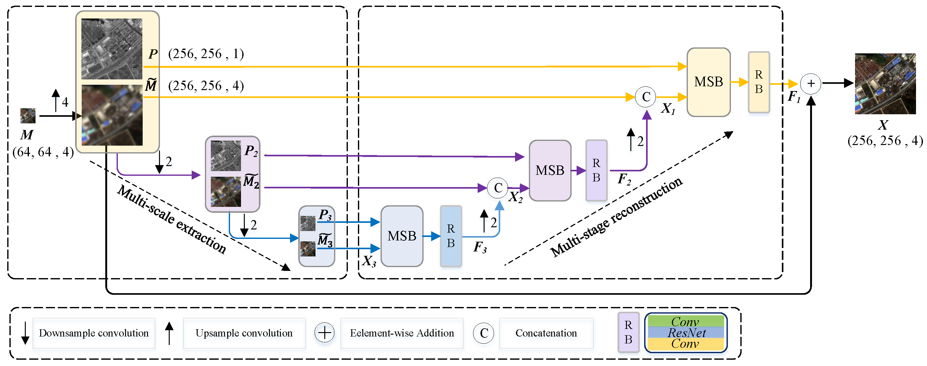
Figure 1. The framework of the multi-scale and multi-stream fusion network (MMFN).
Remotesensing 15 01666 g001
Figure 2. A comparison of three different stream-based fusion blocks. (a) The single-stream block is based on the concatenation of the MS and PAN images. (b) The dual-stream block separately inputs the two source images to the feature extraction network. (c) The multi-stream block (MSB) exploits three streams to separately extract the features from the PAN, the MS, and the concatenation of the two inputs (i.e., MS and PAN). © refers to the concatenation operation.
Remotesensing 15 01666 g002
Figure 3. Qualitative comparison at reduced resolution on the QuickBird dataset. (a) Inter23, (b) AWLP, (c) BDSD, (d) GSA, (e) MMP, (f) MGH, (g) SIRF, (h) PNN, (i) PanNet, (j) PSGAN, (k) ResTFNet- l 1 , (l) TACNN, (m) MUCNN, (n) MMFN, (o) Ground-Truth (GT). The last two rows are MAEs between pansharpened results and the related ground-truth images.
Remotesensing 15 01666 g003
Figure 4. Qualitative comparison at reduced resolution on the Pléiades dataset. (a) Inter23, (b) AWLP, (c) BDSD, (d) GSA, (e) MMP, (f) MGH, (g) SIRF, (h) PNN, (i) PanNet, (j) PSGAN, (k) ResTFNet- l 1 , (l) TACNN, (m) MUCNN, (n) MMFN, (o) Ground-Truth (GT). The last two rows are MAEs between pansharpened results and the related ground-truth images.
Remotesensing 15 01666 g004
Figure 5. Qualitative comparison at reduced resolution on the WorldView-2 dataset. (a) Inter23, (b) AWLP, (c) BDSD, (d) GSA, (e) MMP, (f) MGH, (g) SIRF, (h) PNN, (i) PanNet, (j) PSGAN, (k) ResTFNet- l 1 , (l) TACNN, (m) MUCNN, (n) MMFN, (o) Ground-Truth (GT). The last two rows are MAEs between pansharpened results and the related ground-truth images.
Remotesensing 15 01666 g005
Figure 6. Qualitative comparison at full resolution on the QuickBird dataset. (a) Inter23, (b) AWLP, (c) BDSD, (d) GSA, (e) MMP, (f) MGH, (g) SIRF, (h) PNN, (i) PanNet, (j) PSGAN, (k) ResTFNet- l 1 , (l) TACNN, (m) MUCNN, (n) MMFN (Our). The last two rows are MAEs between the pansharpened results and the Inter23 outcome.
Remotesensing 15 01666 g006
Figure 7. Qualitative comparison at full resolution on the Pléiades dataset. (a) Inter23, (b) AWLP, (c) BDSD, (d) GSA, (e) MMP, (f) MGH, (g) SIRF, (h) PNN, (i) PanNet, (j) PSGAN, (k) ResTFNet- l 1 , (l) TACNN, (m) MUCNN, (n) MMFN (Our). The last two rows are MAEs between the pansharpened results and the Inter23 outcome.
Remotesensing 15 01666 g007
Figure 8. Qualitative comparison at full resolution on the WorldView-2 dataset. (a) Inter23, (b) AWLP, (c) BDSD, (d) GSA, (e) MMP, (f) MGH, (g) SIRF, (h) PNN, (i) PanNet, (j) PSGAN, (k) ResTFNet- l 1 , (l) TACNN, (m) MUCNN, (n) MMFN (Our). The last two rows are MAEs between the pansharpened results and the Inter23 outcome.
Remotesensing 15 01666 g008
Figure 9. Quantitative fusion results by varying the number of scales on the three real remote sensing datasets.
Remotesensing 15 01666 g009
Figure 10. Pansharpening results by using a different number of scales on the three real remote sensing datasets. From top to bottom: fusion results using one, two, and three scales, respectively, and the ground-truth images. From left to right: (a) QuickBird dataset, (b) MAE map of (a), (c) Pléiades dataset, (d) MAE map of (c), (e) WorldView-2 dataset, and (f) MAE map of (e).
Remotesensing 15 01666 g010
Figure 11. Quantitative fusion results by varying the number of streams on the three real remote sensing datasets.
Remotesensing 15 01666 g011
Figure 12. Pansharpening results by using a different number of streams on the three real remote sensing datasets. From top to bottom: fusion results using one, two, and three streams, respectively, and the ground-truth images. From left to right: (a) QuickBird dataset, (b) MAE map of (a), (c) Pléiades dataset, (d) MAE map of (c), (e) WorldView-2 dataset, (f) MAE map of (e).
Remotesensing 15 01666 g012
Figure 13. Quantitative fusion results by varying the number of residual blocks on the three real remote sensing datasets.
Remotesensing 15 01666 g013
Table 1. Parameters of each convolutional layer in the MSB block and RB block.
Layer NameKernel SizeStridePaddingInput ChannelsOutput Channels
Conv03 × 3111 (PAN) or # MS bands (MS)32
Conv13 × 3113264
Conv23 × 3116432
Conv1_13 × 3111 + # MS bands32
ResNet1_13 × 3113232
Conv1_23 × 31132# MS bands
Conv2_13 × 3116432
ResNet2_13 × 3113232
Conv2_23 × 31132# MS bands
Conv(RB)3 × 3112 × # MS bands32
ResNet(RB)3 × 3113232
Conv(RB)3 × 31132# MS bands
Table 2. Average quantitative performance on the QuickBird dataset. The best and second best performances are shown in Red and Blue, respectively.
MethodsCC (1)ERGAS (0) Q 2 n (1)RASE (0)RMSE (0)SAM (0) D λ (0) D S (0)QNR (1)
Inter230.8746 ± 0.06072.2640 ± 0.76060.8599 ± 0.07289.2008 ± 3.310226.4504 ± 11.43060.0388 ± 0.01580.0021 ± 0.00130.0699 ± 0.03030.9282 ± 0.0301
AWLP0.9375 ± 0.03081.5913 ± 0.54950.9346 ± 0.03226.5544 ± 2.492619.1237 ± 10.18740.0304 ± 0.01060.0547 ± 0.03440.0971 ± 0.06990.8558 ± 0.0931
BDSD0.9279 ± 0.03731.8970 ± 0.77290.9211 ± 0.04077.5889 ± 3.262322.0196 ± 12.59660.0374 ± 0.01460.0178 ± 0.01050.0436 ± 0.03260.9394 ± 0.0330
GSA0.9321 ± 0.03821.8597 ± 0.78020.9234 ± 0.04347.3530 ± 3.079621.1029 ± 11.39290.0359 ± 0.01360.0417 ± 0.02720.0974 ± 0.07260.8666 ± 0.0884
MMP0.9385 ± 0.03261.4731 ± 0.58390.9344 ± 0.03675.8352 ± 2.439916.9974 ± 9.75800.0302 ± 0.01120.0209 ± 0.01420.0451 ± 0.04040.9354 ± 0.0481
MGH0.9380 ± 0.03121.6173 ± 0.52300.9358 ± 0.03166.2571 ± 2.146018.2318 ± 9.06960.0297 ± 0.00950.0637 ± 0.03590.1064 ± 0.07090.8391 ± 0.0944
SIRF0.8252 ± 0.10642.4460 ± 0.92310.8007 ± 0.12479.6182 ± 3.865828.3468 ± 16.33640.0511 ± 0.03140.0668 ± 0.04510.0706 ± 0.06740.8687 ± 0.0893
PNN0.9654 ± 0.01751.0973 ± 0.37580.9646 ± 0.017824.3596 ± 1.633512.6981 ± 6.37850.0243 ± 0.00860.0250 ± 0.02690.0527 ± 0.06140.9252 ± 0.0808
PanNet0.9715 ± 0.01250.9736 ± 0.28910.9712 ± 0.01273.8504 ± 1.234111.2352 ± 5.00740.0222 ± 0.00710.0181 ± 0.01880.0208 ±0.02200.9619 ± 0.0384
PSGAN0.9691 ± 0.01561.0041 ± 0.30310.9686 ± 0.01584.0294 ± 1.324811.7302 ± 5.04670.0230 ± 0.00730.0424 ± 0.04880.0545 ± 0.06090.9082 ± 0.0953
ResTFNet- l 1 0.9762 ± 0.01080.8729 ± 0.26160.9758 ± 0.01113.4346 ± 1.101210.0058 ± 4.41440.0203 ± 0.00640.0226 ± 0.02240.0335 ± 0.04690.9456 ± 0.0646
TACNN0.9602 ± 0.02031.1075 ± 0.28620.9589 ± 0.02174.2747 ± 1.166912.3099 ± 4.35650.0254 ± 0.00760.0228 ± 0.02730.0406 ± 0.04710.9387 ± 0.0667
MUCNN0.9700 ± 0.01451.0255 ± 0.36830.9693 ± 0.01504.0755 ± 1.580011.9330 ± 6.52890.0226 ± 0.00780.0206 ± 0.02560.0291 ± 0.04110.9520 ± 0.0619
MMFN (ours)0.9783 ± 0.00990.8368 ± 0.25750.9778 ± 0.01023.3083 ± 1.08349.6204 ± 4.31550.0192 ± 0.00610.0203 ± 0.01720.0273 ± 0.03140.9535 ± 0.0455
Table 3. Average quantitative performance on the Pléiades dataset. The best and second best performances are shown in Red and Blue, respectively.
MethodsCC (1)ERGAS (0) Q 2 n (1)RASE (0)RMSE (0)SAM (0) D λ (0) D S (0)QNR (1)
Inter230.9247 ± 0.03444.0650 ± 1.07260.9178 ± 0.040316.4545 ± 3.314393.9909 ± 23.93160.0554 ± 0.01540.0007 ± 0.00060.0871 ± 0.03660.9122 ± 0.0368
AWLP0.9402 ± 0.02404.0773 ± 0.88030.9376 ± 0.024418.6537 ± 4.3317106.7633 ± 29.14440.0666 ± 0.02890.0354 ± 0.01820.0863 ± 0.04050.8821 ± 0.0538
BDSD0.9154 ± 0.03405.0235 ± 1.62170.9069 ± 0.039720.0637 ± 4.1547113.9981 ± 26.71710.0777 ± 0.02410.0133 ± 0.00720.0628 ± 0.01530.9247 ± 0.0158
GSA0.9282 ± 0.03444.8284 ± 1.74080.9173 ± 0.044419.6190 ± 4.6651111.9132 ± 31.08640.0705 ± 0.02390.0610 ± 0.02690.1637 ± 0.05050.7864 ± 0.0671
MMP0.9363 ± 0.03103.7855 ± 1.11540.9353 ± 0.032215.2021 ± 3.142586.6501 ± 21.49390.0601 ± 0.02080.0077 ± 0.00310.0243 ± 0.02980.9682 ± 0.0296
MGH0.9382 ± 0.02384.2363 ± 1.39040.9338 ± 0.025017.2398 ± 3.779497.8060 ± 22.39850.0531 ± 0.01460.0409 ± 0.02050.0958 ± 0.03960.8680 ± 0.0545
SIRF0.9499 ± 0.02713.1350 ± 0.49130.9474 ± 0.030512.5454 ± 1.772371.7516 ± 14.59130.0595 ± 0.01560.0195 ± 0.01460.0874 ± 0.04420.8964 ± 0.0536
PNN0.9824 ± 0.00821.9860 ± 0.59740.9821 ±0.00848.2626 ± 2.061247.1546 ± 13.79180.0406 ± 0.01200.0286 ± 0.01700.0734 ± 0.03300.9006 ± 0.0465
PanNet0.9876 ± 0.00761.6766 ± 0.72280.9873 ± 0.00817.0452 ± 2.511239.6260 ± 12.82930.0357 ± 0.01120.0167 ± 0.01430.0289 ± 0.01540.9551 ± 0.0283
PSGAN0.9922 ± 0.00391.2959 ± 0.32530.9921 ± 0.00405.4914 ± 1.174431.1803 ± 7.37580.0305 ± 0.00860.0258 ± 0.02080.0736 ± 0.02580.9029 ± 0.0424
ResTFNet- l 1 0.9923 ± 0.00401.2974 ± 0.32510.9922 ± 0.00405.5191 ± 1.180131.4281 ± 7.88120.0302 ± 0.00850.0194 ± 0.01590.0514 ± 0.01530.9304 ± 0.0284
TACNN0.9871 ± 0.00551.7147 ± 0.38560.9870 ± 0.00567.4884 ± 1.436342.7377 ± 10.04000.0417 ± 0.01100.0195 ± 0.01580.0587 ± 0.02440.9233 ± 0.0377
MUCNN0.9896 ± 0.00531.5371 ± 0.53080.9893 ± 0.00566.5236 ± 1.915237.2740 ± 12.63120.0338 ± 0.01000.0165 ±0.01570.0229 ±0.01690.9611 ± 0.0311
MMFN (ours)0.9930 ± 0.00371.2197 ± 0.32770.9930 ± 0.00375.1791 ± 1.122529.3613 ± 6.90010.0281 ± 0.00800.0173 ± 0.01230.0223 ± 0.00960.9609 ± 0.0189
Table 4. Average quantitative performance on the WorldView-2 dataset. The best and second best performances are shown in Red and Blue, respectively.
MethodsCC (1)ERGAS (0) Q 2 n (1)RASE (0)RMSE (0)SAM (0) D λ (0) D S (0)QNR (1)
Inter230.8729 ± 0.06024.0245 ± 1.90830.8588 ± 0.071115.4794 ± 7.745553.3841 ± 25.84460.0515 ± 0.02310.0035 ± 0.00500.0545 ± 0.03330.9423 ± 0.0370
AWLP0.9307 ± 0.04282.9811 ± 1.84520.9283 ± 0.044212.8921 ± 7.029743.5665 ± 17.82910.0484 ± 0.02010.0640 ± 0.06530.0833 ± 0.08450.8629 ± 0.1236
BDSD0.9248 ± 0.05033.2997 ± 2.23020.9213 ± 0.051712.9515 ± 8.281543.3519 ± 20.50320.0566 ± 0.02690.0347 ± 0.03420.0456 ± 0.04260.9224 ± 0.0657
GSA0.9301 ± 0.05423.2834 ± 2.64870.9239 ± 0.058512.8705 ± 9.482242.4991 ± 22.83620.0559 ± 0.03030.0621 ± 0.06020.1165 ± 0.10150.8335 ± 0.1330
MMP0.9393 ± 0.04372.6916 ± 1.89410.9331 ± 0.048610.8338 ± 6.997636.3995 ± 17.66180.0467 ± 0.02350.0269 ± 0.01390.0386 ± 0.02750.9357 ± 0.0353
MGH0.9359 ± 0.04173.0157 ± 2.00170.9340 ± 0.042511.9062 ± 7.263239.9244 ± 17.55110.0451 ± 0.01970.0689 ± 0.06140.0900 ± 0.08180.8519 ± 0.1187
SIRF0.8431 ± 0.15784.7626 ± 1.88490.8091 ± 0.162418.5698 ± 9.000562.0451 ± 22.79930.1146 ± 0.07840.1013 ± 0.08230.0873 ± 0.08010.8263 ± 0.1377
PNN0.9659 ± 0.02671.8580 ± 0.95840.9649 ± 0.02787.5961 ± 3.732426.0741 ± 11.57820.0360 ± 0.01810.0340 ± 0.05970.0534 ± 0.06490.9178 ± 0.1024
PanNet0.9704 ± 0.02571.6760 ± 0.76250.9696 ± 0.02676.8436 ± 2.979623.6430 ± 10.03500.0330 ± 0.01510.0395 ± 0.05390.0547 ± 0.07200.9115 ± 0.1105
PSGAN0.9703 ± 0.02751.6735 ± 0.75200.9694 ± 0.02866.7857 ± 2.953023.4621 ± 10.20500.0322 ± 0.01460.0454 ± 0.07160.0533 ± 0.07430.9084 ± 0.1205
ResTFNet- l 1 0.9722 ± 0.02621.5961 ± 0.72760.9716 ± 0.02726.5399 ± 2.857122.6806 ± 10.01960.0309 ± 0.01410.0376 ± 0.06930.0411 ± 0.06670.9271 ± 0.1133
TACNN0.9562 ± 0.03332.2537 ± 0.97030.9537 ± 0.03799.1814 ± 3.408930.9212 ± 9.90470.0440 ± 0.01720.0344 ± 0.04420.0379 ± 0.04640.9309 ± 0.0800
MUCNN0.9694 ±0.02561.7244 ± 0.82900.9685 ± 0.02687.0707 ± 3.225124.4422 ±10.74360.0332 ± 0.01560.0305 ± 0.05480.0354 ± 0.05760.9381 ± 0.0963
MMFN (ours)0.9753 ± 0.02261.5102 ± 0.67500.9746 ± 0.02376.1888 ± 2.646121.4883 ± 9.42220.0291 ± 0.01320.0332 ± 0.07160.0348 ± 0.06750.9379 ± 0.1137
Table 5. Parameter numbers and running times for the compared deep learning methods on datasets at different scales.
MethodsScale (Time)# Parameters
RR (s)FR (s)
PNN0.141.6780,420
PanNet0.263.8421,384
PsGan1.1113.772,367,716
ResTFNet- l 1 0.8512.002,362,869
TACNN0.151.7280,420
MUCNN0.517.211,362,832
MMFN (ours)0.628.97328,142
Disclaimer/Publisher’s Note: The statements, opinions and data contained in all publications are solely those of the individual author(s) and contributor(s) and not of MDPI and/or the editor(s). MDPI and/or the editor(s) disclaim responsibility for any injury to people or property resulting from any ideas, methods, instructions or products referred to in the content.