Abstract
In this work, a dedicated campaign by MetOp-A satellite is conducted to monitor the ionosphere based on radio-occultation (RO) measurements provided by the onboard GNSS (Global Navigation Satellite System) Receiver for Atmospheric Sounding (GRAS). The main goal is to analyze the capabilities of the collected data to represent the bending angle and scintillation profiles of the ionosphere. We compare the MetOp-A products with those generated by other RO missions and explore the spatial/temporal distributions sensed by the MetOp-A campaign. Validation of dual frequency bending angles at the RO tangent points, S4 index, and Rate of the Total electron content Index (ROTI) is performed against independent products from Fengyun-3D and FORMOSAT-7/COSMIC-2 satellites. Our main findings constitute the following: (1) bending angle profiles from MetOp-A agree well with Fengyun-3D measurements; (2) bending angle distributions show a typical S-shape variation along the altitudes; (3) signatures of the sporadic E-layer and equatorial ionization anomaly crests are observed by the bending angles; (4) sharp transitions are observed in the bending angle profiles above ~200 km due to the transition of the daytime/nighttime in addition to the transition of the bottom-side/top-side; and (5) sporadic E-layer signatures are observed in the S4 index distributions by MetOp-A and FORMOSAT-7/COSMIC-2, with expected differences in magnitudes between the GPS (Global Positioning System) L1 and L2 frequencies.
Keywords:
GNSS; GPS; MetOp; radio-occultation; ionosphere; space weather; S4 index; sporadic E-layer; COSMIC; Fengyun 1. Introduction
GNSS Radio-Occultation (RO) as a technique to measure the Earth’s ionosphere [1] was first applied to the GPS/MET satellite mission in the 1990s [2,3]. Several Low Earth Orbit (LEO) satellites carrying onboard GNSS receivers were later used to further explore the ionosphere. Early examples of RO satellite missions include CHAMP [4], SAC-C [5], and the Formosa Satellite 3/Constellation Observing System for Meteorology, Ionosphere, and Climate (FORMOSAT-3/COSMIC) [6]. Currently, thousands of ionospheric RO measurements are daily obtained by different data providers. Well-known missions are the FORMOSAT-7/COSMIC-2 [7,8], operated by the University Corporation for Atmospheric Research (UCAR), Spire [9], a commercial operator, and Fengyun [10], operated by the National Satellite Meteorological Center (NSMC) of the Chinese meteorological administration. More recently, the MetOp satellite mission, operated by the European Organization for the Exploitation of Meteorological Satellites (EUMETSAT), also provided GNSS RO measurements to explore the ionosphere.
The MetOp-A satellite was launched in October 2006 as the first European polar-orbiting satellite dedicated to meteorology. With an array of several instruments, it was initially designed for global weather forecasting and climate monitoring, providing, e.g., temperature, humidity, wind speed, and ozone parameters. As part of the MetOp payload, the onboard GNSS Receiver for Atmospheric Sounding (GRAS) is dedicated to acquiring GNSS limb-sounding measurements for atmospheric profiling and precise orbit determination [11]. The main objective of the occultations is to provide stratospheric and tropospheric temperature and humidity information to be assimilated in Numerical Weather Prediction (NWP) models. The measurements are therefore provided to describe the lower atmosphere. In 2020, however, during an end-of-life testing campaign of the MetOp-A satellite mission, EUMETSAT enabled the GRAS instrument to extend its vertical measurement range up to 300 and 600 km height in two different experiments. Although the satellite was flying at around 800 km, the received signal was truncated in the upper atmosphere, neglecting the data above 300 km and 600 km. The goal of this campaign was to test the ionosphere monitoring capabilities of the GRAS receiver by validating the ionospheric products (dual frequency bending angle and scintillation index profiles) and minimizing the impact of the vertical range extension over the neutral atmospheric products. Aiming to explore these unique measurements, a dedicated study was launched by EUMETSAT to evaluate the quality of these ionospheric products against similar products independently generated by other processing centers, with a particular interest in the Fengyun 3D and FORMOSAT-7/COSMIC-2 (or COSMIC-2 in short) missions.
The GNSS radio-occultation measurements collected during the end-of-life experimental campaign of MetOp-A covered a three-month period during the Northern hemisphere summer of 2020. The dataset consists of high-resolution (50 Hz) dual frequency amplitude and phases collected by the fore-and-aft antennas of the GRAS receiver during rising and setting occultations, respectively. Within the GRAS ionospheric measurements, this work analyzes the processed dual frequency bending angle and scintillation profiles. The main goal is to compare the GRAS profiles against other RO mission measurements and explore the main ionospheric dynamics observed during the campaign. Usually, GNSS RO measurements are validated against external data sources. Ionosonde stations and incoherent scatter radars, for instance, are commonly used as a reference to the validation [12,13,14,15,16,17,18,19,20,21,22] since they provide accurate observations of the electron density. In-situ measurements provided by external satellite missions are also extensively used to assess the RO measurements [23,24,25,26,27,28,29,30]. Another typical evaluation metric is to compare the RO observations against climatological models of the ionosphere [31,32,33,34,35]. Most of these validation techniques, however, require deriving the electron density values from the carrier phase and pseudo-range measurements. A validation in terms of electron density data observed by MetOp-A is provided by [36]. In the present work, we carry out the validation directly over the bending angle [37,38] and signal fading observations [39,40,41], providing additional validation over the MetOp-A dataset. Details of the dataset collected by the MetOp-A satellite and other RO missions used for comparisons are presented in Section 2. Section 3 and Section 4 show the results regarding the bending angles and scintillation profiles, respectively. The final conclusions are given in Section 5.
2. Materials and Methods
2.1. Dataset
The GRAS dataset released by EUMETSAT refers to the days of the year (DOY) 176 to 253 of 2020, which corresponds from 24 June up to 9 September. The dataset was produced by updating the standard near-real-time processor of EUMETSAT that provides RO L1b products to the NWP centers. This update allowed us to extend the dual frequency bending angle profiles (available in the standard product in the neutral atmosphere only) to cover the entire GRAS measurement range (up to 300 or 600 km depending on the experiment). It also enabled us to include dual frequency profiles of amplitude and phase scintillation indexes at a high rate. The product, one file per each measured occultation, includes high-rate raw observations, i.e., dual frequency excess phases and signal amplitudes. It must be noted that the excess phases represent the phases in excess with respect to the vacuum propagation, i.e., it is obtained by removing the geometry (the straight-line distance between the transmitter and receiver) from the measured carrier phases. Additionally, the MetOp-A and GNSS satellite orbits and clocks trimmed for each individual occultation are released in the products.
To perform validation with independent data, two other RO satellite missions providing similar ionospheric data are selected: Fengyun-3D (FY-3D) and COSMIC-2. The FY-3D data were obtained through the China meteorological administration of the NSMC via the portal http://satellite.nsmc.org.cn/ (accessed on 1 November 2021). Such a dataset includes bending angle measurements at the L1 frequency and the associated electron density profiles. The COSMIC-2 data processed by UCAR was instead obtained through the COSMIC Data Analysis and Archive Center (CDAAC) via the portal https://data.cosmic.ucar.edu/ (accessed on 1 November 2021). The data referred to in the level 1b archive were used to provide TEC and S4 measurements per each occultation observed by the COSMIC-2 GNSS receivers.
2.2. Parameters Used for the Validation
Four parameters are used to analyze and validate the data retrieved by the GRAS measurements collected onboard MetOp-A. They constitute the following:
- Bending angle in the L1 GPS frequency;
- S4 in the L1 GPS frequency;
- S4 in the L2 GPS frequency;
- Rate of TEC index (ROTI).
Assuming the refractive index as spherically distributed around the tangent points of a radio-occultation event, the bending angle α (the overall bending of the ray path caused by the atmospheric refraction) at the impact parameter (the distance of the asymptotes of the ray path from the Earth’s center) is given by the following Abel integral:
where is the refractive index, and is the variable associated with the impact parameter integration. This integral, once inverted, can be used to retrieve the atmospheric refractivity profile which, in turn, can be used to infer the vertical distribution of temperature, pressure, and water vapor in the neutral atmosphere as well as the vertical distribution of electron density in the ionosphere. The basic principles of this radio-occultation technique can be found in Kursinski et al. [1]. The main assumption in Equation (1) is that the refractivity fields are spherically distributed. Another assumption is that the upper limit of the Abel integral is set at an altitude where the refractive index is supposed to be 1. To process the GRAS ionospheric measurements, which are taken only up to 300 km or 600 km, an ad hoc implementation, including the Abel inversion to derive electron density profiles, is used [36]. Then, the ionospheric bending angles are derived by the Doppler-shift measurements following a Geometrical Optics approach. It is well known that the Wave Optics approach [42] improves drastically the neutral bending angle retrieval in the troposphere, where the gradients introduced by water vapor distribution might cause super-refractive layers and even ducting in tropical regions. When this occurs, radio-occultation measurements suffer stronger atmospheric-induced multipath. Multiple signals following different paths and characterized by different impact parameters are contemporaneously received, making the Geometric Optics assumption invalid. On the other hand, it is well known that Wave and Geometric Optics approaches provide similar results when the atmospheric multipath can be neglected, which is mostly the case in the ionosphere. Given that the Geometric Optics approach reduces the computational burden and that the main goal of this study is to show a general picture of the bending angle derived from the high-rate GRAS measurements, we adopted the simpler Geometrical Optics approach.
The S4 index is a measure of amplitude scintillation caused by a severe drop in the C/N0 received by GNSS signals, which is typically used to infer ionospheric irregularities. It occurs differently in GPS L1 and L2 measurements and is defined as the ratio between the standard deviation of the signal’s intensity over its mean intensity [43]:
where the signal intensity is calculated from the in-phase and quadrature-phase component outputs of the central correlator. The brackets in Equation (2) denote an average over a fixed integration time equal to 1 s. Differently from a ground-based geometry, the space-based RO signals are emerging from the ionospheric limb and are quickly spanning the ionospheric irregularities in the vertical direction. The derived S4 values are therefore a representation of the irregularities over the entire RO ray path, despite being usually mapped at the tangent points. As shown by Wu [44], disturbances in the E- and F-layers can affect the lower atmosphere due to the slant view geometry of the measurements and the tilt angle of the disturbances. However, in the current work, only the ionosphere above the E-layer is studied. As a result, ionospheric S4 profiles are analyzed considering the main source of irregularities at the tangent points. A detailed analysis of the observed S4 profiles is presented in Section 4.
Another metric commonly used to analyze the ionospheric scintillations is the rate of change of TEC (ROT) [45]. It can be used to describe the phase fluctuations and is obtained based on the following equation:
where is the slant TEC and the sample rate is chosen as 1 s.
We extracted the directly from the RO excess phase measurements, avoiding the need for differential code bias (DCB) calibration. In this sense, the values are computed by the following:
with
where and are the excess phase measurements for the L1 and L2 frequencies, respectively.
The standard deviation of , termed the rate of TEC index (), can usually be adopted as a better proxy for a scintillation event than . The expression is computed in a similar way to the common . As shown by [46], it is given as follows:
where ⟨ ⟩ represents the sliding average value over a certain time interval. Usually, the is computed using a 5-min sliding window; however, this is mainly applied to ground-based GNSS observations. The GNSS signal geometry changes very slowly when observed by ground-based receivers. In the case of the present work, satellite-based observations from MetOp-A or COSMIC-2 are used. Since the GNSS signal geometry changes much faster when observed by satellite-based receivers, we selected a smaller time window. Empirically, we selected a 10 s sliding window.
3. Study of RO Bending Angles
The assessment of the RO bending angles derived by MetOp-A observation is performed using the FY-3D data as a reference. Figure 1 shows the differences in the orbits of both missions during arbitrarily selected days from the dates of interest. Each dot represents all the Tangent Points (TPs) used to geolocate the individual ionospheric profiles in terms of latitude and Local Time (LT). As we can see, most of the observation points are in the polar regions. In the other regions, the FY-3D profiles (see black dots) are obtained with a different LT pattern than those from MetOp-A. Due to this difference, we perform a quantitative assessment considering only collocated profiles, mostly occurring in the high latitudes. The results with the collocated data are shown in Section 3.1. Additionally, Section 3.2 presents an analysis of the entire dataset, using non-collocated data. This is performed to explore the latitude and LT dependencies obtained by both satellite mission data, which is not possible with the collocated dataset.
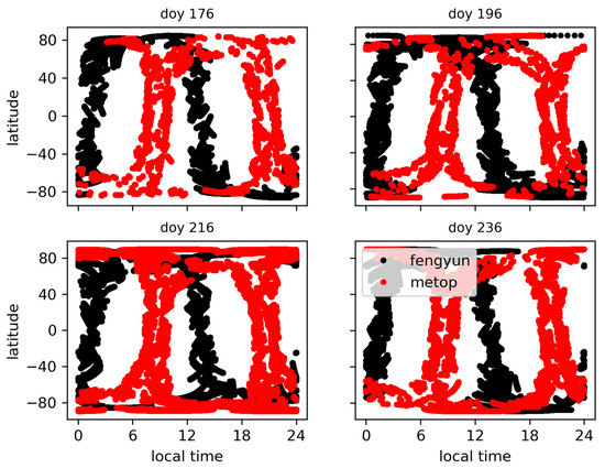
Figure 1.
Local time pattern of the tangent points observed by the MetOp-A (see red dots) and FY-3D satellite. Each panel shows the footprint of the tangent points for specific DOYs of 2020.
3.1. Collocated Profiles
Figure 2 shows some examples of bending angle profiles obtained by MetOp-A and FY-3D when they are collocated. The collocation is performed assuming that the whole ionospheric profile can be geolocated at a certain location, selected as the latitude and longitude position of the tangent point between the straight line connecting the two satellites. For each profile, one from MetOp-A and the other from FY-3D, we check if the corresponding latitudes, longitudes, and times of these two positions are within a certain threshold. A broad area threshold is assumed with 2.5° × 2.5° in latitude by longitude, and a time window is set as two hours. As Figure 2 shows, the FY-3D and MetOp-A bending angle profiles are quite similar. They all show a similar exponential increase up to ~200 km, followed by a decrease above ~200 km. In case these profiles are converted to electron density values, the peak height (hmF2) would be close to 200 km. This occurs because the bending angle has a linear correlation with the derivative of the electron density, i.e., the electron density inversion point of an ionospheric profile occurs where the bending angle is closer to zero. A difference to be highlighted in this example is that the MetOp-A profile is truncated at ~250 km, whereas the FY-3D data goes up to ~500 km. Although MetOp-A was flying at an orbit height of about 800 km, the GRAS instrument was developed mainly to observe the lower atmosphere, so the measurements were truncated in higher altitudes. In these examples, the FY-3D profiles are intentionally truncated to ~300 km for better visualization. Additionally, the FY-3D profile data points present a lower resolution than the MetOp-A data.
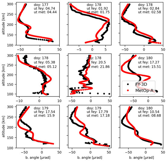
Figure 2.
Bending angle profiles at GPS L1 frequency from MetOp-A (red curve) and Fengyun 3D (black curve) when considering a collocation of 2.5 × 2.5 deg in latitude and longitude. The time collocation is 2 h, i.e., the maximum time difference between MetOp-A and Fengyun 3D is 2 h for all the points in a specific profile.
Another example of profiles is presented in Figure 3, however, assuming a time collocation of 4 h. The agreement in this case is worse. The difference between using 2 and 4 h in the time collocation period becomes even more evident when looking at the statistics shown in Figure 4. These results show the mean and standard deviation of the difference considering all the collocated bending angle profiles collected between DOYs 176 and 253 of 2020. The mean difference between MetOp-A and FY-3D has a sinusoidal pattern associated with the sinusoidal pattern of the bending angle profiles. Overall, the mean difference is centered around zero, so no clear bias is observed between the datasets of the two missions. In the case of the 4 h collocation, the differences become more evident at the E-layer peak height (around 110 km) and at the F2-layer peak height (around 230 km). This is expected since these are the regions with the highest variability in the ionosphere. In the case of the 2 h collocation, the standard deviation of the difference is quite constant over the altitudes with a magnitude of about 10 µrads. The magnitude of the standard deviation using a 4 h collocation varies between 10 to 40 µrads. Therefore, as we improve the collocation time of the measurements, we obtain a better agreement. Assuming an ideal case, where the observations are taken at the same TP positions, we can expect a lower standard deviation. This provides evidence that the MetOp-A and FY-3D bending angles are consistent.
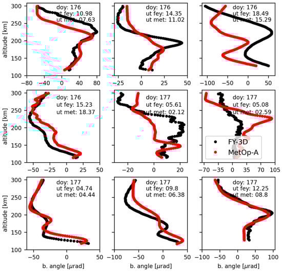
Figure 3.
Bending angle profiles at GPS L1 frequency from MetOp-A (black curve) and Fengyun 3D (red curve) when considering a collocation of 2.5 × 2.5 deg in latitude and longitude. The time colocation is 4 h, i.e., the maximum time difference between MetOp-A and Fengyun 3D is 4 h for all the points in a specific profile.
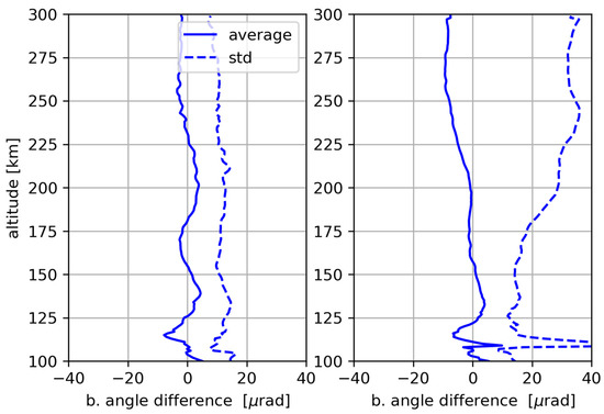
Figure 4.
Mean and standard deviation of the difference between the bending angle profiles at GPS L1 frequency from MetOp-A and Fengyun 3D when considering the entire dataset (DOYs 176 to 253). The collocation is assumed with 2.5° × 2.5° in latitude and longitude, 2 h in time for the left panel, and 4 h in the right panel.
3.2. Non-Collocated Profiles
The analysis using non-collocated profiles is performed to evaluate the overall distributions within the latitudes, altitudes, and local times. Figure 5, for instance, shows the profile distributions over altitude, where the entire dataset of the measurements during DOYs 176 to 253 of 2020 is used. The distribution shows the number of occurrences of a specific bending angle value divided by the maximum number of occurrences at the specific height. It can be understood as a two-dimensional histogram binned with 1 µrad by 2 km. The hot color, therefore, shows the region with the highest agglomeration of bending angles. As shown, both distributions (MetOp-A and FY-3D) are very similar. They both show an S-shape variability, with the lowest values close to 225 km. There is also a peak in the E-layer region around 100 km clearly shown in MetOp-A and a bit noisy in FY-3D, which is likely related to the sporadic E-layer.
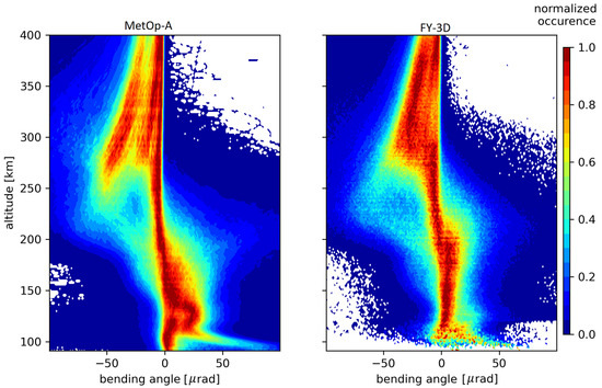
Figure 5.
Altitude distribution of the bending angle values at L1 derived from the MetOp-A measurements (left panel) and Fengyun-3D data (right panel) during the entire collocated dataset (DOYs 176 to 253 of 2020). The color bar shows the normalized occurrence of the most predominant patterns in the dataset. The white background represents the absence of data.
Figure 6 shows the bending angle distributions of MetOp-A and FY-3D in terms of latitude at a given altitude. Again, we use the entire dataset to compute binned values, however, with bins of 1 degree in latitude and 5 km in altitude. The MetOp-A data shows a very reasonable distribution of the bending angle. We can see higher values in the E-layer associated with the sporadic E-layer dynamics, mainly in the equatorial region and in the Northern hemisphere. This pattern is also confirmed by [47,48], and this shows that the sporadic E-layer mainly occurs in the summer and is quite rare in the winter. As mentioned by Niu et al. [47], the difference between the two hemispheres is induced by the difference between the magnetic and geographic latitudes. This is directly affected by the zonal wind shear, which is the mechanism that controls the sporadic E-layer occurrence. In the case of the FY-3D distributions, we can see that no observations are collected in the equatorial region of the E-layer. This absence of data, unfortunately, limits the comparison between the two datasets. However, we can see higher values of bending angles at +80 degrees and small values at −80 degrees, which indicates a similar pattern to the MetOp-A values. Moving up to 200 km, we can see two peaks around −15 and 15 degrees in latitude. These are associated with the Southern and Northern crests of ionization known as the Equatorial Ionization Anomaly (EIA). It is relevant to notice that the FY-3D crests are more elevated than the MetOp-A crests. This mainly occurs because the passage of the FY-3D satellite in the equatorial region coincides with the daily peak at around 15 h LT (see Figure 1). In the case of MetOp-A, the satellite passage in the equatorial region is around 09:30 or 20:00 h LT, when the vertical drift of the ionosphere is significantly reduced.
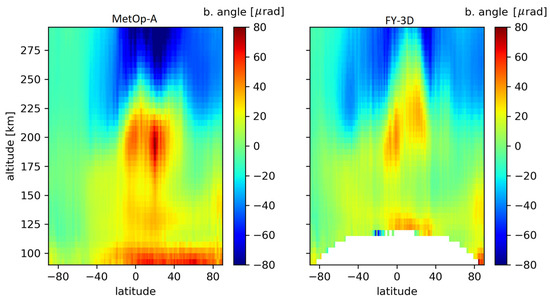
Figure 6.
Bending angle distribution at L1 frequency in terms of altitude by latitude from the MetOp-A measurements (left panel) and Fengyun-3D data (right panel).
Figure 7 shows the bending angle height variation as a function of local time. The averages are computed using bins of 0.5 h in local time and 5 km in altitude. As expected, the highest values from MetOp-A in the E-layer occur in the daytime, due to the previously mentioned dominance of the sporadic E-layer. In the case of the FY-3D data, the E-layer distributions are scattered, which is reasonable due to the absence of data in the equatorial region, as shown in Figure 6 (right panel). Between 125 and 200 km, the FY-3D distribution differs quite strongly from the MetOp-A data, having maximums between 12 and 18 LT. This is expected since the FY-3D passage in the equatorial region is around 15 LT while MetOp-A passes over the equator after 18 h LT. We also see higher values in MetOp-A in the F-layer after 18 h LT. Indeed, the maximum positive values are typically around 125 km. This distribution uplifts to around 175 km shortly after 18:00 LT due to the pre-reversal enhancement period [49]. The electron density peak height (i.e., hmF2) from MetOp-A is therefore found at higher altitudes after 18:00 LT compared to that in mid and high-latitude regions. In the case of the FY-3D, the satellite does not pass over the equatorial region during the pre-reversal enhancement period. Both graphs of Figure 7 also show a U-shape blue region at higher altitudes in the daytime. This occurs due to the bending angle transition between positive to negative at the peak height. The bending angle has a strong transition in the daytime and a rather weak decrease in the nighttime.
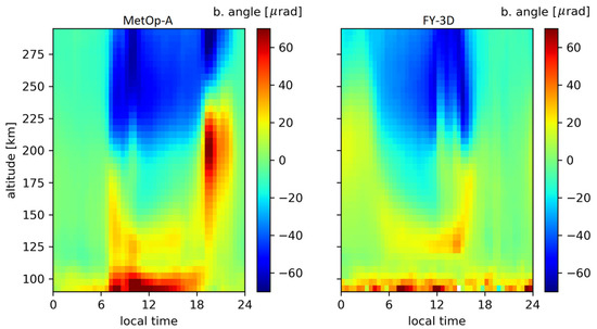
Figure 7.
Bending angle distribution at L1 in terms of altitude by local time from the MetOp-A measurements (left panel) and Fengyun-3D data (right panel).
4. Study of RO Scintillation Profiles
The characteristics of the RO scintillation profiles derived from MetOp-A observations are compared with the COSMIC-2 scintillation data in this section. The analysis is performed considering dual frequency amplitude scintillations profiles. The COSMIC-2 observations are located at different local times and latitudes in comparison to the MetOp-A observations. Figure 8 shows the differences in the LT patterns of both missions on a few dates of interest. As we can see, all the COSMIC-2 observations are concentrated at latitudes of −40 and 40 degrees. The closest locations between MetOp-A and COSMIC-2 measurements occur mainly in low latitudes and around 8 and 20 LT. Due to this distribution, we could not find a significant number of collocated points to compute statistical differences. Only around 12 profiles were well-collocated. Therefore, in this section, we analyze and compare only the LT, latitude, and altitude distributions of the entire dataset, without considering colocation.
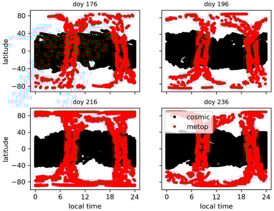
Figure 8.
LT patterns of the tangent (representative measurement) points observed by the MetOp-A and COSMIC-2 satellites. Each panel shows the footprint of the tangent points for specific DOYs in 2020.
To have an initial idea of the S4 distributions, Figure 9 shows two of the most observed patterns of the S4 values by MetOp-A. The left panel is related to the latitude distribution. The right panel is related to the LT distribution. Most of the S4 values observed by the RO geometry depend on the irregularities of the sporadic E-layer. As we can see, the highest S4 values occur at around 100 km, which is an average peak of the E-layer. Sporadic E activity peaks are more pronounced in the summer. Therefore, the seasonal behaviors directly impact the S4 index values. As expected, the highest S4 values are located around +40 degrees in latitude, since the dates of interest relate to the Northern summer. The LT distributions show two maximums near 10:00–13:00 LT and 18:00–23:00 LT. This semi-diurnal variation is generally consistent with ground-based observations from several sites in the Northern hemisphere [50]. Moreover, as shown in Figure 8, MetOp-A crosses the equatorial region shortly after 18:00 h LT. It is well known that amplitude scintillation is more prominent in the equatorial region, especially after sunset hours. Both distributions agree well with previous research conducted by Wu et al. [44,51]. It is worth mentioning that, in this previous work, the LT peaks are found around 08:00–12:00 LT and 18:00–22:00 LT. Here, the LT peaks are near 10:00–13:00 LT and 18:00–23:00 LT, which is justified due to the differences in the satellite orbits.
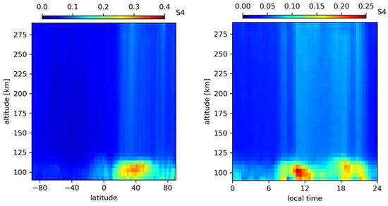
Figure 9.
S4 distribution of the entire dataset (DOYs 176 to 253 of 2020) in terms of latitude (left panel) and LT (right panel) observed by the MetOp-A satellite.
Figure 10 shows a comparison of the S4 values computed by MetOp-A in the GPS L1 and L2 frequencies. Overall, we can see that both distributions are very compatible. The major difference is that the S4 values obtained for L2 signals are higher. As expected, the scales of irregularities detected by the L1 and L2 signals are not the same due to different signal frequencies. As shown by [52,53], the S4 index is higher at L2 frequencies in comparison to the L1 frequency. Based on the relation given by Equation (3) in [52], the S4 values are expected to be 1.45 times higher in the L2 frequency when compared to L1. Our computations revealed maximum values of 0.25 at L1 and 0.4 at L2, showing that the S4 index at L2 is 1.6 times larger than the S4 at L1. On average, we have found a factor of 1.5. This is reasonable since the factor computed here is based on experimental data, i.e., affected by measurement noises, while the relation presented by [52] is theoretical.
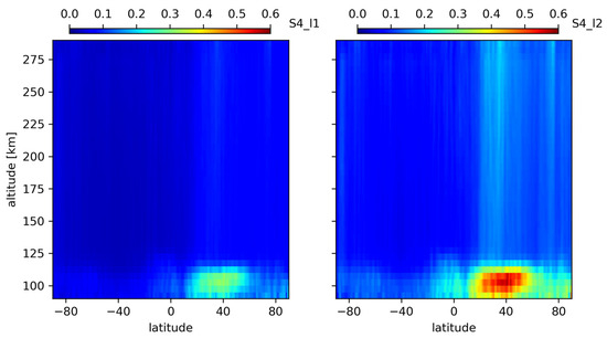
Figure 10.
S4 distribution of the entire dataset (DOYs 176 to 253 of 2020) in terms of altitude by local time from the MetOp-A measurements at L1 (left panel) and L2 (right panel) frequencies.
Figure 11 shows the distribution of the S4 values at the L1 frequency observed by MetOp-A (top panel) and COSMIC-2 (bottom panel) missions as a function of latitude and DOY. Each pixel of Figure 11 is an average of all S4 values measured with a bin of 5 degrees in latitude and 0.1 days, i.e., 2.4 h. The representation is referred to as an altitude of 100 ± 20 km. Figure 12 shows a similar analysis but considers the distribution in terms of latitude by altitude. As can be seen, the MetOp-A S4 index has the highest values around 40 degrees North. As we move towards the equator, the S4 values smoothly decrease until reaching almost zero. There is a sharp decrease of 20 degrees North, where the S4 values vary from 0.2 to zero. As shown by Niu et al. [47], a sharp change in the S4 values is expected at around 20°N latitude at 100 km altitude in the summer. The sudden change of S4 around the 20°N latitude can be explained by the presence of sporadic E-layers, which have a steep boundary on the equator side. The sporadic E-layers observed by the MetOp-A S4 values are mapped at around 100 km, which is coincident with previous studies [22,54,55].
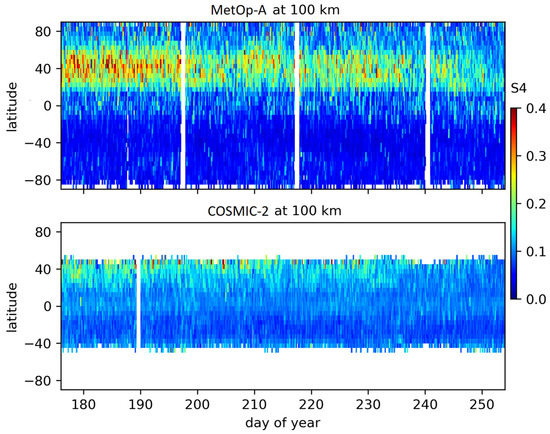
Figure 11.
S4 distribution derived from MetOp-A (top panel) and COSMIC-2 (bottom panel) L1 signal as a function of geographic latitude and day of the year. This graph is generated considering all measurements at 100 ± 20 km. The white background represents the absence of data.
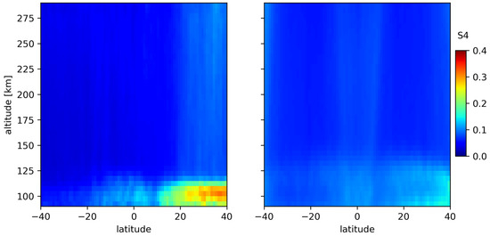
Figure 12.
S4 distribution in terms of altitude by latitude from the MetOp-A measurements at L1 (left panel) and COSMIC-2 measurements at L1 (right panel).
The higher values observed in the Northern hemisphere are related to the Northern summer [22,56]. In the case of the COSMIC-2 data, the observation limitation between −40 and 40 degrees in latitude hampers a proper analysis of the seasonal behavior. However, we can see a slight increase in the S4 values when moving towards 40 degrees North. It is also possible to notice that the COSMIC-2 S4 values are slightly larger in the low latitudes in comparison to the MetOp-A distributions. This difference is also justified since we are not considering collocated measurements in the representation, so the satellites are passing through distinct local times and longitudes, mainly at the equator. Another point is that the estimated S4 index may also depend on the measuring instrument electronics. An ideal comparison is only possible when two missions use the same receiver types. However, this is not the case for MetOp-A and COSMIC-2 missions. COSMIC-2 uses the tri-band GNSS receiver system developed by NASA/JPL capable of receiving and processing signals from GPS, Galileo, and GLONASS systems. MetOp-A uses the GRAS receiver system developed by RUAG, capable of receiving and processing only GPS signals.
To have a similar view of the scintillation distributions between MetOp-A and COSMIC-2 while minimizing the problem due to different GNSS receivers, Figure 13 shows ROTI profiles observed in terms of altitude and local time. Again, the measurements are not collocated. The averages are computed using bins of 0.5 h in local time and 5 km in altitude. In this case, there are several similarities between the distributions over the distinct altitudes and local times. We can clearly see the presence of sporadic E-layers and EIA crests at the times the satellites are passing through the equator. It is relevant to notice that the magnitude of the ROTI values among the missions is more similar when compared to the S4 values, varying up to 4.5 × 10¹⁵ TEC/s in both COSMIC-2 and MetOp-A datasets. Differences are evident in the post-sunset E-layer, where we can see higher values by MetOp-A, reaching ~1.8 × 10¹⁵ TECU/s, while the COSMIC-2 ROTI values are lower, reaching ~0.9 × 10¹⁵ TECU/s. As explained before, these differences are mostly related to the different orbit geometries.
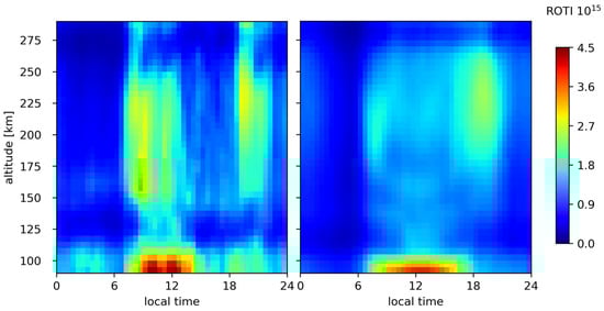
Figure 13.
Distribution in terms of altitude by local time of ROTI measurements at L1 from MetOp-A (left) and COSMIC-2 (right). Values shown here are not co-located. MetOp-A values are computed from −40 to 40 degrees to better match the COSMIC distribution. The unit of the color bar is TECU/s.
5. Conclusions
This study analyzed the distribution of different ionospheric parameters given by MetOp-A radio-occultation measurements and compared them to parameters observed by FY-3D and COSMIC-2 missions. The following conclusions are outlined:
- The collocated assessment showed agreement between the MetOp-A and FY-3D datasets in terms of the bending angle measurements. No bias was found between the bending angles. The standard deviation of the differences between the missions reduces as the observations are closer in space and time.
- FY-3D and MetOp-A bending angle distributions show clear similarities. They both show an S-shape variation within the altitudes with the lowest values close to 225 km in altitude. A peak in the E-layer region around 100 km, related to the sporadic E-layer, is also observed in both datasets in the Northern hemisphere. Above 200 km, two peaks, around −15 and 15 degrees, were observed by the GRAS receiver onboard MetOp-A. These are associated with the impact of the EIA crests on the bending angles. In the case of FY-3D, the EIA crests are more elevated because the passage of the FY-3D satellite in the equatorial region occurs when the vertical drift is enhanced, while the MetOp-A passage in the equatorial region occurs when the vertical drift of the ionosphere is reduced. A U-shape distribution was observed in both missions, with a sharp decrease in altitude of the bending angle during the daytime at the F-layer, and a flat variation of the bending angle at night.
- In the case of scintillations, we observed similar S4 distributions between the GPS L1 and L2 frequencies, with a difference in the S4 magnitude. The S4 values were about 1.5 times higher in L2 than in L1, which agrees well with the previous literature. An external assessment was not applied to collocated measurements due to the misalignment of the orbital locations between COSMIC-2 and MetOp-A. As in the bending angle analysis, we could find clear evidence of sporadic E-layer-induced effects. Previous literature studies have shown that the presence of a sporadic E-layer is the main source of RO scintillation over the middle latitude region, which is confirmed by our study.
- The magnitude of the ROTI values varies up to ~4 × 10¹⁵ TECU/sec in both COSMIC-2 and MetOp-A datasets, having clear LT and altitude dependencies. It was possible to detect the occurrence of sporadic E-layers and clear signatures of irregularities in the F-layer during the post-sunset hours, likely associated with vertical drifts.
A main limiting factor of the current study is that only three months of data were available. This has restricted the number of profiles collocated with other missions and impacted the statistics computed in the MetOp-A assessment. Additionally, our investigation is restricted to the Northern summer of 2020. It would be relevant to extend the analysis and understand the bending angle and scintillation distributions over distinct seasons and solar activities. Hence, in the future, it is planned to extend the MetOp dataset campaign to provide near real-time RO data on the ionosphere obtained by the GRAS instrument. The data evaluation presented in this work contributed to a change in the MetOp configuration, leading to the permanent observation of the ionosphere. A future study is recommended to determine correlations between ROT, ROTI, and S4 indices between RO and GNSS ground data, with a particular interest in analyzing geomagnetic storms and equatorial plasma bubbles in the upcoming solar cycle peak.
Author Contributions
Conceptualization, F.S.P. and M.M.H.; methodology, F.S.P. and M.M.H.; software, F.S.P. and M.M.H.; validation, all authors (F.S.P., M.M.H., M.H.-P., L.Y., G.O.-P., A.v.E., C.M., R.N.); formal analysis, all authors; investigation, all authors; resources, all authors; data curation, all authors; writing—original draft preparation, F.S.P.; writing—review and editing, all authors; visualization, F.S.P.; supervision, M.M.H.; project administration, M.M.H.; funding acquisition, all authors. All authors have read and agreed to the published version of the manuscript.
Funding
The work has been performed within the project named Assessment of GRAS Ionospheric Measurements for Ionospheric Model Assimilation (GIMA) under the EUMETSAT contract EUM/CO/21/4600002530/RN.
Data Availability Statement
All data used within this study (GRAS products including dual frequency bending angles and scintillation index profiles) are owned by EUMETSAT and can be freely distributed. In case you are interested please send an email to radio.occultation@eumetsat.int. COSMIC-2 dataset can be obtained by the portal: https://data.cosmic.ucar.edu/ (accessed on 1 November 2021). FY-3D dataset can be obtained from: http://satellite.nsmc.org.cn/ (accessed on 1 November 2021).
Acknowledgments
The authors would like to thank the University Corporation for Atmospheric Research, Boulder, CO, USA, and National Space Organization, Hsinchu, Taiwan, for providing COSMIC/FORMOSAT data. The authors would also like to thank the China meteorological administration National Satellite Meteorological Center to share data referred to GNSS occultation sounder onboard FY-3D.
Conflicts of Interest
The authors declare no conflict of interest.
References
- Kursinski, E.R.; Hajj, G.A.; Schofield, J.T.; Linfield, R.P.; Hardy, K.R. Observing Earth’s atmosphere with radio occultation measurements using the Global Positioning System. J. Geophys. Res. 1997, 102, 23429–23465. [Google Scholar] [CrossRef]
- Hajj, G.A.; Ibañez-Meier, R.; Kursinski, E.R.; Romans, L.J. Imaging the ionosphere with the global positioning system. Int. J. Imaging Syst. Technol. 1994, 5, 174–187. [Google Scholar] [CrossRef]
- Kursinski, E.R.; Hajj, G.A.; Bertiger, W.I.; Leroy, S.S.; Meehan, T.K.; Romans, L.J.; Schofield, J.T.; McCleese, D.J.; Melbourne, W.G.; Thornton, C.L.; et al. Initial results of radio occultation observations of Earth’s atmosphere using the global positioning system. Science 1996, 271, 1107–1110. [Google Scholar] [CrossRef]
- Jakowski, N.; Wehrenpfennig, A.; Heise, S.; Reigber, C.; Lühr, H.; Grunwaldt, L.; Meehan, T.K. GPS radio occultation measurements of the ionosphere from CHAMP: Early results. Geophys. Res. Lett. 2002, 29, 95-1–95-4. [Google Scholar] [CrossRef]
- Hajj, G.A.; Ao, C.O.; Iijima, B.A.; Kuang, D.; Kursinski, E.R.; Mannucci, A.J.; Meehan, T.K.; Romans, L.J.; de la Torre Juarez, M.; Yunck, T.P. CHAMP and SAC-C atmospheric occultation results and intercomparisons. J. Geophys. Res. Atmos. 2004, 109, D06109. [Google Scholar] [CrossRef]
- Hajj, G.A.; Lee, L.C.; Pi, X.; Romans, L.J.; Schreiner, W.S.; Straus, P.R.; Wang, C. COSMIC GPS ionospheric sensing and space weather. Terr. Atmos. Ocean. Sci. 2000, 11, 235–272. [Google Scholar] [CrossRef]
- Hsu, C.-T.; Matsuo, T.; Yue, X.; Fang, T.-W.; Fuller-Rowell, T.; Ide, K.; Liu, J.-Y. Assessment of the impact of FORMOSAT-7/COSMIC-2 GNSS RO observations on midlatitude and low-latitude ionosphere specification: Observing system simulation experiments using ensemble square root filter. J. Geophys. Res. Space Phys. 2018, 123, 2296–2314. [Google Scholar] [CrossRef]
- Liu, J.-Y.; Lin, C.-H.; Rajesh, P.K.; Lin, C.-Y.; Chang, F.-Y.; Lee, I.-T.; Fang, T.-W.; Fuller-Rowell, D.; Chen, S.-P. Advances in Ionospheric Space Weather by Using FORMOSAT-7/COSMIC-2 GNSS Radio Occultations. Atmosphere 2022, 13, 858. [Google Scholar] [CrossRef]
- Angling, M.; Nogués-Correig, O.; Nguyen, V.; Vetra-Carvalho, S.; Bocquet, F.; Nordstrom, K.; Melville, S.E.; Savastano, G.; Mohanty, S.; Masters, D. Sensing the ionosphere with the Spire radio occultation constellation. J. Space Weather Space Clim. 2021, 11, 56. [Google Scholar] [CrossRef]
- Sun, Y.; Bai, W.; Liu, C.; Liu, Y.; Du, Q.; Wang, X.; Yang, G.; Liao, M.; Yang, Z.; Zhang, X.; et al. The FengYun-3C radio occultation sounder GNOS: A review of the mission and its early results and science applications. Atmos. Meas. Tech. 2018, 11, 5797–5811. [Google Scholar] [CrossRef]
- von Engeln, A.; Andres, Y.; Marquardt, C.; Sancho, F. GRAS radio occultation on-board of Metop. Adv. Space Res. 2011, 47, 336–347. [Google Scholar] [CrossRef]
- Schreiner, W.S.; Sokolovskiy, S.V.; Rocken, C.; Hunt, D.C. Analysis and validation of GPS/MET radio occultation data in the ionosphere. Radio Sci. 1999, 34, 949–966. [Google Scholar] [CrossRef]
- Wang, X.; Yang, D.; Zhou, Z.; Cheng, W.; Xu, S.; Guo, F. Validation of CSES RO measurements using ionosonde and ISR observations. Adv. Space Res. 2020, 66, 2275–2288. [Google Scholar] [CrossRef]
- Kramer, K.K.; Fridman, S.V.; Nickisch, L.J. An evaluation of Spire radio occultation data in assimilative ionospheric model GPSII and validation by ionosonde measurements. Radio Sci. 2021, 56, e2020RS007139. [Google Scholar] [CrossRef]
- Forsythe, V.V.; Duly, T.; Hampton, D.; Nguyen, V. Validation of ionospheric electron density measurements derived from Spire CubeSat constellation. Radio Sci. 2020, 55, e2019RS006953. [Google Scholar] [CrossRef]
- Cherniak, I.V.; Zakharenkova, I.E. Validation of FORMOSAT-3/COSMIC radio occultation electron density profiles by incoherent scatter radar data. Adv. Space Res. 2014, 53, 1304–1312. [Google Scholar] [CrossRef]
- Cherniak, I.; Zakharenkova, I.; Braun, J.; Wu, Q.; Pedatella, N.; Schreiner, W.; Weiss, J.-P.; Hunt, D. Accuracy assessment of the quiet-time ionospheric F2 peak parameters as derived from COSMIC-2 multi-GNSS radio occultation measurements. J. Space Weather Space Clim. 2021, 11, 18. [Google Scholar] [CrossRef]
- Krankowski, A.; Zakharenkova, I.; Krypiak-Gregorczyk, A.; Shagimuratov, I.I.; Wielgosz, P. Ionospheric electron density observed by FORMOSAT-3/COSMIC over the European region and validated by ionosonde data. J. Geod. 2011, 85, 949–964. [Google Scholar] [CrossRef]
- Stankov, S.M.; Jakowski, N. Topside ionospheric scale height analysis and modelling based on radio occultation measurements. J. Atmos. Terr. Phys. 2006, 68, 134–162. [Google Scholar] [CrossRef]
- Wang, H.; Luo, J.; Xu, X. Ionospheric Peak Parameters Retrieved from FY-3C Radio Occultation: A Statistical Comparison with Measurements from COSMIC RO and Digisondes Over the Globe. Remote Sens. 2019, 11, 1419. [Google Scholar] [CrossRef]
- Hsieh, M.-C.; Huang, G.-H.; Dmitriev, A.V.; Lin, C.-H. Deep Learning Application for Classification of Ionospheric Height Profiles Measured by Radio Occultation Technique. Remote Sens. 2022, 14, 4521. [Google Scholar] [CrossRef]
- Yu, B.; Xue, X.; Scott, C.J.; Yue, X.; Dou, X. An empirical model of the ionospheric sporadic E layer based on GNSS radio occultation data. Space Weather 2022, 20, e2022SW003113. [Google Scholar] [CrossRef]
- Lomidze, L.; Knudsen, D.J.; Burchill, J.; Kouznetsov, A.; Buchert, S.C. Calibration and validation of Swarm plasma densities and electron temperatures using ground-based radars and satellite radio occultation measurements. Radio Sci. 2018, 53, 15–36. [Google Scholar] [CrossRef]
- Smirnov, A.; Shprits, Y.; Zhelavskaya, I.; Lühr, H.; Xiong, C.; Goss, A.; Prol, F.S.; Schmidt, M.; Hoque, M.; Pedatella, N.; et al. Intercalibration of the plasma density measurements in Earth’s topside ionosphere. J. Geophys. Res. Space Phys. 2021, 126, e2021JA029334. [Google Scholar] [CrossRef]
- Smirnov, A.; Shprits, Y.; Prol, F.; Lühr, H.; Berrendorf, M.; Zhelavskaya, I.; Xiong, C. A novel neural network model of Earth’s topside ionosphere. Sci. Rep. 2022, 13, 1303. [Google Scholar] [CrossRef] [PubMed]
- Prol, F.S.; Smirnov, A.G.; Hoque, M.M.; Shprits, Y.Y. Combined model of topside ionosphere and plasmasphere derived from radio-occultation and Van Allen Probes data. Sci. Rep. 2022, 12, 9732. [Google Scholar] [CrossRef] [PubMed]
- Pedatella, N.M.; Yue, X.; Schreiner, W.S. Comparison between GPS radio occultation electron densities and in situ satellite observations. Radio Sci. 2015, 50, 518–525. [Google Scholar] [CrossRef]
- Prol, F.S.; Hoque, M.M. Topside Ionosphere and Plasmasphere Modelling Using GNSS Radio Occultation and POD Data. Remote Sens. 2021, 13, 1559. [Google Scholar] [CrossRef]
- Yang, D.; Fang, H. A low-latitude three-dimensional ionospheric electron density model based on radio occultation data using artificial neural networks with prior knowledge. Space Weather 2023, 21, e2022SW003299. [Google Scholar] [CrossRef]
- Lai, P.-C.; Burke, W.J.; Gentile, L.C. Topside electron density profiles observed at low latitudes by COSMIC and compared with in situ ion densities measured by C/NOFS. J. Geophys. Res. Space Phys. 2013, 118, 2670–2680. [Google Scholar] [CrossRef]
- Habarulema, J.B.; and Ssessanga, N. Adapting a climatology model to improve estimation of ionosphere parameters and subsequent validation with radio occultation and ionosonde data. Space Weather 2017, 15, 84–98. [Google Scholar] [CrossRef]
- Potula, B.S.; Chu, Y.-H.; Uma, G.; Hsia, H.-P.; Wu, K.-H. A global comparative study on the ionospheric measurements between COSMIC radio occultation technique and IRI model. J. Geophys. Res. 2011, 116, A02310. [Google Scholar] [CrossRef]
- Shubin, V.N. Global median model of the F2-layer peak height based on ionospheric radio-occultation and ground-based Digisonde observations. Adv. Space Res. 2015, 56, 916–928. [Google Scholar] [CrossRef]
- Kumar Singh, A.; Haralambous, H.; Kumar Panda, S. Comparison of bottomside ionospheric profile parameters (B0 and B1) extracted from FORMOSAT-7/COSMIC-2 GNSS Radio occultations with Digisondes and IRI-2016 model. Adv. Space Res. 2022, 70, 1121–1141. [Google Scholar] [CrossRef]
- Sai Gowtam, V.; Tulasi Ram, S. An Artificial Neural Network based Ionospheric Model to predict NmF2 and hmF2 using long-term data set of FORMOSAT-3/COSMIC radio occultation observations: Preliminary results. J. Geophys. Res. Space Phys. 2017, 122, 11743–11755. [Google Scholar] [CrossRef]
- Hoque, M.M.; Yuan, L.; Prol, F.S.; Hernández-Pajares, M.; Notarpietro, R.; Jakowski, N.; Olivares Pulido, G.; Von Engeln, A.; Marquardt, C.A. New Method of Electron Density Retrieval from MetOp-A’s Truncated Radio Occultation Measurements. Remote Sens. 2023, 15, 1424. [Google Scholar] [CrossRef]
- Zhang, B.; Ho, S.-P.; Cao, C.; Shao, X.; Dong, J.; Chen, Y. Verification and Validation of the COSMIC-2 Excess Phase and Bending Angle Algorithms for Data Quality Assurance at STAR. Remote Sens. 2022, 14, 3288. [Google Scholar] [CrossRef]
- Healy, S.B.; Culverwell, I.D. A modification to the standard ionospheric correction method used in GPS radio occultation. Atmos. Meas. Tech. 2015, 8, 3385–3393. [Google Scholar] [CrossRef]
- Ludwig-Barbosa, V.; Sievert, T.; Carlström, A.; Pettersson, M.I.; Vu, V.T.; Rasch, J. Supervised Detection of Ionospheric Scintillation in Low-Latitude Radio Occultation Measurements. Remote Sens. 2021, 13, 1690. [Google Scholar] [CrossRef]
- Chen, Z.; Liu, Y.; Guo, K.; Wang, J. Study of the Ionospheric Scintillation Radio Propagation Characteristics with Cosmic Observations. Remote Sens. 2022, 14, 578. [Google Scholar] [CrossRef]
- Chen, S.-P.; Lin, C.H.; Rajesh, P.K.; Liu, J.-Y.; Eastes, R.; Chou, M.-Y.; Choi, J.-M. Near real-time global plasma irregularity monitoring by FORMOSAT-7/COSMIC-2. J. Geophys. Res. Space Phys. 2021, 126, e2020JA028339. [Google Scholar] [CrossRef]
- Gorbunov, M.E.; Benzon, H.-H.; Jensen, A.S.; Lohmann, M.S.; Nielsen, A.S. Comparative analysis of radio occultation processing approaches based on Fourier integral operators. Radio Sci. 2004, 39, RS6004. [Google Scholar] [CrossRef]
- Fremouw, E.J.; Leadabrand, R.L.; Livingstone, R.C.; Cousin, M.D.; Rino, C.L.; Fair, B.C.; Long, R.A. Early results from the DNA Wideband satellite experiment–complex signal analysis. Radio Sci. 1978, 13, 167–187. [Google Scholar] [CrossRef]
- Wu, D.L. Ionospheric S4 Scintillations from GNSS Radio Occultation (RO) at Slant Path. Remote Sens. 2020, 12, 2373. [Google Scholar] [CrossRef]
- Cheng, N.; Song, S.; Li, W. Multi-Scale Ionospheric Anomalies Monitoring and Spatio-Temporal Analysis during Intense Storm. Atmosphere 2021, 12, 215. [Google Scholar] [CrossRef]
- Acharya, R.; Majumdar, S. Statistical relation of scintillation index S4 with ionospheric irregularity index ROTI over Indian equatorial region. Adv. Space Res. 2019, 64, 1019–1033. [Google Scholar] [CrossRef]
- Niu, J. Difference in the sporadic E layer occurrence ratio between the southern and northern low magnetic latitude regions as observed by COSMIC radio occultation data. Space Weather 2021, 19, e2020SW002635. [Google Scholar] [CrossRef]
- Arras, C.; Wickert, J. Estimation of ionospheric sporadic E intensities from GPS radio occultation measurements. J. Atmos. Sol. Terr. Phys. 2018, 171, 60–63. [Google Scholar] [CrossRef]
- Prol, F.S.; Camargo, P.O.; Hernández-Pajares, M.; Muella, M. A New Method for Ionospheric Tomography and Its Assessment by Ionosonde Electron Density, GPS TEC, and Single-Frequency PPP. IEEE Trans. Geosci. Remote Sens. 2019, 57, 2571–2582. [Google Scholar] [CrossRef]
- Whitehead, J. Recent work on mid-latitude and equatorial sporadic-E. J. Atmos. Terr. Phys. 1989, 51, 401–424. [Google Scholar] [CrossRef]
- Wu, D.L.; Ao, C.O.; Hajj, G.A.; de la Torre Juarez, M.; Mannucci, A.J. Sporadic E morphology from GPS-CHAMP radio occultation. J. Geophys. Res. 2005, 110, A01306. [Google Scholar] [CrossRef]
- Moraes, A.O.; Costa, E.; Abdu, M.A.; Rodrigues, F.S.; de Paula, E.R.; Oliveira, K.; Perrella, W.J. The variability of low-latitude ionospheric amplitude and phase scintillation detected by a triple-frequency GPS receiver. Radio Sci. 2017, 52, 439–460. [Google Scholar] [CrossRef]
- Yue, X.; Schreiner, W.S.; Kuo, Y.-H.; Hunt, D.C.; Rocken, C. GNSS Radio Occultation Technique and Space Weather Monitoring. In Proceedings of the 26th International Technical Meeting of the Satellite Division of The Institute of Navigation (ION GNSS+ 2013), Nashville, TN, USA, 16–20 September 2013. [Google Scholar]
- Tsai, L.-C.; Su, S.-Y.; Liu, C.-H.; Schuh, H.; Wickert, J.; Alizadeh, M.M. Diagnostics of Es Layer Scintillation Observations Using FS3/COSMIC Data: Dependence on Sampling Spatial Scale. Remote Sens. 2021, 13, 3732. [Google Scholar] [CrossRef]
- Arras, C.; Resende, L.C.A.; Kepkar, A.; Senevirathna, G.; Wickert, J. Sporadic E layer characteristics at equatorial latitudes as observed by GNSS radio occultation measurements. Earth Planet. Space 2022, 74, 163. [Google Scholar] [CrossRef]
- Hocke, K.K.; Igarashi, K.; Nakamura, M.; Wilkinson, P.; Wu, J.; Pavelyev, A.; Wickert, J. Global sounding of sporadic E layers by the GPS/MET radio occultation experiment. J. Atmos. Sol. Terr. Phys. 2001, 63, 1973–1980. [Google Scholar] [CrossRef]
Disclaimer/Publisher’s Note: The statements, opinions and data contained in all publications are solely those of the individual author(s) and contributor(s) and not of MDPI and/or the editor(s). MDPI and/or the editor(s) disclaim responsibility for any injury to people or property resulting from any ideas, methods, instructions or products referred to in the content. |
© 2023 by the authors. Licensee MDPI, Basel, Switzerland. This article is an open access article distributed under the terms and conditions of the Creative Commons Attribution (CC BY) license (https://creativecommons.org/licenses/by/4.0/).