Article

Optimizing Wheat Yield Prediction Integrating Data from Sentinel-1 and Sentinel-2 with CatBoost Algorithm

NEIKER—Basque Institute for Agricultural Research and Development, Basque Research and Technology Alliance (BRTA), Parque Científico y Tecnológico de Bizkaia, P812, Berreaga 1, 48160 Derio, Spain
*
Author to whom correspondence should be addressed.
Remote Sens. 2023, 15(6), 1640; https://doi.org/10.3390/rs15061640
Submission received: 4 February 2023 / Revised: 10 March 2023 / Accepted: 14 March 2023 / Published: 17 March 2023
(This article belongs to the Special Issue Crops and Vegetation Monitoring with Remote/Proximal Sensing)

Abstract

:
Accurately estimating wheat yield is crucial for informed decision making in precision agriculture (PA) and improving crop management. In recent years, optical satellite-derived vegetation indices (Vis), such as Sentinel-2 (S2), have become widely used, but the availability of images depends on the weather conditions. For its part, Sentinel-1 (S1) backscatter data are less used in agriculture due to its complicated interpretation and processing, but is not impacted by weather. This study investigates the potential benefits of combining S1 and S2 data and evaluates the performance of the categorical boosting (CatBoost) algorithm in crop yield estimation. The study was conducted utilizing dense yield data from a yield monitor, obtained from 39 wheat (Triticum spp. L.) fields. The study analyzed three S2 images corresponding to different crop growth stages (GS) GS30, GS39-49, and GS69-75, and 13 Vis commonly used for wheat yield estimation were calculated for each image. In addition, three S1 images that were temporally close to the S2 images were acquired, and the vertical-vertical (VV) and vertical-horizontal (VH) backscatter were calculated. The performance of the CatBoost algorithm was compared to that of multiple linear regression (MLR), support vector machine (SVM), and random forest (RF) algorithms in crop yield estimation. The results showed that the combination of S1 and S2 data with the CatBoost algorithm produced a yield prediction with a root mean squared error (RMSE) of 0.24 t ha−1, a relative RMSE (rRMSE) 3.46% and an R2 of 0.95. The result indicates a decrease of 30% in RMSE when compared to using S2 alone. However, when this algorithm was used to estimate the yield of a whole plot, leveraging information from the surrounding plots, the mean absolute error (MAE) was 0.31 t ha−1 which means a mean error of 4.38%. Accurate wheat yield estimation with a spatial resolution of 10 m becomes feasible when utilizing satellite data combined with CatBoost.

1. Introduction

Agriculture plays a crucial role in the global economy and, as the world’s population continues to grow, the pressure on agricultural production also increases [1]. Historically, the primary method for increasing agricultural production was to expand the cultivated land [2]. This was typically conducted until the early years of the “Green Revolution” (GR), when cereal production tripled while the area devoted to agriculture increased by just 30% [3]. This improvement was driven by heavy public investments in infrastructure and research, as well as the implementation of agricultural promotion policies. The GR was characterized by the widespread use of mechanization, chemical fertilizers, and pesticides, together with genetic improvements in major crops, aspects that played a significant role in yield increases from the 1990s onward [4]. Nitrogen, a key component of fertilizers, is particularly detrimental to the environment when used in excess [5,6]. To address this issue, the European Union has launched the “Farm to Fork” strategy, which aims to reduce the use of pesticides and fertilizers. As crop nutrient requirements are related to production, reliable yield estimates are essential if fertilizer inputs are to be adjusted and losses reduced [7].
Recent studies, such as those conducted by Zambon et al. [8], have demonstrated that technological advances can play a crucial role in achieving sustainable intensification in agriculture. The development of precision agriculture (PA) began in the late 1990s as a strategy for improving the sustainability of agricultural production through the consideration of temporal and spatial variability. The utilization of various sensors, including weather stations [9], multispectral cameras [10], electroconductivity meters [11], and LiDAR [12], is a common practice within the framework of PA. The implementation of PA allows input reduction while maintaining yield levels [13] through the targeted distribution of inputs according to specific crop requirements rather than a uniform application [14]. Despite the availability of PA technologies, adoption among farmers, particularly smallholders, remains low [15]. Partially this phenomenon can be attributed to the economic burden associated with acquiring new technology. Additionally, as technology becomes more sophisticated and data-intensive, farmers may require expert assistance to validate their decisions [16].
Despite the challenges faced by small- and medium-sized farmers to adopt PA techniques, the recent deployment of the Sentinel-2 (S2) satellite constellation by the European Space Agency (ESA) has the potential to enhance their utilization. Specifically, the twin satellites of the S2 series (A and B) were engineered to cater to requirements of the agricultural sector and researchers [17]. These satellites provide high resolution images, with 13 multispectral bands and a rapid revisit rate, all of which are available free of charge through ESA’s Copernicus program (https://scihub.copernicus.eu/, accessed on 13 March 2023). The different bands of the sensor allow the calculation of various vegetation indices (VIs), which are related to a range of crop parameters, including crop growth [18], crop classification [19], and soil conditions [20]. For example, Vallentin et al. [21] conducted an analysis utilizing a time series of 13 years to examine the correlation between crop yield and different VIs. Comparison of various satellites led to the conclusion that those of higher resolution, such as the Rapid Eye or S2, performed better when compared to other lower resolution satellite imagery.
VIs have been widely used in agriculture to estimate crop yield because stressed and healthy crops emit energy at different wavelengths. For example, the normalized difference vegetation index (NDVI) is calculated based on the reflectance of vegetation in the red and near-infrared bands of the electromagnetic spectrum. As plants absorb more red light and reflect more near-infrared light as they become more vigorous, the NDVI value increases as the canopy density and biomass increase, and in consequence, the grain yield. Therefore, NDVI can be used as an indicator of plant health and biomass production. Although the use of VIs for this purpose dates to the early 1980s [22], it was not until the 1990s that it became more common [23,24]. With the release of images provided by satellites such as S2 [25], Landsat [26], MODIS [27], and SPOT [28], the use of VIs has exponentially increased. Recent studies, such as that proposed by the authors of [29], have utilized VIs derived from S2 in combination with random forest (RF) to estimate yield within individual plots across multiple wheat fields in England. VIs have also been used to estimate yield across entire countries [30]. Incorporating satellite-derived information into agrometeorological models has been shown to improve their accuracy [31,32]. For example, Vicente-Serrano et al. [33] in Spain combined advanced very high resolution radiometer (AVHRR) and NDVI data as well as drought indices at different time scales to predict wheat yield in advance. In other cases, VIs have been used to estimate yield directly [34]. More recently, publications such as [35,36] have taken a step further by combining machine learning techniques with satellite information to estimate the yield of specific plots using data from other plots.
However, one major limitation of S2 is cloud cover [37], which can restrict the amount of usable data available for certain areas and applications. Additionally, while S2 images have a high spatial resolution, they may not be sufficient for some applications that require very high resolution data as, for example, field work with vineyards or early disease detection. Other impediments include misalignment with other remotely sensed data, such as Landsat 8, the lack of panchromatic and thermal bands, and variations in the spatial resolution of the bands [38].
Sentinel-1 (S1) data are also available for free through the Copernicus program. S1 is a synthetic aperture radar (SAR) designed for radar imaging and can provide data in various modes and polarizations (VV, HH, VH or HV), depending on the emission and acquisition signal mode. S1 operates in the C polarimetric band, which ranges from 5.405 to 5.625 GHz and has a wavelength of 5.6 cm. S1 provides information about objects after being impacted by microwaves (C-band). Importantly, radar data are not affected by atmospheric conditions such as clouds and can also be acquired at night. The spatial resolution of S1 is 10 m, similar to the maximum resolution of S2, and it typically has a revisit period of 6 days [39]. However, the interpretation of the signal from S1 is complex and requires specialized analysis. For example, for a vegetated surface, the C-band signal is a combination of contributions from the soil, canopy, volume scattering within the canopy, and interactions between the soil and vegetation [40]. As a result, its use in agriculture is not as widespread as that of S2.
The computational development and utilization of machine learning techniques have become increasingly important in the field of PA [41]. These technologies allow for the processing and analysis of large amounts of data collected from various sources, including satellite imagery, drones, and Internet of Things (IoT) sensors, to generate accurate and detailed predictions [42]. Different types of machine learning algorithms can be employed in this process, including supervised and unsupervised algorithms. Supervised learning algorithms, such as decision trees, RF, and support vector machines (SVMs), can be used to classify different crops, predict crop yields or detect patterns in crop growth [43,44,45]. Unsupervised learning algorithms, such as k-means and principal component analysis (PCA), can be utilized to identify patterns or delineate site-specific management zones (SSMZs) [46].
Over the past few years, a variety of algorithms have been tested to estimate wheat yield. Tang et al. [47] utilized multiple linear regression (MLR) to estimate yield, with root mean squared error (RMSE) values ranging from 0.54 to 1.02. In the same study, the backpropagation neural network (BPNN) was also tested, obtaining better results with RMSE values ranging from 0.30 to 0.68. Hunt et al. [29] used the RF algorithm to estimate wheat yield in different plots. These results were compared with those obtained from MLR. The RF algorithm consistently obtained superior results for all the considered scenarios. Support vector machine (SVM) is another commonly used algorithm for this purpose. In the study published by Bebbie et al. [25], the coefficient of determination (R2) value obtained was always greater than 0.80. Meraj et al. [48] compared the ability of SVM and RF to estimate the area of wheat cultivation in large areas of India, obtaining better results with RF. Finally, deep learning algorithms such as the long short-term memory (LSTM) also produced adequate results, with an RMSE of 0.64 t ha−1 when estimating wheat grain yield [49]. Srivastava et al. [50] compared the performance of eight different algorithms using a 20-year time series and found that the convolutional neural network (CNN) produced the best results. Finally, Cao et al. [51] compared the performance of MLR, SVM, RF, and XgBoost to estimate winter wheat yield in northern China combining machine learning with a global dynamical atmospheric prediction system.
Recently, in the latter part of the 1990s, a new type of supervised algorithm involving gradient boosting emerged. Gradient boosting is a machine learning technique that aims to enhance the accuracy of predictive models. The method operates by repeatedly training a sequence of base models and assigning increased weights to examples previously misclassified by prior models with the purpose of focusing on the most challenging samples. These algorithms involve the combination of multiple simple models with the goal of creating a robust ensemble model. The first of these algorithms to be developed was the adaptive boosting (AdaBoost) algorithm, published by Yoav Freund and Robert Schapire in [52]. The gradient boosting machine (GBM), proposed by Jerome Friedman in [53], is an extension of AdaBoost, but instead of assigning weights to examples, it utilizes gradient descent to optimize the parameters of the base model. GBM is an iterative algorithm that generates a series of decision trees, with each tree being intended to correct the errors made by the preceding tree. Another gradient boosting algorithm, the extreme gradient boosting (XGBoost) algorithm, was developed by Tianqi Chen in [54] and is optimized for working with large datasets. In 2017, the categorical boosting (CatBoost) algorithm was released by Prokhorenkova et al. [55], which is optimized to handle categorical variables. Currently, CatBoost is considered a powerful algorithm and is widely used owing to its ability to process categorical data and its high capacity to generalize. However, its application in agriculture is not yet widespread.
The challenge of yield estimation in modern agriculture presents numerous opportunities for decision making at both farmer and institutional level, including future action planning, the modulation of input supply according to crop needs, and harvest storage. In this regard, it should be noted that several global-scale works, in addition to satellite and yield information, use weather data [56] and soil information [57] in their yield estimation models. However, it is difficult to have weather and soil information at a sufficient level of detail when making yield estimation at intra-plot level.
Remote sensing technologies also offer new possibilities for improving yield estimation through the use of more advanced algorithms. Taking these considerations into account, the aim of the present study is to conduct a comprehensive analysis of the potential of remote sensing and machine learning techniques for yield estimation. More specifically, the study aims to determine whether the utilization of information obtained from S1 and S2 satellite imagery on different days enhances the accuracy of yield predictions. The study also evaluates the potential benefits of combining S1 and S2 data and, finally, aims to determine the effectiveness of the CatBoost algorithm in comparison to other commonly used methods such as MLR, SVM, and RF.
The analyses are conducted with a practical approach that applies to agriculture. High resolution wheat yield data from 39 plots, obtained with a yield monitor during the 2021 season, are used. Additionally, three cloud-free S2 images representing different phenological stages of wheat are analyzed, from which 13 VIs are calculated. A total of three S1 images, acquired on dates close to those of S2, are also examined for their backscattering values in vertical-vertical (VV) and vertical-horizontal (VH) polarizations.

2. Materials and Methods

2.1. Study Area

This study was carried out with data collected in the 2021 season in 39 wheat (Triticum aestivum L.) plots located in the Llanada Alavesa region, situated in the center of the province of Araba/Álava in northern Spain (Figure 1). This region is characterized by agricultural fields growing mainly winter cereals (wheat and barley), potatoes, colza, legumes, forage maize, and sugar beet. Wheat sowing was carried out at a density of 230 kg ha−1 with Filón variety seeds between 20 and 30 November 2020. All fields were fertilized with chemical fertilizers, averaging 53 kg ha−1 of N, 36 kg ha−1 of P, and 102 kg ha−1 of K in the growth stage (GS) GS21 that corresponds to tillering [58]. For the top-dressing fertilization, 117 kg ha−1 N was applied in the stem elongation phase (GS30).
According to the Köppen classification, the Llanada Alavesa region has a temperate oceanic climate (Cfb) [59] characterized by an average annual air temperature of 11.7 °C. During the summer months, the average temperature reaches 20 °C, while the winter months are relatively mild with an average temperature of 6 °C. Average annual rainfall was 750 mm, with July and August being the driest months with less than 50 mm of precipitation. The study plots were established over two distinct soil types developed on two different lithologies. Thus, soils on the lithology from the Cretaceous geological era are characterized by steep and irregular terrain, are relatively shallow (20–70 cm), and have a high concentration of calcium carbonate (CaCO3) of over 50%. The dominant soil fraction is silt, which has a concentration exceeding 40%. The second type of soil, sourced from Quaternary material, is deeper (over 120 cm), has a lower concentration of CaCO3 (<25%) and a loamier texture, and the stone content is higher [60].
The average grain yield of the studied plots (Figure 1) ranged from 4.76 t ha−1 for the G32 plot to 8.91 for the G7 plot, with an average value for all plots of 7.01 t ha−1. Plot size ranged from 0.72 to 9.42 ha, with 2.46 ha being the average, representing well Llanada Alaves’s plot diversity.

2.2. Sentinel-2 Data and Derived Vegetation Indices

The S2 mission, operated by the European Space Agency (ESA), consists of two twin satellites launched in June 2015 and March 2017. These satellites provide multispectral imagery with 13 bands (https://sentinels.copernicus.eu/web/sentinel/user-guides/sentinel-2-msi/resolutions/spatial, accessed on 13 March 2023). In this study, four spectral bands were utilized: blue (B2, centered at 492.4 nm), green (B3, centered at 559.8 nm), red (B4, centered at 664.6 nm), and near-infrared (B8, centered at 832.8 nm) with a spatial resolution of 10 m. In theory, the combined use of both satellites provides an image of the study area every five days. However, in reality, the availability of cloud-free images is much lower. For this study, three cloud-free images of the study area were selected. The first image (Day 1) was obtained on 24 March 2021, when the crop was in the initial stage of stem elongation (GS30 according to Zadocks [58]). On the second date (Day 2), 23 April 2021, the crop was between GS39 (flag leaf ligule just visible) and GS49 (first awns visible).
The final image, taken on 5 June 2021, (Day 3), depicts the crop between complete anthesis and medium milk stage (GS69-75). The satellite data were downloaded from the Copernicus Open Access Hub (https://scihub.copernicus.eu/, accessed on 13 March 2023) in the form of Level 2A products (Bottom-of-Atmosphere reflectance images), which have undergone atmospheric correction [61]. The tile 30 TWN of satellite S2 fully covered the study area.
In this study, the SNAP software was used to calculate the 13 VIs (Table 1) used for wheat or barley (Hordeum vulgare L.) grain yield estimation.

2.3. Wheat Grain Yield Acquisition, Preprocessing, and Connection with Sentinel Data

Spatially dense wheat grain yield data were obtained by installing a yield monitor and a GPS receiver on a John Deere T560 harvester. The GPS receiver could receive RX corrections, enabling it to be spatially positioned with an error lower than 15 cm, making it suitable for PA. Yield data were collected between 19 and 25 July 2021. To prepare the yield data for further analysis, they were pre-processed to eliminate anomalous measurements that can greatly affect the results [75]. Firstly, data with incorrect latitude/longitude measurements were removed. In the pre-processing steps, data with moisture concentrations below 8%, or values recorded when the harvester was operating at an inadequate speed, were removed to ensure the accuracy of the data. Afterwards, some steps of the methodology described by Taylor et al. [76] were applied. In the first step, yield values that exceeded or did not reach the established threshold were eliminated. In the next step, data points that were more than 2.5 standard deviations above and below the plot mean were removed. In the following step, the local Moran’s I test [77] was applied to eliminate spatial outliers in our case, high yield measures surrounded by low yield measures or vice versa. In addition, to ensure that every S2 pixel was entirely within the study plot, a safety buffer of 15 m was established in each plot to minimize the distortion produced by the edge effect. Pixels located out of the buffer were removed. Data were then interpolated by ordinary kriging to a continuous yield map by selecting the semivariogram that best fit to the yield data for each plot. The most frequently used semi-variograms were exponential, spheric or rational quadratic. The maps were re-sampled to a resolution of 10 × 10 m and aligned with S1 and S2 pixels. Finally, a grid of points was generated in vector format (ESRI shapefile) and the information from the different rasters was transferred to the vector layer using the ‘extract values’ function in ArcGIS 10.8. This process resulted in a dataset composed by 6219 yield measures.

2.4. Sentinel-1 Data and Retro Dispersion Calculation

S1 ground range detected (GRD) images [78] were used in this study. These images are synthetic aperture radar (SAR) data acquired by the S1 satellite with a resolution of 5 × 20 m and a swath width of 250 km. The interferometric wide (IW) mode of acquisition was used, resulting in the acquisition of two polarization types: VV and VH. The images provide backscatter intensity information and are pre-processed at Level 1, resulting in geolocated, radiometrically calibrated, and terrain-corrected complex data in the slant range. Three images (27 March 2021, 20 April 2021, and 7 June 2021) acquired on days close to those acquired for S2 were downloaded from the Copernicus Open Access Hub (https://scihub.copernicus.eu/, accessed on 13 March 2023). To make the acquired images useful, they were processed using the SNAP software following the procedure outlined in Figure 2. This processing included adjusting the image tile size to the study area and calculating accurate orbits, as the metadata provided with the radar products is not always sufficiently accurate. Precise orbit information was obtained by using the ‘apply orbit file’ function, which is available a few days after image capture. Other necessary steps included improving image quality through the removal of thermal noise and radiometric artifacts from image edges, image calibration to obtain radiometrically calibrated backscatter images, and the elimination of granular noise caused by backscatter from certain elements (salt and pepper effect). The Lee Sigma filter was used in this process. Geographical coordinates were subsequently added to the images and, in the last step, backscatter values were finally converted to decibels (Figure 2). VV and VH backscatter information were extracted using the same georeferenced grid used to extract the information from S2 VI data. In total, two variables (VV and VH polarization backscatter information) were obtained for each date.

2.5. Machine Learning Algorithms

Selecting the appropriate algorithm for a specific task is a crucial step in machine learning. The literature suggests that no single algorithm is the best, and the selection should be based on data characteristics and the desired outcome [79]. Therefore, it is imperative to evaluate the suitability of different algorithms for a given task to obtain optimal results.
In this study, the performance of four supervised machine learning algorithms was evaluated for a specific task: MLR [80], SVM [81], RF [82], and CatBoost [55]. Their election was based on their popularity and versatility in the modern agriculture literature [83].
Hyperparameter optimization for the SVM, RF, and CatBoost algorithms was performed using the GridsearchCV method implemented in the Scikit-learn library [84]. The MLR algorithm does not require hyperparameter optimization.
In this study, the MLR algorithm was implemented with Lasso regularization to reduce the complexity of the model and mitigate the effects of collinearity present between some of the variables. Collinearity is a phenomenon where two or more predictors in a multiple regression are highly correlated and can inflate the regression coefficients [85]. The Lasso function addresses this issue by limiting the sum of the absolute values of the model coefficients.
For its part, SVMs can be used for classification and regression tasks. One of the key advantages of using SVMs is their ability to identify the optimal boundary or decision surface that separates different classes in a dataset. The main idea behind SVMs is to find the best boundary or decision surface that separates different classes in a dataset. This is achieved by maximizing the margin, which is the distance between the boundary and the closest data points from each class [81]. Additionally, SVMs possess the ability to handle high-dimensional and non-linearly separable data by utilizing kernel functions to map the input data into a higher-dimensional space where a linear boundary can be found. This enables SVMs to perform well on complex and non-linear datasets. In this study, the kernel parameter was changed from ‘linear’ to ‘RBF’ to achieve this purpose. However, it should be noted that SVMs are less resistant to overfitting than other algorithms. Overfitting is a prevalent issue in machine learning, where a model performs well on the training data but poorly on unseen data. This is due to the margin maximization technique employed by SVMs being susceptible to overfitting [86]. To mitigate this risk, effective optimization of the ‘C’ hyperparameter is required. A large value of C results in the generation of a complex model, which minimizes training errors but also increases the likelihood of overfitting. Conversely, a small value of C leads to the production of a simpler model, which is less susceptible to overfitting but may not be as effective in fitting the training data [87]. In the present study, various values (1, 10, 100, 1000) of the C hyperparameter were experimentally evaluated to determine the optimal value that strikes a balance between predictive accuracy and model overfitting. Among all the tests carried out, the best results were obtained with C = 10. The gamma parameter was modified to 0.1.
The third algorithm used in the study is an ensemble algorithm that combines multiple decision trees to make predictions and is known as RF. The principle of RF is to construct a large number of decision trees and combine their predictions through methods such as majority voting or averaging [82]. It works by randomly selecting a subset of features to split the decision trees. This approach reduces the overfitting and variance issues commonly associated with single decision tree models. Additionally, RF can handle high-dimensional and correlated features, and can be used for both classification and regression tasks [88]. Moreover, the algorithm provides an estimate of feature importance, which can be useful for feature selection and understanding the underlying relationships in the data. Despite its advantages, RF is sensitive to noise in the dataset and can be computationally expensive for large datasets. Additionally, the algorithm can be sensitive to the number of trees used in the ensemble, requiring proper tuning to achieve optimal performance. Therefore, one of the hyperparameters optimized using the Gridsearch.cv function was the number of trees used in the ensemble, with the best results achieved with 300 trees. In addition, the maximum number of features parameter was determined using the ‘auto’ function. This function allows to use all features in each split. After tests with different combinations of tree depth (4, 5, 6, 7, 8, 10, 45, 50), the best result was obtained with 45 nodes.
CatBoost is a gradient boosting algorithm for decision trees that is specifically designed to handle datasets with many categorical variables [55]. The algorithm uses the gradient descent to optimize the parameters of the decision trees, which helps to improve the performance of the model [89]. The algorithm works by building and combining multiple decision trees. It uses a subset of the data to build each decision tree and then combines the predictions of all the decision trees to make the final prediction. The algorithm also utilizes a technique called ‘permutation feature importance’ to determine the importance of variables in the model. This technique is based on measuring the impact of each feature on the model’s performance by randomly shuffling the values of a single feature. The feature with the largest impact on the model’s performance is considered the most important [55]. Additionally, CatBoost is able to handle missing values in the data without the need for imputation techniques.
The CatBoost configuration that yielded the best results consisted of 18,000 iterations with an early stopping value of 200, which was implemented to prevent overfitting of the algorithm. The depth of the trees was set to six, and the ‘MultiRMSE’ loss function was selected, with a learning rate of 0.015. The parameter ‘leaf_estimation_iteration’ was set to 10. As the dataset was not excessively large, it was trained on the computer’s CPU, but CatBoost has the option to train on a GPU if needed.
In addition to utilizing supervised algorithms, the present study incorporated the iterative self-organizing data analysis technique (ISODATA) unsupervised algorithm for data classification. This iterative algorithm begins by assigning an arbitrary mean to each class, and subsequently reassigns pixels based on minimizing the Euclidean distance to the mean value of their assigned class. The iteration process continues until either the final iteration is reached or the threshold for the maximum number of pixels changing class is not exceeded.
In this study, a data partitioning strategy was implemented with the purpose of training and validating the algorithms. The strategy entailed the random selection of 70% of the data for training and 30% for testing. This nearly ensures that testing is performed with data from all plots. However, in Section 3.6, the authors deviated from the standard data partitioning strategy and adopted an alternative approach. Except for data belonging to one plot, the rest were utilized for testing while the data from the excluded plot was reserved for testing. Iteratively the same process was performed for all plots. This methodology aimed to evaluate the algorithm’s ability to predict the yield of a particular plot without utilizing information from that plot. Algorithms were trained and tested using functions provided by the Scikit-learn library over our datasets. The performance of the regression algorithms was evaluated using R2, RMSE, and the percentage of mean absolute error (%MAE).
Obtaining an accurate estimated yield map is the first step towards creating a fertilizer prescription map based on yield data in cases where a yield monitor is not available. With this in mind, in Section 3.6, the G15 plot was selected to demonstrate the possibilities offered by the estimated yield map for creating prescription maps. Since prescription maps usually consist of two or three zones, the unsupervised ISODATA algorithm was selected to divide the datasets into two classes. This procedure was applied to the actual yield data and the estimated yield data. The similarity between the classified estimated yield map and the classified real yield map was measured using the ‘accuracy’ and Kappa Index (KI) metrics, both widely used to assess the performance of classification algorithms.

2.6. Accuracy Assessment

2.6.1. Root Mean Squared Error (RMSE)

The RMSE is a commonly used statistic that measures the difference between predicted values and observed values in a regression problem. It is defined as the square root of the mean of the squared differences between the predicted and observed values. A lower RMSE value indicates a better fit of the model to the data. It is widely used in regression problems to evaluate the performance of a model (Equation (1)):
RMSE = i = 1 N E i O i 2 n
where O represents the observed value, E the estimated value, and n represents the number of samples.

2.6.2. Relative RMSE (rRMSE)

The relative RMSE is the ratio of the RMSE to the mean values of field measurements (yield (t ha−1)):
r RMSE = RMSE i = i N O i N
where O represents the observed value and N represents the number of samples.

2.6.3. Coefficient of Determination (R2)

The coefficient of determination is a statistical metric used in the context of predictive modeling. The primary goal is to quantify the proportion of variance in the dependent variable that is predictable from the independent variable(s) in a statistical model. It is calculated as the ratio of the explained variation to the total variation of the dependent variable [90]. Equation (3) shows the R2 formula:
R 2   = 1 σ r 2 σ 2
where σ r 2 is the sum of the squared differences between the predicted values (from the model) and the actual values, and σ 2 is the sum of the squared differences between the actual values and the mean of the actual values.

2.6.4. Percentage of Mean Absolute Error (%MAE)

This is a statistical metric that quantifies the magnitude of the difference between two continuous variables. It is commonly used to evaluate the accuracy of a predictive model by comparing the predicted values to the actual values of the dataset. It is calculated as the average of the absolute differences between the predicted and actual values. Its mathematical formulation is represented in Equation (4):
% MAE = ( 1 n   i = 1 n y i x i P )   × 100
where y i is the value of the prediction, x i represents the observed value, n the total number of observations, and P the mean observed yield of each plot.

2.6.5. Accuracy

The accuracy error metric is a metric to evaluate the performance of a model with categorical data. Accuracy is calculated as the ratio of the number of correct predictions made by the model to the total number of predictions. The accuracy was expressed as a percentage, with values closer to 100% indicating a higher degree of accuracy:
Accuracy = ( C p T p )   × 100
where Cp are correct predictions and Tp are total predictions.

2.6.6. Kappa Index (KI)

The Kappa index (KI) is a measure of accuracy when comparing actual and predicted yield maps. KI is a widely used statistical metric that quantifies the agreement between two categorical classifications, considering the possibility of agreement by chance. The KI was calculated using the formula:
KI = O a E a 1 E a
where Oa is the observed agreement and Ea is the expected agreement.

3. Results

3.1. Relationship between Vegetation Indices and Wheat Yield Using Sentinel-2 Imagery

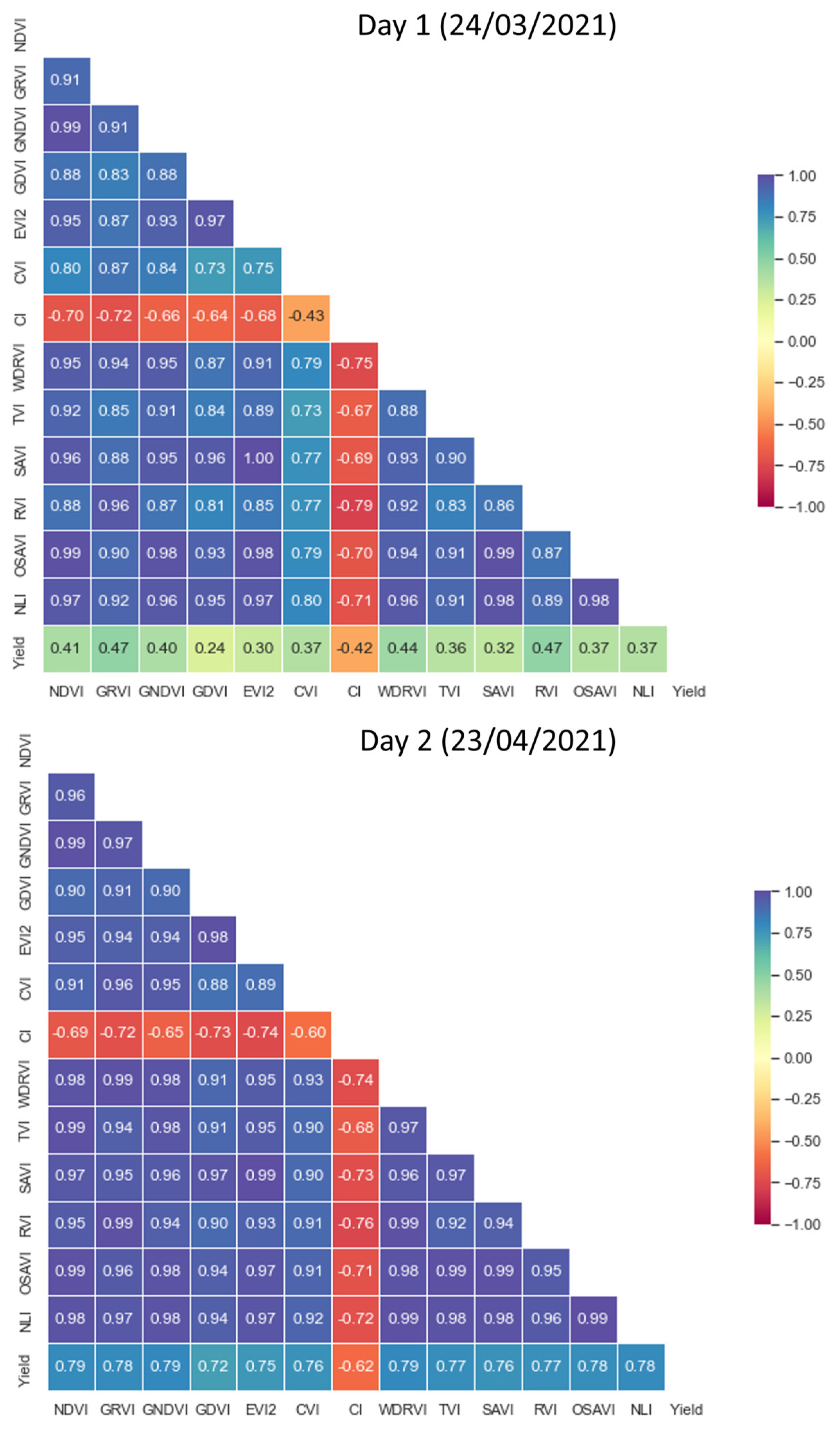
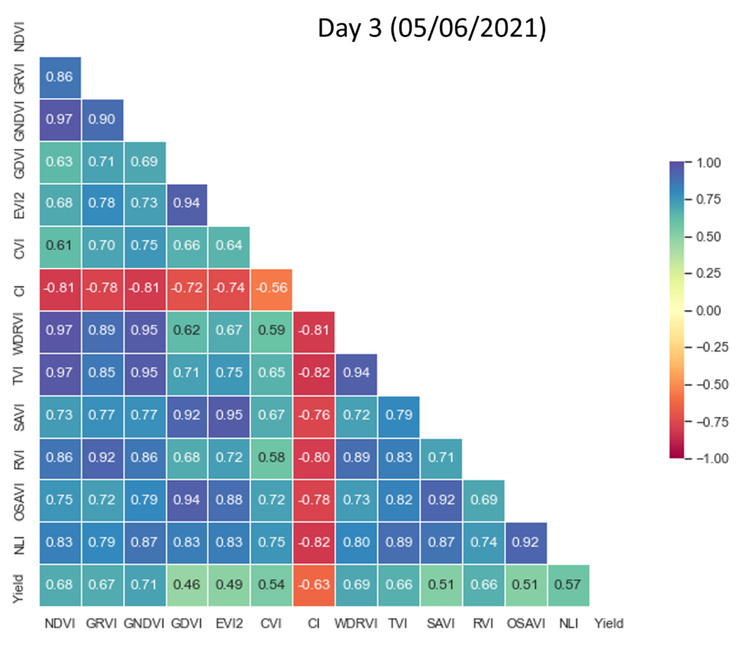
Figure 3 shows correlation matrices for the three different dates of VIs derived from S2 and yield. A high degree of collinearity among the different VIs was observed on the three dates, with Day 2 (GS39-49) showing the strongest correlation between indices with r values above 0.9. In addition to the negative correlation, when compared to the other VI results, the CI index obtained lower r values, ranging from −0.59 to −0.76 (Figure 3, Day 2). Correlations between the VIs of Day 1 (GS30) were slightly lower but remained above 0.8. Furthermore, the correlation between different VIs for Day 3 is not homogeneous (as indicated by the broader color palette of the matrix), and r values varied from 0.97 to 0.58. Given the high degree of collinearity observed among the VIs, some measures were taken to address this issue during the implementation of the different algorithms. One such measure employed was the Lasso correction of the MLR method.
In terms of the relationship between the different VIs and yield, the highest values were measured for Day 2 (GS39-49). Except for the negative correlation of CI (−0.65), the values ranged from 0.81 for GRVI to 0.73 for GDVI. In comparison, for Day 3 (GS69-75), the correlations ranged from 0.72 for GNDVI to 0.54 for GDVI. Although the increase in correlation is not significant (−0.66 compared to −0.65), CI was the only VI that increased the correlation. The lowest correlations were found with the VIs of Day 1 (Figure 3), with values ranging from 0.51 (RVI and GRVI) to 0.26 for GDVI. The correlation of CI was inverse (−0.45). Overall, the highest value was obtained with GRVI for all three dates, whereas GDVI exhibited the lowest values.

3.2. Exploring the Impact of Date Selection on Wheat Yield Prediction Using VIs Derived from Sentinel-2

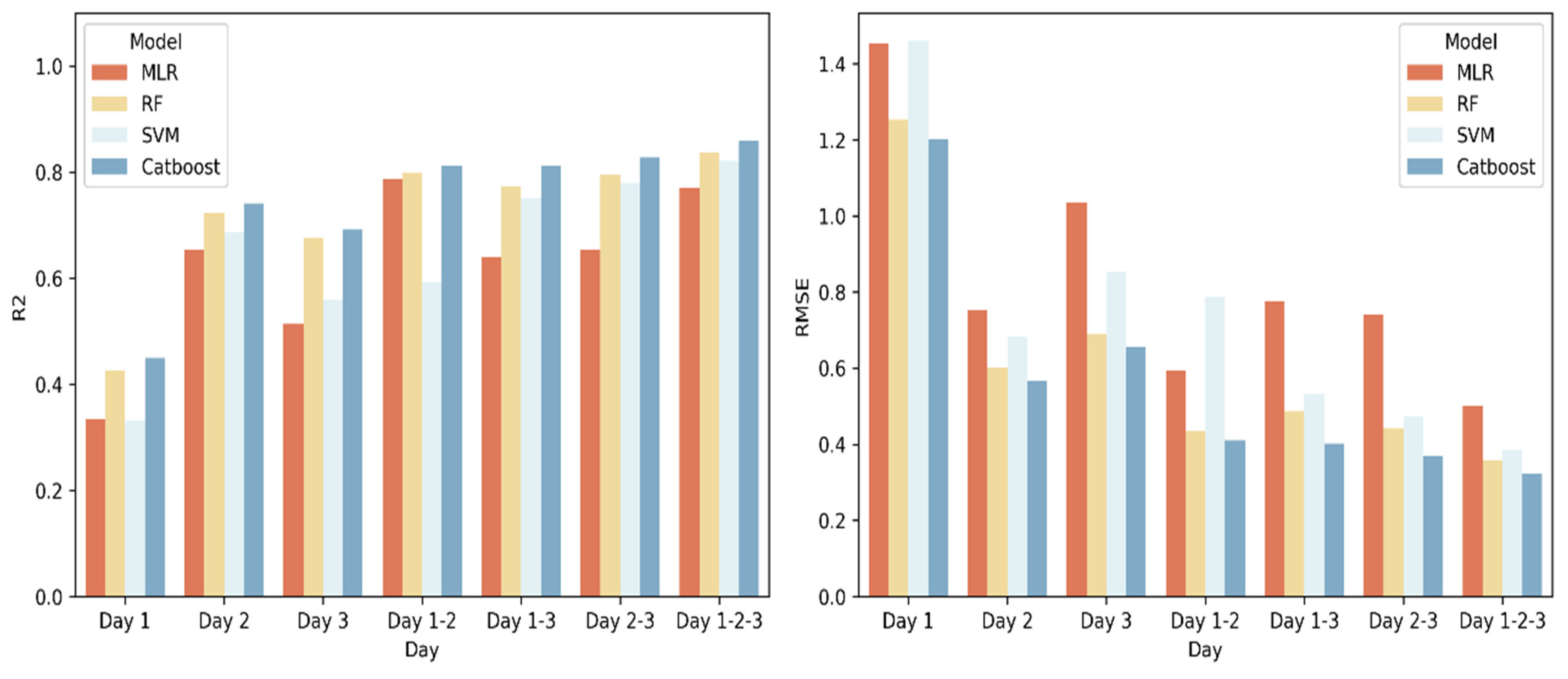
In this study, the effect of adding different VIs derived from S2 corresponding to the three dates and its combination on the prediction of wheat grain yield was investigated using four different algorithms: CatBoost, SVM, RF, and MLR. All results (RMSE and R2) (Figure 4) were obtained from the testing dataset. A consistent pattern was observed for all dates, with the best results obtained using CatBoost and the worst using MLR. When using the data from a single day, the R2 and RMSE values varied greatly depending on the date. The worst results were always obtained when using VIs from Day 1. Thus, RMSE oscillated between 1.20 for CatBoost and 1.45 for MLR while R2 ranged between 0.45 and 0.33. In contrast, the best results for a single day were obtained with Day 2 and CatBoost, reducing the RMSE to 0.56 and increasing the R2 to 0.74.
When considering the predictive ability of the model using two different dates, the performance was better than when using each day separately. The R2 of CatBoost ranged between 0.81 for the Day 1–2 dataset and 0.82 for the Day 2–3 dataset (Figure 4), while the R2 value of MLR ranged between 0.65 for the Day 1–2 dataset and 0.69 for the Day 2–3 dataset. This result suggests that the best predictions were obtained with the dates corresponding to GS39-49 and GS69-75.
Nonetheless, the results indicate that all algorithms obtained the best results when they were trained with a dataset composed of the three dates (corresponding to GS30, GS39-49, and GS69-75 phenological stages). The R2 values ranged from 0.859 for the CatBoost algorithm to 0.77 for MLR, while RMSE ranged from 0.32 for CatBoost to 0.50 for MLR.

3.3. Exploring the Impact of Date Selection on Wheat Yield Prediction Using Backscatter Information Derived from Sentinel-1

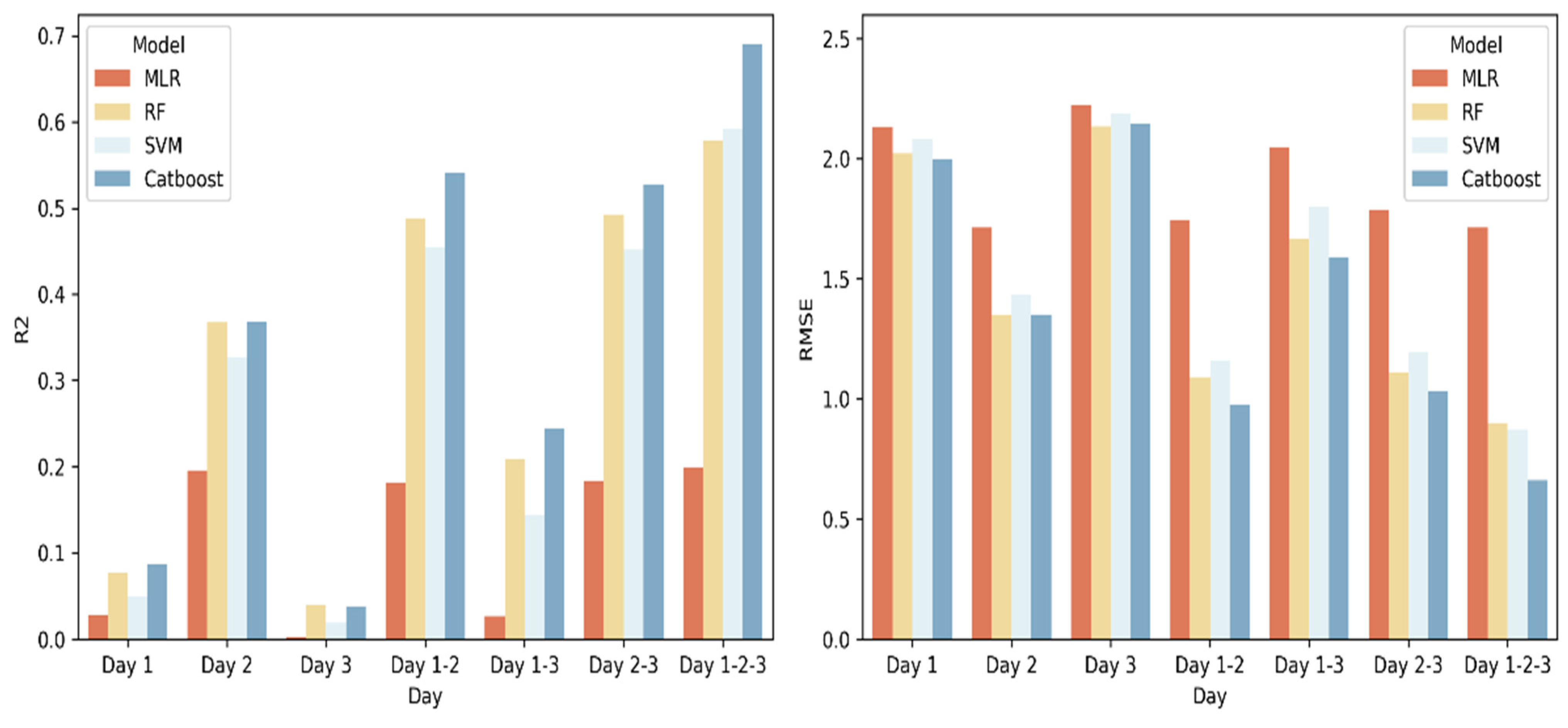
In this study, the feasibility of using backscatter information obtained from S1 at various dates to train and test machine learning models was evaluated. The results, represented in terms of R2 and RMSE, obtained during the testing process are presented in Figure 5.
The pattern observed with S2 is repeated with the S1 data, where the best results were obtained using CatBoost and the worst using MLR. In the case of employing single days, the results showed notable variations depending on the selected day. For example, the R2 value for Day 2 was 0.36, while for Day 3, it decreased to 0.08 when using CatBoost.
For the S1 data, the combination of multiple dates improved the results compared to a single date. The highest R2 values were obtained when using information from the three days (Days 1–3). Among the algorithms tested, CatBoost showed the best results with an R2 of 0.69, while the lowest R2 value of 0.20 was obtained with the MLR model (Figure 5). The RF and SVM models showed similar results, with the latter showing a slightly better performance.
It is noteworthy that combining data from multiple dates did not always result in better performance compared to using data from a single date. For example, the RMSE for Day 2 was 1.34, while the combination of Days 1–3 was 1.59 with the CatBoost algorithm.
Additionally, the greatest differences in the RMSE and R2 were observed between the algorithms that can analyze non-linear relationships (RF, SVM, and CatBoost) and the one that only analyzes linear relationships (MLR) when compared to the information of S2. In all cases, the non-linear algorithms showed better results (Figure 5).

3.4. Comparison of Machine Learning Algorithms for Estimating Wheat Yield Using Multisource Data

The results presented in the previous section indicate that the best results were consistently obtained using the information from Day 1-2-3. Having determined the optimal date combination, the next objective was to determine which algorithm achieved the best results for it. For this purpose, the RMSE and rRMSE were used. To capture the variability of each algorithm more accurately, the authors trained and validated each algorithm 10 times using different partitions of three datasets (S1, S2, and S1S2), resulting in 30 RMSE and rRMSE values for each algorithm (Table 2).
Table 2 shows the statistics associated to the prediction error obtained after running each algorithm 10 times with each of the three datasets (S1, S2 and S12). CatBoost produced the lowest error with an RMSE of 0.41 t ha-1 and a mean rRMSE of 5.91%. The SD of the RMSE for CatBoost was 0.29, the lowest among the four models. CatBoost not only produced results that were closest to the actual data, but also had less variability in the results compared to the other algorithms. RF and SVM performed similarly, with an average RMSE of 0.69 and 0.62 t ha−1, respectively. The values of rRMSE were 9.78% and 8.92% (Table 2). The SD for both was nearly the same, 0.35 for RF and 0.34 for SVM. Finally, MLR produces the highest mean RMSE of 1.1 t ha−1, with a mean rRMSE of 15.25% and an SD of 0.77.
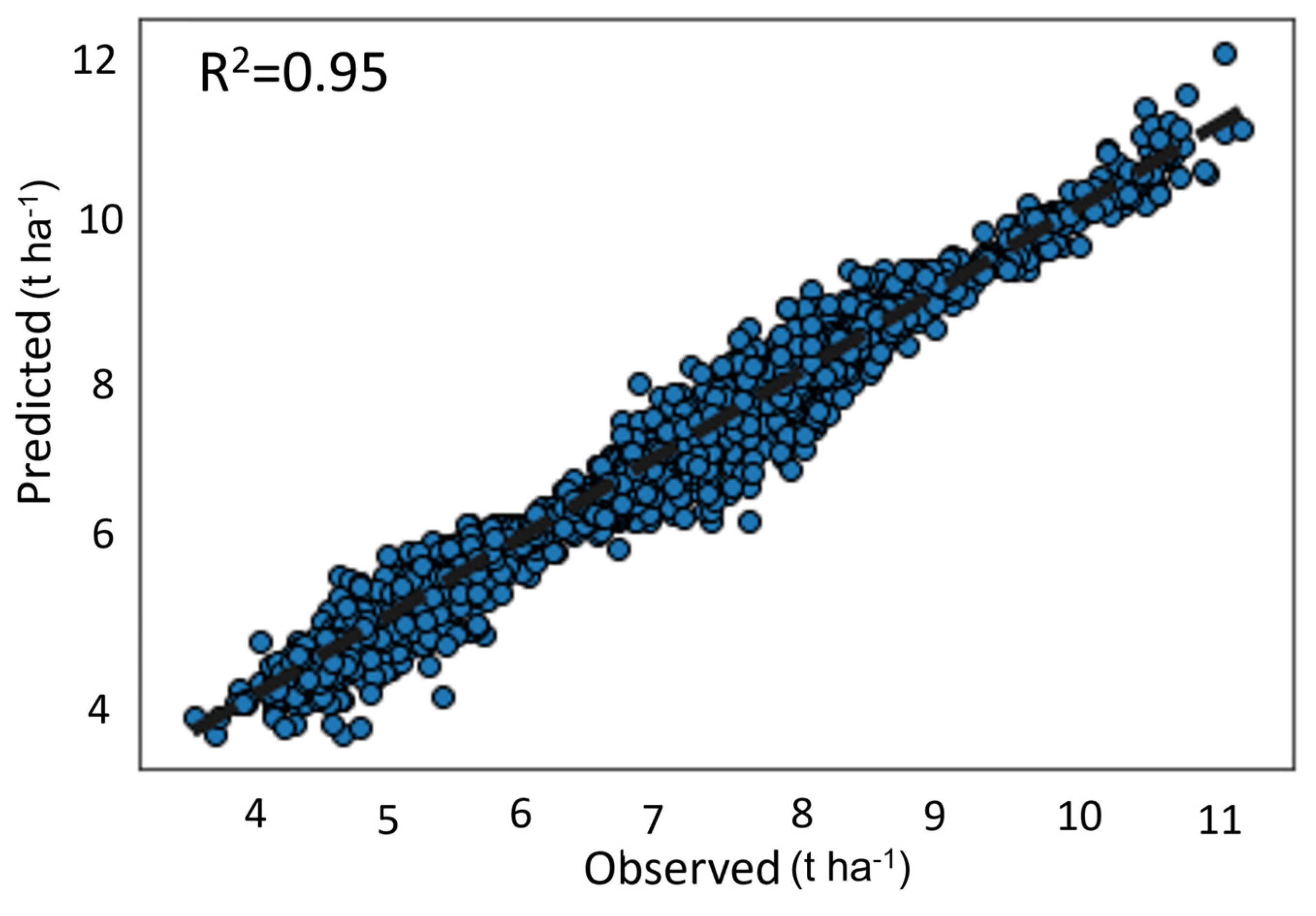
After determining that CatBoost was the algorithm with the lowest RMSE and rRMSE among the four evaluated algorithms, the subsequent step involved evaluating the performance of CatBoost with each dataset (S1, S2, and S1S2). To this end, CatBoost was trained and tested with each of the three datasets 10 times with different partitions of data to train and test. The results presented in Figure 6 show that the RMSE varied depending on the dataset used for yield estimation. The use of the S1S2 dataset produced the lowest error, with a mean RMSE of 0.24 t ha−1, which is an rRMSE of 3.46%. The RMSE values ranged between 0.22 and 0.26 t ha−1. The mean RMSE obtained with S2 was 0.34 t ha−1 and the rRMSE was 4.86%. RMSE values ranged from 0.30 to 0.37 t ha−1 (Figure 6). Finally, the highest RMSE values were obtained when using only S1 data, with a mean RMSE of 0.79 t ha−1 and values ranging from 0.55 to 0.83 t ha−1. The rRMSE for the S1 dataset was 11.34%. Therefore, the use of combined S1 and S2 (S1S2) data reduced the error by 30% compared to using S2 data alone. Figure 7 presents the comparison of the predicted values versus the real values using CatBoost with S1S2. The R2 value was 0.95.

3.5. Contribution of the Variables to the Defintive Algorithm

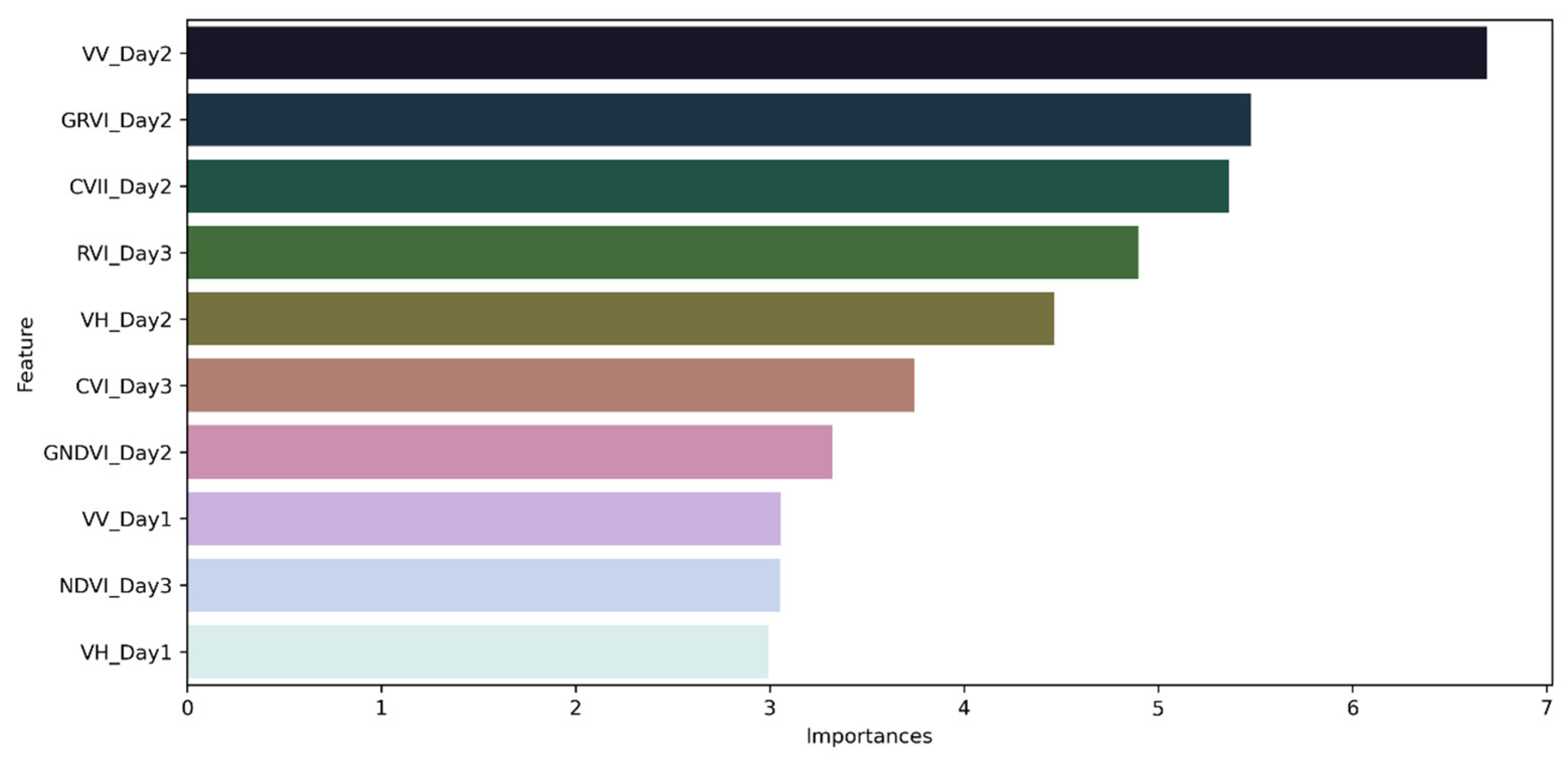
Figure 8 shows the 10 variables that made the greatest contribution to the CatBoost model, explaining 43.05% of the total variability. Of the 45 variables used (13 VIs and two backscatter variables for each day), the VV polarization variable (VV_Day2) derived from S1 and corresponding to April 20 (Day 2; GS39-49) contributed most to the model, with 6.69% of the explained variability. The second highest contributor was the GRVI_Day2 variable, which explained 5.47% of the variability. This variable, derived from S2, corresponds to April 23. The VH_Day1 variable, as shown in Figure 8, explained 2.99% of the total variability.
The analysis of the variables derived from S2 revealed a predominance of those obtained on Day 2 (April 20, GS39-49). However, there was also a representation of those from Day 3 (June 5, GS69-75), such as RVI. It is notable that the CVI variable is the only VI represented on two different days. With respect to the variables derived from S1, those corresponding to Day 2 explained more variability. However, in contrast to those derived from S2, in the case of S1 Day 1 (GS30) variables explained more variability than Day 3 (GS69-75) variables. Although the acquisition date is deemed more pertinent, polarization holds significance due to the greater explanatory power of the VV variables compared to the VH variables.

3.6. The Ability of CatBoost to Predict Yield of Entire Plots Using Data from Other Plots

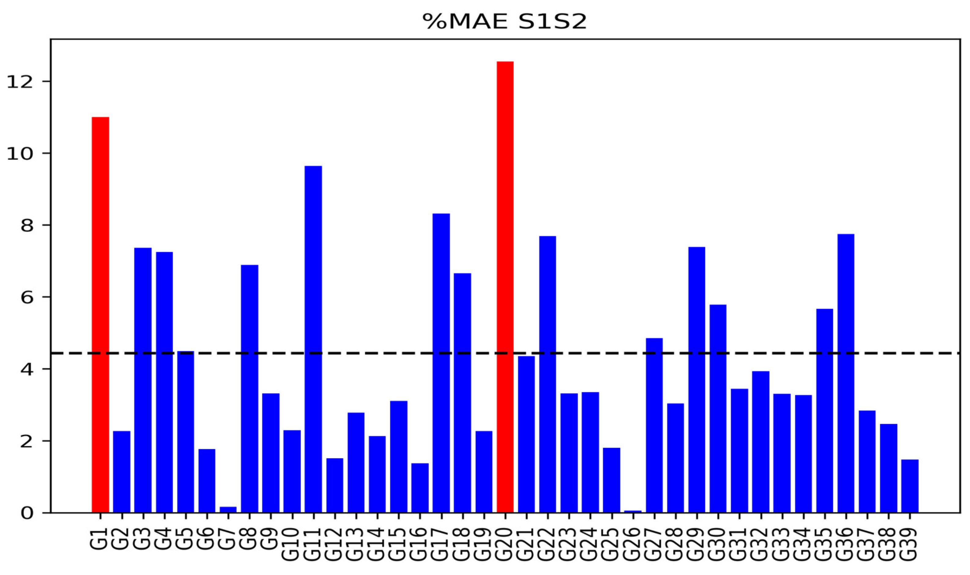
In this section, the study aimed to evaluate the ability of CatBoost to predict the yield of an entire plot using information from other plots. Figure 9 shows that the mean %MAE was 4.38, which is below the acceptable error of 10%. However, plots G1 and G20 exceeded the 10% MAE threshold (Figure 9). To visually represent the difference between the actual and predicted yield values, G15 was selected.
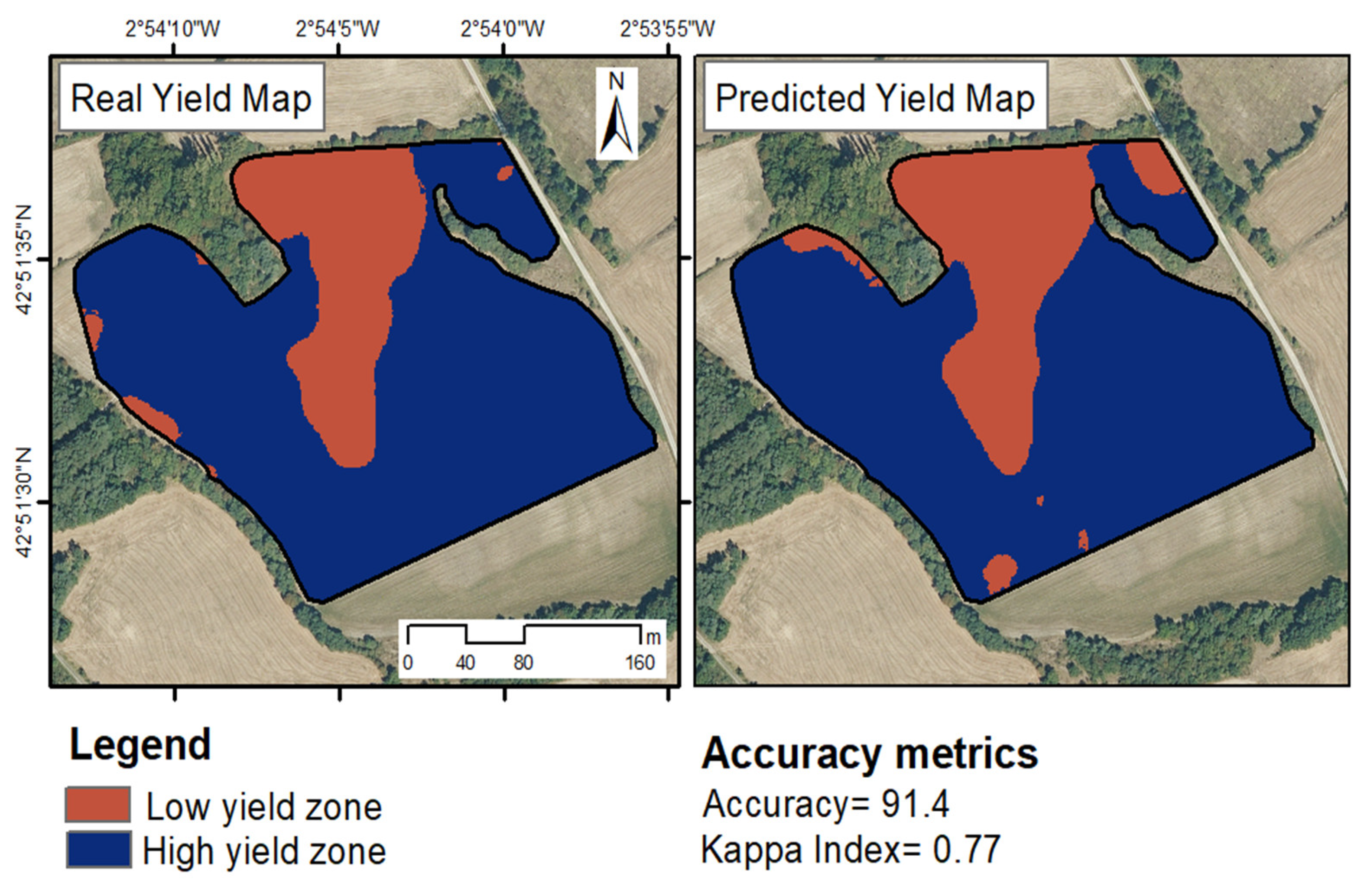
Each dataset (measured and estimated yield data) was classified into two different classes using the ISODATA algorithm, which automatically set the optimal threshold for classification. The threshold for the measured data was set at 5.17 t ha−1, while for the estimated data, it was set at 5.23 t ha−1. To compare the agreement between the two classified maps, the accuracy and KI metrics were used. The accuracy was found to be 91.4%, while the KI was 0.77 (Figure 10). The accuracy and KI metrics show that the two classified maps are similar, indicating that the estimated map has retained the spatial variability of the original data. For G15 plot, the model predicted an average yield error of 0.190 t ha−1, which is less than the maximum established error.

4. Discussion

4.1. Inclusion of Sentinel-1 and Sentinel-2 in the Yield Estimation Model

In this study, an analysis was conducted to examine the impact of incorporating multiple variables derived from S2 bands (VIs) and S1 backscatter information with VV and VH polarization obtained from various dates on yield prediction. The results revealed a consistent pattern in which the most favorable outcomes were consistently achieved when utilizing data from all three specified dates that corresponded to the GS30, GS39-49, and GS69-75 phenological stages.
In this study, the results obtained from VIs were consistent with those reported in prior research by Hunt et al. [29], since the inclusion of data from various dates improved model accuracy. In their study, the RF model was tested using VIs obtained from December to July, and the best results were obtained when using the VIs from all months together. According to the literature, the best grain yield estimation results are typically obtained after the end of the stem elongation phase (>GS39) [91,92], with the strongest relationship occurring during the anthesis or milky grain phase [93]. However, the analysis of VI information using data from only one day revealed that the optimal results were obtained using data corresponding to Day 2 (GS39-49) (Figure 3), which corresponds to the period from the end of stem elongation until the first awns’ visible growth stage (24 April). This correlation was slightly higher than that achieved with data from Day 3 when wheat is between complete anthesis and medium milk phase GS69-75 (5 June). Despite the moderate to high collinearity among the VIs on the three dates (Figure 3), the results presented in Section 3.1 suggest that it is beneficial to use all the indices and multiple dates to obtain the best results. Furthermore, it is evident that the use of any model is superior to the use of only one index when predicting wheat yield.
Hunt et al. [29] found that the greatest improvement in the model occurred between December and April for wheat fields in the UK, with the improvement thereafter being less significant. In this study, the mean correlation coefficient between VI and yield on Day 1 (GS30) was 0.36, while on Day 2 (GS39-49), it increased to 0.78 (Figure 3). Additionally, other authors such as Segarra et al. [35] have reported that the best results (R2 = 0.89) were obtained with the leaf area index (LAI) corresponding to the stem elongation/heading stage, and the results with VIs were similar (R2 = 0.88). This is not surprising since LAI and some VIs are related [69]. Correlation between grain yield and VIs and LAI at this phase is logical since the phases encompassing stem elongation to ear growth phases are crucial in the vegetative growth of wheat [94] and greatly determine the final grain yield. The models demonstrated a high degree of efficiency in their ability to estimate yield at the end of April (GS39-49). Although it may be late to make decisions that improve yield in rainfed conditions, it could be useful for the planning of future fertilizer decisions within the framework of precision fertilization.
Analysis of the S1 backscatter information revealed that the best results were obtained using data from Day 2, corresponding to 20 April. However, in contrast to the results obtained with S2, the data from Day 1 explained more variability than Day 3 data (as seen in Figure 5). Previous research has reported a positive correlation between wheat yield and the backscattering coefficient from S1 [95]. This correlation can be attributed to the fact that backscattering is sensitive to changes in crop growth, biomass, and soil water content, all crucial factors in determining wheat yield [96]. In the early growth stages, stronger correlations were reported when backscatter information was used [96]. During these stages, the crop is more sensitive to variations in water and nutrient availability [97], and variations in backscattering can indicate crop health and potential yield. Furthermore, the correlation between the backscattering coefficient and wheat yield is more robust in areas where wheat is grown in monoculture. This is because the crop canopy in monoculture is more homogenous, and the backscattering signal can be more directly linked to crop growth and yield.
For the three S1 images, the VV polarization was found to contribute more to the model, in contrast to the results reported by Mandal et al. [98] who found higher correlations with VH polarization. The reason behind this is that VH polarization is more sensitive to changes in surface roughness, which is an indicator of crop growth, whereas VV polarization captures better changes in soil water content and soil moisture [99]. This seems to indicate that soil water content in the crop early stages affects the final yield in a relevant way. It is noteworthy that the correlation between backscattering and wheat yield is not simple, thus it is understandable that a higher R2 value was obtained when using S2 data than S1 (Figure 4 and Figure 5).

4.2. Reasons Why the Combination of Information from Sentienel-1 and Sentinel-2 Enhances the Yield Estimation Model

Previous studies, such as those published by Mercier et al. [100], have utilized data from S1 to predict the phenological stage of wheat. Other investigations have employed the combined information from S1 and S2 for the same purpose [101]. For example, Chaucha et al. [102] used the combined data from both satellites to determine wheat lodging in specific plots. Thus, there are previous studies in which the combined information from S1 and S2 has been utilized to estimate properties that can impact wheat yield or monitor crop development. However, to date, no studies have been identified in the literature that employ the combined information from both satellites to directly estimate wheat yield.
The findings of this study indicate that the utilization of data from both satellites improves the RMSE when compared to results obtained using only data from S2 (Figure 6). Establishing a relationship between wheat grain yield and S1 backscatter is not straightforward as the correlation is not linear, as shown by the performance of MLR (Figure 5). The backscatter is associated with crop canopy and soil roughness, which is related to crop development, LAI, biomass, and grain yield [103]. On the other hand, VIs derived from S2 data are relatively simple to calculate, are not computationally intensive, and are usually related to the biophysical properties of crops, such as greenness and health [104]. However, multicollinearity is a problem when using multiple VIs (Figure 3), as it reduces model accuracy [105]. The analysis of variable contribution showed that, among the top ten most representative variables, variables from both sources of information were present (Figure 8). Despite the unexpected nature of this finding, the variable that demonstrated the greatest contribution in the model was VV_Day2. This is particularly surprising because VH polarization is usually more sensitive to crop changes than VV [98]. By using data from both S1 and S2 satellite sources together, a more comprehensive understanding of the crop can be obtained, which can lead to more accurate wheat yield predictions. This study demonstrates the potential of using combined S1 and S2 data for crop monitoring and yield prediction and highlights the importance of considering multiple data sources for more accurate crop assessment.

4.3. Algorithm Analysis

The results obtained through the utilization of RF, SVM, and CatBoost algorithms surpassed those obtained through the utilization of MLR in all scenarios. The greatest error measured with RMSE was observed when the model was trained with S1 data, as depicted in Figure 5. The reason for this is that the connection between backscatter and yield is not linear, and MLR is not able to handle non-linear relationships. Although the relationship between VIs and wheat yield is primarily linear, it possesses enough non-linearity for other algorithms to yield superior results [106]. The capacity to handle non-linear relationships is a key advantage of some algorithms (SVM, RF, CatBoost), as it enables the analysis of complex multivariate relationships between different types of data, which is not feasible with MLR. The results obtained through the utilization of RF and SVM are comparable, with those obtained using the SVM model being slightly superior, which is in contrast to those reported by other authors [35,107] in the field of wheat yield prediction. Although RF generally outperforms SVM, in some areas of PA such as disease detection, SVM has performed better than RF [108]. However, in this study, the best results were achieved using the CatBoost algorithm, which is a member of the boosting algorithm family. The algorithms belonging to this family have produced inconsistent outcomes within the domain of PA. For example, Bebie et al. [25] reported the worst results when the boosting regression (BR) algorithm was used, while Heremans et al. [108] obtained the best outputs with the same algorithms. CatBoost, like Xtreme Gradient Boosting (XGBoost), is a gradient boosting algorithm that belongs to the next generation of boosting algorithms, and XGBoost has been used successfully in PA to predict monthly NDVI evolution [109]. However, the use of this group of algorithms is not as prevalent in PA as RF or SVM. As an example, the Scopus database revealed a limited number of articles, only seven, that employ CatBoost within any field of PA. In contrast, it is widely utilized in other areas such as industries, finance, healthcare, and online advertising.
Although in this case it has not been used because all the variables are quantitative, one of the main advantages of CatBoost over other algorithms is its ability to handle categorical variables because it can automatically deal with them without any additional pre-processing, such as ‘one hot encoding’ reducing considerably matrix dimensions. Moreover, CatBoost is specifically engineered to handle large datasets, as it facilitates training on graphics processing units (GPUs), thereby significantly decreasing computation time. In terms of performance, CatBoost has been shown to have high performance and generalization ability, outperforming other algorithms such as RF and the generalized regression neural network (GRNN) algorithm [110]. Additionally, CatBoost has a built-in mechanism for handling overfitting, which can be a problem with other algorithms like deep neural networks (DNNs) [111] and missing values. Finally, CatBoost also has a built-in feature importance mechanism that allows users to understand the importance of each feature in the dataset.

4.4. CatBoost Algorithm as a Tool for Processing Heterogeneous Data in Precision Agriculture

Use of the CatBoost algorithm in PA can provide significant advantages in terms of scaling up results. This algorithm is based on gradient boosting and is specifically designed to handle both numerical and categorical variables. This characteristic makes it suitable for PA, where a large amount of heterogeneous data are generated.
Compared to traditional machine learning algorithms such as RF, CatBoost has demonstrated improved performance in terms of accuracy and speed. The algorithm utilizes decision trees as weak learners and combines them in an iterative manner to make a strong prediction model. This results in a model that can generalize well to new data and is able to handle large amounts of data more efficiently than traditional algorithms.
In PA, the use of remote sensing data is increasingly common. This technology allows the acquisition of information on the physical, chemical, and biological characteristics of crops. Integration of the CatBoost algorithm with remote sensing data can provide valuable insights into crop growth. Another advantage of CatBoost is its ability to operate effectively even in the presence of missing records in a database. This is a common challenge faced when utilizing information from multiple sensors, as failures of individual sensors can occur at any point in time. The application of techniques to address such situations is not ideal, as it involves the addition of estimated information, which does not enhance the model. Furthermore, CatBoost data does not require scaling, leading to reduced time and effort in data preprocessing.

4.5. Potential of S1 Backscatter and VIs for Precise Yield Mapping in Rainfed Areas Using the CatBoost Algorithm

VIs have been widely utilized in PA for various purposes such as yield estimation, SSMZ delimitation, and water stress estimation. For its part, S1 backscatter information has been used for crop classification or for measuring land transformation changes. However, its use for yield estimation is not common. As previously mentioned, its relationship with growth is not direct, but it has been associated with key factors such as soil moisture, roughness or crop height. Therefore, it is imperative to conduct new studies to understand the underlying relationship between wheat yield and the S1 backscatter signal.
This study represents a preliminary step towards the goal of modulating fertilizer application according to crop needs. The underlying theoretical basis of this approach is that in rainfed areas, the fertilizer needs of the crop are generally associated to the potential yield. The high resolution of this study allowed for the estimation of precise yield maps. In this sense and according to Figure 9, the average %MAE was 4.38%, equivalent to an error of 0.31 t ha−1. This level of precision would enable farmers to adjust fertilizer rates at the plot level with an acceptable margin of error. Figure 10 takes this approach one step further by comparing the yield maps generated from the yield monitor data with those generated using the proposed methodology. The classification of pixels was found to be consistent between the two maps in 91.4% of cases, suggesting that this approach captures intra-plot yield spatial variability. Therefore, this would enable farmers who do not have a yield monitor installed on their harvesters but have a variable rate fertilizer applicator to create and employ intra-plot prescription maps based on estimated yield maps. In addition, thanks to the auxiliary information source used (VI and backscatter derived from satellites), this methodology can be scalable and applicable to larger areas. The results, however, were obtained using satellite images acquired between Day 1 (GS30) and Day 3 (GS69-75), with the latter date being too late to increase yield by fertilizing. Considering this, the authors believe that future works should be directed at studying the combined capability of CatBoost with remote sensing data at early phenological stages of the crop to vary the fertilization strategy during the growing cycle.
Finally, it is worth noting that the results presented in this study are promising, but only correspond to one year. Thus, future works should encompass data from several years to verify that the results remain consistent across all campaigns. Furthermore, it would be interesting in future studies to incorporate high resolution climate and soil information in order to better understand the reasons behind yield spatial variability.

5. Conclusions

The models developed to estimate yield using information from S1 and S2 satellites showed better results than the correlation analysis. Among the evaluated models, CatBoost, which is still relatively underutilized in agriculture, provided the best results. Furthermore, using all available images that correspond to the GS30, GS39-49 and GS69-75 wheat phenological phases improved the performance of the models. Additionally, combining images from S1 and S2 substantially improved predictions, providing a level of precision sufficient to consider yield maps for fertilizer adjustment. This is an important aspect because most farmers in the area do not have yield monitors.
Despite its potential, the methodology proposed in this article has some limitations. Operationally, the biggest challenge lies in the clouds that impact the usability of the S2 images. While, theoretically, S2 provides an image every five days, in reality only three images were obtained throughout the whole crop growing cycle which were free of clouds and hence suitable for analysis. Moreover, to effectively train the algorithm, it is imperative to have access to high resolution yield data, such as that provided by yield monitors, although the use of such equipment is not yet widespread.
Combining the backscatter information of S1 with that of S2 resulted in improved outcomes of only using data from S2. However, further research is necessary to gain a better understanding of the relationship between backscattering and crop yield. In addition, this study focused solely on VIs and backscattering as they provide information on crop status. Future research could benefit from incorporating high resolution meteorological and edaphic variables, such as temperature, precipitation, and soil moisture, to better comprehend the factors influencing crop yield.

Author Contributions

A.U. worked in the following: Conceptualization, Methodology, Software, Data Processing, Formal Analysis, Original Draft Preparation, Visualization, Investigation, Interpretation. A.C. worked in the following: Methodology, Data Acquisition, Results Analysis, Resources. A.A. worked in the following: Conceptualization, Methodology, Writing, Reviewing and Editing, Supervision of Parameter Computing, Funding Acquisition, Project Administration. All authors have read and agreed to the published version of the manuscript.

Funding

This work was funded by the AgritechZeha project of the Basque Government, Department of Economic Development, Sustainability and Environment. It also was partially elaborated in the context of the CLIMALERT project SOE3/P4/F0862 UNION EUROPE. So, we want to express our gratitude to Interreg Sudoe Programme which a is part of the European territorial cooperation objective known as Interreg (financed by one of the European structural funds: the European Regional Development Fund (ERDF)).

Data Availability Statement

Data are available in a publicly accessible repository that does not issue DOIs. The raw satellite information data can be found in https://scihub.copernicus.eu/dhus/#/home, accessed on 30 January 2023.

Acknowledgments

The authors would like to thank Javier Alava, a farmer in the GARLAN cooperative, for providing the possibility to carry out the research in his plots and giving us high resolution yield information.

Conflicts of Interest

The authors declare no conflict of interest. The funders had no role in the design of the study, in the collection, analyses, or interpretation of data, in the writing of the manuscript, or in the decision to publish the results.

References

  1. Giller, K.E.; Delaune, T.; Silva, J.V.; Descheemaeker, K.; van de Ven, G.; Schut, A.G.; van Wijk, M.; Hammond, J.; Hochman, Z.; Taulya, G.; et al. The future of farming: Who will produce our food? Food Secur. 2021, 13, 1073–1099. [Google Scholar] [CrossRef]
  2. Pingali, P.L. Green Revolution: Impacts, limits, and the path ahead. Proc. Natl. Acad. Sci. USA 2012, 109, 12302–12308. [Google Scholar] [CrossRef] [Green Version]
  3. Wik, M.; Pingali, P.; Broca, S. Global Agricultural Performance: Past Trends and Future Prospects; World Bank: Washington, DC, USA, 2008. [Google Scholar]
  4. Hazell, P. Handbook of Agricultural Economics; Pingali, P., Evenson, R., Eds.; Elsevier: Amsterdam, The Netherlands, 2010; pp. 3469–3530. [Google Scholar]
  5. Randall, G.; Goss, M. Nitrate Losses to SurfaceWater through Subsurface, Tile Drainage. In Nitrogen in the Environment: Sources, Problems, and Management; Elsevier: Amsterdam, The Netherlands, 2008. [Google Scholar]
  6. Snyder, C.; Bruulsema, T.; Jensen, T.; Fixen, P. Review of greenhouse gas emissions from crop production systems and fertilizer management effects. Agric. Ecosyst. Environ. 2009, 133, 247–266. [Google Scholar] [CrossRef]
  7. Ziliani, M.G.; Altaf, M.U.; Aragon, B.; Houborg, R.; Franz, T.E.; Lu, Y.; Sheffield, J.; Hoteit, I.; McCabe, M.F. Early season prediction of within-field crop yield variability by assimilating CubeSat data into a crop model. Agric. For. Meteorol. 2022, 313, 108736. [Google Scholar] [CrossRef]
  8. Zambon, I.; Cecchini, M.; Egidi, G.; Saporito, M.G.; Colantoni, A. Revolution 4.0: Industry vs. Agriculture in a Future Development for SMEs. Processes 2019, 7, 36. [Google Scholar] [CrossRef] [Green Version]
  9. Mumtaz, R.; Baig, S.; Fatima, I. Analysis of meteorological variations on wheat yield and its estimation using remotely sensed data. A case study of selected districts of Punjab Province, Pakistan (2001–2014). Ital. J. Agron. 2017, 12, 897. [Google Scholar] [CrossRef]
  10. Sandonís-Pozo, L.; Llorens, J.; Escolà, A.; Arnó, J.; Pascual, M.; Martínez-Casasnovas, J.A. Satellite multispectral indices to estimate canopy parameters and within-field management zones in super-intensive almond orchards. Precis. Agric. 2022, 23, 2040–2062. [Google Scholar] [CrossRef]
  11. Uribeetxebarria, A.; Arnó, J.; Escolà, A.; Martínez-Casasnovas, J.A. Apparent electrical conductivity and multivariate analysis of soil properties to assess soil constraints in orchards affected by previous parcelling. Geoderma 2018, 319, 185–193. [Google Scholar] [CrossRef] [Green Version]
  12. Del-Moral-Martínez, I.; Rosell-Polo, J.R.; Company, J.; Sanz, R.; Escolà, A.; Masip, J.; Martínez-Casasnovas, J.A.; Arnó, J. Mapping Vineyard Leaf Area Using Mobile Terrestrial Laser Scanners: Should Rows be Scanned On-the-Go or Discontinuously Sampled? Sensors 2016, 16, 119. [Google Scholar] [CrossRef] [Green Version]
  13. Daberkow, S.G.; McBride, W.D. Farm and Operator Characteristics Affecting the Awareness and Adoption of Precision Agriculture Technologies in the US. Precis. Agric. 2003, 4, 163–177. [Google Scholar] [CrossRef]
  14. Chen, W.; Bell, R.W.; Brennan, R.F.; Bowden, J.W.; Dobermann, A.; Rengel, Z.; Porter, W. Key crop nutrient management issues in the Western Australia grains industry: A review. Soil Res. 2009, 47, 1–18. [Google Scholar] [CrossRef]
  15. Barnes, A.; Soto, I.; Eory, V.; Beck, B.; Balafoutis, A.; Sánchez, B.; Vangeyte, J.; Fountas, S.; van der Wal, T.; Gómez-Barbero, M. Exploring the adoption of precision agricultural technologies: A cross regional study of EU farmers. Land Use Policy 2019, 80, 163–174. [Google Scholar] [CrossRef]
  16. Ingram, J. Agronomist–farmer knowledge encounters: An analysis of knowledge exchange in the context of best management practices in England. Agric. Hum. Values 2008, 25, 405–418. [Google Scholar] [CrossRef]
  17. Segarra, J.; Buchaillot, M.L.; Araus, J.L.; Kefauver, S.C. Remote Sensing for Precision Agriculture: Sentinel-2 Improved Features and Applications. Agronomy 2020, 10, 641. [Google Scholar] [CrossRef]
  18. Ghosh, P.; Mandal, D.; Bhattacharya, A.; Nanda, M.K.; Bera, S. Assessing crop monitoring potential of sentinel-2 in a spatio-temporal scale. ISPRS Int. Arch. Photogramm. Remote Sens. Spat. Inf. Sci. 2018, XLII-5, 227–231. [Google Scholar] [CrossRef] [Green Version]
  19. Yi, Z.; Jia, L.; Chen, Q. Crop Classification Using Multi-Temporal Sentinel-2 Data in the Shiyang River Basin of China. Remote Sens. 2020, 12, 4052. [Google Scholar] [CrossRef]
  20. Sadeghi, M.; Babaeian, E.; Tuller, M.; Jones, S.B. The optical trapezoid model: A novel approach to remote sensing of soil moisture applied to Sentinel-2 and Landsat-8 observations. Remote Sens. Environ. 2017, 198, 52–68. [Google Scholar] [CrossRef] [Green Version]
  21. Vallentin, C.; Harfenmeister, K.; Itzerott, S.; Kleinschmit, B.; Conrad, C.; Spengler, D. Suitability of satellite remote sensing data for yield estimation in northeast Germany. Precis. Agric. 2022, 23, 52–82. [Google Scholar] [CrossRef]
  22. Barnett, T.; Thompson, D. Large-area relation of landsat MSS and NOAA-6 AVHRR spectral data to wheat yields. Remote Sens. Environ. 1983, 4, 277–290. [Google Scholar] [CrossRef]
  23. Maselli, F.; Conese, C.; Petkov, L.; Gilabert, M.-A. Use of NOAA-AVHRR NDVI data for environmental monitoring and crop forecasting in the Sahel. Preliminary results. Int. J. Remote Sens. 1992, 13, 2743–2749. [Google Scholar] [CrossRef]
  24. Hamar, D.; Ferencz, C.; Lichtenberger, J.; Tarcsai, G.; Ferencz-Árkos, I. Yield estimation for corn and wheat in the Hungarian Great Plain using Landsat MSS data. Int. J. Remote Sens. 1996, 17, 1689–1699. [Google Scholar] [CrossRef]
  25. Bebie, M.; Cavalaris, C.; Kyparissis, A. Assessing Durum Wheat Yield through Sentinel-2 Imagery: A Machine Learning Approach. Remote Sens. 2022, 14, 3880. [Google Scholar] [CrossRef]
  26. Shen, J.; Evans, F.H. The Potential of Landsat NDVI Sequences to Explain Wheat Yield Variation in Fields in Western Australia. Remote Sens. 2021, 13, 2202. [Google Scholar] [CrossRef]
  27. Trombetta, A.; Iacobellis, V.; Tarantino, E.; Gentile, F. Calibration of the AquaCrop model for winter wheat using MODIS LAI images. Agric. Water Manag. 2016, 164, 304–316. [Google Scholar] [CrossRef]
  28. Boissard, P.; Guérif, M.; Pointel, J.-G.; Guinot, J.-P. Application of SPOT data to wheat yield estimation. Adv. Space Res. 1989, 9, 143–154. [Google Scholar] [CrossRef]
  29. Hunt, M.L.; Blackburn, G.A.; Carrasco, L.; Redhead, J.W.; Rowland, C.S. High resolution wheat yield mapping using Sentinel-2. Remote Sens. Environ. 2019, 233, 111410. [Google Scholar] [CrossRef]
  30. Li, H.; Chen, Z.; Liu, G.; Jiang, Z.; Huang, C. Improving Winter Wheat Yield Estimation from the CERES-Wheat Model to Assimilate Leaf Area Index with Different Assimilation Methods and Spatio-Temporal Scales. Remote Sens. 2017, 9, 190. [Google Scholar] [CrossRef] [Green Version]
  31. Curnel, Y.; de Wit, A.J.W.; Duveiller, G.; Defourny, P. Potential performances of remotely sensed LAI assimilation in WOFOST model based on an OSS Experiment. Agric. For. Meteorol. 2011, 151, 1843–1855. [Google Scholar] [CrossRef]
  32. Rodriguez, J.C.; Duchemin, B.; Hadria, R.; Watts, C.; Garatuza, J.; Chehbouni, A.; Khabba, S.; Boulet, G.; Palacios, E.; Lahrouni, A. Wheat yield estimation using remote sensing and the STICS model in the semiarid Yaqui valley, Mexico. Agronomy 2004, 24, 295–304. [Google Scholar] [CrossRef] [Green Version]
  33. Vicente-Serrano, S.M.; Prats, J.M.C.; Romo, A. Early prediction of crop production using drought indices at different time-scales and remote sensing data: Application in the Ebro Valley (north-east Spain). Int. J. Remote Sens. 2006, 27, 511–518. [Google Scholar] [CrossRef]
  34. Moriondo, M.; Maselli, F.; Bindi, M. A simple model of regional wheat yield based on NDVI data. Eur. J. Agron. 2007, 26, 266–274. [Google Scholar] [CrossRef]
  35. Segarra, J.; Araus, J.L.; Kefauver, S.C. Farming and Earth Observation: Sentinel-2 data to estimate within-field wheat grain yield. Int. J. Appl. Earth Obs. Geoinf. 2022, 107, 102697. [Google Scholar] [CrossRef]
  36. Uribeetxebarria, A.; Castellón, A.; Elorza, I.; Aizpurua, A. Intra-Plot Variable N Fertilization in Winter Wheat through Machine Learning and Farmer Knowledge. Agronomy 2022, 12, 2276. [Google Scholar] [CrossRef]
  37. Meraner, A.; Ebel, P.; Zhu, X.X.; Schmitt, M. Cloud removal in Sentinel-2 imagery using a deep residual neural network and SAR-optical data fusion. ISPRS J. Photogramm. Remote Sens. 2020, 166, 333–346. [Google Scholar] [CrossRef]
  38. Phiri, D.; Simwanda, M.; Salekin, S.; Nyirenda, V.R.; Murayama, Y.; Ranagalage, M. Sentinel-2 Data for Land Cover/Use Mapping: A Review. Remote Sens. 2020, 12, 2291. [Google Scholar] [CrossRef]
  39. Torres, R.; Snoeij, P.; Geudtner, D.; Bibby, D.; Davidson, M.; Attema, E.; Potin, P.; Rommen, B.; Floury, N.; Brown, M.; et al. GMES Sentinel-1 mission. Remote Sens. Environ. 2012, 120, 9–24. [Google Scholar] [CrossRef]
  40. Ulaby, F.; Moore, R.; Fung, A. Microwave Remote Sensing Active and Passive-Volume III: From Theory to Applications; Artech House: Norwood, MA, USA, 1986. [Google Scholar]
  41. Chlingaryan, A.; Sukkarieh, S.; Whelan, B. Machine learning approaches for crop yield prediction and nitrogen status estimation in precision agriculture: A review. Comput. Electron. Agric. 2018, 151, 61–69. [Google Scholar] [CrossRef]
  42. Mishra, S.; Mishra, D.; Santra, G.H. Applications of Machine Learning Techniques in Agricultural Crop Production: A Review Paper. Indian J. Sci. Technol. 2016, 9, 1–14. [Google Scholar] [CrossRef]
  43. Shao, Y.; Campbell, J.B.; Taff, G.N.; Zheng, B. An analysis of cropland mask choice and ancillary data for annual corn yield forecasting using MODIS data. Int. J. Appl. Earth Obs. Geoinf. 2015, 38, 78–87. [Google Scholar] [CrossRef]
  44. Bhosle, K.; Musande, V. Evaluation of Deep Learning CNN Model for Land Use Land Cover Classification and Crop Identification Using Hyperspectral Remote Sensing Images. J. Indian Soc. Remote Sens. 2019, 47, 1949–1958. [Google Scholar] [CrossRef]
  45. Worrall, G.; Rangarajan, A.; Judge, J. Domain-Guided Machine Learning for Remotely Sensed In-Season Crop Growth Estimation. Remote Sens. 2021, 13, 4605. [Google Scholar] [CrossRef]
  46. Arno, J.; Martinez-Casasnovas, J.A.; Ribes-Dasi, M.; Rosell, J.R. Clustering of grape yield maps to delineate site-specific management zones. Span. J. Agric. Res. 2011, 9, 721. [Google Scholar] [CrossRef] [Green Version]
  47. Tang, X.; Liu, H.; Feng, D.; Zhang, W.; Chang, J.; Li, L.; Yang, L. Prediction of field winter wheat yield using fewer parameters at middle growth stage by linear regression and the BP neural network method. Eur. J. Agron. 2022, 141, 126621. [Google Scholar] [CrossRef]
  48. Meraj, G.; Kanga, S.; Ambadkar, A.; Kumar, P.; Singh, S.K.; Farooq, M.; Johnson, B.A.; Rai, A.; Sahu, N. Assessing the Yield of Wheat Using Satellite Remote Sensing-Based Machine Learning Algorithms and Simulation Modeling. Remote Sens. 2022, 14, 3005. [Google Scholar] [CrossRef]
  49. Wang, J.; Si, H.; Gao, Z.; Shi, L. Winter Wheat Yield Prediction Using an LSTM Model from MODIS LAI Products. Agriculture 2022, 12, 1707. [Google Scholar] [CrossRef]
  50. Srivastava, A.K.; Safaei, N.; Khaki, S.; Lopez, G.; Zeng, W.; Ewert, F.; Gaiser, T.; Rahimi, J. Winter wheat yield prediction using convolutional neural networks from environmental and phenological data. Sci. Rep. 2022, 12, 3215. [Google Scholar] [CrossRef]
  51. Cao, J.; Wang, H.; Li, J.; Tian, Q.; Niyogi, D. Improving the Forecasting of Winter Wheat Yields in Northern China with Machine Learning–Dynamical Hybrid Subseasonal-to-Seasonal Ensemble Prediction. Remote Sens. 2022, 14, 1707. [Google Scholar] [CrossRef]
  52. Freund, Y.; Schapire, R.E. Experiments with a New Boosting Algorithm. In Proceedings of the 13th International Conference on International Conference on Machine Learning, Bari, Italy, 3–6 July 1996; Morgan Kaufmann Publishers Inc.: San Francisco, CA, USA, 1996; pp. 148–156. [Google Scholar]
  53. Friedman, J.H. Greedy function approximation: A gradient boosting machine. Ann. Stat. 2001, 29, 1189–1232. [Google Scholar] [CrossRef]
  54. Chen, T.; Guestrin, C. XGBoost: A Scalable Tree Boosting System. In Proceedings of the KDD ’16: 22nd ACM SIGKDD International Conference on Knowledge Discovery and Data Mining, San Francisco, CA, USA, 13–17 August 2016; pp. 785–794. [Google Scholar] [CrossRef] [Green Version]
  55. Prokhorenkova, L.; Gusev, G.; Vorobev, A.; Dorogush, A.V.; Gulin, A. CatBoost: Unbiased Boosting with Categorical Features. arXiv 2019, arXiv:1706.09516. [Google Scholar]
  56. Cai, Y.; Guan, K.; Lobell, D.; Potgieter, A.B.; Wang, S.; Peng, J.; Xu, T.; Asseng, S.; Zhang, Y.; You, L.; et al. Integrating satellite and climate data to predict wheat yield in Australia using machine learning approaches. Agric. For. Meteorol. 2019, 274, 144–159. [Google Scholar] [CrossRef]
  57. Folberth, C.; Skalský, R.; Moltchanova, E.; Balkovič, J.; Azevedo, L.B.; Obersteiner, M.; van der Velde, M. Uncertainty in soil data can outweigh climate impact signals in global crop yield simulations. Nat. Commun. 2016, 7, 11872. [Google Scholar] [CrossRef] [Green Version]
  58. Zadoks, J.C.; Chang, T.T.; Konzak, C.F. A decimal code for the growth stages of cereals. Weed Res. 1974, 14, 415–421. [Google Scholar] [CrossRef]
  59. Beck, H.E.; Zimmermann, N.E.; McVicar, T.R.; Vergopolan, N.; Berg, A.; Wood, E.F. Data descriptor: Present and future Köppen-Geiger climate classification maps at 1-km resolution. Sci. Data 2018, 5, 180–214. [Google Scholar] [CrossRef] [Green Version]
  60. Unamunzaga, O.; Aizpurua, A.; Artetxe, A.; Besga, G.; Castroviejo, L.; Blanco, F.; de la Llera, I.; Ramos, L.; Astola, G. Asistencia Técnica Para la Caracterización Agrológica del Suelo Rústico del Municipio de Vitoria-Gasteiz. Available online: https://docplayer.es/amp/152712108-Asistencia-tecnica-para-la-caracterizacion-agrologica-del-suelo-rustico-del-municipiode-vitoria-gasteiz.html (accessed on 30 January 2021). (In Spanish).
  61. Drusch, M.; Del Bello, U.; Carlier, S.; Colin, O.; Fernandez, V.; Gascon, F.; Hoersch, B.; Isola, C.; Laberinti, P.; Martimort, P.; et al. Sentinel-2: ESA’s Optical High-Resolution Mission for GMES Operational Services. Remote Sens. Environ. 2012, 120, 25–36. [Google Scholar] [CrossRef]
  62. Rouse, J.W., Jr.; Haas, R.H.; Deering, D.W.; Schell, J.A.; Harlan, J.C. Monitoring the Vernal Advancement and Retrogradation (GreenWave Effect) of Natural Vegetation; NASA/GSFC Type III Final Report 5; NASA: Greenbelt, MD, USA, 1974; p. 371.
  63. Gitelson, A.A.; Kaufman, Y.J.; Stark, R.; Rundquist, D. Novel algorithms for remote estimation of vegetation fraction. Remote Sens. Environ. 2002, 80, 76–87. [Google Scholar] [CrossRef] [Green Version]
  64. Buschmann, C.; Nagel, M. In vivo spectroscopy and internal optics of leaves as basis for remote sensing of vegetation. In-ternational Journal of Remote Sensing. Int. J. Remote Sens. 1993, 14, 711–722. [Google Scholar] [CrossRef]
  65. Tucker, C.; Elgin, J.; McMurtrey, J.; Fan, C. Monitoring corn and soybean crop development with hand-held radiometer spectral data. Remote Sens. Environ. 1979, 8, 237–248. [Google Scholar] [CrossRef]
  66. Miura, T.; Yoshioka, H.; Fujiwara, K.; Yamamoto, H. Inter-Comparison of ASTER and MODIS Surface Reflectance and Vegetation Index Products for Synergistic Applications to Natural Resource Monitoring. Sensors 2008, 8, 2480–2499. [Google Scholar] [CrossRef] [Green Version]
  67. Vincini, M.; Frazzi, E.; D’Alessio, P. A broad-band leaf chlorophyll vegetation index at the canopy scale. Precis. Agric. 2008, 9, 303–319. [Google Scholar] [CrossRef]
  68. Escadafal, R. Remote sensing of soil color: Principles and applications. Remote Sens. Rev. 1993, 7, 261–279. [Google Scholar] [CrossRef]
  69. Gitelson, A.A. Wide Dynamic Range Vegetation Index for Remote Quantification of Biophysical Characteristics of Vegetation. J. Plant Physiol. 2004, 161, 165–173. [Google Scholar] [CrossRef] [Green Version]
  70. Bannari, A.; Morin, D.; Bonn, F.; Huete, A.R. A review of vegetation indices. Remote Sens. Rev. 1995, 13, 95–120. [Google Scholar] [CrossRef]
  71. Huete, A.R. A soil-adjusted vegetation index (SAVI). Remote Sens. Environ. 1988, 25, 295–309. [Google Scholar] [CrossRef]
  72. Tucker, C.J. Red and photographic infrared linear combinations for monitoring vegetation. Remote Sens. Environ. 1979, 8, 127–150. [Google Scholar] [CrossRef] [Green Version]
  73. Rondeaux, G.; Steven, M.; Baret, F. Optimization of soil-adjusted vegetation indices. Remote Sens. Environ. 1996, 55, 95–107. [Google Scholar] [CrossRef]
  74. Goel, N.S.; Qin, W. Influences of canopy architecture on relationships between various vegetation indices and LAI and Fpar: A computer simulation. Remote Sens. Rev. 1994, 10, 309–347. [Google Scholar] [CrossRef]
  75. García-Escudero, L.A.; Gordaliza, A.; Matrán, C.; Mayo-Iscar, A. A general trimming approach to robust cluster Analysis. Ann. Stat. 2008, 36, 1324–1345. [Google Scholar] [CrossRef]
  76. Taylor, J.A.; McBratney, A.B.; Whelan, B.M. Establishing Management Classes for Broadacre Agricultural Production. Agron. J. 2007, 99, 1366–1376. [Google Scholar] [CrossRef]
  77. Zhang, C.; Luo, L.; Xu, W.; Ledwith, V. Use of local Moran’s I and GIS to identify pollution hotspots of Pb in urban soils of Galway, Ireland. Sci. Total. Environ. 2008, 398, 212–221. [Google Scholar] [CrossRef]
  78. European Space Agency (ESA). Sentinel-1 Mission. 2021. Available online: https://www.esa.int/Applications/Observing_the_Earth/Copernicus/Sentinel-1 (accessed on 30 January 2021).
  79. Alpaydin, E. Introduction to Machine Learning. 2nd ed. 2010. Available online: https://books.google.nl/books?hl=nl&lr=&id=TtrxCwAAQBAJ&oi=fnd&pg=PR7&dq=introduction+to+machine+learning&ots=T5ejQG_7pZ&sig=0xC_H0agN7mPhYW7oQsWiMVwRnQ#v=onepage&q=introduction-to-machine-learning&f=false (accessed on 30 January 2021).
  80. Friedman, J.H.; Hastie, T.; Tibshirani, R. Regularization Paths for Generalized Linear Models via Coordinate Descent. J. Stat. Softw. 2010, 33, 1–22. [Google Scholar] [CrossRef] [PubMed] [Green Version]
  81. Cortes, C.; Vapnik, V. Support-vector networks. Mach. Learn. 1995, 20, 273–297. [Google Scholar] [CrossRef]
  82. Breiman, L. Random forests. Mach. Learn. 2001, 45, 5–32. [Google Scholar] [CrossRef] [Green Version]
  83. Liakos, K.G.; Busato, P.; Moshou, D.; Pearson, S.; Bochtis, D. Machine learning in agriculture: A review. Sensors 2018, 18, 2674. [Google Scholar] [CrossRef] [Green Version]
  84. Pedregosa, F.; Varoquaux, G.; Gramfort, A.; Michel, V.; Thirion, B.; Grisel, O.; Blondel, M.; Prettenhofer, P.; Weiss, R.; Dubourg, V.; et al. Scikit-Learn: Machine Learning in Python. J. Mach. Learn. Res. 2011, 12, 2825–2830. [Google Scholar]
  85. Bloniarz, A.; Liu, H.; Zhang, C.-H.; Sekhon, J.S.; Yu, B. Lasso adjustments of treatment effect estimates in randomized experiments. Proc. Natl. Acad. Sci. USA 2016, 113, 7383–7390. [Google Scholar] [CrossRef] [Green Version]
  86. Rodríguez-Pérez, R.; Bajorath, J. Evolution of Support Vector Machine and Regression Modeling in Chemoinformatics and Drug Discovery. J. Comput. Mol. Des. 2022, 36, 355–362. [Google Scholar] [CrossRef]
  87. Balfer, J.; Bajorath, J. Systematic Artifacts in Support Vector Regression-Based Compound Potency Prediction Revealed by Statistical and Activity Landscape Analysis. PLoS ONE 2015, 10, e0119301. [Google Scholar] [CrossRef]
  88. Ho, T.K. Random decision forests. In Proceedings of the 3rd International Conference on Document Analysis and Recognition, Montreal, QC, Canada, 14–16 August 1995; pp. 278–282. [Google Scholar]
  89. Ruder, S. An overview of gradient descent optimization algorithms. arXiv 2016, arXiv:1609.04747. [Google Scholar]
  90. Glantz, S.; Slinker, B. Primer of Applied Regression and Analysis of Variance; McGraw-Hill: New York, NY, USA, 1990. [Google Scholar]
  91. Magney, T.S.; Eitel, J.U.; Huggins, D.R.; Vierling, L.A. Proximal NDVI derived phenology improves in-season predictions of wheat quantity and quality. Agric. For. Meteorol. 2016, 217, 46–60. [Google Scholar] [CrossRef]
  92. Uribeetxebarria, A.; Castellón, A.; Aizpurua, A. A First Approach to Determine If It Is Possible to Delineate In-Season N Fertilization Maps for Wheat Using NDVI Derived from Sentinel-2. Remote Sens. 2022, 14, 2872. [Google Scholar] [CrossRef]
  93. Babar, M.A.; Reynolds, M.P.; van Ginkel, M.; Klatt, A.R.; Raun, W.R.; Stone, M.L. Spectral Reflectance Indices as a Potential Indirect Selection Criteria for Wheat Yield under Irrigation. Crop Sci. 2006, 46, 578–588. [Google Scholar] [CrossRef] [Green Version]
  94. Tian, H.; Wang, P.; Tansey, K.; Han, D.; Zhang, J.; Zhang, S.; Li, H. A deep learning framework under attention mechanism for wheat yield estimation using remotely sensed indices in the Guanzhong Plain, PR China. Int. J. Appl. Earth Obs. Geoinf. 2021, 102, 102375. [Google Scholar] [CrossRef]
  95. Hosseini, M.; McNairn, H. Using multi-polarization C- and L-band synthetic aperture radar to estimate biomass and soil moisture of wheat fields. Int. J. Appl. Earth Obs. Geoinf. 2017, 58, 50–64. [Google Scholar] [CrossRef]
  96. Ouaadi, N.; Jarlan, L.; Ezzahar, J.; Zribi, M.; Khabba, S.; Bouras, E.; Bousbih, S.; Frison, P.-L. Monitoring of wheat crops using the backscattering coefficient and the interferometric coherence derived from Sentinel-1 in semi-arid areas. Remote Sens. Environ. 2020, 251, 112050. [Google Scholar] [CrossRef]
  97. Wollmer, A.-C.; Pitann, B.; Mühling, K.H. Grain storage protein concentration and composition of winter wheat (Triticum aestivum L.) as affected by waterlogging events during stem elongation or ear emergence. J. Cereal Sci. 2018, 83, 9–15. [Google Scholar] [CrossRef]
  98. Mandal, D.; Kumar, V.; Ratha, D.; Dey, S.; Bhattacharya, A.; Lopez-Sanchez, J.M.; McNairn, H.; Rao, Y.S. Dual polarimetric radar vegetation index for crop growth monitoring using sentinel-1 SAR data. Remote Sens. Environ. 2020, 247, 111954. [Google Scholar] [CrossRef]
  99. Bai, X.; He, B.; Li, X.; Zeng, J.; Wang, X.; Wang, Z.; Zeng, Y.; Su, Z. First Assessment of Sentinel-1A Data for Surface Soil Moisture Estimations Using a Coupled Water Cloud Model and Advanced Integral Equation Model over the Tibetan Plateau. Remote Sens. 2017, 9, 714. [Google Scholar] [CrossRef] [Green Version]
  100. Mercier, A.; Betbeder, J.; Baudry, J.; Le Roux, V.; Spicher, F.; Lacoux, J.; Roger, D.; Hubert-Moy, L. Evaluation of Sentinel-1 & 2 time series for predicting wheat and rapeseed phenological stages. ISPRS J. Photogramm. Remote Sens. 2020, 163, 231–256. [Google Scholar] [CrossRef]
  101. El Imanni, H.S.; El Harti, A.; Panimboza, J. Investigating Sentinel-1 and Sentinel-2 Data Efficiency in Studying the Temporal Behavior of Wheat Phenological Stages Using Google Earth Engine. Agriculture 2022, 12, 1605. [Google Scholar] [CrossRef]
  102. Chauhan, S.; Darvishzadeh, R.; Lu, Y.; Boschetti, M.; Nelson, A. Understanding wheat lodging using multi-temporal Sentinel-1 and Sentinel-2 data. Remote Sens. Environ. 2020, 243, 111804. [Google Scholar] [CrossRef]
  103. Vavlas, N.-C.; Waine, T.W.; Meersmans, J.; Burgess, P.J.; Fontanelli, G.; Richter, G.M. Deriving Wheat Crop Productivity Indicators Using Sentinel-1 Time Series. Remote Sens. 2020, 12, 2385. [Google Scholar] [CrossRef]
  104. Kamenova, I.; Dimitrov, P. Evaluation of Sentinel-2 vegetation indices for prediction of LAI, fAPAR and fCover of winter wheat in Bulgaria. Eur. J. Remote Sens. 2021, 54 (Suppl. S4), 89–108. [Google Scholar] [CrossRef]
  105. Sohil, F.; Sohali, M.U.; Shabbir, J. An introduction to statistical learning with applications in R: By Gareth James, Dan-iela Witten, Trevor Hastie, and Robert Tibshirani, New York, Springer Science and Business Media, 2013, $41.98, EISBN: 978-1-4614-7137-7. Stat. Theory Relat. Fields 2021, 6, 87. [Google Scholar] [CrossRef]
  106. Tesfaye, A.A.; Osgood, D.; Aweke, B.G. Combining machine learning, space-time cloud restoration and phenology for farm-level wheat yield prediction. Artif. Intell. Agric. 2021, 5, 208–222. [Google Scholar] [CrossRef]
  107. Kok, Z.H.; Shariff, A.R.M.; Alfatni, M.S.M.; Khairunniza-Bejo, S. Support Vector Machine in Precision Agriculture: A review. Comput. Electron. Agric. 2021, 191, 106546. [Google Scholar] [CrossRef]
  108. Heremans, S.; Dong, Q.; Zhang, B.; Bydekerke, L.; Van Orshoven, J. Potential of ensemble tree methods for early-season prediction of winter wheat yield from short time series of remotely sensed normalized difference vegetation index and in situ meteorological data. J. Appl. Remote Sens. 2015, 9, 097095. [Google Scholar] [CrossRef]
  109. Li, X.; Yuan, W.; Dong, W. A Machine Learning Method for Predicting Vegetation Indices in China. Remote Sens. 2021, 13, 1147. [Google Scholar] [CrossRef]
  110. Zhang, Y.; Zhao, Z.; Zheng, J. CatBoost: A new approach for estimating daily reference crop evapotranspiration in arid and semi-arid regions of Northern China. J. Hydrol. 2020, 588, 125087. [Google Scholar] [CrossRef]
  111. Srivastava, N.; Hinton, G.; Krizhevsky, A.; Sutskever, I.; Salakhutdinov, R. Dropout: A Simple Way to Prevent Neural Networks from Overfitting. J. Mach. Learn. Res. 2014, 15, 1929–1958. [Google Scholar]
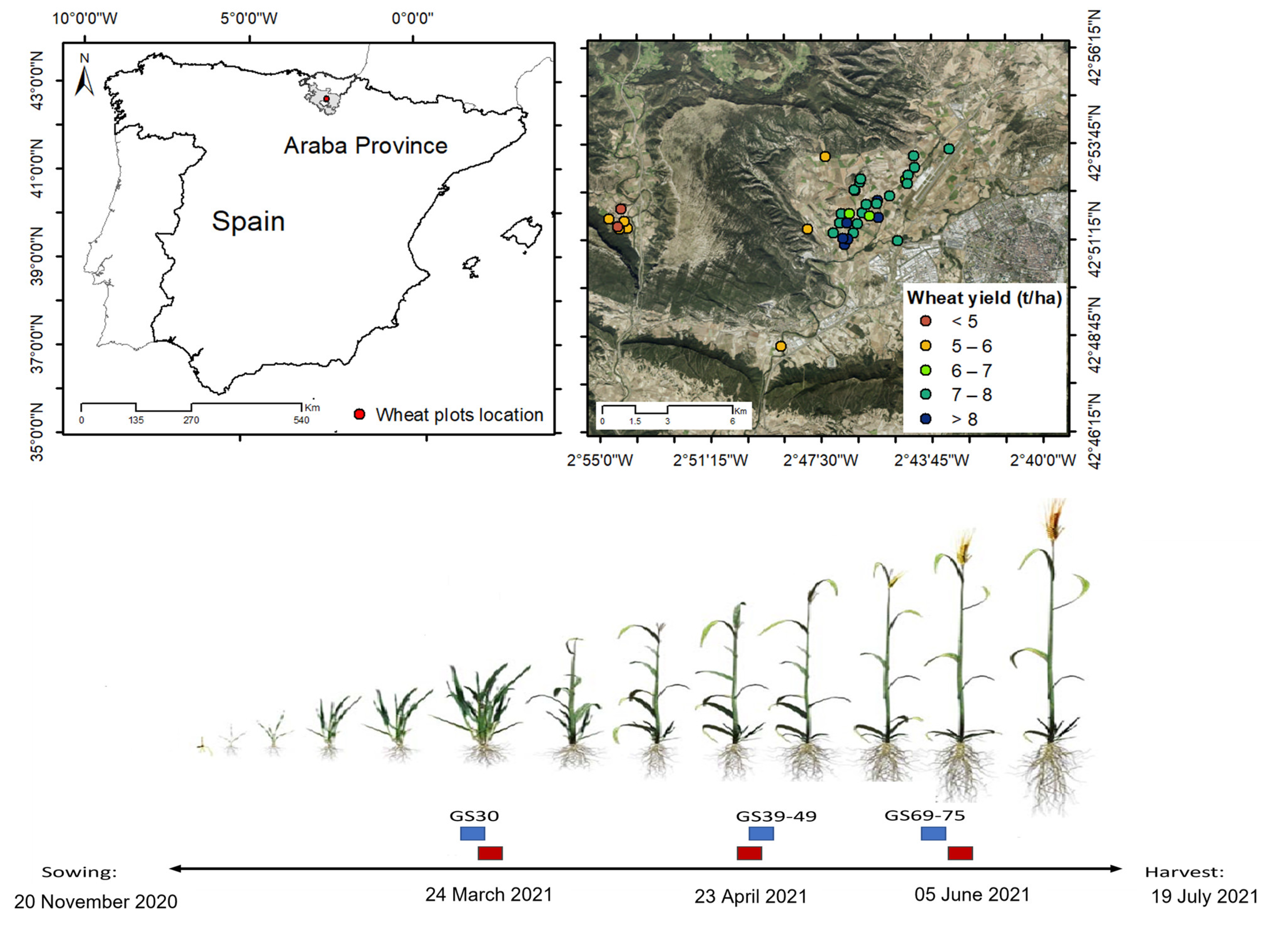
Figure 1. Upper left-hand side of the image shows the general location of the study area within Spain. Upper right-hand side shows detail of the study area with the average yield of each plot (right part). Below, wheat phenological stage and dates when satellite images were acquired. Red squares represent S1 and blue squares represent S2.
Remotesensing 15 01640 g001
Figure 2. Workflow followed for the pre-processing of S1 images to obtain backscatter information.
Remotesensing 15 01640 g002
Figure 3. Correlation matrix between the different VIs of the three days (Days 1–3). The last column shows the correlation with the wheat grain yield.
Remotesensing 15 01640 g003aRemotesensing 15 01640 g003b
Figure 4. R2 and RMSE of the four tested algorithms (MLR, Multiple Linear Model; RF, Random Forest; SVM, Support Vector Machine; CatBoost) when trained with VIs derived from S2 corresponding to different dates. It also shows accuracy metrics of the combination of different days.
Remotesensing 15 01640 g004
Figure 5. R2 and RMSE of the four algorithms (MLR, Multiple Linear Model; RF, Random Forest; SVM, Support Vector Machine; CatBoost) when trained with VV and VH polarization backscatter information derived from S1 corresponding to three different dates. It also shows their combined use.
Remotesensing 15 01640 g005
Figure 6. RMSE obtained using the CatBoost algorithm with data from S1 (Sentinel-1), S2 (Sentinel-2), and the combination of both (Sentinel-1 and Sentinel-2).
Remotesensing 15 01640 g006
Figure 7. Linear regression between observed and predicted wheat grain yield for the test dataset obtained using the CatBoost algorithm and the S1S2 dataset.
Remotesensing 15 01640 g007
Figure 8. The 10 variables from S1 and S2 that most contributed to the model.
Remotesensing 15 01640 g008
Figure 9. %MAE of the 39 plots when yield was predicted using the information from the rest of the plots. Those plots where %MAE is higher than 10% are shown in red. The dashed black line represents the mean %MAE.
Remotesensing 15 01640 g009
Figure 10. On the left, the classified wheat yield map of plot G15 (6.97 ha). On the right, classified wheat yield map based on the yield data estimated using the CatBoost algorithm with the S1S2 dataset for Days 1–3. The areas with low production are depicted in red, whereas those with high production are shown in blue. The accuracy and KI metrics were used to compare the two maps.
Remotesensing 15 01640 g010
Table 1. Vegetation indices calculated in this study with their formulae according to the S2 bands used.
Vegetation IndexAbbreviationFormulaReference
Normalized Difference
Vegetation Index
NDVI(B8 − B4)/(B8 + B4)[62]
Green Ratio Vegetation IndexGRVIB8/B3[63]
Green Normalized Difference Vegetation IndexGNDVI(B8 − B3)/(B8 + B3)[64]
Green Difference Vegetation IndexGDVIB8 − B3[65]
Enhanced Vegetation Index 2EVI22.4 × ((B8 − B4)/(B8 + B4 + 1))[66]
Chlorophyll Vegetation
Index
CVIB8 × (B4/(B3 × B3))[67]
Color IndexCI(B4 − B2)/B4[68]
Wide Dynamic Range
Vegetation Index
WDRVI((0.1 × B8) − B4)/((0.1 × B8) + B4)[69]
Transformed Vegetation
Index
TVI B 8 B 4 / B 8 + B 4 + 0.5 [70]
Soil Adjusted Vegetation
Index
SAVI((B8 − B4)/(B8 + B4 + 0.5)) × (1 + 0.5)[71]
Simple Ratio 800/670 Ratio Vegetation IndexRVIB8/B4[72]
Optimized Soil Adjusted Vegetation IndexOSAVI(1 + 0.16) × ((B8 − B4)/(B8 + B4 + 0.16))[73]
Nonlinear Vegetation IndexNLI((B8 × B8) − B4)/((B8 × B8) + B4)[74]
Table 2. Mean values of RMSE, SD and rRMSE of the four algorithms (MLR, Multiple Linear Model; RF, Random Forest; SVM, Support Vector Machine; CatBoost). Three different datasets were employed: S1 using only data from S1, S2 using data only from S2 and S1S2 using data from S1 and S2.
Algorithmn *Mean RMSE (t ha−1)SDrRMSE (%)
MLR301.10.7715.25
RF300.690.359.78
SVM300.620.348.92
CatBoost300.410.295.91
* Each algorithm was trained and tested with ten different partitions of each dataset (S1, S2 and S1S2).
Disclaimer/Publisher’s Note: The statements, opinions and data contained in all publications are solely those of the individual author(s) and contributor(s) and not of MDPI and/or the editor(s). MDPI and/or the editor(s) disclaim responsibility for any injury to people or property resulting from any ideas, methods, instructions or products referred to in the content.