Abstract
Hawkweeds (Pilosella spp.) have become a severe and rapidly invading weed in pasture lands and forest meadows of New Zealand. Detection of hawkweed infestations is essential for eradication and resource management at private and government levels. This study explores the potential of machine learning (ML) algorithms for detecting mouse-ear hawkweed (Pilosella officinarum) foliage and flowers from Unmanned Aerial Vehicle (UAV)-acquired multispectral (MS) images at various spatial resolutions. The performances of different ML algorithms, namely eXtreme Gradient Boosting (XGB), Support Vector Machine (SVM), Random Forest (RF), and K-nearest neighbours (KNN), were analysed in their capacity to detect hawkweed foliage and flowers using MS imagery. The imagery was obtained at numerous spatial resolutions from a highly infested study site located in the McKenzie Region of the South Island of New Zealand in January 2021. The spatial resolution of 0.65 cm/pixel (acquired at a flying height of 15 m above ground level) produced the highest overall testing and validation accuracy of 100% using the RF, KNN, and XGB models for detecting hawkweed flowers. In hawkweed foliage detection at the same resolution, the RF and XGB models achieved highest testing accuracy of 97%, while other models (KNN and SVM) achieved an overall model testing accuracy of 96% and 72%, respectively. The XGB model achieved the highest overall validation accuracy of 98%, while the other models (RF, KNN, and SVM) produced validation accuracies of 97%, 97%, and 80%, respectively. This proposed methodology may facilitate non-invasive detection efforts of mouse-ear hawkweed flowers and foliage in other naturalised areas, enabling land managers to optimise the use of UAV remote sensing technologies for better resource allocation.
1. Introduction
Weed control is essential for protecting biodiversity and for limiting impacts on yield loss and product quality in crops and pastures [1,2,3,4]. Conventional surveillance methods (e.g., field surveys) for invasive plant species are typically time-consuming, risky, and costly, resulting in a paucity of quantitative data regarding weed distribution in Australia [5]. Surveillance is a crucial aspect of biosecurity since it enables the early discovery of invasive species and develops an understanding of the spread of pests, weeds, and diseases. Remote sensing can efficiently and cost-effectively acquire geospatial data over expansive areas [6]. The combination of remote sensing and airborne imaging to assess weed populations is a technology that is expanding globally but remains in its infancy in many countries. Specifically, images acquired via the use of Unmanned Aerial Vehicles (UAVs) in recent years have proven their suitability for weed detection in different crops [5,7,8,9]. Most UAV-based remote sensing studies use Red, Green, Blue (RGB) sensors, which capture reflected light within the visible red, green, blue section of the electromagnetic spectrum for different applications. These sensors offer many advantages, including low cost, light weight, high spatial resolution, ease of use, simplicity of data processing, and reasonably low specifications for the working environment [10,11]. However, they are unable to capture light energy reflected in the non-visible segments of the electromagnetic spectrum, reducing the ability to discriminate between objects that appear similar to the human eye. Multispectral (MS) sensors offer a solution to this challenge, since they are capable of sensing radiation from both of invisible (red-edge and near-infrared) and visible segments of the spectrum, a region of four to six bands [12,13]. MS sensors have typically facilitated the accurate detection of crop health and diversity aiding decision making [14,15,16,17,18,19]. Despite the lower economic cost of imagery acquisition, RGB image processing tends to be insufficient for detecting weeds in their vegetative stages, when spectral signatures are less distinguishable from other green vegetation [10,20].
Mounting an UAV platform with a MS sensor is a very useful tool for performing crop and weed monitoring field studies at early phenological stages [21,22,23,24,25,26]. Further, the application of machine learning (ML) techniques and analysis to remotely sensed multispectral imaging has been identified as a potentially cost-effective strategy for locating diverse weed species [27] and has been typically used for remote vegetation mapping in different landscapes [28]. ML techniques have made it possible to extract the visible and invisible electromagnetic spectrum regions that can be employed for discrimination of different vegetation and non-vegetation [29]. The Vegetation Index (VI) is used to improve the accuracy of comparisons of plant growth and changes in canopy structure over time and in different regions by emphasizing the role of vegetation characteristics [30]. Combining ML techniques with a VI is a relatively new and advanced practice [31] that may be used to identify target weeds from surrounding vegetation at earlier phenological stages [32].
1.1. Hawkweed
Hawkweeds (Pilosella spp.) are perennial herbs that are serious environmental and agricultural weeds invading many temperate and subalpine areas of the world [33]. Hawkweeds are native to Europe and Asia [34] and have become major weeds in the United States of America, Canada, Japan, Australia, and New Zealand [35]. In New Zealand, hawkweeds have invaded more than 6 million ha of the South Island, particularly on the Canterbury Plains. Hawkweeds can spread quickly by seeds that are typically wind-dispersed and from stolon and root fragments [36]. Water, fodder, garden waste, and garden tools are also common hawkweed dispersal agents [37]. Hawkweeds have a unique appearance, featuring leaves up to 150 mm long that are green, arranged in a circular pattern near the ground and covered in delicate, long hairs. The stems have a milky sap and are covered in numerous short, rough bristly hairs [38]. Mouse-ear hawkweed (Pilosella officinarum) is a species characterised by a yellow flower with square-ended petals of up to 30 mm across, with a solitary flower on each stem. The species can quickly form dense mats, outcompeting neighbouring native and desirable species. It is also highly allelopathic, preventing the germination and growth of other plants by producing and secreting biochemicals into the surrounding soil [34]. Mouse-ear hawkweed poses a major threat to southeast Australia [34], and the lack of aerial detection techniques available currently severely limits de-limitation efforts. Small infestations exist in alpine areas of both Victoria and New South Wales and are eradication targets. Mouse-ear hawkweed has the potential to expand significantly beyond these regions under forecast climate scenarios [34,39]. The first step in any weed eradication program is to find the plant and delimit the infestation. In the case of mouse-ear hawkweed in NSW, the infestation exists in rugged and remote areas of Kosciuszko NP where ground survey is difficult and costly.
1.2. Machine Learning Models for Weed Detection
Recent research highlights several methods used to create weed maps from UAV images. The random forest (RF) classifier is gaining popularity in remote sensing due to its versatility, speed, and efficiency, making it a desirable choice for classifying high-resolution drone images and mapping agriculture [40]. The support vector machine (SVM) is another popular ML classifier which has been used for the classification of weeds [40] and is among the most prominent of ML techniques utilised for pattern recognition and regression. It has been characterised as unique and faster than other ML techniques [41] and can effectively handle large volumes of data [33]. eXtreme Gradient Boosting (XGB) is a class of ensemble ML classification techniques that can be used as an effective gradient-boosting implementation for predictive regression modelling [42]. K-nearest neighbours (KNN) is also a prevalent ML algorithm that performs well in supervised learning scenarios and simple recognition issues [41,42].
Several studies have successfully reported the use of these models for the detection of weed species (Table 1). In one study, three ML models, namely RF, SVM, and KNN, were employed to detect weeds in chili farms, resulting in an overall accuracy of RF—96%, KNN—63%, and SVM—94% [43]. Back-propagation neural networks (BPNNs), a specific type of Artificial Neural Network (ANN), and SVMs were utilised in weed detection in soybean fields in another study, resulting in an accuracy of BPNN—96.6% and SVM—95.7% [44]. Real-time weed detection was performed using RF with an accuracy of 95% in another study [45]. The classification of weeds was carried out using SVM with an overall accuracy of 97% in a different study [46]. Similarly, the detection of weeds in sugar beet fields was performed using ANN and SVM with an accuracy of ANN—92.9% and SVM—95% [47]. Weed mapping was also carried out using both Supervised Kohonen Network (SKN) and ANN with an overall accuracy of SKN—99% and ANN—99% [48]. Another study, conducted in Morocco, used ML and multispectral UAV data to detect weeds in a citrus farm. The study found that the RF classifier was more robust than KNN in classifying the weeds [49]. Another study utilised ML and UAV multispectral imagery to conduct spectral analysis and map blackgrass weed, achieving high accuracy rates using the RF classifier of 94%, 94%, and 93% [50]. Most of the above studies obtained good overall accuracy in detecting different weeds. Therefore, this study focuses on frequently used ML models for detecting hawkweed.

Table 1.
Application of machine learning techniques for weed detection.
To date, several studies associated with the analysis of imagery to detect hawkweeds have been undertaken around the globe. A program to detect orange hawkweed (Pilosella aurantiaca) flowers by manually viewing and logging pixel values was recently developed, but no ML model was used in the study [26]. Other studies have compared the detection of yellow hawkweed (Pilosella caespitosa) with high-resolution multispectral digital imagery to using supervised and unsupervised classification techniques [51]. However, classification methods exhibited low accuracy for detecting yellow hawkweed at lower ground cover percentages, possibly due to mixing with other grasses, making detection difficult. Calvin and Salah (2015) [52] also conducted research on surveillance systems for orange hawkweed detection using different spatial resolutions. Results showed that at 30 m above ground level (AGL), the flowers were represented by a small number of pixels and significant pixel mixing occurred, reducing the performance of the detection algorithm. Other studies have developed a spectral library for weed species in alpine vegetation communities, highlighting the potential to map orange and mouse-ear hawkweed based on their spectral characteristics [53].
Recently, remote sensing methods (i.e., RGB sensors mounted on aerial platforms) have been successfully utilised to detect orange hawkweed flowers in Kosciuszko National Park, Australia [54]. However, there is a need to determine an effective ML approach for the detection of mouse ear hawkweed, due to the significant threat this species poses on Australian alpine regions into the future. This study thus proposes an optimal technique for detecting mouse-ear hawkweed flowers (model 1) and foliage (model 2) in UAV acquired MS imagery and compares different ML classification algorithms at different spatial resolutions. The reason for developing two separate models for detecting mouse-ear hawkweed, one for flowers (model 1) and the other for foliage (model 2), is to ensure year-round applicability. A single model for detecting both flower and foliage may not be suitable for non-flowering seasons, leading to lower detection accuracy. Therefore, two models were developed to address this limitation. By having separate models for flowers and foliage, our approach allows for accurate detection of mouse-ear hawkweed at any time of the year. The specific objectives of this study were to: (1) correlate the vegetation indices with the hawkweed diversity; (2) evaluate the performance of different ML models to detect mouse ear hawkweed foliage and flowers; and (3) compare the accuracy of models in different spatial resolutions. The outcomes of this study may ultimately support effective weed biosecurity and management in regions invaded by this species within Australia and across the world by providing a mechanism to greatly enhance surveillance and facilitate accelerated eradication.
2. Materials and Methods
2.1. Site Description
Due to a paucity of mouse-ear hawkweed present in Australia and it being under active eradication, a large hawkweed infestation in New Zealand was chosen as the study site, thereby providing a sufficient quantity of data. All imagery was obtained at Sawdon Station in the McKenzie Region, south of Lake Tekapo, New Zealand (44°8’39.17”S and 170°18’30.80”E) in January 2021, as shown in Figure 1. Sawdon Station is a 7500 ha high country property, consisting of pastures used for sheep grazing. All imagery was captured in three 1–2 ha areas which included a high, medium, and low density level of mouse-ear hawkweed. The capture area was a floristically simple grassland where mouse-ear hawkweed was co-dominant with several grass species.
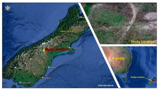
Figure 1.
Study site location at Sawdon Station, New Zealand (EPSG:4326—WGS 84).
2.2. Ground Truthing
To assist in the confirmation of mouse-ear hawkweed captured in the imagery, blue ropes were positioned across the site to demarcate areas of varying hawkweed density, providing regions of known species location (Figure 2). Botanical descriptions of mouse-ear hawkweed and other vegetation and the degree of ground disturbance within each section were recorded. High resolution ground photos were also taken to assist reliably identify hawkweed in the aerial imagery. Ground truth locations from 3, 4, 6, 10, and 11 (large patches) were selected for training and ground truth locations from 1, 2, 5, 7, 8, 9, 12, and 13 (small patches) were selected for validating the model. In addition, weather data, including cloud cover, wind velocity, humidity, temperature, and altitude were also recorded prior to imagery acquisition.
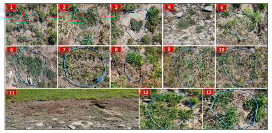
Figure 2.
Images 1 to 13 show each of the sectioned areas used for ground truth data collection at the study site.
2.3. Collection of Multispectral UAV Images
The UAV flight missions were conducted using a Micasense Altum multispectral camera (MicaSense, Inc., Washington, DC, USA) mounted on a DJI Matrice 600 (Da-Jiang Innovations (DJI), Shenzhen, Guangdong, China) UAV between 12:00 and 14:00 NZ local time on 30 January 2021 under sunny conditions. The Altum camera captures five radiance bands in the visible and near infrared regions (i.e., Blue, Green, Red, Red Edge, and Near Infrared) comprising wavelengths of 475.0 nm, 560.0 nm, 668.0 nm, 717.0 nm, and 842.0 nm, respectively. The Altum has a horizontal resolution of 2064 pixels, a vertical resolution of 1544 pixels, a sensor width of 7.12 mm, and a sensor height of 5.33 mm. The focal length of the camera is 8.0 mm, and the shutter interval is of 1 s. In order to obtain multispectral images in reflectance, sample images before and after each flight were taken by pointing the camera to a calibrated reflectance panel (CRP), which is provided by the sensor manufacturer. Calibration coefficients to convert the images from radiance to reflectance were obtained from the resulting images using Mica sense’s CRP processing tool, and these coefficients were applied to the target area images to ensure accurate and consistent reflectance measurements. The flight missions were conducted and recorded at the altitudes, resolutions, flight speeds, and take-off times, shown in Table 2, (AGL: 15–45 m, GSD: 0.65 to 1.95 cm/pixel, drone speed: 2 to 5 m/s, front overlap: 75%, take-off times: 12.10 to 13.35) to determine the ideal resolution for the detection of mouse-ear hawkweed, being cognizant that lower-resolution imagery is cheaper to collect and allows greater areas to be surveyed. Flight planning enabled the UAV to capture data using lawn mower patterns as illustrated in Figure 3.
Table 2.
Summary of multispectral flight mission data acquired at Sawdon Station hawkweed study site on 30 January 2021.
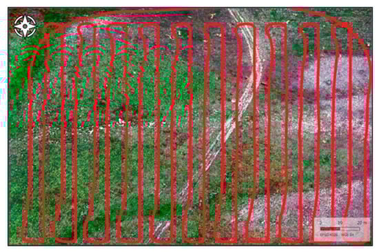
Figure 3.
Lawn mower pattern of UAV mission (EPSG:4326—WGS 84).
2.4. Software and Python Libraries
Several software applications and Python libraries were used to manage the ac-quired data. For multispectral image analysis, Agisoft Metashape 1.6.6 (Agisoft LLC, Petersburg, Russia) was used to process, filter, and orthorectify images. A collection of images was recovered from cropped sections and then labelled using QGIS (Version 3.2.0; Open-Source, Geospatial Foundation, Chicago, IL, USA). ENVI 5.5.1 (Environment for Visualizing Imagery, 2018, L3Harris Geospatial Solutions Inc, Broomfield, CO, USA) was used to apply different filters to reduce the noise in the multispectral image. Visual Studio Code (VS Code 1.70.0, Microsoft Corporation, Washington, DC, USA) was utilised as the source code editor for the development of ML algorithms using Python software (version 3.8.10, Python Software Foundation, Wilmington, DE, USA). Several libraries were utilised for data processing and ML, including Geospatial Data Abstraction Library (GDAL) 3.0.2, eXtreme Gradient Boosting (XGBoost) 1.5.0, Scikit-learn 0.24.2, OpenCV 4.6.0.66, and Matplotlib 3.0.
2.5. Orthomosaics and Raster Alignment
Initial image processing consisted of the development of different orthomosaics at all flight missions for same site. Orthomosaics resulting from various flight missions, namely GSD at 0.86, 1.10, 1.30, 1.50, 1.73, and 1.95 cm/pixel, were georeferenced with the highest resolution raster image (0.65 cm/pixel) by the pixel-level alignment technique. This technique was important to avoid manual image annotation for all flight missions and is described in Section 2.7. The georeferencing technique was utilised to save time during the labelling process.
2.6. Region of Interest (ROI) for Training and Validation
In accordance with the ground truth locations depicted in Figure 2, the orthomosaic was cropped into thirteen (13) ROIs for labelling the training dataset and the validation dataset.
2.7. Raster Labelling
QGIS was utilised to label both the training and validation datasets. For developing the hawkweed flower detection model (model 1), a mask for each image was built to conduct image labelling by assigning integer values to each highlighted pixel including 1 = Hawkweed flower, 2 = Non hawkweed flowers or background (including hawkweed foliage, other vegetation, and non-vegetation). Another model for detecting hawkweed foliage (model 2) was also developed using 3 classes (1 = hawkweed foliage (target vegetation), 2 = other vegetation, 3 = non vegetation). Using the toggling/editing function and adding polygon tools in QGIS, a new shapefile was generated to label each class with polygons drawn on the MS orthomosaic image. Figure 4 depicts an example of labelled hawkweed foliage in the ground truth location (ROI) number 11.
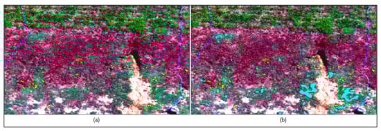
Figure 4.
Ground truth labelling for hawkweed foliage detection model: (a) Actual multispectral image, (b) Polygon labelling over hawkweed foliage (EPSG:4326—WGS 84).
2.8. Statistical Analysis for Algorithm Development
Two statistical analyses of multicollinearity testing, and normality testing were conducted to develop the ML models before loading the input features (five bands and VIs). Initially, sixteen vegetation indices (VIs) were considered for building machine learning models, but only six were chosen after conducting a multicollinearity test using the variable inflation factors (VIF) to prevent overfitting. The VIF was applied to assess the increase in variance of the estimated regression coefficient if the independent variables were correlated. A normality test was performed to confirm that the sample data came from a normally distributed population for developing the ML models.
2.9. Development of Classification Algorithms and Prediction
Numerous processes are involved in constructing algorithms, including loading, pre-processing especially annotation, fitting the classifier to the data, prediction, and validation. The processing phase transforms the read input into a set of features, which the classifier subsequently analyses. MS images (with five reflectance bands) were applied to a low pass filter for image smoothing through decreasing the disparity between pixel values by averaging nearby pixels using ENVI for accurate detection before importing into the algorithm. The different VIs were estimated to develop and improve the models in this study. Only six vegetation indices were chosen to develop the ML models for detecting hawkweed foliage and flowers based on the outcomes of multicollinearity testing to overcome the overfitting of the model. Then, five reflectance bands were loaded into the algorithm to increase detection rates by calculating spectral vegetation indices (VI). The Normalised Difference Vegetation Index (NDVI), Green Normalised Vegetation Index (GNDVI), Normalised Difference Red Edge Index (NDRE), Green Chlorophyll Index (GCI), Modified Soil-Adjusted Vegetation Index (MSAVI), and Excess Green (ExG) were selected and calculated to improve the input features and accuracy of the models, as shown in Table 3 and Figure 5.
Table 3.
Estimation of vegetation indices for model development.
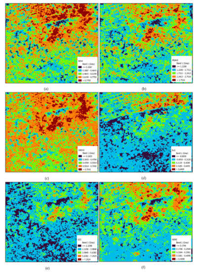
Figure 5.
Vegetation Indices (EPSG:4326—WGS 84) (a) NDVI; (b) MASVI; (c) GNDVI; (d) ExG; (e) GCI; (f) NDRE.
All five reflectance bands and the computed VIs were used as input features. The labelled regions were exported from QGIS. The majority class of non-hawkweed flowers (including hawkweed foliage, other vegetation, and non-vegetation) is more likely to be over-classified due to its higher prior probability, leading to misclassification of instances from the minority class (hawkweed flowers) during hawkweed flower detection model development due to imbalance dataset. Therefore, the data level resampling technique [64] was performed to modify the training set to make it suitable for a ML algorithm [65]. After resampling, the dataset was placed into an array and filtered pixel-wise data were randomly divided into a training array (75%) and a testing array (25%). Initially, the highest resolution raster dataset (15 m) was fitted into many ML classifiers, including XGB, SVM, RF, and KNN, to detect the hawkweed foliage and flowers at the site. The best ML model was subsequently chosen based on the highest model accuracy. The selected ML model was utilised for training all other resolutions, using the same labelled vector file generated by the highest resolution and using the georeferencing technique. K-fold cross-validation (K-fold: 10) was then utilised to evaluate the performance of the model. In the prediction phase, unlabeled pixels were processed using the best performing classifier and displayed in the same 2D spatial image from the orthorectified multispectral data. The identified pixels from each image were then assigned different colors and saved in TIF format for use with Geographic Information Systems (GIS) software. Finally, the predicted map was aligned with the actual multispectral raster and the accuracy of the expected outcome was confirmed by weed specialists using the model validation accuracy and ground truth verification that were mentioned in Section 3.1 and Section 3.2.
2.10. Classification Report
The labelled pixels from the multispectral image were fed into a ML model to detect the hawkweed foliage and flower and map the spatial distribution of hawkweed diversity in the study site. Overall model accuracy and precision were used to evaluate the model’s validation performance for detection of mouse-ear hawkweed flowers and foliage. Confusion matrix and classification reports were established to compare and evaluate the detection performance of the models. Evaluation descriptors, including true positive (TP), false positive (FP), true negative (TN), and false-negative (FN), were used to construct the confusion matrix (Equation (1)) and to determine the overall accuracy (Equation (2)), precision (Equation (3)), recall (Equation (4)), and F1 score (Equation (5)).
2.11. Data Processing Pipeline
Figure 6 depicts the development of a process pipeline with five components: acquisition, pre-processing, training, assessment, and prediction. Images are gathered, orthorectified, and pre-processed to obtain training samples with critical properties, which are subsequently labelled. The information is then forwarded to ML classifiers, trained, and optimised for detection.
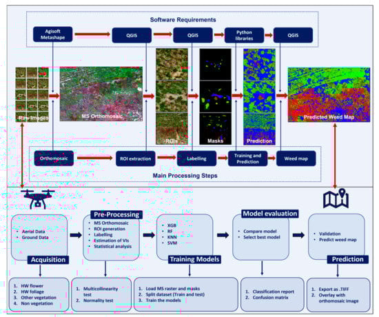
Figure 6.
UAV-acquired multispectral imagery processing pipeline for detection models.
3. Results
3.1. Detection of Hawkweed Flowers (Model 1)
Two accuracy matrices including model testing accuracy generated during the training process and model validation accuracy generated using best model and ground truth verification were also conducted to evaluate and verify the prediction results from selected ML model at selected spatial resolution for the detection of hawkweed flowers.
3.1.1. Model Testing Accuracy
Results of the analysis showed an overall model testing accuracy of 100% was attained with XGB, RF, and KNN to detect mouse-ear hawkweed flower at the study site. However, SVM, obtaining an overall accuracy of 99%, as shown in Table 4. All four models performed well in classifying instances into the hawkweed flowers and background (non-hawkweed flowers) classes, with perfect precision, recall, and F1 score (Table 5). Based on the confusion matrices (Figure 7), it appears that all four models displayed high accuracy in classifying instances into two classes: hawkweed flowers and background. Indeed, all models achieved a high number of true positives and true negatives, and the number of false positives and false negatives were minimal. It is worth noting that the SVM model had slightly more false positives than the other models, but the overall performance of all models was strong during testing.
Table 4.
Overall testing accuracy of different machine learning models for detection of hawkweed flowers at 0.65 cm/pixel.
Table 5.
Classification report (testing) of different machine learning models for detection of hawkweed flowers at 0.65 cm/pixel.
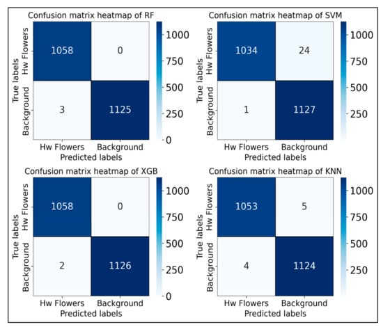
Figure 7.
Confusion matrix for training of different machine learning models for flower detection.
Finally, the XGB model was selected as the best model to train the other resolution imagery for detection of hawkweed flowers as shown in Table 6, since XGB took the shortest training time in comparison to other models. As expected, the 0.65 cm/pixel (15 m AGL) mission obtained the highest overall accuracy (100%) for detection of hawkweed flowers than any other ground sampling distance in the study site. Different region of interests (ROIs) at the ground truth location number 11 were used to train the model for detection of hawkweed flowers in the study site due to the high density of hawkweed flowers in this location. Figure 8 shows the XGB model prediction results during training. Hawkweed flowers are predicted as a yellow highlight and black background depicts the other regions in the training site not containing hawkweed flowers.
Table 6.
Overall testing accuracy report of XGB for different spatial resolutions at the study site.
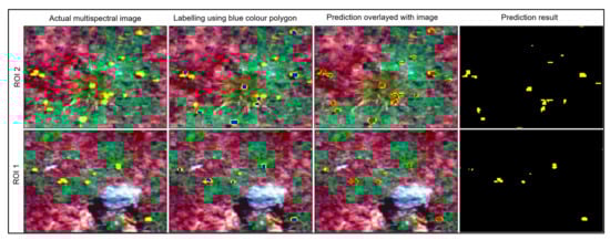
Figure 8.
Training at ground truth location number 11 (ROI-1, 2) using XGB model (EPSG:4326—WGS 84).
3.1.2. Model Validation Accuracy
Different ROIs at the ground truth location number 11 (at 0.65 cm/pixel) were used to validate the model for detection of hawkweed flowers in the study site. Results of the analysis show an overall model validation accuracy of 100% using the XGB, RF, and KNN model to detect mouse-ear hawkweed flowers at the study site (Table 7). All models achieved high precision and F1 score for both classes. However, RF, KNN, and XGB models achieved 100% of precision, recall and F1 score for detection of hawkweed flowers. While the SVM model achieved slightly lower recall and F1 score for the hawkweed flowers and background class (Table 8). In general, all models performed well and achieved high accuracy in classifying the hawkweed flowers and background pixels.
Table 7.
Overall validation accuracy of different machine learning models for detection of hawkweed flowers at 0.65 cm/pixel.
Table 8.
Classification report (validation) of different machine learning models for detection of hawkweed flowers at 0.65 cm/pixel.
Based on the confusion matrices (Figure 9), it appears that all four models had high accuracy in classifying instances into two classes: hawkweed flowers and background. In fact, all models achieved a high number of true positives and true negatives, and the number of false positives and false negatives were minimal. It is worth noting that the SVM model had slightly more false positives than the other models, but the overall performance of all models was strong. These findings suggest that any of these four models may be effective in classifying instances of hawkweed flowers and background. Figure 10 shows the prediction results at the validation site and most of the hawkweed flowers were detected using this model during the validation process.
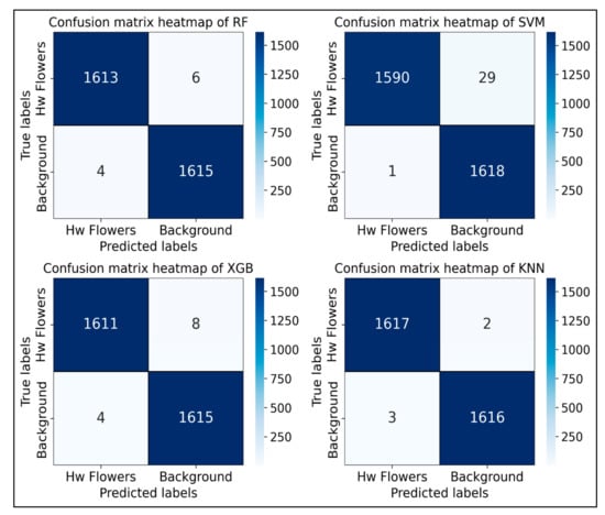
Figure 9.
Confusion matrix for validation of different machine learning models for flower detection.
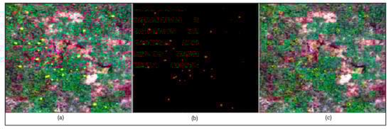
Figure 10.
Validation at ground truth location number 11 (a) Actual multispectral image; (b) Prediction result; (c) Prediction results are overlayed with actual image (EPSG:4326—WGS 84).
3.1.3. Ground Truth Verification
After completing the model validation, verification was conducted by weed specialists by comparing the ground truth ROIs extracted from multispectral orthomosaic and pixelwise prediction results to verify the model performance (Figure 11).
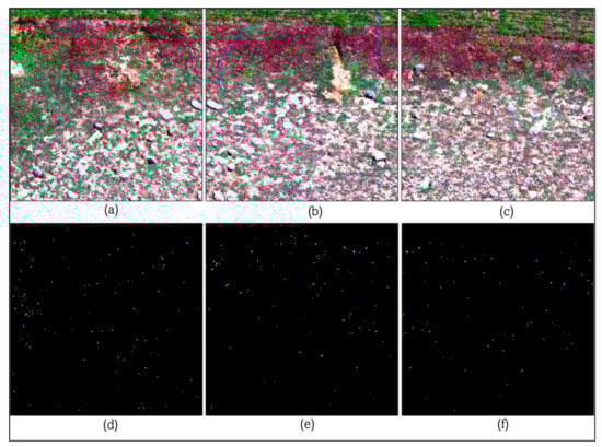
Figure 11.
Prediction results (EPSG:4326—WGS 84) (d–f) of XGB model within a large area of the study site for (a), (b), and (c) respectively.
3.2. Detection of Hawkweed Foliage (Model 2)
Just as in Section 3.1, model testing accuracy, model validation accuracy, and ground truth verification were applied to verify the prediction results from selected ML model at selected spatial resolution for the detection of hawkweed foliage.
3.2.1. Model Testing Accuracy
Table 9 displays the overall testing accuracy of four different machine learning models for detecting mouse ear hawkweed foliage (XGB, SVM, RF, and KNN) at a resolution of 0.65 cm/pixel at the study site. XGB and RF achieved the highest accuracy rates of 97%, while KNN achieved a slightly lower accuracy rate of 96%. SVM had the lowest accuracy rate of 72%. Table 10 presents the classification report of different machine learning models for the detection of hawkweed flowers at a resolution of 0.65 cm/pixel during validation. In relation to the detection of hawkweed class, RF, KNN, and XGB all achieved perfect precision, indicating that all the predicted hawkweeds were true positives. The models also had high recall rates, with values ranging from 94% to 100%, indicating that they were able to identify most of the actual hawkweeds present in the predicted image. All the models achieved F1 scores of 97% or above, indicating high overall performance. For the detection of other vegetation, all the models achieved relatively high precision rates ranging from 91% to 91%. However, the recall rates were lower, ranging from 41% to 100%, indicating that the models had some difficulty in correctly identifying all the other vegetation in the image. As a result, the F1 scores for this class ranged from 52% to 95%. For non-vegetation areas, all models achieved perfect precision and recall rates of 100% and 96%, respectively, indicating that they were able to accurately identify all non-vegetation areas in the image. The F1 scores for this class ranged from 98% to 89%.
Table 9.
Overall testing accuracy of different machine learning models for detection of mouse ear hawk-weed foliage at 0.65 cm/pixel at the study site.
Table 10.
Classification report (testing) of different machine learning models for detection of hawkweed foliage at 0.65 cm/pixel.
Table 11 displays the overall testing accuracy report obtained using the XGB model to detect hawkweed foliage at different spatial resolutions at a particular study site. The table lists the flight numbers, Ground Sampling Distance (GSD) in cm/pixel, and overall testing accuracy percentage for each flight. The table indicates that the XGB model performed well across all flight numbers and GSDs, achieving high overall testing accuracy percentages ranging from 91% to 97%. Flights 1 and 2, which had GSDs of 0.65 cm/pixel and 0.86 cm/pixel, respectively, achieved the highest overall testing accuracy percentages of 97%. Flight 3, which had a GSD of 1.10 cm/pixel, had a slightly lower accuracy rate of 95%, followed by flights 4 and 5 with GSDs of 1.30 cm/pixel and 1.50 cm/pixel, respectively, which both achieved overall testing accuracy percentages of 94%. Flights 6 and 7, which had larger GSDs of 1.73 cm/pixel and 1.95 cm/pixel, respectively, had lower overall testing accuracy percentages of 92% and 91%, respectively.
Table 11.
Overall testing accuracy report arising from the use of the XGB model to detect hawkweed foliage at different spatial resolutions at the study site.
The set of confusion matrices (as shown in Figure 12) displays the performance of four ML models, namely RF, SVM, XGB, and KNN, in classifying data into three classes. The numbers in each cell of the matrix represent the number of samples that were classified as a particular class. For example, in the RF confusion matrix, the number 7662 in the top-left cell indicates that 7662 samples were correctly classified as belonging to the target vegetation of hawkweed foliage. The number 516 in the second cell of the first row indicates that 516 samples that belong to the hawkweed foliage class were incorrectly classified as belonging to the other vegetation class. By analyzing the confusion matrices of the different models, one can determine which model has the highest accuracy rate in correctly classifying the samples into their respective classes. For example, in the RF and XGB models, the confusion matrices are identical, indicating that they have the same performance. Both models have high accuracy rates for all three classes, with very few incorrectly classified samples. The KNN model has a similar performance to the RF and XGB models but has slightly more incorrectly classified samples in the first class. The SVM model has the lowest accuracy rate among the four models, with more incorrectly classified samples in all three classes.
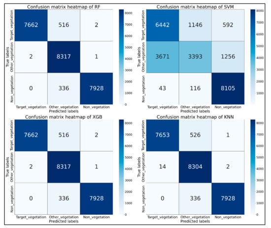
Figure 12.
Confusion matrix for training of different machine learning models for foliage detection.
Figure 13 illustrates the prediction results from different ML models in different ROIs (3, 4, 6, 10, 11) in the field and their respective masks. It clearly shows that RF, XGB, and KNN accurately detected the hawkweed foliage in the ROIs, while SVM predictions were poorer than those of the other models during training.
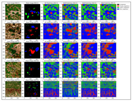
Figure 13.
Prediction results from training in different ground truth locations (ROIs) using different machine learning models.
3.2.2. Model Validation Accuracy
Different ground truth location numbers (ROI-1,2,5,7,8,9,12,13 at 0.65 cm/pixel) were used to validate the models for detection of hawkweed foliage in the study site. Table 12 provides information on the overall validation accuracy of four different ML models for detecting mouse ear hawk-weed foliage at 0.65 cm/pixel at the study site. The models compared are XGB, SVM, RF, and KNN. The accuracy values for the models are as follows: XGB-98%, SVM-80%, RF-97%, and KNN-97%. Table 13 provides a detailed classification report for the different machine learning models used to detect hawkweed flowers at a resolution of 0.65 cm/pixel during validation. The report includes precision, recall, and F1 score values for hawkweed, other vegetation, and non-vegetation, calculated as percentages. For hawkweed detection, the highest precision of 95% was achieved by the XGB model, followed by RF and KNN with 94%, and SVM with 54%. The highest recall of 96% was achieved by XGB and KNN, followed by RF and SVM with 94% and 81%, respectively. The highest F1 score of 95% was achieved by XGB and KNN, followed by RF and SVM with 94% and 65%, respectively. For other vegetation detection, the highest precision of 97% was achieved by RF and KNN, followed by XGB and SVM with 96% and 77%, respectively. The highest recall of 97% was achieved by all four models. The highest F1 score of 97% was achieved by RF and XGB, followed by KNN and SVM with 96% and 63%, respectively. For non-vegetation detection, all models achieved perfect precision, recall, and F1 score values of 100%. This indicates that all models correctly identified non-vegetation pixels without any false positives or false negatives.
Table 12.
Overall validation accuracy of different machine learning models for detection of mouse ear hawkweed foliage at 0.65 cm/pixel at the study site.
Table 13.
Classification report (validation) of different machine learning models for detection of hawkweed foliage at 0.65 cm/pixel.
This confusion matrix (Figure 14) shows the results of the four different ML models used for the detection of target vegetation (hawkweed foliage), other vegetation, and non-vegetation. For the hawkweed foliage class, all models had high true positive values, with RF having the highest number of true positives (23,035) and SVM having the lowest number (19,805). SVM had the highest false positive value for this class (4655), which means that it incorrectly classified some other vegetation or non-vegetation pixels as hawkweed foliage. RF had the lowest false positive value for this class (1431). For the other vegetation class, all models had high true positive values, with XGB having the highest number of true positives (23,661) and SVM having the lowest number (12,848). SVM had the highest false positive value for this class (420), which means that it incorrectly classified some hawkweed or non-vegetation pixels as other vegetation. RF had the lowest false positive value for this class (1133). For the non-vegetation class, all models had perfect true positive values, meaning they correctly classified all non-vegetation pixels. SVM had the highest false positive value for this class (6), which means that it incorrectly classified a small number of other vegetation or hawkweed pixels as non-vegetation. In terms of overall performance, RF and XGB had the highest number of true positives for all classes, while SVM had the highest number of false positives for hawkweed and other vegetation classes. KNN had similar performance to RF for all classes, with slightly lower true positive values for hawkweed and other vegetation.
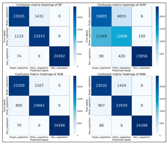
Figure 14.
Confusion matrix for validation of different machine learning models for foliage detection.
Figure 15 demonstrates how various ML models predicted hawkweed foliage in distinct regions of interest (ROIs 1, 2, 5, 7, 8, 9) in the field during validation, along with their corresponding masks. The results indicate that RF, XGB, and KNN accurately identified hawkweed foliage in the training ROIs, while SVM exhibited poorer predictive performance compared to the other models. After completing the model validation, verification was conducted by weed specialists to confirm the model performance and pixelwise prediction results.
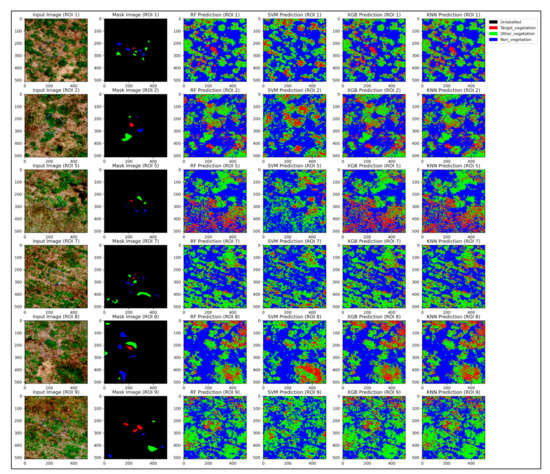
Figure 15.
Prediction results from validation in different ground truth locations (ROIs) using different machine learning models.
3.2.3. Prediction Results for Different Region of Interests at the Study Site
Figure 16 represents the model segmentation results with classes of hawkweed foliage, other vegetation, and non-vegetation at different GSD at a resolution of 0.65 cm/pixel using the XGB model. According to the prediction results as shown in Figure 16, hawkweeds were truly predicted in the pastureland (Figure 16d–f). Further, most of the pixels from hawkweed foliage were accurately predicted in Figure 16d,g because of limited mixing of hawkweed foliage and other vegetation. Hence, hawkweed foliage can be accurately detected where hawkweeds were grown in non-vegetation sites.
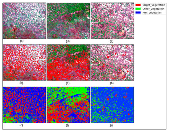
Figure 16.
Prediction results at different region of interest (EPSG:4326—WGS 84) (a,d,g)—Different region of study sites; (b,e,h)—Prediction result of hawkweed foliage; (c,f,i)—Prediction results of all classes (Hawkweed foliage, other vegetation, and non-vegetation.
4. Discussion
The results of this study show that MS sensors installed on UAVs are highly effective for detecting mouse-ear hawkweeds in their flowering stage in the grazing landscape. When applying ML models to remotely sensed data, the results further demonstrate the importance of spatial image resolution to image clarity and detection accuracy. Due to the expensive nature of high-resolution data acquisition, it remains necessary to identify models capable of enhancing image quality and recognizing species in lower-resolution imaging. The preliminary model accuracy matrix for the ML model in this study highlights the need for further validation regarding the prediction accuracy of models for detecting mouse ear hawkweed inhabiting a broader range of vegetation. This could be achieved by trialing the model within a different natural context in Australia (where mouse-ear hawkweed is present at lower densities). VIs have been shown to be useful in discriminating between different vegetation types because VIs are significantly correlated with different pigment concentrations in different vegetation. VIs represent a promising development towards automating the analysis of remote sensing images and the development of weed maps.
In the hawkweed flower detection model (Model 1), the XGB, RF, and KNN models achieved 100% accuracy, and thereby correctly classified all flower images in the validation dataset. The Support Vector Machine (SVM) model achieved an accuracy of 98% and incorrectly classified 2% of the flower images. The variation in accuracy values may be due to algorithm and parameter differences, as well as the quality and quantity of the training data available. For example, the XGB and RF models are ensemble models that combine multiple decision trees to improve accuracy, while the SVM and KNN models are based on different classification approaches. Additionally, the choice of hyperparameters, such as the number of trees in a RF or the number of neighbours in KNN, can affect the accuracy of the model. SVM is a sensitive model that requires careful tuning of its hyperparameters to achieve good performance. This is intuitive given the small size of the flowers relative to the pixel size. Therefore, UAV flight missions are recommended to capture minimum 0.65 to 0.86 cm/pixel GSD imagery for the detection of hawkweed flowers using the XGB model. In this study, the model accuracy was verified by a hawkweed specialist. They found only a few definitive false positives, but true verification was limited as only the very small areas covered by ground photos (quadrats) could be accurately verified. The aerial imagery was not of sufficient resolution to identify mouse-ear hawkweed flowers with high certainty. In the hawkweed foliage detection model (Model 2), XGB and RF seem to be the most suitable models for the given problem with the highest validation accuracy. Similarly, to model 1, it is evident that the greater number and smaller pixels (more detail) allows better definition of the hawkweed foliage against surrounding plants and features. The validation ROIs, as mentioned in Figure 15, were also verified by hawkweed specialists. According to the ground truth verification, most of the hawkweed foliage pixels were accurately detected. However, some were showing pixelwise misclassification due to overlapping of other vegetation with hawkweed foliage due to insufficient pixel size relative to the hawkweed plant and possibly the similarity of spectral values of other vegetation. Overall, the results suggest that the XGB and RF models will be the most accurate for detecting hawkweed foliage from multispectral imagery.
This study investigating the detection of mouse-ear hawkweed foliage and flowers in New Zealand from UAV-acquired multispectral imagery and ML algorithms makes a novel contribution to this field. Although other studies have also demonstrated the potential of ML algorithms in accurately detecting and classifying hawkweeds in Australia, several limitations still exist. One of these includes the absence of a ML model for detecting orange hawkweed flowers, which may make detection efforts of new infestations sub-optimal. Additionally, some classification methods employed in previous studies showed low accuracy in detecting yellow hawkweed, particularly at lower ground cover percentages, possibly due to the mixing of other grasses, which made detection difficult. Moreover, significant pixel mixing resulted from the use of different spatial resolutions in some studies, reducing, thus, the performance of the detection algorithm. Although a spectral library for weed species has been developed in Australian alpine vegetation communities, this method may not be feasible in other ecosystems or for different types of hawkweeds. In contrast, this study specifically focuses on the use of ML to detect hawkweed foliage and flowers, highlighting the advantages of this approach, such as achieving higher accuracy and the ability to automate the detection process. The study also provides detailed information on the specific ML techniques used. By using the RF, KNN, and XGB models, this study achieved a high overall testing and validation accuracy of 100% and 97%, respectively, in detecting hawkweed flowers at a spatial resolution of 0.65 cm/pixel. This high level of accuracy is a significant improvement compared to previous works [26,51,52,53].
This proposed methodology will provide opportunities for remote weed detection, with the ultimate goal of enabling land managers to target investment and optimise the use of available technologies to detect weeds in the landscape. The model can be used to detect hawkweed foliage and flowers in different flight missions and sites, supported effective weed biosecurity and management focused on building capacity and capability in remote weed detection, and provided learning opportunities on remote weed detection current practices and methods. There were a few limitations in this study. The unavailability of high-resolution RGB images for accurate labelling and the time and expertise required to label images accurately is a major hindrance. For small plants like mouse-ear hawkweed, accurate image tagging is difficult without high-resolution RGB imagery or paired ground photos. Although ground photos were available in the current study, they only covered a small portion of the aerial imagery capture, limiting certainty of image tagging and possibility of introducing errors at the outset. Another limitation included the colour or texture similarity of neighbouring species, presenting challenges for accurate labelling. This can lead to further time delays in workflow, presenting a problem with larger datasets. Furthermore, detection accuracy is influenced by the relatively simple floristics of the sampling area, e.g., in the current study, it was unknown if there were any other similar-coloured (yellow) flowers in the dataset and this created uncertainty as to the accuracy of labelling.
Ongoing work in the detection of hawkweeds is focused on overcoming existing ML model limitations via the application of DL techniques including object detection and semantic segmentation using convolutional neural networks (CNN). Since DL techniques offer considerable promise in this regard and are progressively being applied to weed detection due to their speed and accuracy, they are superior to those of conventional algorithms [66,67,68,69,70]. The tremendous success of DL methods used in image processing studies in recent years intersects with contemporary developments in UAV photogrammetry [21] with various DL techniques, showing great promise for the detection of a variety of weed species in different landscapes [70,71,72]. Future project work will continue to investigate remote sensing technologies and their application to additional environments, including; (1) Using handheld spectrophotometers to retrieve spectral information for each class in the field for more accurate labelling; (2) Collecting imagery encompassing a greater variety of habitat types (e.g., natural settings) to create a more robust model applicable to a broader range of mouse-ear hawkweed habitats; (3) Collecting temporal imagery to determine any reflectance differences of hawkweed relative to surrounding vegetation and possible increased accuracy, facilitating the ability to increase application of models in different contexts; and (4) Collection of hyperspectral imagery to improve model performance and more effectively differentiate between similar vegetative features. The use of UAVs for remote sensing purposes is still constrained by limitations in areas such as performance, cost, technology, and application scenarios. As a result, their contribution to practical grassland management decision-making processes is not yet satisfactory [66].
5. Conclusions
In summary, detecting and managing hawkweed infestations is critical for the conservation of pasture lands and forest meadows in New Zealand. This research explored the potential of classical ML algorithms to detect hawkweed foliage and flowers using multispectral imagery from UAVs at various spatial resolutions. The different VIs were estimated to develop and improve the models in this study. The study found that the RF, KNN, and XGB models could detect hawkweed flowers with high accuracy at a spatial resolution of 0.65 cm/pixel during training and validation. For hawkweed foliage detection, the RF and XGB models achieved the highest testing accuracy, while the XGB model achieved the highest overall validation accuracy. These findings highlight the potential of remote sensing and ML techniques in detecting hawkweeds in large areas, which could ultimately support effective weed biosecurity and management, enhancing surveillance and facilitating accelerated eradication. The proposed methodology could be implemented in other areas to facilitate the detection of hawkweed infestations, leading to better resource allocation and more efficient management.
Author Contributions
Writing—original draft preparation, N.A.; formal image analysis, investigation, N.A.; visualization, N.A.; image tagging and validation, M.H.; project administration, J.E.K. and H.C.; writing—review and editing, J.E.K., M.H., H.C., L.Z., R.L.D. and J.S.; supervision, F.G. and L.Z. All authors have read and agreed to the published version of the manuscript.
Funding
Data collection was supported by the NSW National Parks and Wildlife Service and the broader weed remote detection project by the Australian Department of Agriculture, Fisheries and Forestry.
Data Availability Statement
The data presented in this study are available on request from the project team members. The data are not publicly available due to the significant size of files.
Acknowledgments
The authors gratefully acknowledge the assistance of Rob Matthews and his team (Heli Surveys) in the acquisition of field data at the study sites.
Conflicts of Interest
The authors declare no conflict of interest.
References
- Luna, I.M.; Fernández-Quintanilla, C.; Dorado, J. Is Pasture Cropping a Valid Weed Management Tool? Plants 2020, 9, 135. [Google Scholar] [CrossRef]
- Cousens, R.; Heydel, F.; Giljohann, K.; Tackenberg, O.; Mesgaran, M.; Williams, N. Predicting the Dispersal of Hawkweeds (Hieracium aurantiacum and H. praealtum) in the Australian Alps. In Proceedings of the Eighteenth Australasian Weeds Conference, Melbourne, VIC, Australia, 8–11 October 2012; pp. 5–8. [Google Scholar]
- Rapinel, S.; Mony, C.; Lecoq, L.; Clément, B.; Thomas, A.; Hubert-Moy, L. Evaluation of Sentinel-2 time-series for mapping floodplain grassland plant communities. Remote Sens. Environ. 2019, 223, 115–129. [Google Scholar] [CrossRef]
- Rapinel, S.; Rossignol, N.; Hubert-Moy, L.; Bouzillé, J.-B.; Bonis, A. Mapping grassland plant communities using a fuzzy approach to address floristic and spectral uncertainty. Appl. Veg. Sci. 2018, 21, 678–693. [Google Scholar] [CrossRef]
- De Castro, A.I.; Torres-Sánchez, J.; Peña, J.M.; Jiménez-Brenes, F.M.; Csillik, O.; López-Granados, F. An Automatic Random Forest-OBIA Algorithm for Early Weed Mapping between and within Crop Rows Using UAV Imagery. Remote Sens. 2018, 10, 285. [Google Scholar] [CrossRef]
- Du, M.; Noguchi, N. Monitoring of Wheat Growth Status and Mapping of Wheat Yield’s within-Field Spatial Variations Using Color Images Acquired from UAV-camera System. Remote Sens. 2017, 9, 289. [Google Scholar] [CrossRef]
- Yano, I.H.; Alves, J.R.; Santiago, W.E.; Mederos, B.J. Identification of weeds in sugarcane fields through images taken by UAV and Random Forest classifier. IFAC-PapersOnLine 2016, 49, 415–420. [Google Scholar] [CrossRef]
- Barrero, O.; Perdomo, S.A. RGB and multispectral UAV image fusion for Gramineae weed detection in rice fields. Precis. Agric. 2018, 19, 809–822. [Google Scholar] [CrossRef]
- Peña, J.M.; Torres-Sánchez, J.; De Castro, A.I.; Kelly, M.; Lopez-Granados, F. Weed Mapping in Early-Season Maize Fields Using Object-Based Analysis of Unmanned Aerial Vehicle (UAV) Images. PLoS ONE 2013, 8, e77151. [Google Scholar] [CrossRef]
- Yang, G.; Liu, J.; Zhao, C.; Li, Z.; Huang, Y.; Yu, H.; Xu, B.; Yang, X.; Zhu, D.; Zhang, X.; et al. Unmanned Aerial Vehicle Remote Sensing for Field-Based Crop Phenotyping: Current Status and Perspectives. Front. Plant Sci. 2017, 8, 1111. [Google Scholar] [CrossRef]
- Amarasingam, N.; Gonzalez, F.; Salgadoe, A.S.A.; Sandino, J.; Powell, K. Detection of White Leaf Disease in Sugarcane Crops Using UAV-Derived RGB Imagery with Existing Deep Learning Models. Remote Sens. 2022, 14, 6137. [Google Scholar] [CrossRef]
- Arnold, T.; De Biasio, M.; Fritz, A.; Leitner, R. UAV-based multispectral environmental monitoring. In Proceedings of the SENSORS, Waikoloa, HI, USA, 1–4 November 2010; pp. 995–998. [Google Scholar] [CrossRef]
- Yao, H.; Qin, R.; Chen, X. Unmanned Aerial Vehicle for Remote Sensing Applications—A Review. Remote Sens. 2019, 11, 1443. [Google Scholar] [CrossRef]
- Rodríguez, J.; Lizarazo, I.; Prieto, F.; Angulo-Morales, V. Assessment of potato late blight from UAV-based multispectral imagery. Comput. Electron. Agric. 2021, 184, 106061. [Google Scholar] [CrossRef]
- Yang, W.; Xu, W.; Wu, C.; Zhu, B.; Chen, P.; Zhang, L.; Lan, Y. Cotton hail disaster classification based on drone multispectral images at the flowering and boll stage. Comput. Electron. Agric. 2021, 180, 105866. [Google Scholar] [CrossRef]
- Paredes, J.A.; Gonzalez, J.; Saito, C.; Flores, A. Multispectral Imaging System with UAV Integration Capabilities for Crop Analysis. In Proceedings of the IEEE 1st International Symposium on Geoscience and Remote Sensing, GRSS-CHILE, Valdivia, Chile, 15–16 June 2017. [Google Scholar] [CrossRef]
- Brinkhoff, J.; Vardanega, J.; Robson, A.J. Land Cover Classification of Nine Perennial Crops Using Sentinel-1 and -2 Data. Remote Sens. 2020, 12, 96. [Google Scholar] [CrossRef]
- Tu, Y.-H.; Johansen, K.; Phinn, S.; Robson, A. Measuring Canopy Structure and Condition Using Multi-Spectral UAS Imagery in a Horticultural Environment. Remote Sens. 2019, 11, 269. [Google Scholar] [CrossRef]
- Narmilan, A.; Gonzalez, F.; Salgadoe, A.S.A.; Powell, K. Detection of White Leaf Disease in Sugarcane Using Machine Learning Techniques over UAV Multispectral Images. Drones 2022, 6, 230. [Google Scholar] [CrossRef]
- Amarasingam, N.; Salgadoe, A.S.A.; Powell, K.; Gonzalez, L.F.; Natarajan, S. A review of UAV platforms, sensors, and applications for monitoring of sugarcane crops. Remote Sens. Appl. 2022, 26, 100712. [Google Scholar] [CrossRef]
- Khoshboresh-Masouleh, M.; Akhoondzadeh, M. Improving weed segmentation in sugar beet fields using potentials of multispectral unmanned aerial vehicle images and lightweight deep learning. J. Appl. Remote Sens. 2021, 15, 034510. [Google Scholar] [CrossRef]
- Kerkech, M.; Hafiane, A.; Canals, R. Vine disease detection in UAV multispectral images using optimized image registration and deep learning segmentation approach. Comput. Electron. Agric. 2020, 174, 105446. [Google Scholar] [CrossRef]
- Modica, G.; De Luca, G.; Messina, G.; Praticò, S. Comparison and assessment of different object-based classifications using machine learning algorithms and UAVs multispectral imagery: A case study in a citrus orchard and an onion crop. Eur. J. Remote Sens. 2021, 54, 431–460. [Google Scholar] [CrossRef]
- Banerjee, B.; Sharma, V.; Spangenberg, G.; Kant, S. Machine Learning Regression Analysis for Estimation of Crop Emergence Using Multispectral UAV Imagery. Remote Sens. 2021, 13, 2918. [Google Scholar] [CrossRef]
- Pérez-Ortiz, M.; Peña, J.M.; Gutiérrez, P.A.; Torres-Sánchez, J.; Hervás-Martínez, C.; López-Granados, F. Selecting patterns and features for between- and within- crop-row weed mapping using UAV-imagery. Expert Syst. Appl. 2016, 47, 85–94. [Google Scholar] [CrossRef]
- Hamilton, M.; Matthews, R.; Caldwell, J. Needle in a Haystack—Detecting Hawkweeds Using Drones. In Proceedings of the 21st Australasian Weeds Conference, Sydney, Australia, 9–13 September 2018; pp. 126–130. [Google Scholar]
- Etienne, A.; Saraswat, D. Machine learning approaches to automate weed detection by UAV based sensors. In Autonomous Air and Ground Sensing Systems for Agricultural Optimization and Phenotyping IV; SPIE: Bellingham, WA, USA, 2019; Volume 11008, p. 110080R. [Google Scholar] [CrossRef]
- Islam, N.; Rashid, M.; Wibowo, S.; Wasimi, S.; Morshed, A.; Xu, C.; Moore, S. Machine Learning Based Approach for Weed Detection in Chilli Field Using RGB Images. In Lecture Notes on Data Engineering and Communications Technologies; Springer Science and Business Media Deutschland GmbH: Berlin/Heidelberg, Germany, 2021; Volume 88, pp. 1097–1105. [Google Scholar] [CrossRef]
- Segarra, J.; Buchaillot, M.L.; Araus, J.L.; Kefauver, S.C. Remote Sensing for Precision Agriculture: Sentinel-2 Improved Features and Applications. Agronomy 2020, 10, 641. [Google Scholar] [CrossRef]
- Zhang, S.; Li, X.; Ba, Y.; Lyu, X.; Zhang, M.; Li, M. Banana Fusarium Wilt Disease Detection by Supervised and Unsupervised Methods from UAV-Based Multispectral Imagery. Remote Sens. 2022, 14, 1231. [Google Scholar] [CrossRef]
- Osco, L.P.; Ramos, A.P.M.; Pereira, D.R.; Moriya, A.S.; Imai, N.N.; Matsubara, E.T.; Estrabis, N.; de Souza, M.; Junior, J.M.; Gonçalves, W.N.; et al. Predicting Canopy Nitrogen Content in Citrus-Trees Using Random Forest Algorithm Associated to Spectral Vegetation Indices from UAV-Imagery. Remote Sens. 2019, 11, 2925. [Google Scholar] [CrossRef]
- Narmilan, A. E-Agricultural Concepts for Improving Productivity: A Review. Sch. J. Eng. Technol. (SJET) 2017, 5, 10–17. [Google Scholar] [CrossRef]
- Williams, N.S.G.; Holland, K.D. The ecology and invasion history of hawkweeds (Hieracium species) in Australia. Plant Prot. 2007, 22, 76–80. [Google Scholar]
- Mouse-Ear Hawkweed | NSW Environment and Heritage. Available online: https://www.environment.nsw.gov.au/topics/animals-and-plants/pest-animals-and-weeds/weeds/new-and-emerging-weeds/mouse-ear-hawkweed (accessed on 27 June 2022).
- Hamilton, M.; Cherryand, H.; Turner, P.J. Hawkweed eradication from NSW: Could this be ‘the first’? Plant Prot. 2015, 30, 110–115. [Google Scholar]
- Gustavus, A.; Rapp, W. Exotic Plant Management in Glacier Bay National Park and Preserve; National Park Service: Gustavus, AK, USA, 2006. [Google Scholar]
- NSW WeedWise. Available online: https://weeds.dpi.nsw.gov.au/Weeds/Hawkweeds (accessed on 27 June 2022).
- Hawkweed | State Prohibited Weeds | Weeds | Biosecurity | Agriculture Victoria. Available online: https://agriculture.vic.gov.au/biosecurity/weeds/state-prohibited-weeds/hawkweed (accessed on 27 June 2022).
- Beaumont, L.J.; Gallagher, R.V.; Downey, P.O.; Thuiller, W.; Leishman, M.R.; Hughes, L. Modelling the impact of Hieracium spp. on protected areas in Australia under future climates. Ecography 2009, 32, 757–764. [Google Scholar] [CrossRef]
- Dobrinić, D.; Gašparović, M.; Medak, D. Sentinel-1 and 2 Time-Series for Vegetation Mapping Using Random Forest Classification: A Case Study of Northern Croatia. Remote Sens. 2021, 13, 2321. [Google Scholar] [CrossRef]
- Alexandridis, T.K.; Tamouridou, A.A.; Pantazi, X.E.; Lagopodi, A.L.; Kashefi, J.; Ovakoglou, G.; Polychronos, V.; Moshou, D. Novelty Detection Classifiers in Weed Mapping: Silybum marianum Detection on UAV Multispectral Images. Sensors 2017, 17, 2007. [Google Scholar] [CrossRef] [PubMed]
- Narmilan, A.; Gonzalez, F.; Salgadoe, A.S.A.; Kumarasiri, U.W.L.M.; Weerasinghe, H.A.S.; Kulasekara, B.R. Predicting Canopy Chlorophyll Content in Sugarcane Crops Using Machine Learning Algorithms and Spectral Vegetation Indices Derived from UAV Multispectral Imagery. Remote Sens. 2022, 14, 1140. [Google Scholar] [CrossRef]
- Islam, N.; Rashid, M.; Wibowo, S.; Xu, C.-Y.; Morshed, A.; Wasimi, S.; Moore, S.; Rahman, S. Early Weed Detection Using Image Processing and Machine Learning Techniques in an Australian Chilli Farm. Agriculture 2021, 11, 387. [Google Scholar] [CrossRef]
- Abouzahir, S.; Sadik, M.; Sabir, E. Enhanced Approach for Weeds Species Detection Using Machine Vision. In Proceedings of the 2018 International Conference on Electronics, Control, Optimization and Computer Science (ICECOCS), Kenitra, Morocco, 5–6 December 2018. [Google Scholar] [CrossRef]
- Alam, M.; Alam, M.S.; Roman, M.; Tufail, M.; Khan, M.U. Real-Time Machine-Learning Based Crop/Weed Detection and Classification for Variable-Rate Spraying in Precision Agriculture. In Proceedings of the 2020 7th International Conference on Electrical and Electronics Engineering, Antalya, Turkey, 14–16 April 2020; pp. 273–280. [Google Scholar] [CrossRef]
- Ahmed, F.; Al-Mamun, H.A.; Bari, A.H.; Hossain, E.; Kwan, P. Classification of crops and weeds from digital images: A support vector machine approach. Crop. Prot. 2012, 40, 98–104. [Google Scholar] [CrossRef]
- Bakhshipour, A.; Jafari, A. Evaluation of support vector machine and artificial neural networks in weed detection using shape features. Comput. Electron. Agric. 2018, 145, 153–160. [Google Scholar] [CrossRef]
- Pantazi, X.; Tamouridou, A.; Alexandridis, T.; Lagopodi, A.; Kashefi, J.; Moshou, D. Evaluation of hierarchical self-organising maps for weed mapping using UAS multispectral imagery. Comput. Electron. Agric. 2017, 139, 224–230. [Google Scholar] [CrossRef]
- El Imanni, H.S.; El Harti, A.; Bachaoui, E.M.; Mouncif, H.; Eddassouqui, F.; Hasnai, M.A.; Zinelabidine, M.I. Multispectral UAV data for detection of weeds in a citrus farm using machine learning and Google Earth Engine: Case study of Morocco. Remote Sens. Appl. 2023, 30, 100941. [Google Scholar] [CrossRef]
- Su, J.; Yi, D.; Coombes, M.; Liu, C.; Zhai, X.; McDonald-Maier, K.; Chen, W.-H. Spectral analysis and mapping of blackgrass weed by leveraging machine learning and UAV multispectral imagery. Comput. Electron. Agric. 2022, 192, 106621. [Google Scholar] [CrossRef]
- Carson, H.W.; Lass, L.W.; Callihan, R.H. Detection of Yellow Hawkweed (Hieracium pratense) with High Resolution Multispectral Digital Imagery. Weed Technol. 1995, 9, 477–483. [Google Scholar] [CrossRef]
- Hung, C.; Sukkarieh, S. Using robotic aircraft and intelligent surveillance systems for orange hawkweed detection. Plant Prot. 2015, 30, 100–102. [Google Scholar]
- Tomkins, K.; Chang, M. NSW Biodiversity Node-Project Summary Report: Developing a Spectral Library for Weed Species in Alpine Vegetation Communities to Monitor Their Distribution Using Remote Sensing; NSW Office of Environment and Heritage: Sydney, Australia, 2018. [Google Scholar]
- Kelly, J.; Rahaman, M.; Mora, J.S.; Zheng, L.; Cherry, H.; Hamilton, M.A.; Dehaan, R.; Gonzalez, F.; Menz, W.; Grant, L. Weed managers guide to remote detection: Understanding opportunities and limitations of technologies for remote detection of weeds. In Proceedings of the 22nd Australasian Weeds Conference Adelaide September 2022, Adelaide, SA, Australia, 25–29 September 2022; pp. 58–62. [Google Scholar]
- Imran, A.; Khan, K.; Ali, N.; Ahmad, N.; Ali, A.; Shah, K. Narrow band based and broadband derived vegetation indices using Sentinel-2 Imagery to estimate vegetation biomass. Glob. J. Environ. Sci. Manag. 2020, 6, 97–108. [Google Scholar] [CrossRef]
- Orusa, T.; Cammareri, D.; Mondino, E.B. A Possible Land Cover EAGLE Approach to Overcome Remote Sensing Limitations in the Alps Based on Sentinel-1 and Sentinel-2: The Case of Aosta Valley (NW Italy). Remote Sens. 2023, 15, 178. [Google Scholar] [CrossRef]
- Orusa, T.; Viani, A.; Cammareri, D.; Mondino, E.B. A Google Earth Engine Algorithm to Map Phenological Metrics in Mountain Areas Worldwide with Landsat Collection and Sentinel-2. Geomatics 2023, 3, 12. [Google Scholar] [CrossRef]
- Marcial-Pablo, M.D.J.; Gonzalez-Sanchez, A.; Jimenez-Jimenez, S.I.; Ontiveros-Capurata, R.E.; Ojeda-Bustamante, W. Estimation of vegetation fraction using RGB and multispectral images from UAV. Int. J. Remote Sens. 2019, 40, 420–438. [Google Scholar] [CrossRef]
- Avola, G.; Di Gennaro, S.F.; Cantini, C.; Riggi, E.; Muratore, F.; Tornambè, C.; Matese, A. Remotely Sensed Vegetation Indices to Discriminate Field-Grown Olive Cultivars. Remote Sens. 2019, 11, 1242. [Google Scholar] [CrossRef]
- Boiarskii, B. Comparison of NDVI and NDRE Indices to Detect Differences in Vegetation and Chlorophyll Content. J. Mech. Contin. Math. Sci. 2019, 4, 20–29. [Google Scholar] [CrossRef]
- Kumar, V.; Sharma, A.; Bhardwaj, R.; Thukral, A.K. Comparison of different reflectance indices for vegetation analysis using Landsat-TM data. Remote Sens. Appl. Soc. Environ. 2018, 12, 70–77. [Google Scholar] [CrossRef]
- Xue, J.; Su, B. Significant remote sensing vegetation indices: A review of developments and applications. J. Sens. 2017, 2017, 1353691. [Google Scholar] [CrossRef]
- Kerkech, M.; Hafiane, A.; Canals, R. Deep leaning approach with colorimetric spaces and vegetation indices for vine diseases detection in UAV images. Comput. Electron. Agric. 2018, 155, 237–243. [Google Scholar] [CrossRef]
- Johnson, J.M.; Khoshgoftaar, T.M. Survey on deep learning with class imbalance. J. Big Data 2019, 6, 27. [Google Scholar] [CrossRef]
- Krawczyk, B. Learning from imbalanced data: Open challenges and future directions. Prog. Artif. Intell. 2016, 5, 221–232. [Google Scholar] [CrossRef]
- Parvathi, S.; Selvi, S.T. Detection of maturity stages of coconuts in complex background using Faster R-CNN model. Biosyst. Eng. 2021, 202, 119–132. [Google Scholar] [CrossRef]
- Tan, L.; Lu, J.; Jiang, H. Tomato Leaf Diseases Classification Based on Leaf Images: A Comparison between Classical Machine Learning and Deep Learning Methods. AgriEngineering 2021, 3, 35. [Google Scholar] [CrossRef]
- Zhang, P.; Li, D. EPSA-YOLO-V5s: A novel method for detecting the survival rate of rapeseed in a plant factory based on multiple guarantee mechanisms. Comput. Electron. Agric. 2022, 193, 106714. [Google Scholar] [CrossRef]
- Cao, J.; Zhang, Z.; Tao, F.; Zhang, L.; Luo, Y.; Zhang, J.; Han, J.; Xie, J. Integrating Multi-Source Data for Rice Yield Prediction across China using Machine Learning and Deep Learning Approaches. Agric. For. Meteorol. 2020, 297, 108275. [Google Scholar] [CrossRef]
- Lottes, P.; Behley, J.; Milioto, A.; Stachniss, C. Fully Convolutional Networks with Sequential Information for Robust Crop and Weed Detection in Precision Farming. IEEE Robot. Autom. Lett. 2018, 3, 2870–2877. [Google Scholar] [CrossRef]
- Osorio, K.; Puerto, A.; Pedraza, C.; Jamaica, D.; Rodríguez, L. A Deep Learning Approach for Weed Detection in Lettuce Crops Using Multispectral Images. AgriEngineering 2020, 2, 32. [Google Scholar] [CrossRef]
- Veeranampalayam Sivakumar, A.N.; Li, J.; Scott, S.; Psota, E.; Jhala, A.J.; Luck, J.D.; Shi, Y. Comparison of Object Detection and Patch-Based Classification Deep Learning Models on Mid- to Late-Season Weed Detection in UAV Imagery. Remote Sens. 2020, 12, 2136. [Google Scholar] [CrossRef]
Disclaimer/Publisher’s Note: The statements, opinions and data contained in all publications are solely those of the individual author(s) and contributor(s) and not of MDPI and/or the editor(s). MDPI and/or the editor(s) disclaim responsibility for any injury to people or property resulting from any ideas, methods, instructions or products referred to in the content. |
© 2023 by the authors. Licensee MDPI, Basel, Switzerland. This article is an open access article distributed under the terms and conditions of the Creative Commons Attribution (CC BY) license (https://creativecommons.org/licenses/by/4.0/).