1. Introduction
In significant engineering projects in hydropower, transportation, mining, etc., the geological environment is complex, and there may be various engineering geological problems, such as high and steep slope stability and dam stability. Therefore, it is necessary to obtain the rock mass structural information in time to evaluate and analyze these problems. The accurate acquisition of structural planes is an essential basis for rock mass structural information analysis. The rock mass structural plane is a planar geological interface produced in the rock mass under tectonic stress, and its physical and mechanical properties determine the nature of the rock mass. Many regular geometric characteristics exist in the artificial environment, including regular planes, straight lines, circles, curved surfaces, and other manifold structures, which provide available features for object recognition and extraction. By contrast, the rock mass structural planes perform extremely complex formations, and experience tectonic movements of different natures in different periods. Therefore, various natural forms and complicated distribution make it difficult to extract the structural planes automatically. The high-level and low-level features from images and point clouds can be accurately extracted by deep learning technology, which has significant advantages in structural plane recognition and extraction. In addition, hydropower, transportation, and other engineering projects are primarily located in high mountains and valleys, which are highly dangerous and inaccessible, making it difficult to achieve comprehensive on-site geological surveys. UAV image acquisition can quickly reach full coverage of complex terrain, and this non-contact photogrammetry technology has better applicability to geological surveys. Therefore, this paper provides research on the slope structural plane extraction from UAV images based on the ensemble deep learning strategy.
Photogrammetry and 3D laser scanning techniques provide non-contact measurement methods for extracting rock mass structural information. Photogrammetry can extract rock mass structural information through image interpretation or 3D model measurement and analysis [
1,
2,
3]. The 3D model of the rock mass surface is generated from multi-view images based on photogrammetry or computer vision methods [
4,
5,
6]. The 3D laser scanning technology can efficiently and quickly acquire massive 3D point clouds of the target surface in high precision and high spatial resolution. It has been widely applied in geological engineering fields [
7]. Currently, many studies focus on the planar geometric feature extraction of rock mass [
8,
9,
10,
11].
In the 1970s, Ross-Brown et al. first used calibrated images to interpret the direction and trace length of structural planes, pioneering the application of photogrammetry technology to engineering geology [
1]. Lee et al. trained a classifier based on the DeepLabV3+ network to detect joint traces from digital images and to calculate their length using point cloud data generated by the stereo photogrammetry technique [
12]. Xu et al. proposed a fast-fuzzy clustering method for discontinuity sets using a point cloud model generated by close-range photogrammetry technology [
13]. Kong et al. researched rock mass discontinuity identification and clustering using 3D point clouds, and proposed a method for calculating normal vectors, made by clustering a density peaks algorithm, and obtained several discontinuity parameters [
14]. Li et al. also proposed a method for measuring the occurrence of structural planes based on the principle of a central projection vanishing line and vanishing point [
15]. Leu et al. presented a rock mass structural feature extraction method based on image processing technology. The faults, joints and fissures of a tunnel’s surface can be extracted to assist geologists in analyzing and evaluating the tunnel’s excavation face [
16]. Wang and Liu established the object-image relationship model of the slope through the digital photogrammetry system and combined it with the structural plane trace visualization model to obtain the trace length and occurrence information of the structural planes [
17,
18]. Bi et al. used aerial images to obtain the geometric morphology of formation faults in the local area of the Altyn fault area and the micro-fault geomorphological features near the faults based on the Structure from Motion technique [
19]. Xiao et al. extracted the contour information of cracks in a dangerous rock mass based on the grayscale and spatial features presented on UAV images [
20].
The TLS technology was first used by Kocak et al. in the outcrop exploration of seabed rock formations [
21]. Feng et al. successively applied TLS technology to the measurement of an exposed rock mass surface and the roughness and trace measurement of the structural planes [
22]. Slob et al. carried out triangulation reconstruction on the point cloud, and then the structural planes were automatically extracted through fuzzy K-means clustering [
23]. Riquelme et al. determined the plane equation of the structural plane through the coplanar test of adjacent points and identified the exposed rock mass’ structural planes [
24]. DK et al. proposed a structural plane extraction method. In this method, the normal vector is first calculated by iterative weighted plane fitting, and structural planes clustering is performed by combining it with fast search and density peaks. Then, the structural plane fitting is finished using random sampling consistency [
25]. Battulwar et al. compared the automatic extraction methods of rock discontinuity features based on 3D surface models. They concluded that the region growth method is faster and more accurate for joint detection [
8].
In summary, the existing non-contact rock mass structural information extraction methods mainly use point clouds or images as the data source, and different methods have pros and cons. For example, the three-dimensional measurement method based on a laser point cloud mainly determines the plane by selecting coplanar points to extract structural planes [
26,
27,
28]. Due to the significant difference in the exposure range of the rock mass’ structural planes, and some structural surfaces are curved, undulating, and rough, it is difficult to determine the optimal parameters for the plane fitting method, which may lead to incorrect extraction results. The method based on a single image considering a vanishing point is more suitable for outcrops with enough thickness and extension length. The photogrammetry method based on stereopairs mostly depends on a human–computer interaction mode [
6,
29,
30].
Empirically, image processing methods have greater advantages when extracting the two-dimensional geometric features of rock masses, and the rich and intuitive color and texture play an important role for image segmentation. Superpixel segmentation provides an efficient solution for image segmentation and has been extensively studied [
31,
32]. Traditional superpixel segmentation methods can be roughly divided into two categories, i.e., gradient-based segmentation and graph-based segmentation [
33]. Simple Linear Iterative Clustering (SLIC) is a classic superpixel segmentation algorithm, in which a k-means iterative clustering is performed to achieve superpixel segmentation. The iterative process mainly includes two steps: (i) pixel–superpixel hard association; (ii) superpixel center update. In recent years, the research and application of deep learning technology in computer vision and other fields has proliferated, and related research on combining deep neural networks and superpixels has gradually emerged. However, since the definition of standard convolution operations is performed under regular grids in most deep network architectures, the processing efficiency of irregular grid units will be greatly affected. Moreover, most of the current superpixel algorithms are not differentiable. Therefore, it is necessary to add nondifferentiable modules to combine superpixels with neural networks, such as end-to-end trainable networks.
Superpixel segmentation with fully convolutional networks (FCN) provide a solution [
34]. However, there is a skip-connect operation in the full convolutional network. Moreover, the low-level pixel–pixel relationship is introduced into the superpixel segmentation algorithm. Therefore, they both have bad effects on the segmentation results. Wang et al. proposed an AINet superpixel segmentation algorithm, which integrated the Association Implantation (AI) Module into the fully convolutional network to directly predict the relationship of pixel–superpixel [
35]. This algorithm effectively improves the segmentation efficiency. In addition, a new loss function considering the boundary-perceiving loss is proposed in the algorithm, and this helps to improve the edge consistency of superpixels [
35]; however, AINet superpixel segmentation only considers the 2D features of the image. In this study, an improved Geo-AINet method for slope structural plane extraction from UAV images is proposed. Both 2D and 3D semantics are used to divide the rock slope into a series of small blocks with multi-dimensional feature perception capabilities. Then, structural planes can be extracted through multi-dimensional semantic hierarchical clustering. The proposed method fully integrates both the 2D and 3D multiple features of the rock slope to measure the similarity of small blocks, which can effectively improve the accuracy of structural plane extraction. Moreover, compared with a single feature, multiple features have more significant impacts on the identification of the structural plane.
2. Methodology
The flow chart of the Geo-AINet rock mass structural plane extraction method proposed in this study is shown in
Figure 1.
The method is comprised of five parts: (1) Multi-view Stereo Reconstruction: the UAV multi-view images of the slope are collected and used to estimate the camera parameters and generate a sparse point cloud by the Structure from Motion technique, and the Patch-based Multi-view Stereo (PMVS) method is then used for dense reconstruction to generate a dense point cloud of the slope; (2) 3D Semantic Features Calculation: in this study, 3D geological semantics including dip, dip direction, and roughness are selected for structural plane extraction. For each point, the dip and dip direction can be calculated according to the normal vector of the local best fitting plane obtained by its nearest neighbors, and the roughness can be obtained by the open source software CloudCompare; (3) Multi-features Projection: a projection plane is defined according to the spatial orientation of the dense point cloud of the slope, and the 2D RGB and 3D geological semantics of the dense point cloud are, respectively, projected onto the 2D plane to obtain 2D projection correlation images (Details will be introduced in
Section 2.2); (4) Semantic Block Segmentation: using AINet as the basis function to establish a Geo-AINet model for ensemble learning, then the slope is divided into a set of semantic blocks; (5) Semantic Block Clustering: both the Region Adjacent Graph (RAG) and the Nearest Neighbor Graph (NNG) involving multi-dimensional geological semantics, including RGB, dip, dip direction, and roughness, are established according to the 2D projection association images to complete the structural surface clustering.
2.1. Multiple Geological Semantic Features of the Structural Plane
The color and texture features from the 2D pixel: the color and texture can be used to identify geological and non-geological bodies (such as vegetation, buildings, etc.). Generally, the color and texture are diverse for structural planes. For example, black organic films are attached to some rock mass structural surfaces; yellow and red muddy fillings may exist in weak interlayers; calcareous and siliceous fillings are generally white; some friction marks may adhere to the surface of the structural face, which form various textures; some rocks, such as granite, have different colors and textures. Therefore, the color and texture are essential semantic elements for segmentation and classification. In this study, the color and texture features will be used for projection, segmentation and vegetation filtering from the clustering results.
The geological occurrence features from the 3D space: the occurrence of structural planes can reflect the spatial distribution of structural planes and is an important parameter for rock mass stability analysis. Generally, the occurrence is characterized by three parameters; i.e., dip, dip direction, and strike. The dip direction and strike are related, and there is a 90 degree difference between them. Therefore, in this study, only dip and dip direction are selected as the two important geological semantic features. There is a spatial relationship between the occurrence and the normal vector of a structural plane. The open source software CloudCompare provides several methods to obtain the normal vectors of a point cloud that can be converted to dip and dip direction. In this study, the dip and dip direction are mainly used for projection, segmentation and clustering.
The roughness from the 3D morphological features: the surface of a rock mass may be smooth, rough, or slightly rough. Taking roughness as a geological semantic feature may play an important role in the identification of structural planes. In this study, the roughness can be obtained by the open source software CloudCompare. For each point in a point cloud, the roughness value refers to the distance between this point and the best fitting plane computed on its nearest neighbors. In this study, the roughness is mainly used for non-structural planes recognition from merging results.
2.2. Multi-Features Semantic Association Projection Images Generation
The characteristics of structural planes depend on 2D and 3D multiple semantic features, while traditional image segmentation methods do not fully consider the comprehensive influence of multi-dimensional information. In this study, a dense point cloud is projected onto a 2D plane to generate a group of multi-feature semantic association projection images; i.e., the RGB projection image and the geological occurrence images (the dip projection image and the dip direction projection image). Multiple semantic features between images are associated pixel by pixel, which can provide input data with multi-features for multi-task learning based on Geo-AINet. The generation of the association projection images is as follows:
A 2D projection plane is established according to the spatial orientation and distribution of the slope. For the dense point cloud of a slope, the object space coordinates of a 3D point
P in the
coordinate system are denoted as
. A 2D projection plane is obtained by plane fitting of the dense point cloud of the rock slope along an approximate
coordinate plane. The geometric relationship between the three-dimensional coordinate system of the dense point cloud and the 2D coordinate system of the projected plane is shown in
Figure 2. From
Figure 2 it can be seen that the 2D projection plane is parallel to the fitting plane of the point cloud of the slope, and it is apparently that the plane is not unique. It is worth mentioning that for the irregular shape of the rock slope, the occlusion problem should be avoided during projection as much as possible.
The size of the 2D projection plane should be appropriate in order to obtain good projection resolution. Generally, the width and the height are determined by the spatial resolution of the point cloud as well as the size of the slope. Define a coordinate system
in the 2D projected plane, which is shown in
Figure 2. Let the spatial resolution of the dense point cloud be
δ, and the maximum and minimum values of the
X-coordinate and
Y-coordinate of the dense point cloud be
,
,
, and
, respectively. Therefore, the projection coordinates can be calculated by Equation (1):
where
,
.
W and
H refer to the width and the height of the projection plane.
The dense point cloud generated by the multi-view stereo reconstruction pipeline carries RGB features, and the local geological occurrence semantic features can also be calculated from the normal vector of each 3D space point. The multi-dimensional semantics of the dense point cloud are, respectively, projected onto the 2D plane. Therefore, the multi-feature semantic association projection images of the slope façade are generated. The multi-dimensional semantic features, e.g., RGB, dip, and dip direction, are, respectively, assigned to the corresponding pixels of the 2D projection image to obtain multi-feature semantic association projection images of the rock slope. Therefore, the mapping relationship between the RGB and the spatial semantic features is established, which provides crucial data for semantic block segmentation by ensemble learning based on Geo-AINet.
2.3. Semantic Block Segmentation Based on Geo-AINet Ensemble Learning
Superpixel segmentation has apparent advantages over traditional pixel-based segmentation algorithms, and superpixel segmentation considers the correlation between pixel features, which can improve segmentation accuracy [
36]. Generally, superpixel segmentation is achieved by dividing the image into a series of regular grid cells and estimating the relationship between each pixel and its adjacent grid cells, the accuracy of which has a great effect on the segmentation results. Similar to a superpixel, a semantic block with multi-dimensional feature perception capability is defined in this study, which is composed of a set of pixels with similar semantics features for the structural plane or the non-structural plane. The semantics of pixels are similar inside each semantic block and different between semantic blocks.
2.3.1. The Traditional Superpixel Segmentation Algorithms Based on Deep Learning
An innovative FCN superpixel segmentation algorithm was first proposed in 2020 [
34]. In this method, the FCN is adopted for deep learning under regular grids. In the initialization step, the traditional superpixel strategy is applied to associate pixels with regular grid units. Superpixel segmentation is completed by finding the association score between image pixels and regular grid units. A simple and standard FCN structure is used for superpixel segmentation under regular grid cells. In the network, the traditional down-sampling and up-sampling convolution calculation are replaced by the scheme based on a superpixel, which can more effectively retain the target edge details and efficiently improve the segmentation efficiency.
In a word, the superpixel segmentation based on the FCN refers to obtaining a soft association matrix with a dimension of H × W × 9 through a U-Net. Here, H and W are the height and width of the input image, respectively. This matrix quantitatively reflects the relationship between the pixel and its surrounding nine superpixels. It can also be regarded as a probability that the current pixel belongs to each surrounding superpixel.
First, the attribute
of each superpixel is estimated according to the colors and the positions of the pixels inside it.
where
refers to the attribute of a pixel,
denotes a superpixel set around a pixel
, and
denotes the probability that the pixel
is assigned to its surrounding superpixels
.
Then, the reconstructed attribute
of this pixel is calculated as Equation (3).
The training loss is expressed as the distance between the ground-truth attribute and the reconstructed attribute, and it can be described as Equation (4).
On the basis of the above algorithm, the AINet superpixel segmentation algorithm was proposed [
35], and its basic principal framework is shown in
Figure 3. The input of the network is an image, and the output is an association map
Q. First, convolution operations are performed to extract the pixel embedding and the superpixel embedding, which are then fed into the AI module. Then, the corresponding neighborhood superpixel features are implanted around each pixel embedding for expansion. Finally, a convolution with a kernel size of 3 × 3 is performed to achieve knowledge propagation and obtain the pixel–superpixel associations.
2.3.2. The Geo-AINet Ensemble Learning Superpixel Segmentation Algorithm
The semantic segmentation process is an important prerequisite for the subsequent accurate clustering of structural planes. The network architecture of the Geo-AINet ensemble learning is shown in
Figure 4.
In the proposed algorithm, three groups of pixel embeddings, respectively, corresponding to multiple semantic features (i.e., color and texture, dip, and dip direction) are obtained through a deep neural network, which are denoted as
,
, and
, respectively. For a pixel
, its embeddings involving the above semantic features can be represented by
,
, and
, which is shown in
Figure 4. Let the sampling interval be
, and the input image compressed by multiple operations with convolutions and max poolings to generate three feature maps of grid cells with multi-dimensional semantics; i.e.,
,
, and
, where
.
The three feature maps
,
, and
are transformed into further, new feature maps through the 3 × 3 convolution operation, and are represented by
,
, and
, respectively. Therefore, the embedding of the nine grid cells around pixel
are defined according to Equation (5), which directly associates the pixel with the semantic block.
where,
,
.
The association map can be predicted using a 3×3 convolution and Equation (6).
The proposed method adopts the same loss function as the AINet superpixel segmentation method, which includes three items of the cross-entropy loss, the reconstruction losses of pixels (Equation (4)) and the boundary-perceiving loss. The loss function for the Geo-AINet is expressed as Equation (7).
where,
and
are weight factors for a tradeoff of the loss items;
represents a classification loss term used to enhance feature discrimination, which can effectively improve the edge accuracy of the semantic block.
A new set of embedded pixels
can be calculated by Equations (5) and (6), which directly reflects the pixel–superpixel associations on color and texture, dip, and dip direction. In the proposed method, the AINet is used as the base learner, and multi-feature semantic association projection images are used as multiple inputs of Geo-AINet. Therefore, the association maps
,
, and
can be predicted, which are further integrated according to Equation (8). Then, a soft association map
considering multi-feature semantics is obtained. Finally, a group of semantic blocks can be extracted from
.
where
,
, and
denote the weight factors for the three association maps
,
, and
, respectively, and they satisfy
.
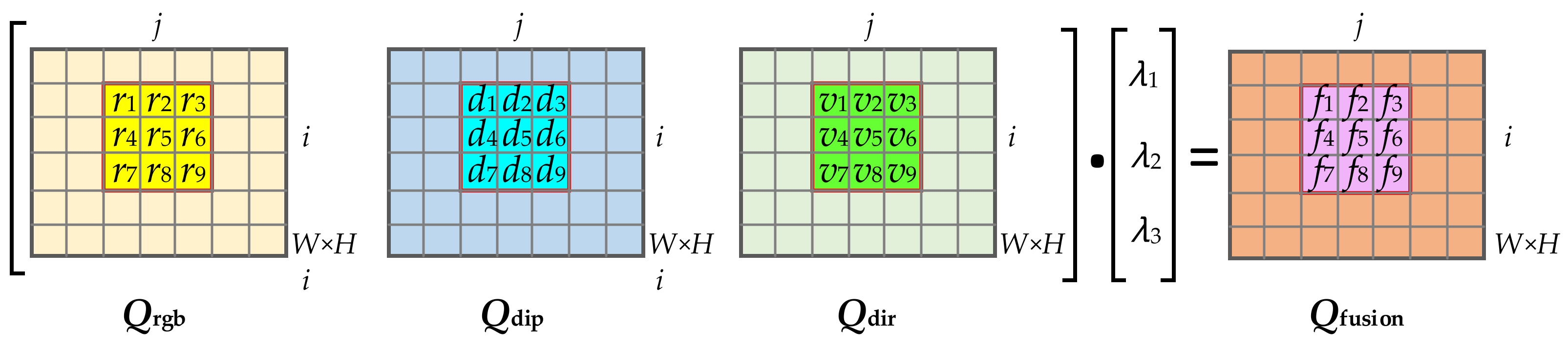
The detailed calculation process of the soft association map
is shown in
Figure 5. In
Figure 5,
–
,
–
, and
–
, respectively, refer to three probability distributions, which reflect the similarities in the RGB, dip, and dip direction semantics between the pixel
in the
i-th row and
j-th column and its surrounding nine neighboring semantic blocks.
–
represents the probability distribution of the pixel
on multi-feature semantics. The initial semantic block centers are defined by regular pixel blocks, and the centers will be optimized according to the association between each pixel and its surrounding pixel blocks. The optimization is achieved iteratively [
34]. Label mapping can be obtained by taking the maximum values of nine probabilities for each pixel, which corresponds to the result of the semantic block segmentation.
2.4. Semantic Block Clustering and Structural Plane Extraction
The semantic blocks generated from
Section 2.3 are over-segmented results, which should be further clustered to obtain the extraction results of the rock slope’s structural planes. In this study, the topological adjacency of all semantic blocks is firstly expressed by a RAG proposed by [
37]. Then, the multi-dimensional geological semantics are used to define a region dissimilarity, which measures the similarity of adjacent semantic blocks in the RAG. The RAG is further transformed into an NNG, where efficient and fast clustering of semantic blocks is achieved by merging connected bidirectional edges.
Figure 6a–d, respectively, shows the schematic diagram of the segmented semantic blocks, the corresponding RAG and NNG, and the merging results.
Figure 6a shows a superimposed display of segmented semantic blocks (blue and red curves) and an image. The numbers ①–㉔ in
Figure 6b,c represent nodes of RAG and NNG, respectively. Each node denotes a semantic block, and two adjacent semantic blocks connect with an edge, the length of which reflects the similarity of the two semantic blocks. In
Figure 6d, the blue and pink regions represent two structural planes. The semantic blocks belonging to the two regions should be merged, respectively, and then the structural planes can be extracted.
Semantic blocks are comprised of valid and invalid structural planes, and the latter may include vegetation and non-structural plane rock masses. Therefore, it is necessary to perform a further filtering process on the merging results to eliminate these invalid structural planes. For example, the RGB semantic can be used to identify green vegetation areas, and the roughness semantic can be used to recognize non-structural planes. Finally, the structural planes can be extracted successfully.
3. Experiment and Analysis
In this study, the slope of a dismissed quarry in Australia was used for the experiments. The multi-view image sequence was collected by DJI UAV. The primary optical axes of the images were perpendicular to the rock slope surface. A total of 98 digital images of the rock slope were acquired, which have enough overlap (more than 80%) to guarantee multi-view stereo reconstruction. The camera model was an FC300X, and the image resolution was 2000 × 1500 pixels. The focal length
f and ISO were set to 2.8 and 100, respectively. A total of 18 coded and 13 natural features were used as control points, and their coordinates were measured using two Leica TS11 reflectorless total stations. Therefore, the dense point cloud generated by multi-view images could be scaled. A laser scanning point cloud was acquired using a Leica ScanStation C10 TLS, and the accuracy was in the range of ±4 mm. It was used to provide the ground truth for a comparison of the geological occurrence extracted by the proposed method. The width and height of the whole rock wall was, respectively, 80 m and 6 m.
Figure 7 shows two parts of the study area of the slope, which were used for our experiments. The considered area of the wall was about 20 m long and 5 m high.
A sparse reconstruction was performed using Agisoft Photoscan software. First, feature extraction and matching were performed on multi-view images, and the essential matrix was calculated via bundle adjustment. Therefore, both interior and exterior orientation elements of the camera were estimated, and a sparse point cloud was generated with a total of 28,933 points. The sparse point cloud and camera positions are shown in
Figure 8.
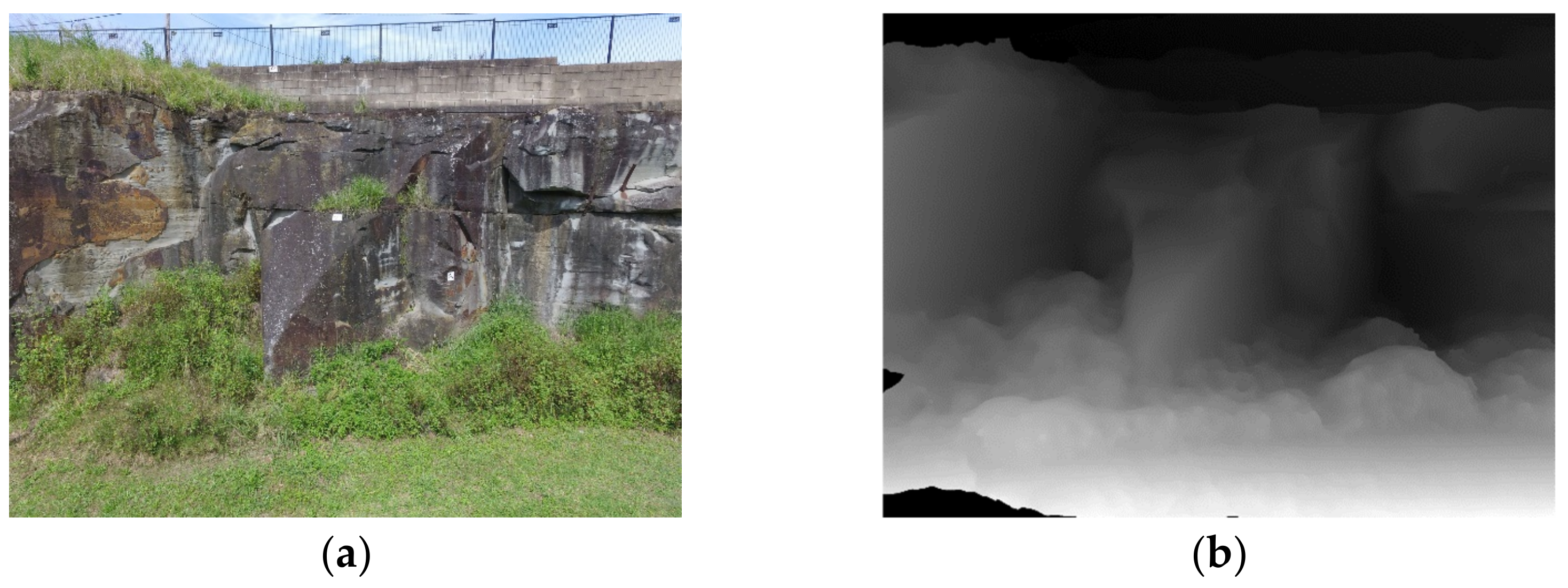
Based on the sparse reconstruction results, a PMVS dense reconstruction method was performed. A group of depth maps corresponding to the original multi-view images were generated and optimized by propagation; an example is shown in
Figure 9. The grey scale values of the depth image was in the range from 0 to 255. The values 0 and 255 represent black and white, respectively.
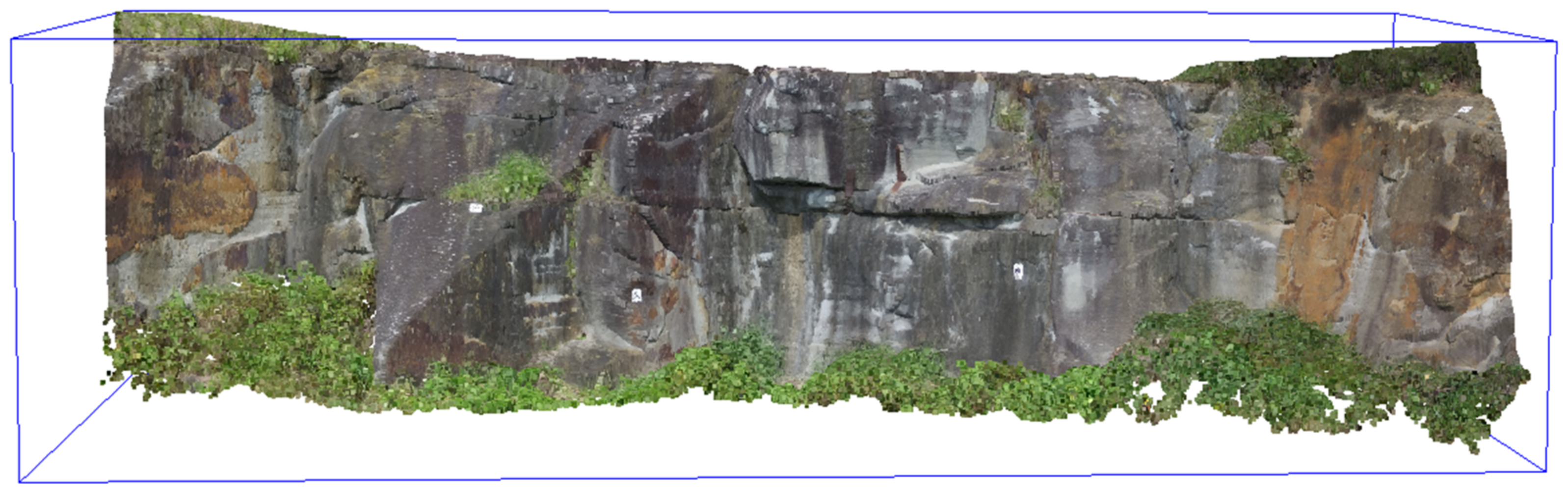
After the patch growing and expanding process, a textured dense point cloud of the rock slope was obtained. The number of points in the dense point cloud was 4,754,284; the visualization of the dense point clouds is shown in
Figure 10.
For any point in the dense point cloud, its local geological semantics involving dip, dip direction, and roughness were, respectively, calculated according to the spatial relationship between the 3D point and its surrounding local neighbor spatial points. The front view of the dense point cloud of the slope was selected for plane fitting, and then a 2D projection plane was determined. According to the projection method proposed in
Section 2.2, multiple geological semantic features were projected onto a two-dimensional plane to obtain multi-feature semantic association projection images; as shown in
Figure 11.
Figure 11a–c show projection images of RGB, dip, and dip direction semantics, respectively.
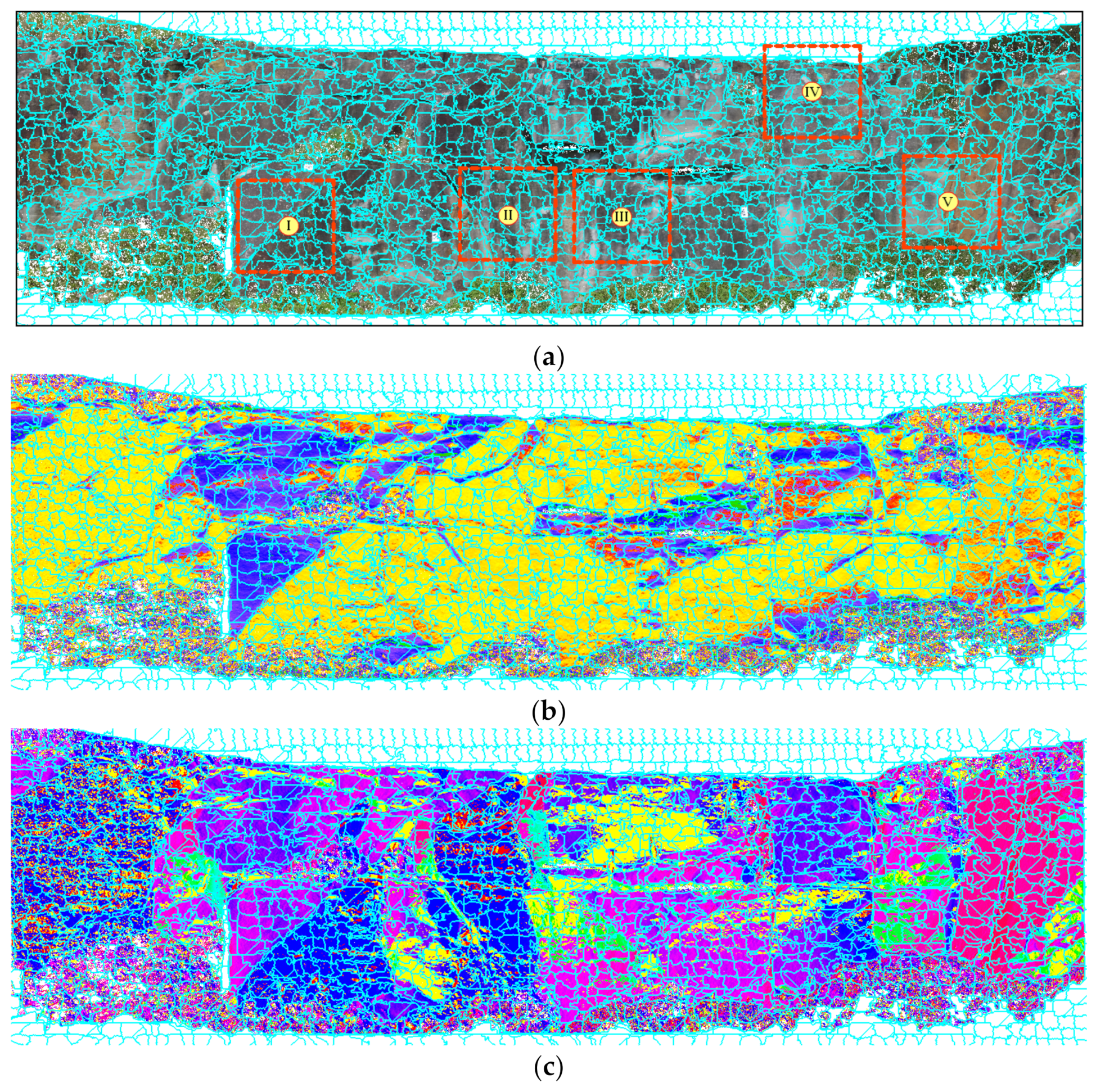
The multi-feature semantic association projection images were taken as inputs, and a semantic block set with similar geological features was generated using the Geo-AINet semantic block segmentation method proposed in
Section 2.3.
Figure 12a–c show the visualizations of the semantic block segmentation results from the proposed method on the multi-feature semantic projection images, respectively. The color range in
Figure 12b,c reflect the dip (0–90 degrees) and dip direction (0–360 degrees), respectively. The color scales correspond to
Figure 11b,c.
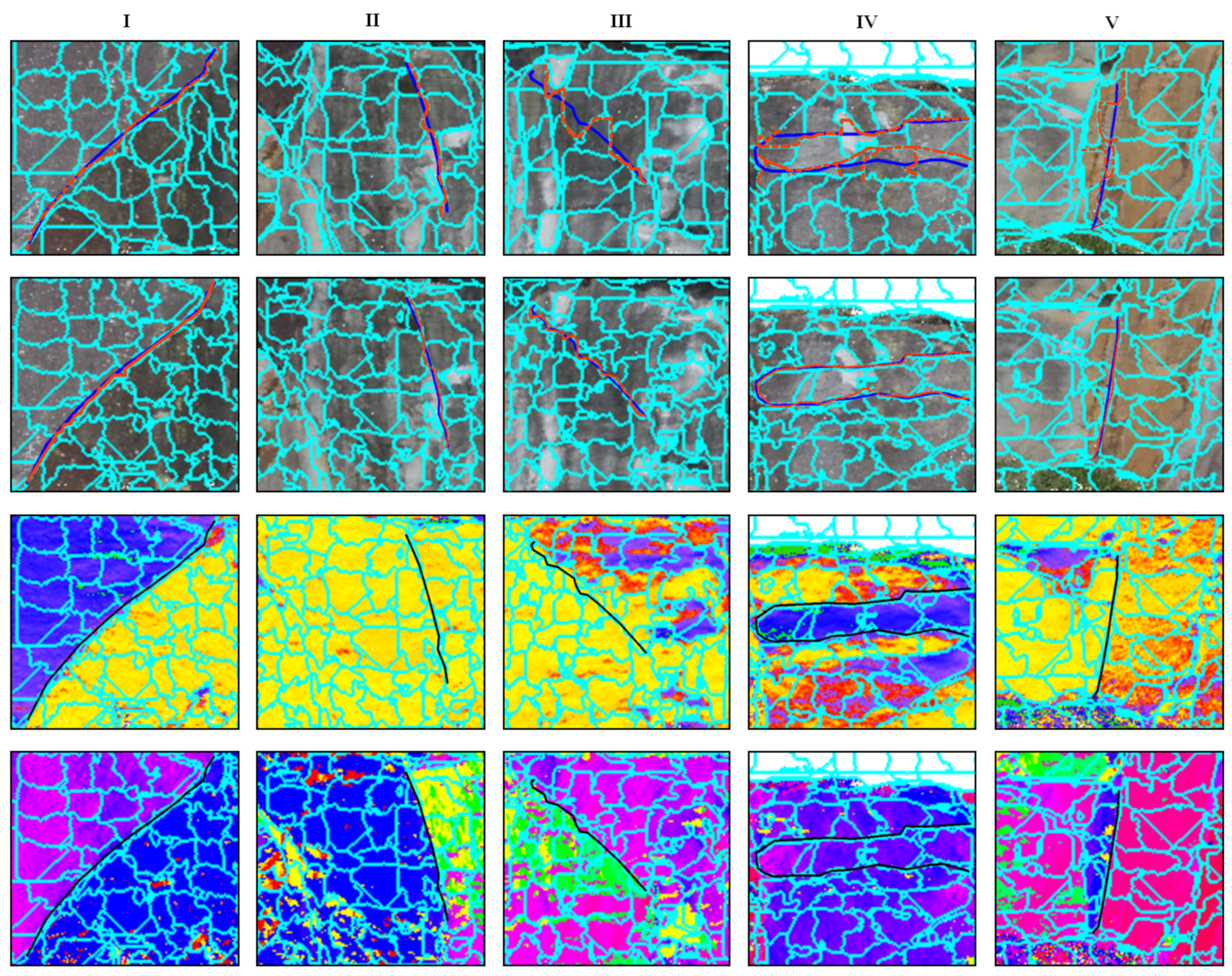
Figure 13 shows the segmentation results generated using the AINet method proposed in [
35]. The segmentation results from five regions numbered I–V (red boxes marked in
Figure 13) are compared with the corresponding results obtained by the proposed Geo-AINet method (red boxes marked in
Figure 12a).
Figure 14 shows the details of the comparison.
In
Figure 14, five examples of the local detail comparisons of the segmentation results are listed in columns. The two structural planes in region I have noticeable brightness differences caused by illumination, and both methods achieved ideal results. For region II, III, and V, the boundaries of the structural planes in the dip direction projection images are more distinctive. Similarly, for region IV, the boundaries of the structural planes in the dip projection image are easier to distinguish. In comparison with the 2D color and textures features, the 3D geological semantic features contribute to improve the segmentation accuracy of Geo-AINet. In regions II, III, and V, the structural planes have similar RGB and dip characteristics, but significantly different dip directions. It is difficult for the traditional AINet method to distinguish different structural planes accurately. Geo-AINet obtains better segmentation results because it considers the three semantics. In region IV, different structural planes can only be distinguished by the dip semantic instead of similar texture and dip direction. Therefore, the semantic blocks segmented by the Geo-AINet-based method perform better edge adherence. These experimental comparisons demonstrate, fully, that the proposed method integrates multiple geological semantics for structural plane extraction, which can effectively improve accuracy and reliability.
The semantic blocks were first merged using the clustering method described in
Section 2.4. The RAG and NNG were generated by semantic blocks with a number of 4327. Each edge connected by two adjacent semantic blocks represents a distance measurement, which was calculated by the values of the dip and the dip direction of the semantic blocks [
37]. For a semantic block, its occurrence was obtained according to the normal vector of the plane fitted by the 3D points corresponding to all the pixels in it. Therefore, the length of the edge reflects the similarity of the geological occurrence of the two semantic blocks, i.e., the smaller the distance was, the more similar the two sematic blocks. The clustering criteria is that each semantic block will be merged with the one with the closest distance to itself. Finally, those semantic blocks with the most similarity should be merged. The accuracy of the clustering results has an effect on the integrities of the extracted structural planes.
Figure 15a,b show the merging results of semantic blocks under different perspectives. In
Figure 15, the multi-feature semantic blocks have been merged successfully, and the merging results include geological structural planes and invalid surfaces, which are represented by different colors.
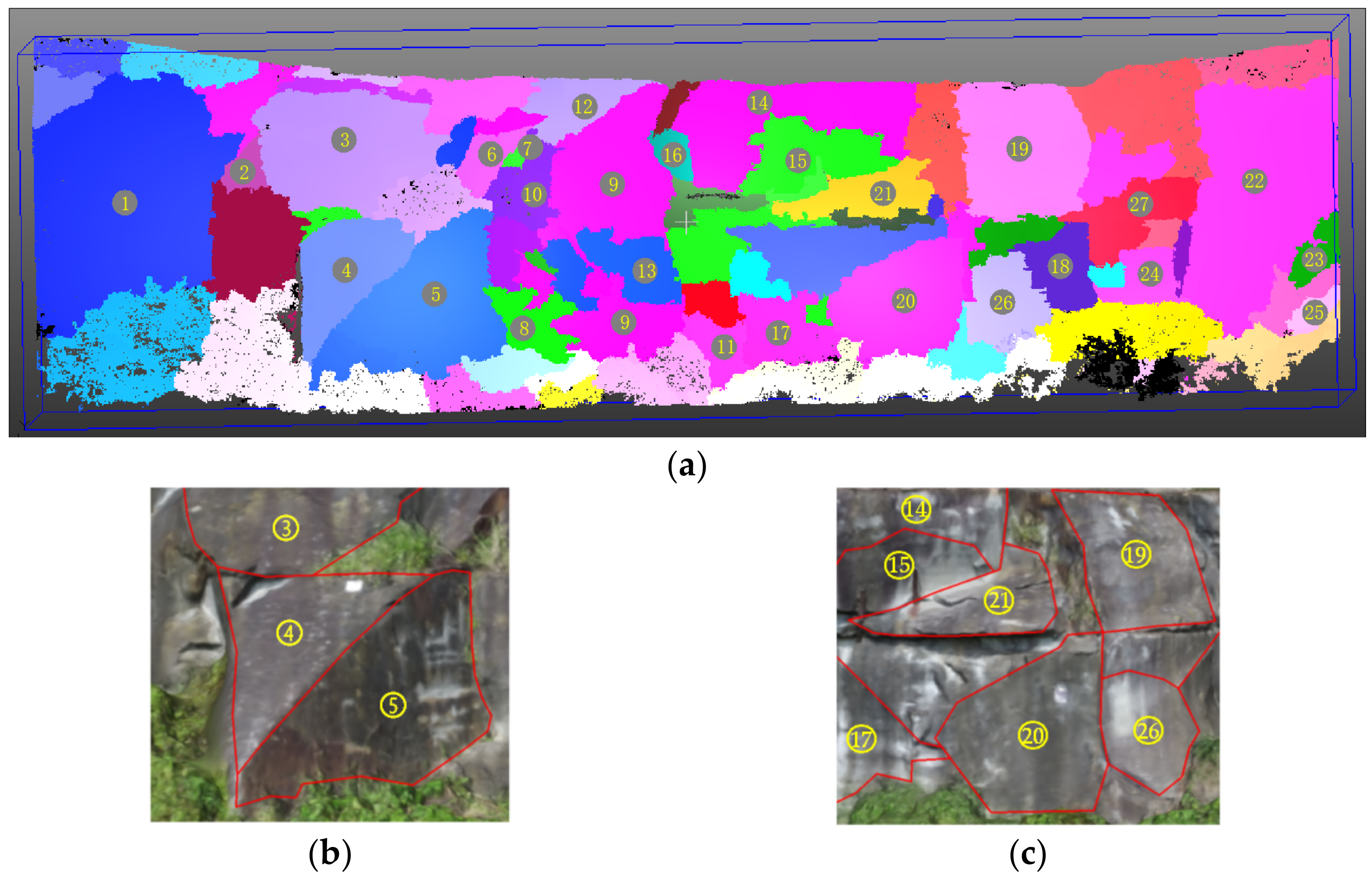
For the merging results, the color and roughness were used to filter out the vegetation and invalid structural planes regions, respectively. Finally, twenty-seven valid structural planes were successfully recognized, which are shown in
Figure 16a–c, providing a comparison of some of the structural planes displayed in the images.
4. Evaluation and Discussion
To verify the accuracy of the segmentation, four classic accuracy metrics, including Under-segmentation Error (UE), Boundary Recall (BR), Achievable Segmentation Accuracy (ASA), and Mean Distance to Edge (MDE), were used to evaluate the performance of the semantic blocks [
38,
39,
40,
41,
42]. UE represents the ratio between pixels inside the semantic block but outside the ground truth and all pixels in the ground truth. BR reflects the consistency of the boundaries of superpixels with the ground truth boundaries. A higher BR score indicates that the superpixel has better edge adherence. ASA quantifies the segmentation performance of areas that are semantic block-based instead of pixel-based, and a higher ASA score corresponds to the more accurate segmentation of semantic blocks. MDE refers to the average distance between pixels in a semantic block and the nearest boundary pixels in ground truth segmentation. The smaller the MDE score, the better the segmentation results.
The semantic block segmentation results from regions I-V, marked in
Figure 12a and
Figure 13, were used to evaluate the improvement in semantic block segmentation using the proposed Geo-AINet method versus the AINet method. The comparison results are listed in
Table 1. The under-segmentation error rate in all regions was reduced by more than 15%. The average boundary recall rate of the five regions was improved by approximately 16%, and the highest BR rate reached 85.66%. The mean distance to edge in the five regions improved vastly, roughly ranging from 19% to 37%. Compared to the other three metrics, although the achievable segmentation accuracy demonstrates a relatively moderate increase, it also reflects the superiority of the proposed Geo-AINet-based method.
Some conclusions can be obtained through the above evaluation. Since the AINet superpixel segmentation method only uses RGB for segmentation, it is difficult to accurately distinguish different structural planes with similar colors but obviously different geological occurrences. The integration of 2D and 3D geological semantic features makes the Geo-AINet method perform with apparent advantages in segmentation accuracy. For those complex geological environments, there may be various complex structural planes with obvious 2D differences in color texture and 3D geological occurrences, or a mixture of the two (some examples include the regions I–V in
Figure 14). The proposed method comprehensively considers a variety of different features, which is more conducive to the accurate extraction of these structural planes. The Geo-AINet algorithm introduces the geological occurrence semantics and integrates them with the color and roughness semantics. From
Table 1 it can be concluded that semantic block segmentation is achieved through multi-feature semantic projection and ensemble learning with Geo-AINet, which can more accurately adhere to the boundaries of complex rock mass structural planes, and performs with greater robustness. Compared with a single feature, the multiple features used for similar semantic block segmentation may improve the accuracy of structural plane extraction.
A quantitative comparison was provided to evaluate the accuracy of structural plane extraction. The dip and dip direction of the ten flat structural planes extracted by the proposed method were, respectively, calculated and compared with those correspondingly measured on the 3D laser point cloud. Firstly, an interpretation of structural planes was performed by the professional geologists according to the image and laser point cloud; then, enough laser points on the structural planes were manually selected for plane fitting; the occurrence of the structural plane was calculated according to the normal vector of the fitted plane and taken as the ground truth. It is to be mentioned that these points should be evenly distributed inside the structural surface, to try and express the spatial geometry of the structural surface. The results are listed in
Table 2. It can be seen that both the average dip difference and the average dip direction difference of the structural planes are less than three degrees, and their maximum differences are no more than four degrees. The experimental results show that the slope rock mass structural planes can be wholly and accurately identified and extracted using the proposed method. The accuracy of the results meets the relevant requirements for geology and design. Moreover, the 2D segmented results retain a mapping relationship with the 3D dense point cloud, by which the 2D results can be transmitted to the 3D structure. Deep learning can better explore the relationship between features, but it is difficult to directly perform multi-feature deep learning in 3D space due to the tremendous amount and variable dimensions of the data. Therefore, this study conducts deep learning by projecting various features into 2D space, which can effectively improve the efficiency and feasibility of the algorithm.


 ,
, 


