Article

Urban Built Environment Assessment Based on Scene Understanding of High-Resolution Remote Sensing Imagery

School of Geosciences and Info-Physics, Central South University, Changsha 410083, China
*
Author to whom correspondence should be addressed.
Remote Sens. 2023, 15(5), 1436; https://doi.org/10.3390/rs15051436
Submission received: 26 December 2022 / Revised: 27 February 2023 / Accepted: 1 March 2023 / Published: 3 March 2023
(This article belongs to the Special Issue Geospatial Big Data and AI/Deep Learning for the Sustainable Planet)

Abstract

:
A high-quality built environment is important for human health and well-being. Assessing the quality of the urban built environment can provide planners and managers with decision-making for urban renewal to improve resident satisfaction. Many studies evaluate the built environment from the perspective of street scenes, but it is difficult for street-view data to cover every area of the built environment and its update frequency is low, which cannot meet the requirement of built-environment assessment under rapid urban development. Earth-observation data have the advantages of wide coverage, high update frequency, and good availability. This paper proposes an intelligent evaluation method for urban built environments based on scene understanding of high-resolution remote-sensing images. It contributes not only the assessment criteria for the built environment in remote-sensing images from the perspective of visual cognition but also an image-caption dataset applicable to urban-built-environment assessment. The results show that the proposed deep-learning-driven method can provide a feasible paradigm for representing high-resolution remote-sensing image scenes and large-scale urban-built-area assessment.

1. Introduction

The linkage between urban built environment and life quality has attracted a lot of attention in recent years. Many studies have focused on ways to establish high-quality communities through the design of built environment that can significantly benefit public health and well-being [1,2,3,4]. Marans and Stimson described how to measure and assess the connection between the urban setting and life quality [5]. Kent and Thompson pointed out that the built environment can improve health and well-being in three ways: physical exercise, community social cohesion, and fair access to wholesome food [6]. Pfeiffer and Cloutier believed the key elements of community well-being are open, green, and natural spaces and urban layouts that promote safety and social contact [7]. Wang and Wang summarized theoretical and empirical data on how geography affects subjective well-being [8]. Mouratidis found that the built environment at community size has an impact on subjective well-being in four different ways, including social connections, leisure, physical health, and emotional experiences [9]. The impact of urban design on the quality of the built environment has been validated on many topics, such as human health [10], pedestrian activity [11,12,13,14,15], and travel behavior [15,16].
Several studies have examined how citizens perceive the built environment visually or acoustically through surveys, in-person interviews, and on-site inspections [17]. The most popular methods for conducting surveys, which capture amorphous perceptions of the built environment, are questionnaires and interviews. To measure respondents’ subjective assessment of the survey area, researchers often construct numerical-rating scales and open-ended questions. However, there have been persistent issues of response bias associated with these two approaches [18,19]. The main way to describe human impressions or emotional responses about urban design at various scales is face-to-face interviews [20]. However, due to face-to-face interviews being expensive and time-consuming, most scholars engaged in urban studies choose to conduct small-scale empirical studies [18,21].
Freely available, high-spatial-resolution crowdsourced map-service data and geotagged images have become increasingly important data sources. For example, Google Street View (GSV) can provide a panoramic view of streets and neighborhoods. Several GSV-related studies have been presented for the assessment of visual perception of urban streetscapes [18,21]. Thanks to the combination of a large amount of street-image data and deep-learning algorithms, means of analyzing the perception and understanding of urban landscapes has emerged and attracted much attention. Due to the outstanding performance in urban-street-view classification and mapping, these approaches play an important role in automatic semantic-information extraction, visual-element classification, and scene-feature representation [22,23,24,25,26,27,28,29]. However, because the street view is captured along the road, the assessment of the environment is confined to the region along both sides of the road, which is not effective for assessing the internal-area environment of the block area. Therefore, it is difficult to implement a full-coverage, continuous measurement of the built urban environment with this assessment means. Fortunately, the large coverage capability of high-resolution remote-sensing imagery allows it to objectively monitor the urban built environment from a top-down perspective. Moreover, remote-sensing images have a shorter observation period and faster update frequency, making them better able to adapt to the changing urban built environment. Due to these benefits, remote-sensing imagery has long been an important data source for urban land use/cover mapping [30,31], but its potential for assessing the urban built environment has not been fully realized mainly because the rich detailed information in high-resolution remote-sensing imagery has not been fully exploited.
The use of quantitative indicators and the calculation of indicator weights have become the main content of urban-built-environment assessment studies. These indicators come from social statistics, surveys, Street View, and GIS data; however, these data are updated less frequently and are not easily available [32,33,34,35,36,37,38]. Therefore, rather than emphasizing the selection and weighting of quantitative indicators, this study focuses on the development of an evaluation method based on the visual semantics of remote-sensing images of the urban built environment. The basic unit of urban built environment in our study is a remote-sensing-image scene within a spatial extent. Firstly, evaluation criteria are established according to their visibility in remote-sensing images and the role of different geo-objects in the environment. Secondly, the image-caption algorithm is used to explore the semantics and relationships of geo-objects in the scene image to obtain a visual semantic description of the urban built environment. Then, based on the environmental evaluation criteria, the environmental-evaluation score of the scene unit is determined according to the visual semantic description of the image. Finally, the inverse-distance weighted-interpolation algorithm is used to carry out an urban built environment.
The main contributions of this paper are as follows: (1) According to the characteristics of high-resolution remote-sensing images, the representative indicators of the urban-built-environment criteria of geographic scenes are established. (2) A natural-language dataset for urban-built-environment evaluation is established. (3) The image-caption model is employed to evaluate the urban built environment for the first time.
The remainder of this paper is organized as follows. Section 2 introduces the methodology, including the constructed-scene-assessment criteria, dataset, and assessment model. Section 3 presents the experimental results and analysis. Section 4 discusses and explores the applicability of this research method in different cities and mentions the strengths and limitations of the proposed method. Section 5 concludes with some remarks and potential future research directions.

2. Methodology

2.1. Overview

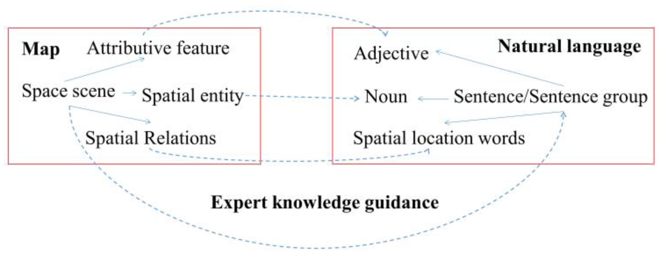
Vision is the main form of human perception, and language is the most powerful tool for human communication with the world [39]. Humans can utilize language to transmit information according to their perception of the geographical environment [40]. This study intends to carry out an environmental assessment from the perspective of spatial understanding of remote-sensing-image scenes. The image-caption model is used to create language descriptions of geographic scenes. The general framework of the proposed methodology is shown in Figure 1. Firstly, it establishes criteria for assessing the urban built environment from remote-sensing images from the perspective of human visual perception. Secondly, we construct an image-caption dataset of the built environment based on the assessment criteria and utilize the dataset to train an image-caption model to support the assessment. Finally, the image-caption model and the assessment criteria are jointly utilized to assess the built environment of Changsha.

2.2. Assessment Criteria

The visual elements in the built-environment scene play a fundamental role in evaluating the built environment from a visual-perception perspective, as shown in Figure 2. Therefore, considering the visibility of distinct urban visual elements in high-resolution remote-sensing images, the following five assessment indicators were established. The specific description of each indicator is given below.
Building density. As the urban population increases, the impact of building on the assessment of the urban built environment is increasingly worth considering. Density is the most immediate and representative factor of the urban built environment [41]. The space between buildings is important for comfortable outdoor time [42]. Studies have shown that building density is directly correlated with community satisfaction [43,44]. Low-density settlements are appreciated for their spacious living environment [45]. High building density can also lead to the heat-island effect, which reduces the wind speed among buildings and increases the ambient temperature [46]. This paper refers to the criteria of Stewart and Oke [47], namely, based on whether the density is greater than 40%, the building area is divided into an open-building area and a compact-building area. In this criteria, open buildings were positively correlated with the assessment results, whereas dense buildings were negatively correlated with the assessment results.
Road connectivity. Roads are not only places for the transportation activities of residents in residential areas but also used as spaces for social interaction, which has an important influence on environmental quality. Wei et al. [48] and Duan et al. [49] identified road connectivity as one of the factors that determine the walkability of a neighborhood. Malambo et al. [50] also showed that urban attributes such as road connectivity improve the walkability of the community, thereby promoting the development of physical activities such as walking and recreation, which can help reduce the incidence of disease. Xu et al. [51] mentioned that road connectivity has an effect on community vitality. In this paper, good and bad connectivity is distinguished by the road structure in the geographic scene. The road structure of the geographic scene is a grid structure or a tree structure. The grid structure has a homogeneous distribution, is usually straight, and has good connectivity; on the contrary, the tree-structured road network is dendritic, mainly in some old communities, and has poor connectivity [52].
Vegetation coverage. Vegetation coverage has always been an important indicator of the quality of the living environment and plays a very important ecological role in residential areas, such as oxygen release, cooling, humidity control, shading, wind protection, dust blocking, sun protection, noise reduction, acting as an insecticide, and other functions [51]. Urban vegetation cover is one of the reasons for comfort, improves air quality, reduces the effects of noise pollution and extreme weather events, and promotes mental health by reducing stress [53]. Hur et al. [44] found that vegetation is an important factor in space use, security and adaptability, and informal social contact between neighbors. Numerous studies [54,55,56,57] have shown that the vegetation cover in residential areas often leads to positive evaluations of the environment. Therefore, the presence of vegetation cover around buildings is positively correlated with the assessment results.
Distribution of industrial areas. With the development of industry, residential areas and industrial areas coexist in large cities, and sometimes the distance between industrial areas and residential areas is less than 100 m [55]. However, industrial areas have a negative impact on the surrounding area and affect the aesthetic quality of the environment [58]. People are less likely to engage in recreational activities near industrial areas [59]. Existing studies [58,60] have shown that the presence of an industrial area often leads to a negative assessment of the environment. Therefore, the presence of industrial areas is negatively correlated with the evaluation results.
Distribution of activity areas. Open activity can enhance human comfort. Research [60] has shown that open, green spaces have a positive impact on the quality of urban life. Douglas et al. [61] surveyed 483 residents living in three communities in Dublin, Ireland, and found that open, green spaces are important predictors of high community satisfaction. The presence of neighborhood green spaces, such as parks and woodlands, is associated with better physical health, lower rates of certain categories of disease, and lower levels of depression. In addition, the study by Ambrey and Fleming [62] showed that a neighborhood surrounded by water is an exciting place to live. Malambo et al. [50] found that the presence of sports and recreational facilities can increase the physical activity of residents. Therefore, the presence of an activity area often leads to people’s positive assessment of the environment. In this paper, rivers, lakes, green spaces, and playgrounds, which are common factors of urban-life satisfaction, were selected as activity-space elements. In our defined criteria, the presence of these activity areas was positively correlated with the evaluation results.
In this paper, 0 and 1 represent the evaluation results for each evaluation metric. The score was set to 1 and 0 for positively correlated results and negatively correlated results, respectively.
After clarifying the performance of each indicator, the final evaluation score was obtained by summing the scores of each indicator. The image-caption model was used in this paper to mine remote-sensing-scene information. Commonly used weight-setting methods such as AHP [63] and principal-component analysis [64] were not suitable for this paper. In our method, the indicators were expressed in natural language, and the quantitative results of each indicator were not calculated, so the traditional weight-setting method was not applicable. Therefore, after comprehensive consideration, the total score was obtained by adding each indicator to show the comprehensive performance of each indicator. This method can more easily correspond to the content of natural-language description and provide the most direct understanding of the assessment results of urban scenes, which can be calculated as follows:
X = i = 1 5 x i ,
where X represents the total score of the evaluation results, reflecting the comprehensive performance results of the five indicators; and xi represents the score of each indicator and takes a value of 0 or 1. Based on the above, the assessment criteria were determined, as shown in Table 1.

2.3. Dataset and Model

2.3.1. Dataset Establishment

A large number of studies have used image-caption models for spatial understanding of remote-sensing-image scenes in recent years [65,66,67,68,69]. Given a high-resolution remote-sensing image, the computer mines the visual-feature information of the image and expresses the information in the form of natural language. The automatic generation of an image-content description that matches human cognition and expression habits has become a new way to transfer remote-sensing-image information.
Existing image-caption datasets mainly include the UCM-caption dataset [67], Sydney-caption dataset [67], and GRIUD dataset [65]. The UCM-caption and Sydney-caption dataset simply describe the objects in the image, with labels such as “there are two planes on the airfield”, and “this is a beach”. It is only suitable for spatial cognition of simple geographic scenes. The GRIUD dataset proposes a semantic understanding of remote-sensing images from the perspective of geospatial relationships. Although this dataset can mine richer spatial information, it cannot achieve the goal of environmental assessment.
The existing image-caption datasets are limited to expressing the objects and their relationships and cannot meet the requirements of this paper. Therefore, based on the above assessment criteria for spatial understanding of remote-sensing-image scenes, this work deeply explores the composition of remote-sensing scenes, determines the relevant vocabulary and grammatical structure, and establishes a dataset dedicated to this study.
With the improvement of earth-observation capabilities, massive high-resolution remote-sensing-image data can provide large-scale, rich, and updated ground information. In this paper, high-resolution remote-sensing images of the central urban area of Changsha were selected to build a dataset. The high-resolution remote-sensing images were collected from Google Earth with a spatial resolution of 0.5 m, containing three visible bands of red, green, and blue. To meet the input requirements of the image-caption model, this paper cropped these images to obtain image patches, and each image patch corresponds to a geographic-scene unit containing different geographic elements.
Cropping at different scales results in geographic-scene cells of different spatial extents. If the spatial extent of the scene was too small (Figure 3a), the geographic elements were uniform and could not reflect the surrounding environmental information, resulting in very small differences between such scene units. Conversely, if the spatial extent of the scene was too large (Figure 3c), it was difficult to focus on the local spatial environment because it contained many geographic elements. In order to determine the appropriate scene-unit size, this study carried out scene-unit division with different scale sizes and finally decided to use an image block with a size of 250 × 250 as the basic unit. The scene unit of this scale can include a reasonable number of geographic elements and information about the surroundings, thus facilitating the urban-built-environment assessment in this study. After cropping the remote-sensing image of the main urban area of Changsha, we obtained a total of 3874 images with a size of 250 × 250.
Since this work analyzed the environmental assessment of urban scenes based on remote-sensing images, further filtering of the cropped images was required after obtaining remote-sensing scenes. The principle of filtering is to delete the images that did not contain any building areas and the images that contained architectural areas but did not belong to urban areas. For example, due to the main elements in Figure 4a being water bodies and Figure 4b showing that its main elements are water bodies and forests, both of these images should be filtered out accordingly. In addition, Figure 4c contains many buildings but is located in a rural area; thus, it also does not meet the requirement. Finally, 836 images of these types were discarded.
Next, the remaining 3038 remote-sensing-scene images needed to be labeled to establish the Environmental Assessment Dataset. To this end, 10 senior GIS students were invited as volunteers to manually describe and assign scores to each image. The newly recruited volunteers were trained in two steps. The first step was sketch construction, which focused on identifying geo-objects and their spatial relationships. The second step was sentence expression, which mainly included elimination of irrelevant geo-objects and natural-language description. After the training, all of the volunteers were assigned to practice describing the same images many times until they could achieve the same perception in most cases.
Sketch construction: Spatial relationships can represent the interdependent distribution of geo-objects in the spatial environment and are the key content of spatial understanding in geographic scenes. In this study, we referred to the spatial-relationship expression in [65], which provides a technical basis for generating descriptions of various topics. The sketch construction involves both identifying geographic entities in a scene and extracting sketches based on the spatial relationships among these entities, as shown in Figure 5.
Sentence description. After sketch construction, irrelevant geo-objects such as parking lots and golf courses were eliminated from the sketch and then the simple geographic relationship of the sketch was expressed as a natural-language description. Geographic-scene description is a collection of geographic entities, spatial relations, and attributes. This paper referred to the description rules in [65] and converted the sketches into natural-language descriptions containing geographic knowledge. For example, we used nouns to represent spatial entities, such as “building area”, “industrial area”, “trees”, “roads”, “playgrounds”, “rivers”, and “lakes”. Spatial relationships were represented by prepositions, such as “around”, “near”, and “adjacent”. Adjectives were used to describe the characteristics or attributes of geographic entities; e.g., “open” and “compact” were used to characterize the properties of building density (Figure 6).

2.3.2. Image Caption

In this study, the image-caption model was adopted to provide a potential way to mine geographic knowledge in remote-sensing images and provide strong support for understanding scenes. Despite many studies having developed remote-sensing image-caption models [65,66,67,68,69], these models only output one sentence to describe the whole image. This study conducted built-environment assessment based on remote-sensing-image scenes from five perspectives, i.e., it aimed to generate sentences on five different topics by using image caption. Thus, to enable adaptation of the task, a multi-task hierarchical model [70] was improved in this study to automatically generate descriptions of five different topics from remote-sensing images (Figure 7).
Given a high-resolution remote-sensing image, a CNN model was used to learn the visual features { v n } n = 1 N D . The visual features were then fed into a multi-label classification network (MLC) to predict the tag labels:
p l , p r e d ( l i = 1 | { v n } n = 1 N ) exp ( MLC i ( { v n } n = 1 N ) ) ,
where l L is a label vector, li = 1/0 represents the presence and absence of the ith label, and MLCi represents the ith output of the MLC network. The obtained result was used to output the semantic features on five different topics, where the semantic features { a m } m = 1 M E are the embedding-vector representations of the labels.
Then, the visual features { v n } n = 1 N D and semantic features { a m } m = 1 M E were fed into an attention-mechanism model to generate a context vector c t x ( s ) C . The attention model employed a single-layer feed-forward network to compute visual and semantic attention on input image features and labels.
α a , m exp ( W a a t t tan h ( W a a m + W a , h h s e n t ( s 1 ) ) ) ,
α v , n exp ( W v a t t tan h ( W v v n + W v , h h s e n t ( s 1 ) ) ) ,
where W v , W v , h , and W v a t t are the parameter matrices of the visual-attention network; W v a t t , W a , h , and W a a t t are the parameter matrices of the semantic-attention network; and h s e n t ( s 1 ) H are the hidden states of the sentence LSTM at time-step s − 1. I context vector c t x ( s ) C is calculated as follows:
v a t t ( s ) = n = 1 N α v , n v n ,     a a t t ( s ) = n = 1 N α a , m a m ,
c t x ( s ) = W f c [ v a t t ( s ) ; a a t t ( s ) ] ,
Next, starting from the context vector, decoding generated a textual description. The model produced sentences hierarchically: It first generated high-level topic vectors representing different sentences and then generated a sentence from each topic vector. Specifically, the context vector was input into a sentence LSTM, which is a single-layer LSTM. The input context vector was used to generate a sequence of hidden states h s e n t 1 , , h s e n t s H , each sentence corresponding to a hidden state, and the hidden state was used to generate a topic vector t ( s ) P for each sentence, as the input to the word LSTM.
t ( s ) = tan h ( W t , h s e n t h s e n t ( s ) + W t , c t x c t x ( s ) ) ,
where W t , h s e n t and W t , c t x are the parameter matrices, and h s e n t ( s ) is the hidden state of the sentence LSTM at the moment.
Given a topic vector t ( s ) , the word LSTM took it as input and progressively generated sentences. The initial input to the word LSTM was the topic vector and an embedding vector W e s 0 of the START input indices s 0 , and the subsequent inputs were the topic vector and the embedding vector W e s 1 , , W e s N 1 of true word labels s 1 , , s N 1 . At each time step, the word LSTM hidden state h w o r d 1 , , h w o r d N H was used to predict words p 1 , , p N . After each word LSTM generated the words of the respective sentences, the sentences were finally concatenated to form the generated paragraphs.
x t = W e s t ,
h w o r d t + 1 = LSTM ( t ( s ) , x t , h w o r d t ) ,
p t + 1 e x p ( W o u t h w o r d t + 1 ) ,
where W o u t is the parameter matrix, and h w o r d is the hidden state of the word LSTM.
The model used MLC to perform multilabel classification on images, encoding the presence and absence of labels. The training loss for this step was the cross-entropy loss L t a g between the multiclass predicted values and the true labels. Next, the topic vector S was generated on the sentence LSTM, and then, the five generated topic vectors were input into the word LSTM step by step to generate words. The training loss for this step was the cross-entropy loss L w o r d between the generated word pt and the ground-truth label st. Therefore, the overall training loss was as follows:
L ( I , l , w ) = λ t a g L t a g + λ w o r d L w o r d ,
where λ t a g and λ w o r d correspond to the weights of the multilabel-classification loss Ltag and the sentence-output loss Lword, respectively. The overall training procedure is summarized in Algorithm 1.
Algorithm 1: Training Image-Caption Model
1.
Input: Dataset D = { x n = ( I n , l n , w n ) , n = 1 N } ; // I n is a remote sensing image, w n are the ground-truth sentences. l n denotes the ground-truth tag vector, which is extracted from w n .
2.
Output: f C N N ( · ) , f C O a t t ( · ) ,   f M L C ( · ) , f s e n t L S T M ( · ) ,   f w o r d L S T M ( · ) ;     / /     f C N N ( · ) , f C O a t t ( · ) ,   f M L C ( · ) , f s e n t L S T M ( · ) ,   f w o r d L S T M ( · ) respectively represent the weight parameters of the CNN module, co-attention module, MLC module, sentence LSTM, and word LSTM.
3.
Hyperparameter: λ t a g ,   λ w o r d ;
4.
For each epoch:
5.
 Extract image features v n f C N N ( I n ) ;
6.
 Predict the tag labels p l e x p ( f M L C ( v n ) ) ; / /Equation (2).
7.
 Embed semantic features a m p l . p r e d ; / / a m are the embedding vectors of the labels.
8.
 Compute the context vectors c t x ( s ) f C O a t t ( v n , a m ) ; / /Equations (3)–(6).
9.
 Compute the topic vectors t ( s ) f s e n t L S T M ( c t x ( s ) ) ; / /Equation (7).
10.
 Predict the words p w o r d f w o r d L S T M ( t ( s ) ) ; / /Equations (8)–(10).
11.
 Compute the loss L λ t a g C E ( p l , l n ) + λ w o r d C E ( p w o r d , w n ) ; / / C E ( · ) is the cross-entropy
  loss function, and this step refers to Equation (11).
12.
 End.
In this study, visual features were extracted using ResNet152 in the encoding stage to obtain visual features of the size 14 × 14 × 512. The visual features were fed into the MLC to obtain the classification results, which were converted into an embedding vector of 512 dimensions. For the hierarchical LSTM, the dimension of both the sentence-LSTM and the word-LSTM hidden states was set to 512 and the size of the initial learning rate was 0.001. The model was optimized by the Adam method. The parameters λ t a g and λ w o r d were 0.5 and 2, respectively.

2.4. Environmental-Assessment Mapping

As the basic analysis unit of this paper was a remote-sensing scene of the size 250 × 250, the assessment result of the built environment may have been affected by the cropping of remote-sensing images. For example, when the spatial-grid unit is relocated to the left or right, the main elements contained in it may change. The spatial-grid unit in Figure 8a,b are spatially adjacent. Figure 8a contains an industrial area. Although the residential area in Figure 8b is quite close to this industrial area, the industrial area cannot be included in Figure 8b due to the effect of cropping. Although the proposed evaluation method can be analyzed well in a single remote-sensing scene, the assessment of the entire urban built environment must not consider individual scene units in isolation.
Therefore, this paper adopted the interpolation method after sampling to reduce the effect of cropping. At first, we increased the sampling in two steps: (1) The initial sampling spatial-grid unit was moved to the four directions of east, south, west, and north, and the moving distance was 1/2 of the range of the spatial grid unit, that is, 125 pixels. Then, we used the image-caption model to describe the moved spatial-grid unit and obtained the assessment score of each unit. (2) The spatial-grid unit was converted into a center point, which was convenient for subsequent interpolation operations. The attribute of the point was the environmental-assessment score, which was equal to the assessment score of the spatial-grid unit centered on the point. This process aimed to increase the coverage sampling of the original spatial-grid unit and reduce the effect of cropping. The method of moving the spatial-grid unit and obtaining the center point is shown in Figure 9.
Next was the interpolation of the obtained center points. In this study, the inverse distance-weighting method was used to interpolate the obtained sample points. The inverse distance-weighting method is based on the first law of geography. Therefore, the influence of a known point decreases as the distance increases, and the weight is inversely proportional to the square of the distance [71]. In this study, the maximum distance of the point search radius in the inverse distance-weighting method was set to 125. The assessment map generated by interpolation can retain the characteristics of the point itself, and it can integrate the mutual influence between the point and the surrounding points, which can reduce the influence caused by cropping to a certain extent.

3. Results

3.1. Study Area and Data

Changsha is the capital of Hunan Province. It has a large undulating terrain, diverse landform types, and developed surface-water systems. The Xiang River runs through the city from south to north. On the east bank of the river is the main urban area of Changsha City, where the density of buildings and roads is relatively high, and on the west bank of the river are some new urban areas, with low building density and large areas of vegetation cover. In this study, the central urban area of Changsha, which is distributed on both sides of the Xiang River, was selected as the study area (Figure 10). The data used in this study were the high-resolution remote-sensing images covering the central urban area of Changsha.

3.2. Implementation Details

All experiments were performed in the PyTorch framework with one NVIDIA 2080Ti GPU. The experiments were carried out using the established dataset, in which 80% and 20% of the images were used as training and test sets, respectively.

3.3. Model Performance

Table 2 shows the performance results of our trained model on the test set (615 images). The correctness of the sentence for each image in the test set was computed using the following formula:
Proportion 1 = N i N ,
where Ni represents the correct number of pictures for i sentences, the value range of i is 0–5, and N represents the total number of pictures.
Statistical analysis showed that the model accurately predicted the assessment sentences of 85.69% of the images (all five indicators were accurately predicted), 12.52% of the images had one indicator incorrectly predicted (four indicators were accurately predicted), 1.46% of the images had two indicators incorrectly predicted (the prediction of three indicators was accurate), and no prediction error of more than two indicators.
To better evaluate the model, the assessment results of the model on five different indicators are shown. For each image in the test set, the prediction accuracy was calculated using the following formula:
Proportion 2 = N j N ,
where Nj represents the number of pictures with the correct jth indicator, j corresponds to indicators of different topics, and N represents the total number of pictures.
Table 3 shows that the image-caption model achieved more than 93% prediction accuracy on the five indicators and performed well in discriminating between high and low quality for each indicator.

3.4. Assessment Results

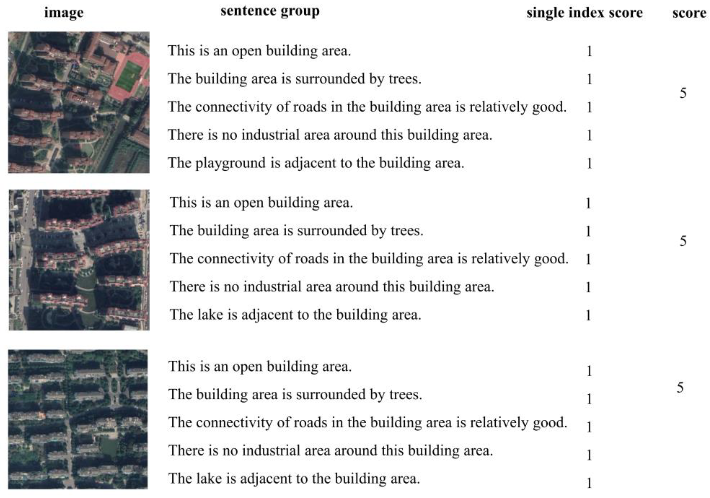
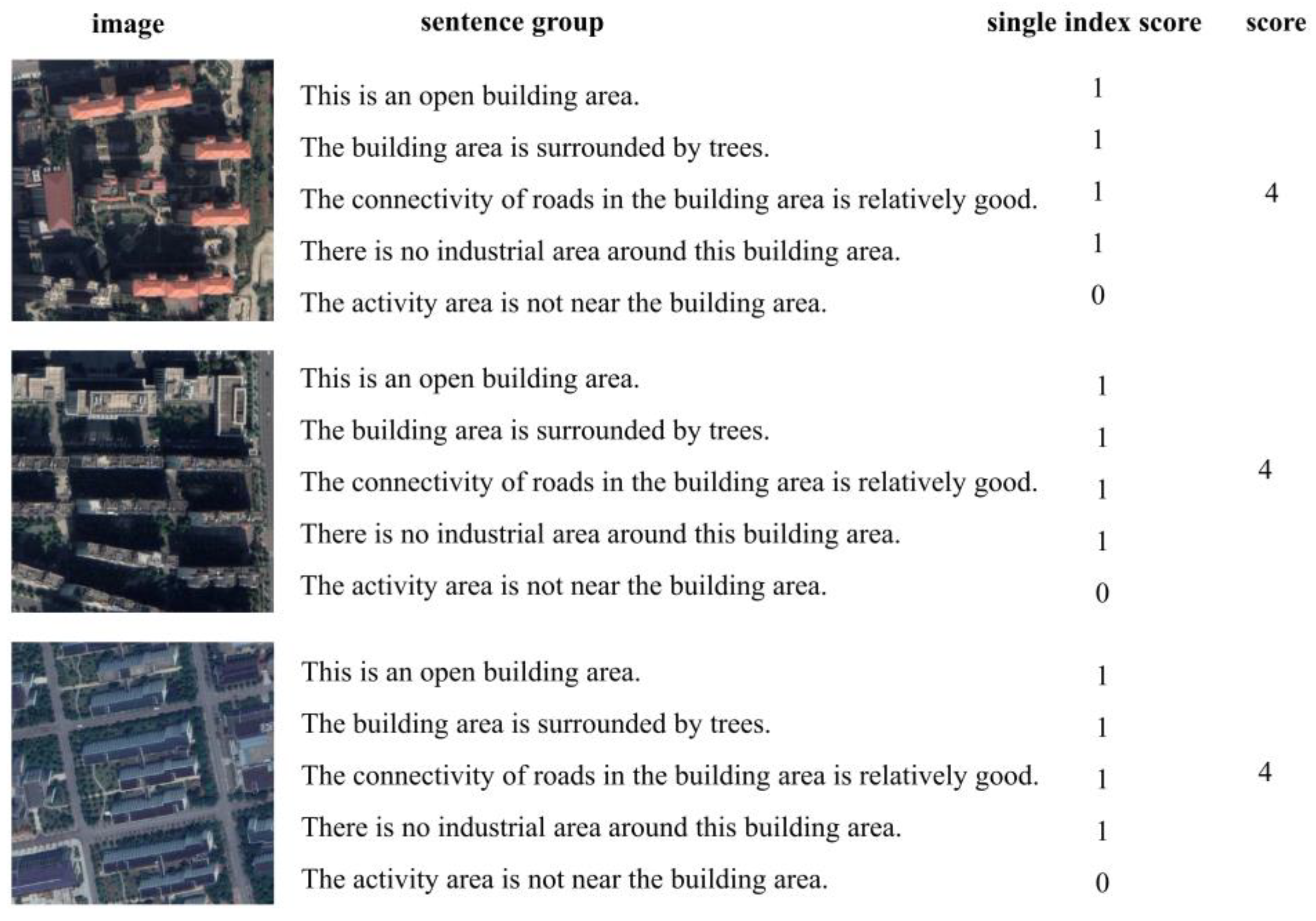
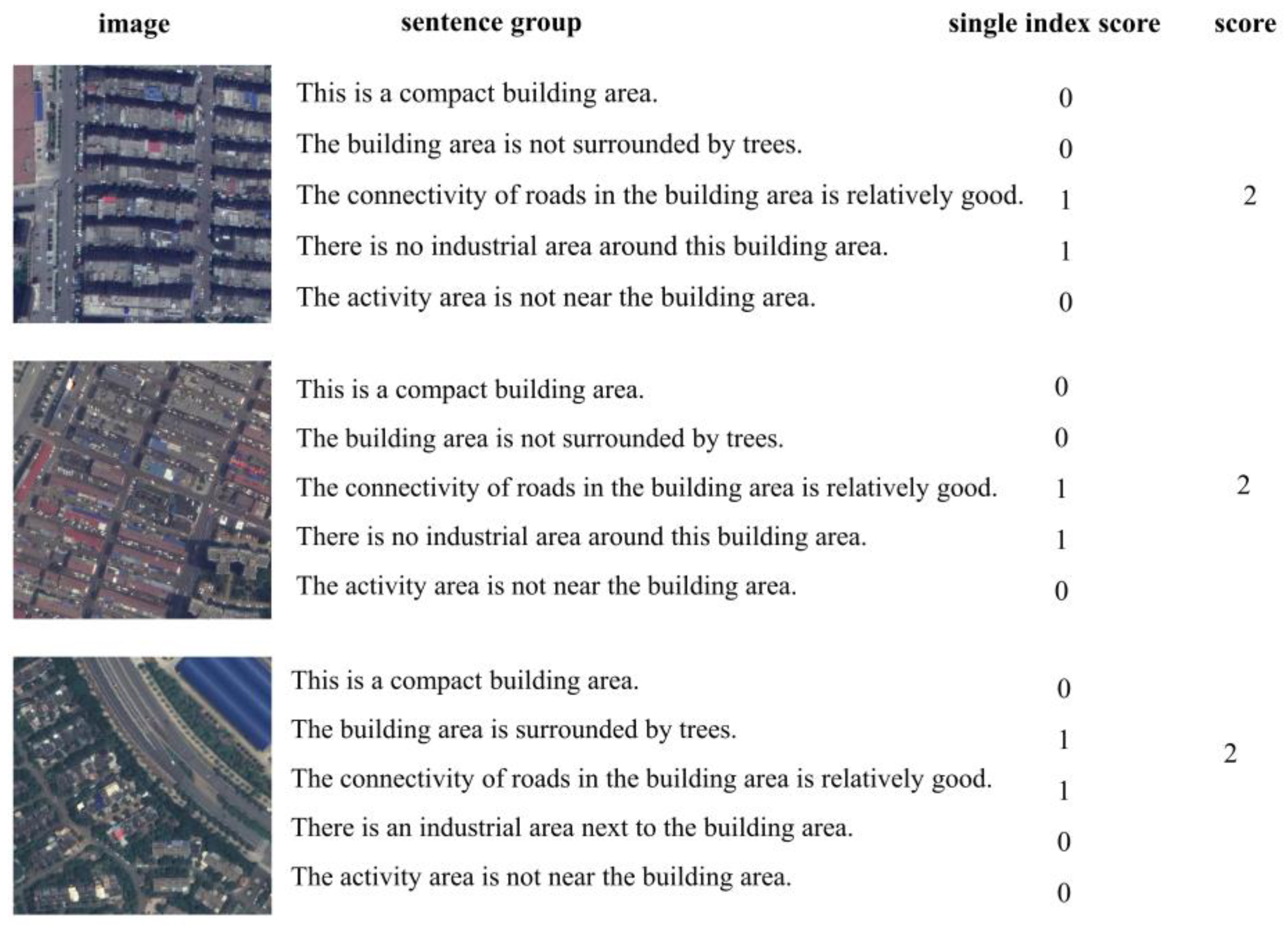
Using the image-caption model trained on the test set of the Environmental Assessment Dataset, the model generated five sentences for each remote-sensing image for description. The generated sentences were then analyzed and the built-environment scores were calculated with reference to the evaluation criteria.
This section shows the sentence results for each image patch (scene unit), although the images cannot fully reflect all the complex scenes in the city and all the performances in each score. However, through these typical images, this work found that for the scenes with the same score, their performances were similar, which may reflect some representative scene characteristics.
These results also show that our method can evaluate geographic scenes from a visual perspective and can simulate human cognition and discriminate environmental quality. (1) For scene units with scores of 5, the quality of the five evaluation indicators was relatively high, which was represented by an open-building layout, high vegetation coverage, good road connectivity, no industrial interference, and space for leisure activities. (2) For scene units with scores of 4, most of them performed well in the four indicators of building density, vegetation coverage, road connectivity, and industrial area, but it was difficult to meet the indicator of the activity area. (3) For scene units with scores of 3, the performance was relatively more diverse; some geographic scenes showed a lack of vegetation coverage but the buildings were more open, and some geographic scenes showed higher vegetation coverage but denser buildings. (4) For scene units with scores of 0, 1, and 2, the indicator of building density performed poorly and most of them lacked vegetation coverage. Among them, scenes with scores of 2 had more open-building density than scenes with scores of 0 and 1, and performed better on the road-connectivity indicator. Scenes with scores of 0 and 1 had dense and irregular buildings, poor road connectivity, and lack vegetation coverage and activity space. Scenes with scores of 0 had industrial areas. The examples in Figure 11, Figure 12, Figure 13, Figure 14, Figure 15 and Figure 16 show that the transition from the highest score to the lowest score is consistent with the results of people’s spatial cognition of geographic scenes, indicating that our method can simulate human perception. The accurate expression of natural language also demonstrates the effectiveness of our assessment method, which can fully describe the specific environmental elements in high-resolution remote sensing images through natural language. These results can fully demonstrate the representativeness of our assessment indicator. Through the organization of five different indicators, the organization of high-resolution remote-sensing-image scene elements can be fully exploited to carry out environmental assessment.

3.5. Built-Environment Assessment

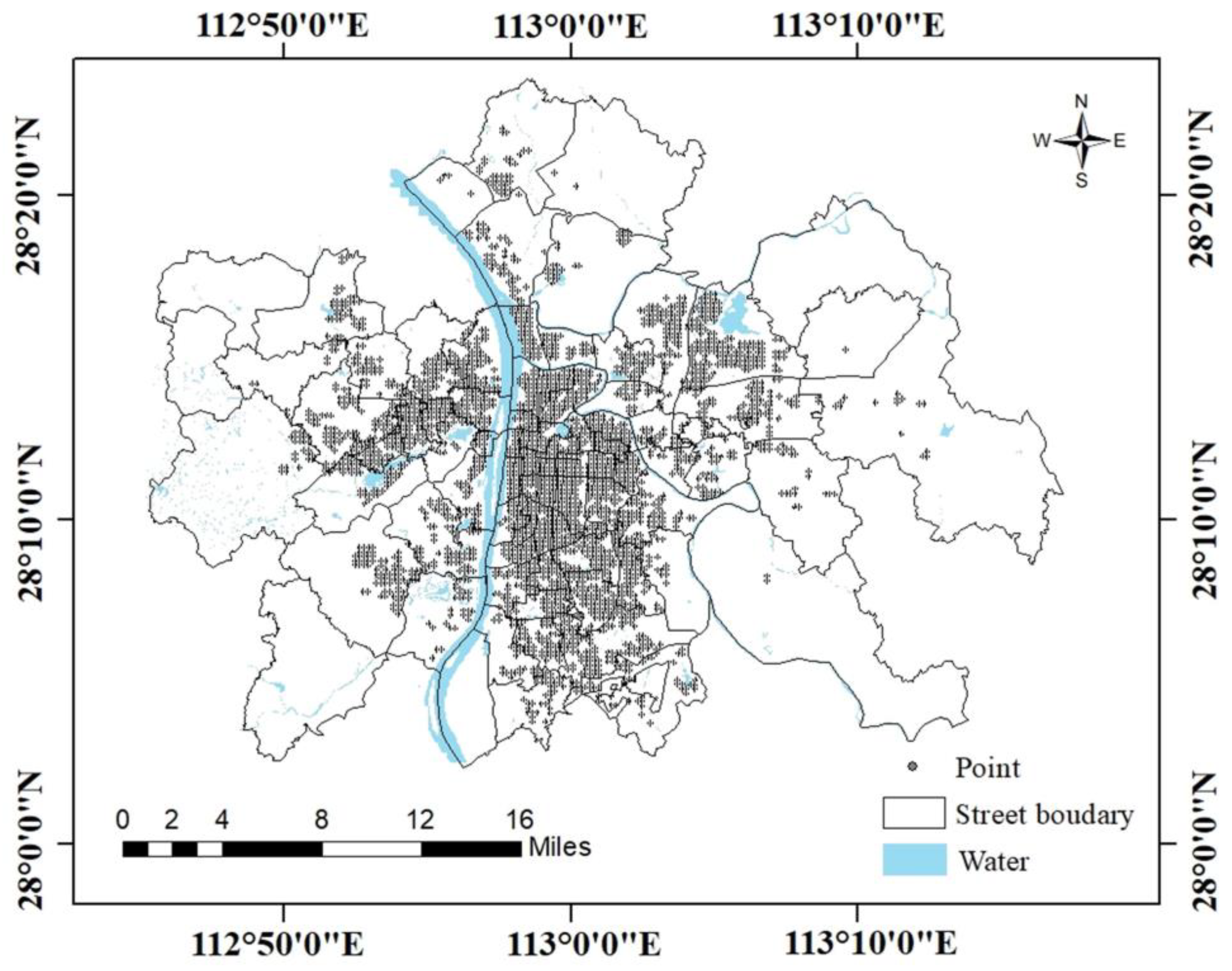
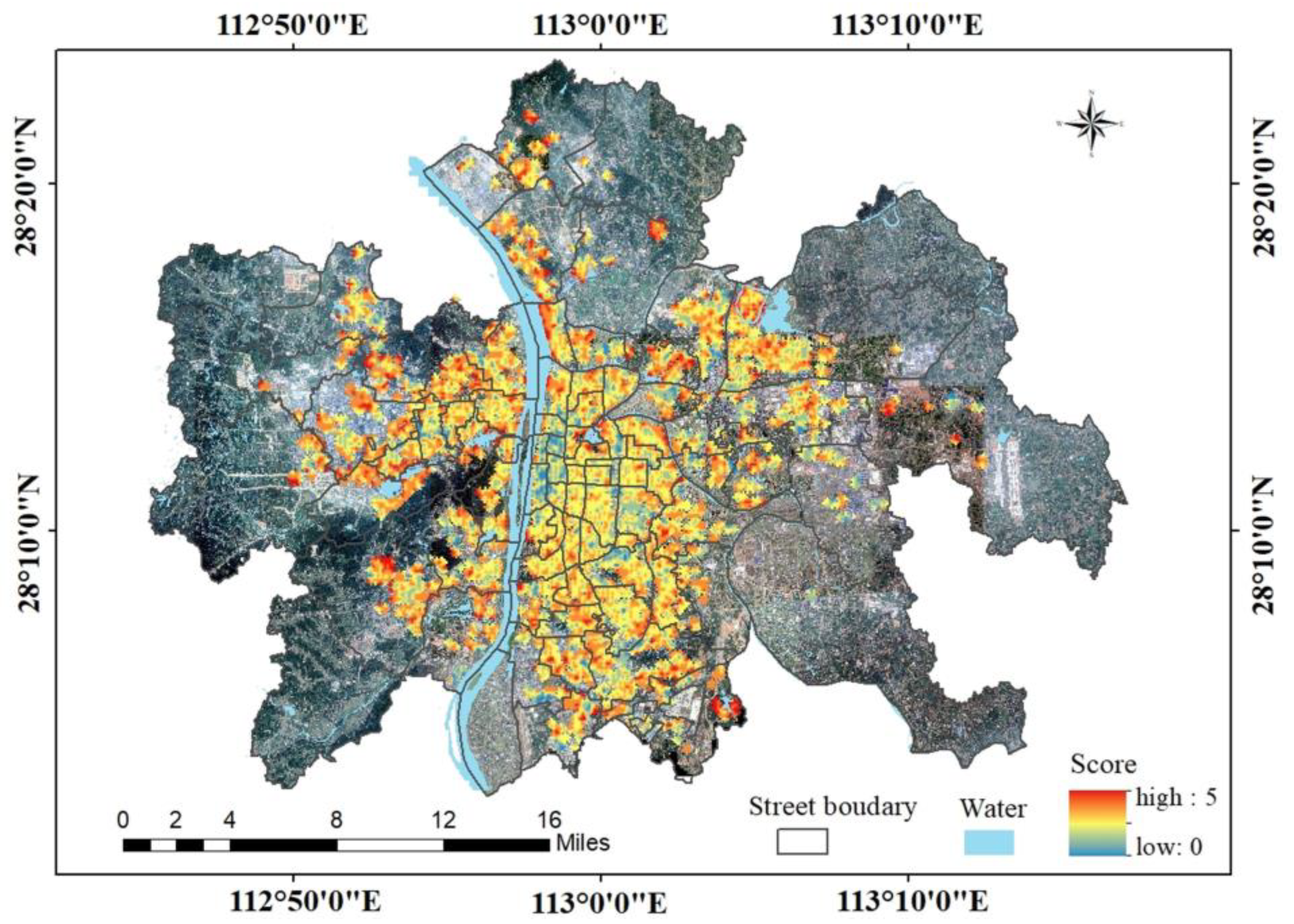
The sampling-point data (Figure 17) were obtained according to the steps described in Section 2.4, and the attribute of the point data was the corresponding environmental-quality-assessment score. After interpolation, the quality-assessment map of the central urban area of Changsha was obtained (Figure 18).
Figure 18 shows the spatial heterogeneity of the environment in the central urban area of Changsha. The figure shows that there is a small blue region on the east bank of the Xiang River. This area is the old urban district of Changsha, where the construction period is relatively old, the residential environment is relatively poor, the commercial activities are rich, the population density is high, and the houses are close to each other. The performance in the five indicators was high building density, less vegetation coverage, narrow roads, and poor connectivity, so the evaluation score was low. The newly developed areas on the west bank of the Xiang River are more orange–red areas because they have low building density, good greenery, and sufficient leisure facilities. This assessment result can simulate the evaluation of human cognition, reflect environmental factors such as building density and vegetation coverage that people pay attention to when choosing a residential area, and provide scientific references for people.
Here, the effectiveness of our generated environment-quality-assessment map is demonstrated by presenting the results on a finer scale. This paper took the road as the boundary and selected six representative regions, a, b, c, d, e, and f, to display the results. The location of each region is shown in Figure 19.
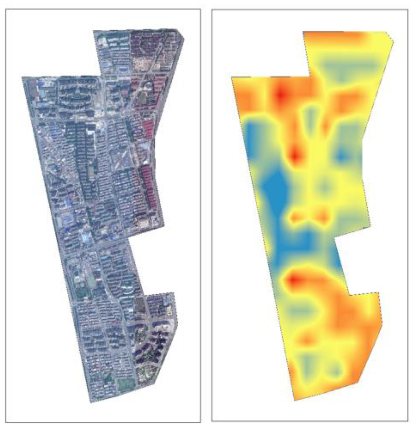
The specific assessment results for the six different location regions are shown in the following figures. Figure 20 shows that the red areas were mainly concentrated in the upper left and lower-right areas, and the middle-left area had lower assessment results. Near the reddest area in the lower right of the figure is a playground, which is one of the few activity areas in this area. In addition, this area has high vegetation coverage, so the assessment result was high.
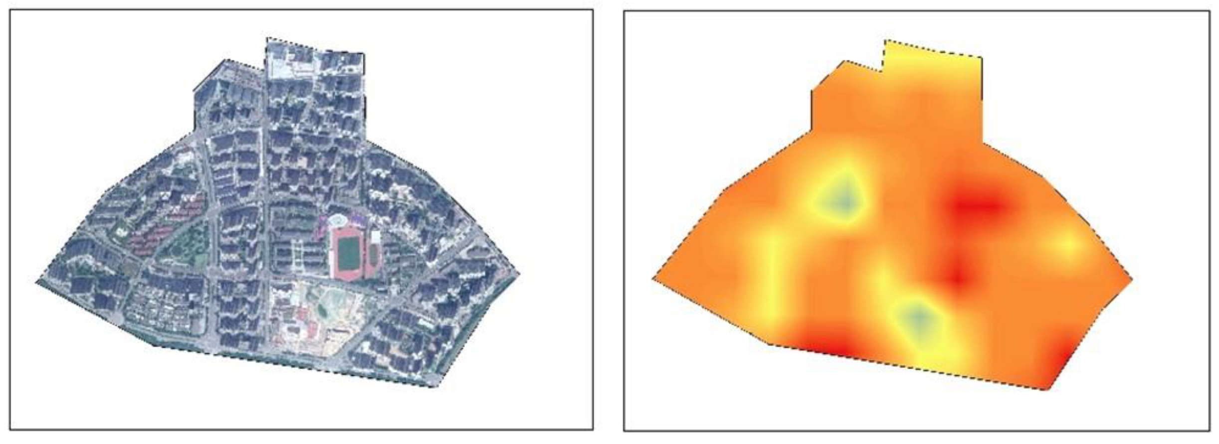
For region b, most of the areas were warm in color, and most of these areas are emerging residential areas (Figure 21). The buildings are open, the vegetation cover is high, and the road connectivity is good. The reddest area corresponds to the location of the playground in the remote-sensing imagery, and it scored higher than the others because of this activity area. The cool-colored area near the bottom corresponds to the area under construction, which is mostly bare land and lacks vegetation coverage, so the score was low.
For region c, the warm-colored areas were mainly concentrated in the middle and right regions, whereas the cool-colored areas were mainly concentrated in the left region (Figure 22). The buildings in the left region are cluttered, with high density, less vegetation coverage, and very poor road connectivity. In contrast, the middle and right areas are relatively neatly arranged, and the road connectivity is slightly better. In general, region c has a high building density and no activity areas, so its overall score was not high.
Region d had three warm-color areas (Figure 23). The warm-color area with the highest score was concentrated at the bottom. In the remote-sensing images, buildings in this area are well arranged, the vegetation is sufficient, and lakes are present, so the scores were higher. The other two warm-color areas correspond to well-arranged residential areas with playgrounds. The score was higher than the surrounding area because of this activity-space element. Other areas have a higher building density, so the assessment result was lower.
For region e, the color was mostly blue (Figure 24). This result is consistent with the actual situation shown by remote-sensing images. This area is densely built and lacks vegetation cover.
For region f (Figure 25), the warm-color area was mainly concentrated in the upper- and lower-right positions, which correspond to the high-grade residential areas with low building density, orderly houses, and good green coverage. The cool-color area was mainly concentrated in the upper-left area. Industrial areas are around this area and vegetation coverage is lacking, so the assessment result was low.
The results show that high-end residential areas scored higher, and this part of the area was developed later, such as region b, which has better greening conditions, building arrangement, and road connectivity. Region e is an area rich in commercial activities. This type of area was developed earlier and is mostly located in the old city. The building density is very high and the greening conditions are poor, so the overall assessment result was low. Although our results do not have clear boundaries, they are good on a fine scale, which can help demonstrate the differences in adjacent locations, discover spatial heterogeneity, and realize assessment at the micro-scale. Moreover, from the overall distribution of the environment-quality-assessment map in Changsha, most of the areas were warm colors and only a few areas were cool colors.

4. Discussion

4.1. Transferability of the Model

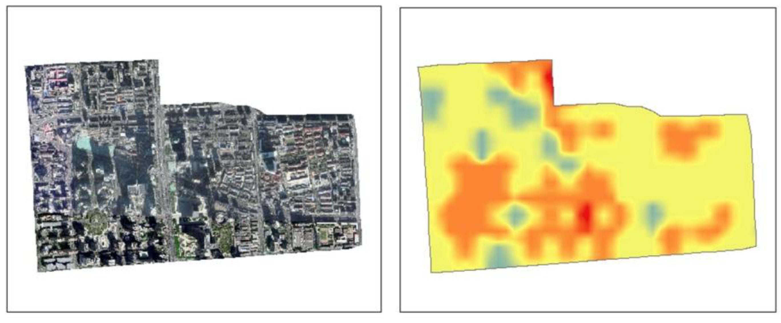
To analyze whether our approach can be effectively applied to other cities, we conducted a built-environment assessment in Chaoyang District of Beijing. Through screening, the urban streets of Chaoyang District, Beijing, were finally selected as the study area (with an area of about 92 km2). Following the steps described above, the final assessment results were obtained. Here, the model trained in Changsha City as described above was used. The final assessment results are shown in Figure 26.
To evaluate the performance of this model in Beijing, blocks a and b were selected for a more detailed analysis. In region a (Figure 27), most of the regions were yellow, and the orange–red areas were mainly concentrated in the lower position. This position corresponds to the residential area with open density and good vegetation coverage in the remote-sensing image, which is also consistent with human cognition. The warm-color areas in region b were mainly concentrated in the left and middle positions (Figure 28). The remote-sensing images show that the distribution of this warm color is consistent with the distribution of the rivers. The orange areas on the right and center correspond to open-plan residential areas close to the river. The red area in the middle corresponds to a relatively open built environment and good vegetation coverage and is close to the river and the playground. In addition, a relatively evident cool-colored area was observed, which corresponds to the industrial area on the right side of the remote-sensing image. According to the above analysis, our method performed well in Chaoyang District and generated assessments that are consistent with human cognition.

4.2. Effectiveness of the Method

The image-description sentences obtained by the image-caption model in this paper is an important base for urban-built-environment assessment. The co-attention module in this model can integrate visual and semantic information and be able to focus on key semantic regions using the attention mechanism. Therefore, we performed an ablation experiment on the co-attention module to evaluate its efficiency.
The experimental results are shown in Table 4, where the i in this table indicates the number of correct sentences among the five description sentences for each image and the P r o p o r t i o n i indicates the proportion of images with i correct sentences to the total number of images in the test set. It can be seen that the number of images with five correct sentences accounted for 85.69% of the number of images in the test set when the co-attention module was used and 74.32% when the co-attention module was not used. Meanwhile, it can also be observed that all other P r o p o r t i o n i (i = 4, 3, 2, 1, 0) increased when the co-attention module was not used, which means that the number of images containing incorrect descriptions increased. For an image scene, if the number of correct description sentences output by the model was not five, the image-caption sentence could not represent the environment objectively enough, resulting in the inability to correctly evaluate the built-up area environment. This shows that the co-attention module plays an important role in generating correct descriptive sentences and obtaining an objective assessment of the built-up area environment.
In addition, this paper provides a new idea for studying environmental-quality assessment from a visual perspective. Owing to the increasing availability of open satellite data and related products, the method presented in this paper has significant potential. This paper also has the following special features:
Firstly, this paper uses natural language to represent geographic entities and their relationships that reflect environmental quality, which is the first attempt in the field of urban-built-environment assessment. The computer is endowed with environmental cognition and realizes natural-language expression. As a medium of human expression, natural language is related to human cognition and is a powerful tool for communicating objective reality and subjective feelings [72]. For the general public, most of the information involved in life is also expressed in natural language. By expressing professional geographic data in natural language, it can be better understood by the public and better serve people without relevant professional backgrounds. Moreover, people’s attention can be limited to a specific fine scale, and local areas can be localized according to needs.
Secondly, the assessment criteria in this paper can better consider the spatial layout and physical characteristics. For example, in the road-connectivity indicators, the road connectivity is considered by the road-layout structure in the scene [49]. Traditional road-related indicators often use road-network density to represent connectivity, but this method has limitations. For example, in the case of excessive intersections or many dead-ends and T-roads, although the road-network density is high, the road-network connectivity is not good, which cannot accurately reflect the real situation within the scene. In addition, for vegetation, which is a common element of residential areas, the assessment criteria in this study make a more detailed distinction, distinguishing between the trees around the building and the forest near the building area. Previous studies [73] generally used values such as NDVI to reflect vegetation coverage. Although it can reflect the overall vegetation coverage of the region, it cannot reflect the vegetation distribution. For example, there may be cases where there is no vegetation coverage in the building area, but the calculated value of the overall vegetation coverage is high due to reasons such as proximity to the forest. The evaluation method in this paper can most intuitively reflect the human perspective and directly reflect the distribution and organization of physical objects such as buildings, roads, and open spaces in small urban scenes, bringing new insights into environmental evaluation.
Lastly, this paper expands the boundaries of urban remote-sensing applications based on the image-caption technology. Urban remote sensing is an important research content in the two fields of remote-sensing application and urban science. High-spatial-resolution remote-sensing images provide detailed surface-coverage information and rich local-structure information for urban monitoring, analysis, evaluation, and management. Existing urban research based on remote-sensing-image data mainly includes the extraction, identification, and classification of ground objects in remote-sensing images [74,75,76]. Realizing the knowledgeable description and expression of geoscience objects is a difficulty in current applications. This paper creatively starts from the perspective of simulating human cognition, constructs the assessment criteria of geographic scenes under the guidance of expert knowledge, and uses image-caption models to express cognition.

4.3. Limitations of the Method

This paper still has certain limitations. First, it only considers the physical environment and assesses the local environmental quality from a visual perspective, ignoring the effect of social, ecological, economic, and cultural conditions. In the future, a more comprehensive discussion should be carried out by combining remote-sensing images with crowd-sourced perception data, social-survey data, and open-source geographic information. Second, this work focuses on the simulation of human expressions. From the perspective of natural-language assessment, the indicators cannot be calculated to obtain quantitative values, which may lead to situations where details cannot be obtained. Future work needs to determine how to perform a more detailed assessment while considering the advantages of natural language. Third, the dataset was labeled by 10 GIS students, and although training and strict quality control were conducted, the limitations of the labeling group may have brought a subjective effect to the data, which may have affected the experimental results.

5. Conclusions

This paper uses high-resolution remote-sensing images as data sources to carry out urban-built-environment assessment from a new perspective. It uses the image-caption model to extract objective scene information and develop a large-scale automatic assessment. It reduces the influence of cropping by adopting an inverse distance-weighted interpolation method. This paper is the first work to apply an image-caption model to urban-built-environment assessment. The contributions of this paper are as follows: (1) According to the characteristics of high-resolution remote-sensing images, it selects representative indicators and defines spatial-assessment criteria of geographic scenes based on high-resolution remote-sensing images. (2) According to the established criteria, it designs an expression framework based on natural language and establishes a dataset, which is the first natural-language dataset established for the application of urban-built-environment assessment. (3) It performs the automatic assessment of large-scale urban built environment by applying an advanced image-caption model. The experimental results demonstrate that our method is effective and transferable for rapid assessment of the urban built environment. This work has also generated an environmental-quality-assessment map in the study area, from which local residents can learn about the high quality of the urban built environment. By looking at the map, planners and city managers can gain a more detailed and comprehensive understanding of the city’s environment and support policy formulation in areas such as urban renewal and community revitalization.
The spatial-assessment criteria of geographic scenes are determined by referring to expert knowledge and visual representation of geographical elements in remote-sensing images. In future work, the setting of evaluation criteria will take into account the requirements of environmental psychology, that is, the establishment of evaluation criteria based on residents’ perceptual feedback on image scenes.

Author Contributions

Conceptualization, J.C. and G.S.; methodology, G.S. and X.D.; software, Y.G.; validation, X.D., J.Z. and X.M.; formal analysis, Y.G. and J.Z.; investigation, X.D.; resources, X.D.; data curation, G.S. and X.M.; writing—original draft preparation, X.D.; writing—review and editing, J.C.; visualization, X.D. and J.Z.; supervision, M.D.; funding acquisition, J.C. All authors have read and agreed to the published version of the manuscript.

Funding

This research was funded by the National Natural Science Foundation of China, grant 42071427; in part by the National Key Research and Development Program of China, grant 2020YFA0713503; and in part by the Central South University Research Programme of Advanced Interdisciplinary Studies, grant 2023QYJC033.

Data Availability Statement

The data that support this study are available from authors, upon reasonable request.

Conflicts of Interest

The authors declare no conflict of interest.

References

  1. Ewing, R.; Cervero, R. Travel and the Built Environment: A Synthesis. Transp. Res. Rec. J. Transp. Res. Board 2001, 1780, 87–114. [Google Scholar] [CrossRef] [Green Version]
  2. Handy, S.L.; Boarnet, M.G.; Ewing, R.; Killingsworth, R.E. How the built environment affects physical activity: Views from urban planning. Am. J. Prev. Med. 2002, 23, 64–73. [Google Scholar] [CrossRef] [PubMed]
  3. Pacione, M. Urban environmental quality and human wellbeing—A social geographical perspective. Landsc. Urban Plan. 2003, 65, 19–30. [Google Scholar] [CrossRef]
  4. Ewing, R.; Handy, S. Measuring the Unmeasurable: Urban Design Qualities Related to Walkability. J. Urban Des. 2009, 14, 65–84. [Google Scholar] [CrossRef]
  5. Marans, R.W.; Stimson, R. An Overview of Quality of Urban Life. In Investigating Quality of Urban Life: Theory, Methods, and Empirical Research; Marans, R.W., Stimson, R.J., Eds.; Springer: Dordrecht, The Netherlands, 2011; pp. 1–29. ISBN 978-94-007-1742-8. [Google Scholar]
  6. Kent, J.L.; Thompson, S. The Three Domains of Urban Planning for Health and Well-being. J. Plan. Lit. 2014, 29, 239–256. [Google Scholar] [CrossRef]
  7. Pfeiffer, D.; Cloutier, S. Planning for Happy Neighborhoods. J. Am. Plan. Assoc. 2016, 82, 267–279. [Google Scholar] [CrossRef]
  8. Wang, F.; Wang, D. Place, Geographical Context and Subjective Well-Being: State of Art and Future Directions. In Mobility, Sociability and Well-being of Urban Living; Wang, D., He, S., Eds.; Springer: Berlin/Heidelberg, Germany, 2016; pp. 189–230. ISBN 978-3-662-48184-4. [Google Scholar]
  9. Mouratidis, K. Rethinking how built environments influence subjective well-being: A new conceptual framework. J. Urban. Int. Res. Placemak. Urban Sustain. 2018, 11, 24–40. [Google Scholar] [CrossRef]
  10. Bahrainy, H.; Khosravi, H. The impact of urban design features and qualities on walkability and health in under-construction environments: The case of Hashtgerd New Town in Iran. Cities 2013, 31, 17–28. [Google Scholar] [CrossRef]
  11. Ding, D.; Gebel, K. Built environment, physical activity, and obesity: What have we learned from reviewing the literature? Health Place 2012, 18, 100–105. [Google Scholar] [CrossRef] [Green Version]
  12. Rodriguez, D.A.; Brisson, E.M.; Estupiñán, N. The relationship between segment-level built environment attributes and pedestrian activity around Bogota’s BRT stations. Transp. Res. Part D Transp. Environ. 2009, 14, 470–478. [Google Scholar] [CrossRef]
  13. Ewing, R.; Hajrasouliha, A.; Neckerman, K.M.; Purciel-Hill, M.; Greene, W. Streetscape Features Related to Pedestrian Activity. J. Plan. Educ. Res. 2016, 36, 5–15. [Google Scholar] [CrossRef] [Green Version]
  14. Park, K.; Ewing, R.; Sabouri, S.; Larsen, J. Street life and the built environment in an auto-oriented US region. Cities 2019, 88, 243–251. [Google Scholar] [CrossRef]
  15. Heath, G.W.; Brownson, R.C.; Kruger, J.; Miles, R.; Powell, K.E.; Ramsey, L.T. The Effectiveness of Urban Design and Land Use and Transport Policies and Practices to Increase Physical Activity: A Systematic Review. J. Phys. Act. Health 2006, 3, S55–S76. [Google Scholar] [CrossRef] [Green Version]
  16. Ameli, S.H.; Hamidi, S.; Garfinkel-Castro, A.; Ewing, R. Do Better Urban Design Qualities Lead to More Walking in Salt Lake City, Utah? J. Urban Des. 2015, 20, 393–410. [Google Scholar] [CrossRef]
  17. McGinn, A.P.; Evenson, K.R.; Herring, A.H.; Huston, S.L.; Rodriguez, D.A. Exploring Associations between Physical Activity and Perceived and Objective Measures of the Built Environment. J. Urban Health 2007, 84, 162–184. [Google Scholar] [CrossRef] [Green Version]
  18. Li, X.; Zhang, C.; Li, W.; Ricard, R.; Meng, Q.; Zhang, W. Assessing street-level urban greenery using Google Street View and a modified green view index. Urban For. Urban Green. 2015, 14, 675–685. [Google Scholar] [CrossRef]
  19. Zhou, H.; He, S.; Cai, Y.; Wang, M.; Su, S. Social inequalities in neighborhood visual walkability: Using street view imagery and deep learning technologies to facilitate healthy city planning. Sustain. Cities Soc. 2019, 50, 101605. [Google Scholar] [CrossRef]
  20. Tang, J.; Long, Y. Measuring visual quality of street space and its temporal variation: Methodology and its application in the Hutong area in Beijing. Landsc. Urban Plan. 2019, 191, 103436. [Google Scholar] [CrossRef]
  21. Wang, R.; Lu, Y.; Zhang, J.; Liu, P.; Yao, Y.; Liu, Y. The relationship between visual enclosure for neighbourhood street walkability and elders’ mental health in China: Using street view images. J. Transp. Health 2019, 13, 90–102. [Google Scholar] [CrossRef]
  22. Hu, C.-B.; Zhang, F.; Gong, F.-Y.; Ratti, C.; Li, X. Classification and mapping of urban canyon geometry using Google Street View images and deep multitask learning. Build. Environ. 2020, 167, 106424. [Google Scholar] [CrossRef]
  23. He, L.; Páez, A.; Liu, D. Built environment and violent crime: An environmental audit approach using Google Street View. Comput. Environ. Urban Syst. 2017, 66, 83–95. [Google Scholar] [CrossRef]
  24. Liu, L.; Silva, E.A.; Wu, C.; Wang, H. A machine learning-based method for the large-scale evaluation of the qualities of the urban environment. Comput. Environ. Urban Syst. 2017, 65, 113–125. [Google Scholar] [CrossRef]
  25. Lu, Y. Using Google Street View to investigate the association between street greenery and physical activity. Landsc. Urban Plan. 2019, 191, 103435. [Google Scholar] [CrossRef]
  26. Wu, C.; Peng, N.; Ma, X.; Li, S.; Rao, J. Assessing multiscale visual appearance characteristics of neighbourhoods using geographically weighted principal component analysis in Shenzhen, China. Comput. Environ. Urban Syst. 2020, 84, 101547. [Google Scholar] [CrossRef]
  27. Ye, Y.; Richards, D.; Lu, Y.; Song, X.; Zhuang, Y.; Zeng, W.; Zhong, T. Measuring daily accessed street greenery: A human-scale approach for informing better urban planning practices. Landsc. Urban Plan. 2019, 191, 103434. [Google Scholar] [CrossRef]
  28. Yin, L.; Cheng, Q.; Wang, Z.; Shao, Z. ‘Big data’ for pedestrian volume: Exploring the use of Google Street View images for pedestrian counts. Appl. Geogr. 2015, 63, 337–345. [Google Scholar] [CrossRef]
  29. Zhang, F.; Zhou, B.; Liu, L.; Liu, Y.; Fung, H.H.; Lin, H.; Ratti, C. Measuring human perceptions of a large-scale urban region using machine learning. Landsc. Urban Plan. 2018, 180, 148–160. [Google Scholar] [CrossRef]
  30. Larkin, A.; Gu, X.; Chen, L.; Hystad, P. Predicting perceptions of the built environment using GIS, satellite and street view image approaches. Landsc. Urban Plan. 2021, 216, 104257. [Google Scholar] [CrossRef] [PubMed]
  31. Zhang, Y.; Chen, N.; Du, W.; Li, Y.; Zheng, X. Multi-source sensor based urban habitat and resident health sensing: A case study of Wuhan, China. Build. Environ. 2021, 198, 107883. [Google Scholar] [CrossRef] [PubMed]
  32. De Sa, E.; Ardern, C.I. Neighbourhood walkability, leisure-time and transport-related physical activity in a mixed urban–rural area. Peerj 2014, 2, e440. [Google Scholar] [CrossRef] [PubMed] [Green Version]
  33. Omuta, G.E.D. The quality of urban life and the perception of livability: A case study of neighbourhoods in Benin City, Nigeria. Soc. Indic. Res. 1988, 20, 417–440. [Google Scholar] [CrossRef]
  34. Klopp, J.M.; Petretta, D.L. The urban sustainable development goal: Indicators, complexity and the politics of measuring cities. Cities 2017, 63, 92–97. [Google Scholar] [CrossRef]
  35. Leach, J.M.; Lee, S.E.; Hunt, D.V.L.; Rogers, C.D.F. Improving city-scale measures of livable sustainability: A study of urban measurement and assessment through application to the city of Birmingham, UK. Cities 2017, 71, 80–87. [Google Scholar] [CrossRef]
  36. Lynch, A.J.; Mosbah, S.M. Improving local measures of sustainability: A study of built-environment indicators in the United States. Cities 2017, 60, 301–313. [Google Scholar] [CrossRef]
  37. Paul, A.; Sen, J. Livability assessment within a metropolis based on the impact of integrated urban geographic factors (IUGFs) on clustering urban centers of Kolkata. Cities 2018, 74, 142–150. [Google Scholar] [CrossRef]
  38. Shafer, C.S.; Lee, B.K.; Turner, S. A tale of three greenway trails: User perceptions related to quality of life. Landsc. Urban Plan. 2000, 49, 163–178. [Google Scholar] [CrossRef]
  39. Krause, J.; Johnson, J.; Krishna, R.; Fei-Fei, L. A Hierarchical Approach for Generating Descriptive Image Paragraphs. In Proceedings of the 2017 IEEE Conference on Computer Vision and Pattern Recognition (CVPR), Honolulu, HI, USA, 21–26 July 2017; pp. 317–325. [Google Scholar] [CrossRef] [Green Version]
  40. Blaschke, T.; Merschdorf, H.; Cabrera-Barona, P.; Gao, S.; Papadakis, E.; Kovacs-Györi, A. Place versus Space: From Points, Lines and Polygons in GIS to Place-Based Representations Reflecting Language and Culture. ISPRS Int. J. Geo-Inf. 2018, 7, 452. [Google Scholar] [CrossRef] [Green Version]
  41. Rosner, T.; Curtin, K.M. Quantifying Urban Diversity: Multiple Spatial Measures of Physical, Social, and Economic Characteristics. In Computational Approaches for Urban Environments; Helbich, M., Jokar Arsanjani, J., Leitner, M., Eds.; Springer International Publishing: Cham, Switzerland, 2015; pp. 149–181. ISBN 978-3-319-11469-9. [Google Scholar]
  42. Koroleva, P.; Chichkova, N.; Mityagin, S.A. Modeling and evaluating the residential urban environment perception. Procedia Comput. Sci. 2020, 178, 103–115. [Google Scholar] [CrossRef]
  43. Hur, M.; Morrow-Jones, H. Factors That Influence Residents’ Satisfaction with Neighborhoods. Environ. Behav. 2008, 40, 619–635. [Google Scholar] [CrossRef]
  44. Hur, M.; Nasar, J.L.; Chun, B. Neighborhood satisfaction, physical and perceived naturalness and openness. J. Environ. Psychol. 2010, 30, 52–59. [Google Scholar] [CrossRef]
  45. Al-Thani, S.K.; Amato, A.; Koç, M.; Al-Ghamdi, S.G. Urban Sustainability and Livability: An Analysis of Doha’s Urban-form and Possible Mitigation Strategies. Sustainability 2019, 11, 786. [Google Scholar] [CrossRef] [Green Version]
  46. Chan, I.Y.S.; Liu, A.M.M. Effects of neighborhood building density, height, greenspace, and cleanliness on indoor environment and health of building occupants. Build. Environ. 2018, 145, 213–222. [Google Scholar] [CrossRef]
  47. Stewart, I.D.; Oke, T.R. Local Climate Zones for Urban Temperature Studies. Bull. Am. Meteorol. Soc. 2012, 93, 1879–1900. [Google Scholar] [CrossRef]
  48. Wei, Y.D.; Xiao, W.; Wen, M.; Wei, R. Walkability, Land Use and Physical Activity. Sustainability 2016, 8, 65. [Google Scholar] [CrossRef] [Green Version]
  49. Duan, Y.; Lei, K.; Tong, H.; Li, B.; Wang, W.; Hou, Q. Land use characteristics of Xi’an residential blocks based on pedestrian traffic system. Alex. Eng. J. 2021, 60, 15–24. [Google Scholar] [CrossRef]
  50. Malambo, P.; Kengne, A.P.; De Villiers, A.; Lambert, E.V.; Puoane, T. Built Environment, Selected Risk Factors and Major Cardiovascular Disease Outcomes: A Systematic Review. PLoS ONE 2016, 11, e0166846. [Google Scholar] [CrossRef] [Green Version]
  51. Xu, L.; Xu, H.; Wang, T.; Yue, W.; Deng, J.; Mao, L. Measuring Urban Spatial Activity Structures: A Comparative Analysis. Sustainability 2019, 11, 7085. [Google Scholar] [CrossRef] [Green Version]
  52. Sharifi, A. Resilient urban forms: A review of literature on streets and street networks. Build. Environ. 2019, 147, 171–187. [Google Scholar] [CrossRef]
  53. Yan, M.; Li, H.; Fang, Y.; Wang, Y. Modeling on Environmental Quality Evaluation for Urban Residential Area by High Resolution Remote Sensing Classification Informatics. In Proceedings of the 2016 4th International Workshop on Earth Observation and Remote Sensing Applications (EORSA), Guangzhou, China, 4–6 July 2016; pp. 309–313. [Google Scholar]
  54. Yan, M.; Ren, L.; He, X.; Sang, W. Evaluation of Urban Environmental Quality with High Resolution Satellite Images. In Proceedings of the IGARSS 2008-2008 IEEE International Geoscience and Remote Sensing Symposium, Boston, MA, USA, 7–11 July 2008; Volume 3, pp. III-1280–III-1283. [Google Scholar]
  55. Zhang, F.; Wu, L.; Zhu, D.; Liu, Y. Social sensing from street-level imagery: A case study in learning spatio-temporal urban mobility patterns. ISPRS J. Photogramm. Remote Sens. 2019, 153, 48–58. [Google Scholar] [CrossRef]
  56. Shao, Q.; Weng, S.-S.; Liou, J.J.H.; Lo, H.-W.; Jiang, H. Developing a Sustainable Urban-Environmental Quality Evaluation System in China Based on a Hybrid Model. Int. J. Environ. Res. Public Health 2019, 16, 1434. [Google Scholar] [CrossRef] [PubMed] [Green Version]
  57. Zhang, Y.; Li, Q.; Huang, H.; Wu, W.; Du, X.; Wang, H. The Combined Use of Remote Sensing and Social Sensing Data in Fine-Grained Urban Land Use Mapping: A Case Study in Beijing, China. Remote Sens. 2017, 9, 865. [Google Scholar] [CrossRef] [Green Version]
  58. Marim, H.M.; Bashir, M.E.; Abdelelah, M.E.; Lgaz, H.; Jodeh, S.; Chetouani, A.; Salghi, R. The Environmental Impacts of Generated Air Pollution in Omdurman Industrial and Residential Area, Khartoum State, Sudan. Moroc. J. Chem. 2016, 4, 4–837. [Google Scholar] [CrossRef]
  59. Shakede, O.P.; Ndubisi, O. Effect of Industrial Pollution on Residential Neighbourhood: Amuwo Odofin Industrial Layout Lagos as Case Study. Covenant J. Res. Built Environ. 2017, 5, 99–106. [Google Scholar]
  60. Martínez-Bravo, M.D.M.; Martínez-Del-Río, J.; Antolín-López, R. Trade-offs among urban sustainability, pollution and livability in European cities. J. Clean. Prod. 2019, 224, 651–660. [Google Scholar] [CrossRef]
  61. Douglas, O.; Russell, P.; Scott, M. Positive perceptions of green and open space as predictors of neighbourhood quality of life: Implications for urban planning across the city region. J. Environ. Plan. Manag. 2019, 62, 626–646. [Google Scholar] [CrossRef]
  62. Ambrey, C.; Fleming, C. Public Greenspace and Life Satisfaction in Urban Australia. Urban Stud. 2014, 51, 1290–1321. [Google Scholar] [CrossRef]
  63. Chandio, I.A.; Matori, A.-N.; Lawal, D.U.; Sabri, S. GIS-based Land Suitability Analysis Using AHP for Public Parks Planning in Larkana City. Mod. Appl. Sci. 2011, 5, 177. [Google Scholar] [CrossRef] [Green Version]
  64. Fu, B.; Yu, D.; Zhang, Y. The livable urban landscape: GIS and remote sensing extracted land use assessment for urban livability in Changchun Proper, China. Land Use Policy 2019, 87, 104048. [Google Scholar] [CrossRef]
  65. Chen, J.; Han, Y.; Wan, L.; Zhou, X.; Deng, M. Geospatial relation captioning for high-spatial-resolution images by using an attention-based neural network. Int. J. Remote Sens. 2019, 40, 6482–6498. [Google Scholar] [CrossRef]
  66. Cui, W.; Zhang, D.; He, X.; Yao, M.; Wang, Z.; Hao, Y.; Li, J.; Wu, W.; Cui, W.; Huang, J. Multi-Scale Remote Sensing Semantic Analysis Based on a Global Perspective. ISPRS Int. J. Geo-Inf. 2019, 8, 417. [Google Scholar] [CrossRef] [Green Version]
  67. Qu, B.; Li, X.; Tao, D.; Lu, X. Deep semantic understanding of high resolution remote sensing image. In Proceedings of the 2016 International Conference on Computer, Information and Telecommunication Systems (CITS), Kunming, China, 6–8 July 2016; pp. 1–5. [Google Scholar] [CrossRef]
  68. Shi, Z.; Zou, Z. Can a Machine Generate Humanlike Language Descriptions for a Remote Sensing Image? IEEE Trans. Geosci. Remote Sens. 2017, 55, 3623–3634. [Google Scholar] [CrossRef]
  69. Wang, B.; Lu, X.; Zheng, X.; Li, X. Semantic Descriptions of High-Resolution Remote Sensing Images. IEEE Geosci. Remote Sens. Lett. 2019, 16, 1274–1278. [Google Scholar] [CrossRef]
  70. Jing, B.; Xie, P.; Xing, E. On the Automatic Generation of Medical Imaging Reports. In Proceedings of the 56th Annual Meeting of the Association for Computational Linguistics, Melbourne, Australia, 15–20 July 2018; pp. 2577–2586. [Google Scholar]
  71. Ahn, S.; Chung, S.-R.; Oh, H.-J.; Chung, C.-Y. Composite Aerosol Optical Depth Mapping over Northeast Asia from GEO-LEO Satellite Observations. Remote Sens. 2021, 13, 1096. [Google Scholar] [CrossRef]
  72. Sap, M.; Horvitz, E.; Choi, Y.; Smith, N.A.; Pennebaker, J.W. Recollection versus Imagination: Exploring Human Memory and Cognition via Neural Language Models. In Proceedings of the 58th Annual Meeting of the Association for Computational Linguistics, Online, 5–10 July 2020; pp. 1970–1978. [Google Scholar]
  73. Musse, M.A.; Barona, D.A.; Rodriguez, L.M.S. Urban environmental quality assessment using remote sensing and census data. Int. J. Appl. Earth Obs. Geoinf. 2018, 71, 95–108. [Google Scholar] [CrossRef]
  74. Kestur, R.; Farooq, S.; Abdal, R.; Mehraj, E.; Narasipura, O.S.; Mudigere, M. UFCN: A fully convolutional neural network for road extraction in RGB imagery acquired by remote sensing from an unmanned aerial vehicle. J. Appl. Remote Sens. 2018, 12, 016020. [Google Scholar] [CrossRef]
  75. Song, S.; Liu, J.; Liu, Y.; Feng, G.; Han, H.; Yao, Y.; Du, M. Intelligent Object Recognition of Urban Water Bodies Based on Deep Learning for Multi-Source and Multi-Temporal High Spatial Resolution Remote Sensing Imagery. Sensors 2020, 20, 397. [Google Scholar] [CrossRef] [Green Version]
  76. Zhou, D.; Wang, G.; He, G.; Yin, R.; Long, T.; Zhang, Z.; Chen, S.-B.; Luo, B. A Large-Scale Mapping Scheme for Urban Building from Gaofen-2 Images Using Deep Learning and Hierarchical Approach. IEEE J. Sel. Top. Appl. Earth Obs. Remote Sens. 2021, 14, 11530–11545. [Google Scholar] [CrossRef]
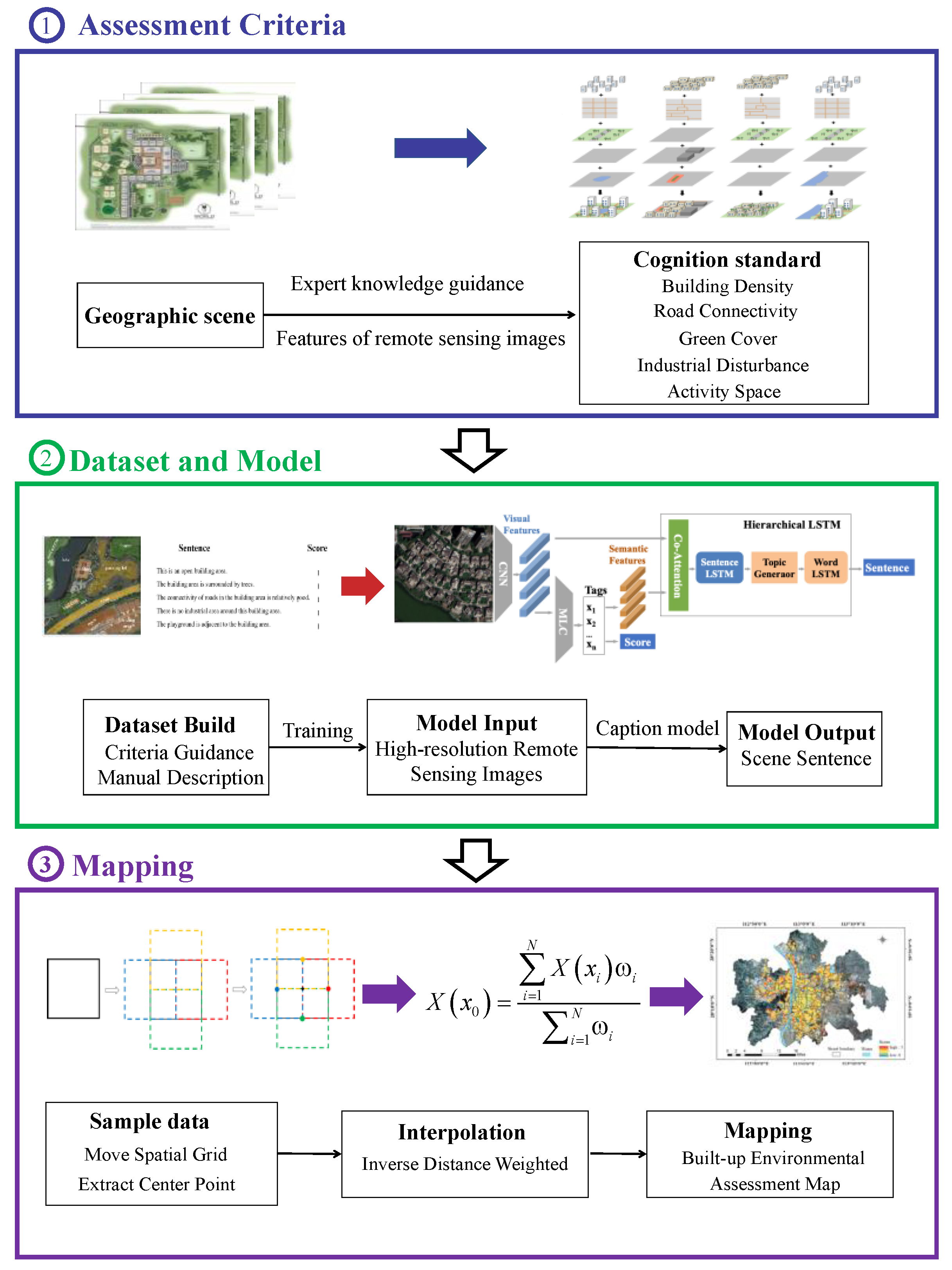
Figure 1. The proposed environment-assessment framework.
Remotesensing 15 01436 g001
Figure 2. Different urban built environments composed of visual elements.
Remotesensing 15 01436 g002
Figure 3. Image patches with different spatial extents of (a) 125 × 125, (b) 250 × 250, and (c) 500 × 500.
Remotesensing 15 01436 g003
Figure 4. Image filtering (a) water area, (b) woodland, and (c) rural construction area.
Remotesensing 15 01436 g004
Figure 5. Construction of a sketch.
Remotesensing 15 01436 g005
Figure 6. Mapping of sketch to natural language.
Remotesensing 15 01436 g006
Figure 7. Model-structure diagram.
Remotesensing 15 01436 g007
Figure 8. Effect of cropping. (a) An industrial area is located within a spatial-grid unit. (b) An industrial area is located outside but adjacent to a spatial-grid unit.
Remotesensing 15 01436 g008
Figure 9. Spatial-grid-unit movement and point extraction.
Remotesensing 15 01436 g009
Figure 10. Remote-sensing image and building-outline maps.
Remotesensing 15 01436 g010
Figure 11. Example of scene units with scores of 5.
Remotesensing 15 01436 g011
Figure 12. Example of scene units with scores of 4.
Remotesensing 15 01436 g012
Figure 13. Example of scene unis with scores of 3.
Remotesensing 15 01436 g013
Figure 14. Example of scene units with scores of 2.
Remotesensing 15 01436 g014
Figure 15. Example of scene units with scores of 1.
Remotesensing 15 01436 g015
Figure 16. Example of scene units with scores of 0.
Remotesensing 15 01436 g016
Figure 17. Distribution of sampling points.
Remotesensing 15 01436 g017
Figure 18. Environmental-quality-assessment map.
Remotesensing 15 01436 g018
Figure 19. Location map of six regions. The specific assessment result for region (af).
Remotesensing 15 01436 g019
Figure 20. Assessment result of region a.
Remotesensing 15 01436 g020
Figure 21. Assessment result of region b.
Remotesensing 15 01436 g021
Figure 22. Assessment result of region c.
Remotesensing 15 01436 g022
Figure 23. Assessment result of region d.
Remotesensing 15 01436 g023
Figure 24. Assessment result of region e.
Remotesensing 15 01436 g024
Figure 25. Assessment result of region f.
Remotesensing 15 01436 g025
Figure 26. Environmental-assessment map of several streets in Chaoyang District. The specific assessment result for region (a,b) in Chaoyang District.
Remotesensing 15 01436 g026
Figure 27. Assessment results of region a in Chaoyang District.
Remotesensing 15 01436 g027
Figure 28. Assessment results of region b in Chaoyang District.
Remotesensing 15 01436 g028
Table 1. Assessment criteria for remote-sensing-image scenes.
IndicatorCriteriaComprehensive Score
Building density1: Low density and open layout X = i = 1 5 x i
The range is 0–5 points
0: High density and compact layout
Road connectivity1: Grid structure
0: Tree structure
Vegetation coverage1: Vegetation coverage
0: No vegetation coverage
Distribution of industrial area1: No distribution of industrial area
0: Distribution of industrial area
Distribution of activity area 1: Distribution of forest
1: Distribution of lake
1: Distribution of river
1: Distribution of playground
0: No distribution of activity area
Table 2. Assessment accuracy for pictures.
i N i Proportion1
552785.69%
47712.52%
391.46%
220.33%
100
000
Table 3. Assessment accuracy for indicators.
j N j Proportion2
Building57393.17%
Vegetation59797.07%
Road60197.72%
Industrial area60898.86%
Activity space59596.75%
Table 4. Assessment accuracy of the ablation experiment on the co-attention module.
i P r o p o r t i o n i (Co-Attention) P r o p o r t i o n i   (No Co-Attention)
585.69%74.32%
412.52%17.20%
31.46%4.64%
20.33%2.88%
100.80%
000.16%
Disclaimer/Publisher’s Note: The statements, opinions and data contained in all publications are solely those of the individual author(s) and contributor(s) and not of MDPI and/or the editor(s). MDPI and/or the editor(s) disclaim responsibility for any injury to people or property resulting from any ideas, methods, instructions or products referred to in the content.