Unsupervised SAR Image Change Detection Based on Structural Consistency and CFAR Threshold Estimation

Abstract

Despite the remarkable progress made in recent years, until today, the automatic detection of changes in synthetic aperture radar (SAR) images remains a difficult task due to speckle noise. This inherent multiplicative noise tends to increase false alarms and misdetections. As a solution, we developed an unsupervised method that detects SAR changes by analyzing structural differences. By this method, the spatial structure cues of a pixel are represented by a set of similarity weight vectors calculated from the non-local scale of the pixel. The difference image (DI) is then derived by measuring the structural consistency of the corresponding pixels. A new statistical distance that is insensitive to speckle noise was used to measure the similarity weights between patches in order to obtain an accurate structure. It was derived by applying the Nakagami–Rayleigh distribution to a statistical test and customizing the approximation based on change detection. The CFAR threshold estimator in conjunction with the Rayleigh hypothesis was then employed to attenuate the effect of the unimodal histogram of the DI. The results indicated that the proposed method reduces the false alarm rate and improves the kappa and F1-scores, while providing satisfactory visual results.

1. Introduction

Change detection (CD) is the process of detecting change through remote sensing images taken at different times over the same geographic area. SAR imagery has been used more rarely for change detection tasks than optical imagery, but has always been attractive to scholars due to the independence of atmosphere and sunlight conditions. In recent decades, it has received widespread attention, including urban studies [1], environmental monitoring [2], disaster assessment [3], crop management [4], and land cover monitoring [5]. However, the inherent multiplicative speckle noise has always restricted the analysis and application of SAR to change detection tasks [6].

There are various perspectives for classifying change detection (CD). In terms of the data source, CD can be classified as follows: (1) monomodal change detection (MNCD) and multi-modal change detection (MMCD); (2) from the detection strategy: direct change detection and post-classification comparison; (3) from the scale: pixel-based change detection (PBCD) and object-based change detection (OBCD); (4) from the labeling: unsupervised, semi-supervised, and supervised change detection. Despite the diverse categories, the basic steps typically involve three stages [7]: (1) pre-processing; (2) generation of the difference image (DI); (3) analyzing the difference image to generate the change map (CM).

The first step usually encompasses geometric correction, co-registration, and denoising. The purpose is to geographically align the bi-temporal images, as well as to suppress the noise. In the second step, the differences between the dual-temporal images are compared pixel by pixel in order to obtain the difference image (DI) representing the change level. The third step is to discriminate the DI into two groups: “changed” and “unchanged”. The DI generation step and CM generation step are widely emphasized in the study.

In the context of SAR change detection, the suppression of speckle noise by the ratio-based method is an important research trend. In the DI generation step, the main approaches are the ratio detector (RD) [8] and the log-ratio detector (LRD) [9]. For isolated noise pixels, a mean-ratio detector (MRD) [10] incorporating neighborhood information was developed to find changes by the ratio of the mean values of local patches. Additionally, other advanced ratio-based detectors, such as the neighborhood-based ratio detector [11] and the region likelihood ratio detector [12], have been developed to address specific situations.

Later, the combined difference image (CDI) was proposed to enhance detection by fusing the LRD and the MRD. It is based on the consensus that different detectors target different differences. In the work of Ma et al. [13], the authors performed wavelet transforms on the LRD and the MRD and then extracted their high- and low-frequency components, respectively. The final DI was reconstructed by fusing LL, LH, HL, and HH under a neighborhood-based fusion rule. Zheng et al. [14] fused the subtraction DI and the log-ratio DI by experimental trial and error, allowing region consistency and edge information to be retained. In [15], the authors proposed a novel fusion strategy based on the discrete wavelet transform (DWT). The study explored the rule of selecting the weight averaging for the low frequency and the maximum local contrast coefficients for the high frequency. Experience showed that the CDI fusing the log-ratio DI and the Gauss-log ratio DI enhances the difference intensity of the changed area. Later, the work by Gong et al. [16] extended the fusion techniques by constructing intensity–texture difference images (ITIDs). The ITID includes the intensity DI (IDI) and the texture DI (TDI), which are generated by the log-ratio detector and Garbo filter banks. Innovatively, the multivariate generalized Gaussian distribution (MGGD) is employed to fit the joint probability (IDI, TDI), which is used as a prior term in the graph cut. Recently, Wang et al. [17] fused superpixel-level affinities and pixel-level heterogeneous affinities to enhance the multi-scale properties for SAR change detection.

Despite the success of ratio-based methods on CD tasks, they are limited by the properties of first-order statistics and may still fail to detect changes when the average intensity of local neighborhoods remains constant [10]. One possible solution is to use sliding-window-based statistical analysis to consider higher-order neighborhood characteristics. In this mode, changes are detected by measuring the difference of the statistical distribution of each pixel between dual-temporal images. A classical approach is the assumption of a Gaussian distribution under the KL divergence [18]. Subsequently, a local image statistical series expansion method based on cumulants was proposed by Inglada and Mercier [10] to substitute the Gaussian assumption. Immediately afterwards, Zheng and You [19] proposed a projection-based Jeffrey detector (PJD) by replacing the KL divergence with the Jeffrey divergence. More similarity-based CD methods can be found in the work of Alberga [20]. However, since the changes are not modeled, it is difficult to select the window size, which affects the misdetections and overdetections.

In recent years, some scholars have obtained difference images through feature transformation and representation. In this paradigm, the amplitudes are replaced by abstract and reliable features. In [21], the interaction between feature points representing local amplitude attributes was defined as structure features, which were encoded by a graph model based on the ratio similarity. Then, the change can be indicated by the consistency between the graph model constructed on bi-temporal SAR images. In the work of Wan et al. [22], a sort histogram was created for each pixel to implicitly express the local spatial layout, which weakens the defects of the PBCD method. Besides, a pairwise pixel-structure-representing approach was proposed by Touati et al. [23] for the heterogeneous CD task. It models the observation field through each image’s own pixel pairs, which is imaging modality-invariant. Recently, a parametric contraction mapping strategy based on spatial fractal decomposition was proposed in [24] to make dual-temporal images comparable in the presence of intensity heterogeneity. This mapping is based on the consensus that any satellite data can be approximately encoded with their own appropriate spatial transformation part. Moreover, in recent studies, Sun et al. [25] proposed the NLPG method to build a K-nearest graph and a cross-mapping graph for each pixel, whose discrepancy can reflect the change information. Later, an extended version of NLPG, named IRG-McS [26], was put forward based on superpixels and iteration.

The DI analysis step can be viewed as a binary partitioning problem. A decision threshold is usually determined to divide the DI into two categories. The Kittler–Illingworth threshold (K&I) [27], the expectation maximization (EM) threshold, and Otsu [28] are several widely used estimation methods, and they work under the class conditional distribution assumption and no prior distribution assumption, respectively. Besides, empirical threshold selection is also a common approach, which is called “trial and error” (TAE). Clustering methods such as PCAKmeans [29], FCM, and FLICM [30,31,32], in an unsupervised segmentation manner, automatically aggregate pixels into “change” and “unchanged” classes without modeling the statistical distribution. Meanwhile, the recently proposed new threshold method HFEM outperforms Otsu and FCM in the case of only a few change areas [33].

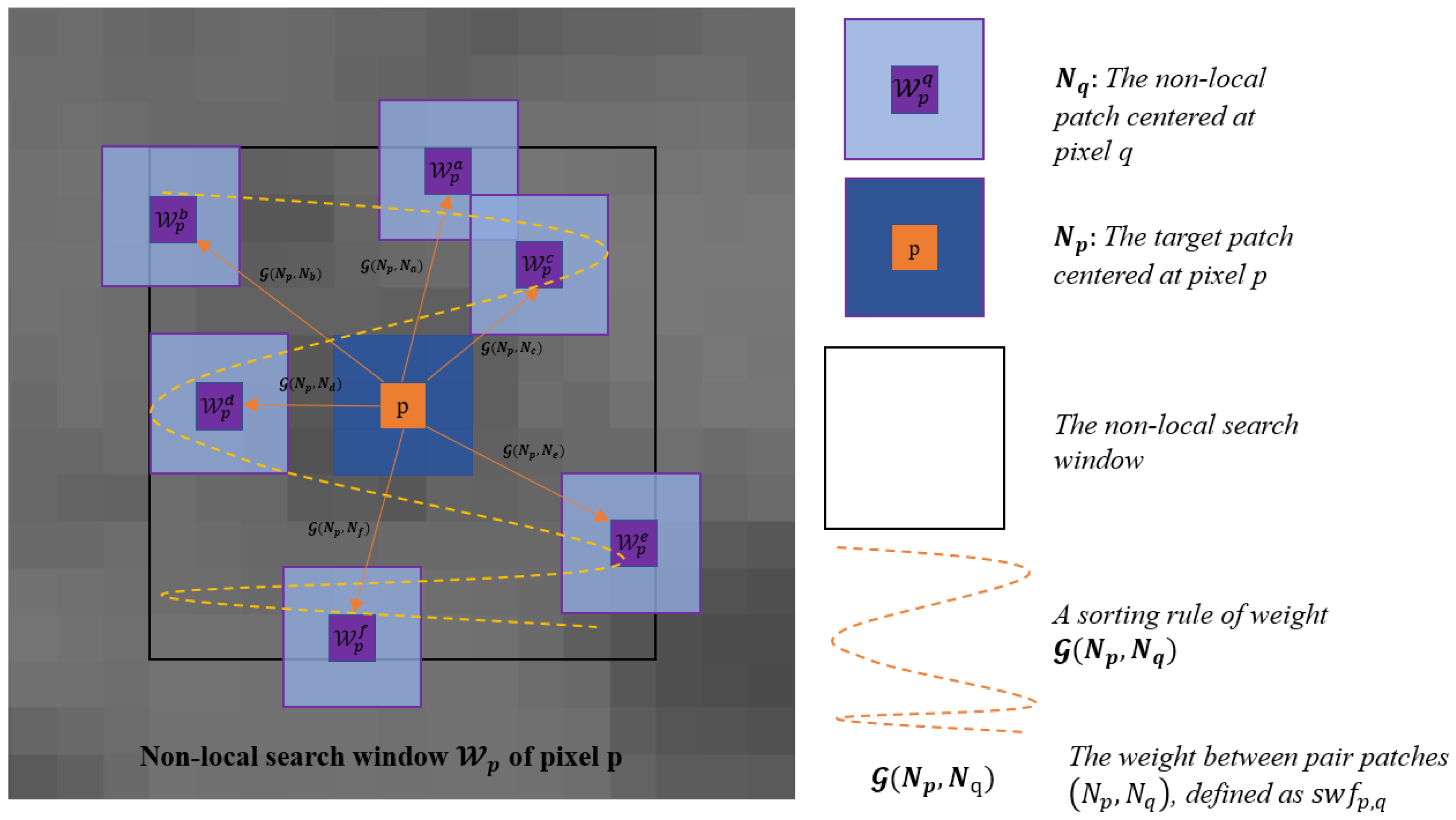
This research focused on improving the performance of the pixel-based change detector in the presence of speckle noise. To this end, we propose an effective method based on the self-similarity of non-local structures. Speckle noise can still produce a large amplitude difference even between pixels pairs that have not changed, even in a monomodal CD task. However, the unchanged areas share the same spatial structure [25]. Inspired by Sun et al. [34,35], we can, therefore, determine whether a pixel has changed by measuring the structural consistency of the corresponding pixels. Unlike them, we focused on SAR change detection. The acquired structural features were dense, i.e., each patch in the non-local scale was taken into account. The spatial structure information of pixels is represented by our proposed non-local structure weight feature (NLSW) and a sorted version (SNLSW). The structure consistency can be measured by the similarity/dissimilarity of NLSW features at the $L_2$-norm.

Each component in the NLSW/SNLSW feature, as the weight strength of the mutual interaction between the center pixel and non-local spatial pixel, is a function of the similarity of their neighborhood patches. The Euclidean distance used in the NLM algorithm is not suitable for SAR due to its inability to accurately construct the strength of the structural weights. To overcome this problem, we derived and approximated a similarity metric suitable for the multiplicative noise model based on our previous work [36], where a dedicated statistical distribution of SAR, i.e., the Nakagami–Rayleigh distribution, was assumed. The derived similarity metric was then used to build the weight components. As a result, pixels associated with changes presented larger differences between the corresponding NLSW/SNLSW features compared to those unchanged pixels.

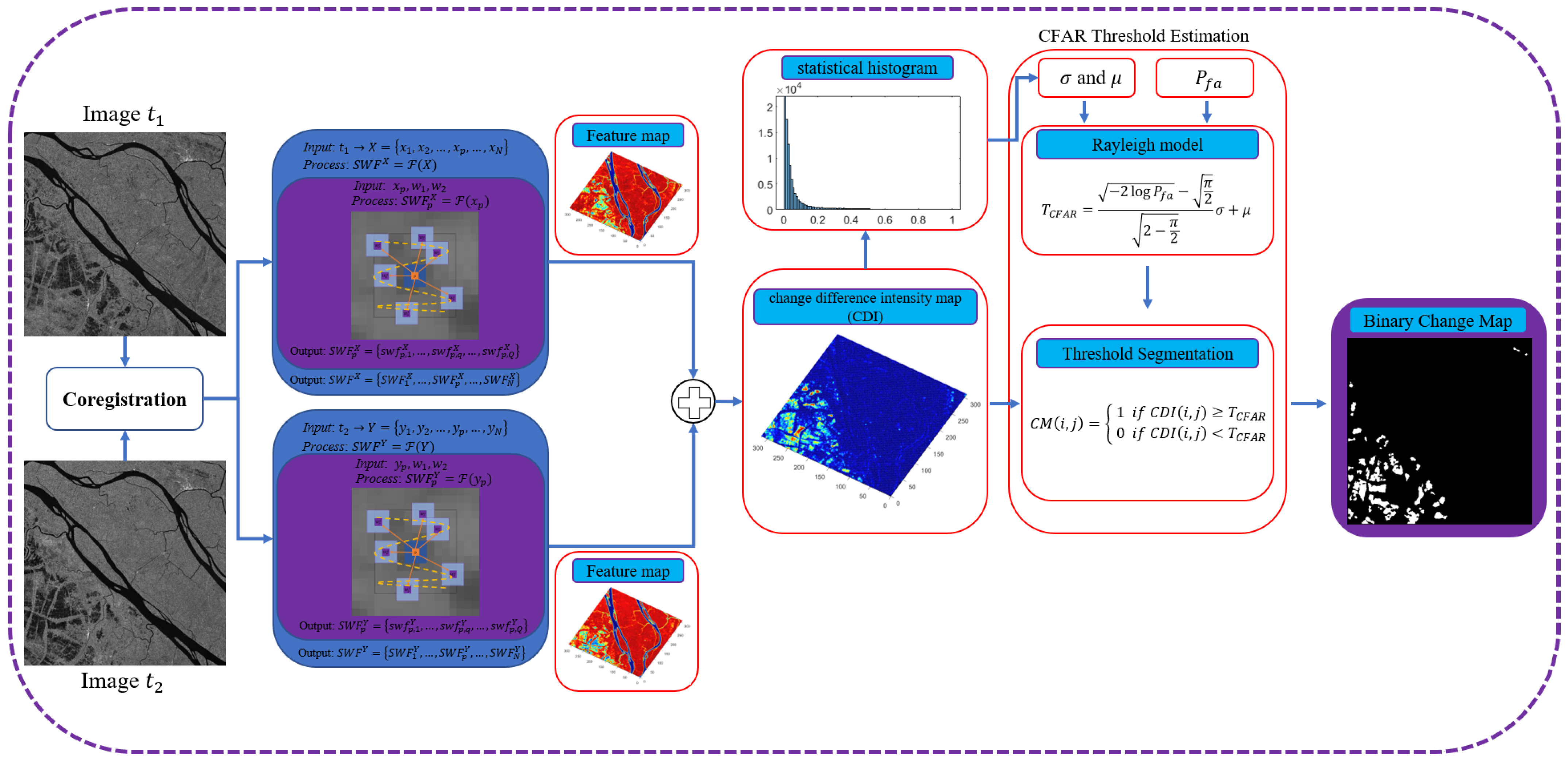
The conversion of the difference image (DI) to the change map (CM) can be regarded as a threshold segmentation procedure. The constant false alarm rate (CFAR) was employed to automatically extract the change areas with an imposed Rayleigh statistical distribution assumption to avoid the difficulty of estimating the decision threshold using histogram-based methods when the change indicator exhibits a unimodal histogram. Besides, the Otsu threshold, K&I threshold, and TAE were also implemented in the DI analysis step.

The main contributions are as follows:

(1)

We propose an unsupervised framework for automated SAR change detection. In the DI generation step, we extract the pixelwise non-local structure weight (NLSW) features and detect changes by spatial structure cues. Eventually, the comparability of bi-temporal SAR images (BTSIs) was enhanced.

(2)

The mathematical proof is given to illustrate the uncertainty of the similarity between patches in the expectation sense when the Euclidean distance is used in multiplicative noise. For this reason, a patch similarity metric, dedicated to the proposed NLSW change detector for BTSIs, was derived and approximated by considering the statistical properties of SAR.

(3)

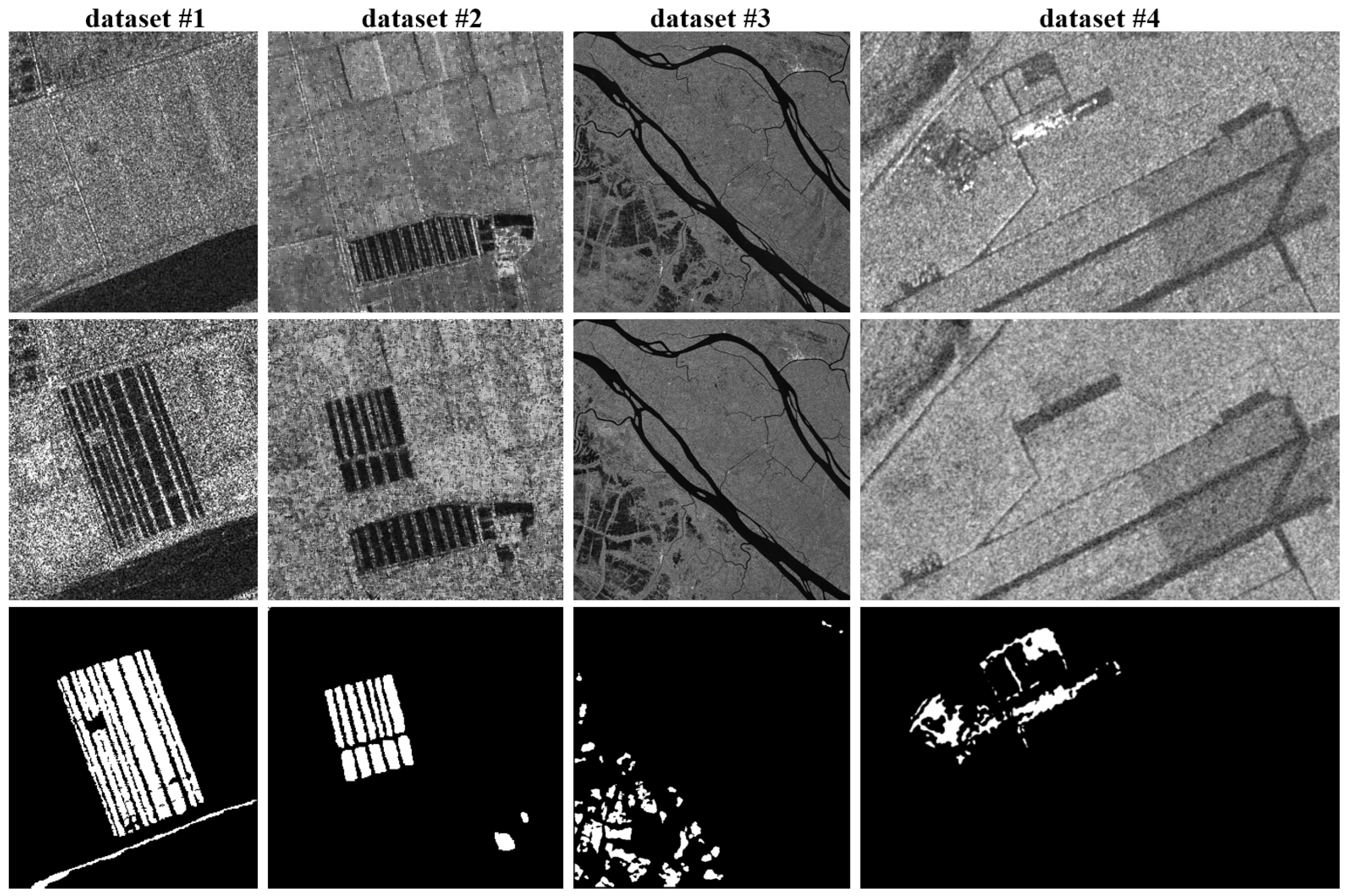
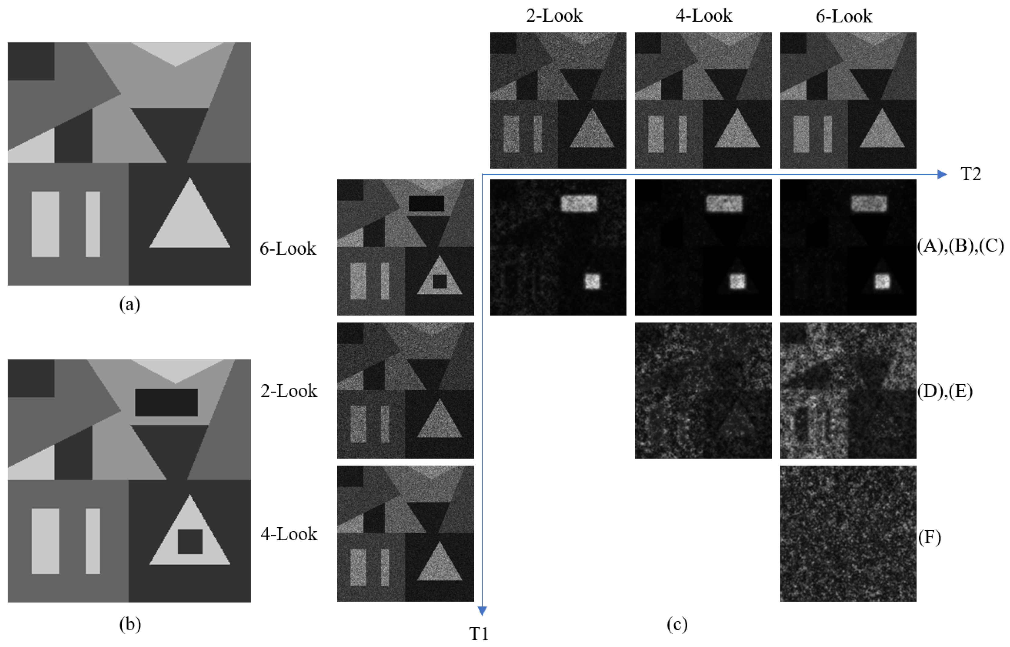
The CFAR under the Rayleigh distribution assumption was applied to the DI to generate the final change map, thus avoiding the unimodal histogram problem. The experiments on simulated and real bi-temporal SAR images demonstrated the effectiveness and stability of the proposed method.

The rest of this paper is organized as follows. Section 2 presents the relevant theories and the proposed framework. Section 3 presents the experimental results, the parameters’ analysis, and the discussion. The conclusion is provided in Section 4.

2. Materials and Methods

Speckle noise is a key factor in accurate change detection of SAR. Due to the fluctuating amplitude, even pixels that have not changed may exhibit significant radiometric differences. The purely amplitude-based methods may fail in highlighting the change area. However, self-similar structures can always be found in any image (common to optical and SAR images). That is, the image can be (approximately) formed of properly transformed parts of itself [24]. One way of constructing self-similar structural information is by applying the idea of non-local means (NLMs) [37]. However, in this work, we were primarily interested in the similarity weights between non-local patches rather than the denoising process of NLMs. This is because the structural information can be well quantified by measuring the similarity between patches’ patterns. Therefore, we built the non-local structure weight (NLSW) feature for each pixel on bi-temporal images by using a set of measured weights in the non-local search window. Figure 1 depicts the construction process of the NLSW feature. We first computed the weight $\mathcal{G}(N_p,N_q)$ (defined in Section 2.2), then we organized all the weights in a certain way (one case is shown by the yellow curve). By assigning the NLSW feature per pixel, a projection of the unstable amplitude space to the stable structural space can be implemented. Then, a simple pixelwise difference between the bi-temporal SAR images can better show the degree of change.

2.1. Theoretical Background

2.1.1. Non-local Means Method

The non-local mean (NLM) is a prevalent image denoising technology that was pioneered by Baudes et al. [38]. The NLM obtains a weighted average of pixels by identifying similar pixels within a non-local spatial search window and then assigning larger weights to those with similar neighboring patterns [39]. In the context of SAR images, the NLM has been shown to be effective at suppressing speckle noise while preserving intricate structural details, thereby facilitating many applications such as SAR segmentation [36], guided patchwise despeckling [40], and OPT/SAR image fusion [41]. Furthermore, the NLM can also improve the resolution and sharpness of SAR images to enhance target detection and identification [42].

In this section, the NLM methods described in [43] are briefly introduced. Let us consider a single-band image $\mathbf{u}={\left(u\left(x\right)\right)}_{x\in \Omega }$ defined over a bounded domain $\Omega \subset {\mathbb{R}}^2$. $u\left(x\right)\subset {\mathbb{R}}_{+}$, $u\left(x\right)$ is the true observed amplitude, i.e., contaminated by noise at pixel $x\in \Omega$. Now, we consider pixel p, then the NLM is defined as

$$\tilde{u}\left(p\right)=\frac{1}{Z\left(p\right)}\sum _{q\in \mathbf{B}(r,p)}w(N_p,N_q)u\left(p\right)$$

(1)

where $N_p$ and $N_q$ represent the neighborhood patch centered at pixel p and pixel q, respectively. $\mathbf{B}(r,p)$ denotes the non-local squared search window centered at pixel p and with a size of $(2r+1)\times (2r+1)$. Limited by the computational cost, q is only chosen within the r-box radius of p. $Z\left(p\right)$ is normalized constant, i.e., $Z\left(p\right)={\sum }_{q\in \mathit{B}(r,p)}w(N_p,N_q)$. The weight $w(N_p,N_q)$ expresses the similarity between the vectorized patches $N_q$ and $N_q$ and is defined as

$$w\left(N_p,N_q\right)=exp-\frac{{∥V_s\left(N_p\right)-V_s\left(N_q\right)∥}_{2,\sigma }^2}{h^2}$$

(2)

where $\sigma$ denotes the standard deviation of the Gaussian kernel, which is used to consider the distance between the central pixel and other pixels in the patch. h is the smoothing parameter, which is usually set empirically. $V_s\left(N_p\right)$ indicates the vectorization of patch $N_p$ with a size of $s\times s$, and $∥·∥$ denotes the ${\ell }_2$-norm.

2.1.2. Euclidean Measurement of Inter-Patches’ Similarity and Problem on SAR Image

The proposed NLSW detector is a structure change indicator based on the self-similarity property, and its accuracy is directly affected by the stability of the weight $w(N_p,N_q)$ in Equation (2). Generally, Equation (2) can provide a fairly reliable estimate of the similarity of patches in optical images (also common to natural images). Azzabou et al. [44] asserted that the Gaussian-weighted similarity estimation (Euclidean distance) is robust for additive noise, but hardly effective for multiplicative noise (SAR speckle). With reference to [45], we introduced a theoretical proof about the validity of the Euclidean distance in optical images and the invalidity in SAR images.

Now, a classical additive noise model is considered, i.e., $Y=X+V$, where Y is the observed image, X is the noise-free image, and V is the zero-mean Gaussian noise with the standard deviation as ${\sigma }_v$. For patches $Y_{N_p}$ and $Y_{N_q}$ centered at the pth and qth pixels, respectively, the distance $\Delta Y_{<p,q>}$ can be written as

$$\Delta Y_{<p,q>}={∥Y_{N_p}-Y_{N_q}∥}_2^2=\sum _{k=1}^O{\left|Y_{N_p}\left(k\right)-Y_{N_q}\left(k\right)\right|}^2$$

(3)

where O denotes the number of pixels in the patch, then the expectation is

$$\begin{array}{cc}\hfill \mathbb{E}\left[\Delta Y_{p,q}\right]& =\mathbb{E}\left[\sum _{k=1}^O{\left|Y_{N_p}\left(k\right)-Y_{N_q}\left(k\right)\right|}^2\right]\hfill \\ \hfill & =\sum _{k=1}^O\mathbb{E}\left\{{\left[\left(X_{N_p}\left(k\right)-X_{N_q}\left(k\right)\right)+\left(V_{N_p}\left(k\right)-V_{N_q}\left(k\right)\right)\right]}^2\right\}\hfill \\ \hfill & =\sum _{k=1}^O\mathbb{E}\left[{\left(\Delta X\left(k\right)+\Delta V\left(k\right)\right)}^2\right]\hfill \\ \hfill & =\sum _{k=1}^O{\left(\Delta X\left(k\right)\right)}^2+\mathbb{E}\left[{\left(\Delta V\left(k\right)\right)}^2\right]\hfill \end{array}$$

(4)

considering $\Delta X\left(k\right)=\left|X_{N_p}\left(k\right)-X_{N_q}\left(k\right)\right|$, and $\Delta V\left(k\right)$ is the difference of the Gaussian distribution, i.e., $\Delta V\sim \mathcal{N}(0,2{\sigma }^2)$, then we can obtain

$$\mathbb{E}\left[\Delta Y_{p,q}\right]={∥X_{N_p}-X_{N_q}∥}_2^2+O·2{\sigma }_v^2$$

(5)

Equation (5) means that the Euclidean distance between the noise-polluted patches $Y_{N_p}$ and $Y_{N_q}$ is related to the similarity between noise-free patches $X_{N_p}$ and $X_{N_q}$, as well as the noise variance ${\sigma }_v$. One can consider that the order of similarity between noise-free patches is preserved in the sense of the distance expectation [45]. That is, if two patches are similar in the absence of noise, they will remain similar in the presence of noise.

From the above evidence, one can see that, for optical images under the additive Gaussian noise model, the Euclidean distance can effectively measure the inter-pixel similarity. However, the SAR image is prone to multiplicative speckle noise, and therefore, Equation (2) no longer fits the SAR image. A multiplicative noise model is assumed for the SAR image, that is $Y=X·V$, where Y denotes the noise-polluted image, X denotes the noise-free image, and V denotes coherent noise with ${\mu }_v=1$ and ${\sigma }_v^2$ the variance. For two patches $Y_{N_p}$ and $Y_{N_q}$, we have the following distance:

$$\Delta Y_{<p,q>}={∥Y_{N_p}-Y_{N_q}∥}_2^2=\sum _{k=1}^O{\left|Y_{N_p}\left(k\right)-Y_{N_q}\left(k\right)\right|}_2^2$$

(6)

then

$$\begin{array}{cc}\hfill \mathbb{E}\left[\Delta Y_{<p,q>}\right]& =\mathbb{E}\left[{∥Y_{N_p}-Y_{N_q}∥}_2^2\right]=\sum _{k=1}^O\mathbb{E}\left[{\left|X_{N_p}\left(k\right)V_{N_p}\left(k\right)-X_{N_q}\left(k\right)V_{N_q}\left(k\right)\right|}^2\right]\hfill \\ \hfill & =\sum _{k=1}^O\mathbb{E}\left[X_{N_p}^2\left(k\right)V_{N_p}^2\left(k\right)-2X_{N_p}\left(k\right)V_{N_p}\left(k\right)X_{N_q}\left(k\right)V_{N_q}\left(k\right)+X_{N_q}^2\left(k\right)V_{N_q}^2\left(k\right)\right]\hfill \\ \hfill & =\sum _{k=1}^O\mathbb{E}\left[X_{N_p}^2\left(k\right)\right]({\sigma }_v^2+1)+\mathbb{E}\left[X_{N_q}^2\left(k\right)\right]({\sigma }_v^2+1)-2\mathbb{E}\left[X_{N_p}\left(k\right)X_{N_q}\left(k\right)\right]\hfill \\ \hfill & =\sum _{k=1}^O{\sigma }_v^2\left(\mathbb{E}\left[X_{N_p}^2\left(k\right)\right]+\mathbb{E}\left[X_{N_q}^2\left(k\right)\right]\right)+\mathbb{E}\left[|X_{N_p}\left(k\right)-X_{N_q}{\left(k\right)|}^2\right]\hfill \\ \hfill & =\sum _{k=1}^O{\left|X_{N_p}\left(k\right)-X_{N_q}\left(k\right)\right|}^2+\sum _{k=1}^O{\sigma }_v^2\left[X_{N_p}^2\left(k\right)+X_{N_q}^2\left(k\right)\right]\hfill \\ \hfill & ={∥X_{N_p}-X_{N_q}∥}_2^2+{\sigma }_v^2\left[\parallel X_{N_p}{\parallel }_2^2+{\parallel X_{N_q}\parallel }_2^2\right]\hfill \end{array}$$

(7)

The second term in Equation (7) indicates that the similarity between the observed patches $Y_{N_p}$ and $Y_{N_q}$ is linked to the noiseless amplitude. This means that the distance depends upon the local area where the patches reside. The larger the amplitude of the local area, the larger the distance between the patches is. As a result, the structural information about SAR obtained from Equation (2) is unstable. To accurately calculate the NLSW features, a distance metric tailored to SAR images should be used.

2.2. A Novel Similarity Measurement for SAR Patches

Precisely projecting the amplitude domain specifically to the structure information domain is the key factor in determining whether the NLSW detector works in the change detection task. It is, of course, inappropriate for SAR to use Equation (2) to calculate the weight similarity. There have been quite a few distance measurements developed in recent years to calculate the similarity of the SAR block. Statistical tests on SAR statistical distributions are a widely discussed topic, such as Deledalle’s proposal in [46]. Based on the statistical properties of SAR images, they summarized a series of distance metrics. Wan et al. [39] applied the Nakagami–Rayleigh distribution to the Bayesian formulation and derived a new statistical distance. Based on their work, we combined the Nakagami–Rayleigh distribution and the generalized likelihood ratio (GLR) to develop a non-logarithmic ratio-based distance in our previous work [36]. This paper introduces this similarity metric in the change detection task due to its decent performance. Significantly, to meet the practical requirements and the computational robustness, we made the following modification.

As a basic theoretical multilook amplitude model for SAR, the Nakagami–Rayleigh distribution was adopted to model the SAR amplitude image [47]. The L-look Nakagami distribution is represented as

$$P\left(X\right|R)=2{\left(\frac{L}{R}\right)}^L\frac{1}{\Gamma \left(L\right)}{X}^{2L-1}exp\left(-L\frac{X^2}{R}\right)$$

(8)

The radar reflectivity, i.e., noise-free pixel amplitude, is represented by R, and the actual observed amplitude is represented by X. $\Gamma \left(·\right)$ is the Gamma function. For paired patches $(N_p,N_q)$, the similarity (or distance) can be statistically regarded as the comparison of two hypothesis, ${\mathcal{H}}_0$ and ${\mathcal{H}}_1$:

$$\begin{array}{cc}\hfill {\mathcal{H}}_0& :R_p=R_q=R_{12}\left(nullhypothesis\right)\hfill \\ \hfill {\mathcal{H}}_1& :R_p\ne R_q\left(alternativehypothesis\right)\hfill \end{array}$$

(9)

where the null hypothesis (${\mathcal{H}}_0$) means that both patches $(N_p,N_q)$ obey the same statistical distribution, i.e., $R_p=R_q=R_{12}$ (parametric constraint). The alternative hypothesis (${\mathcal{H}}_1$) denotes no parametric constraint of R. In this case, the likelihood ratio test (LRT) is the optimal statistical test, which can approximate the ratio of two hypotheses:

$$\mathcal{L}\left(V_s\left(N_p\right),V_s\left(N_q\right)\right)=\frac{P\left(V_s\left(N_p\right),V_s\left(N_q\right)\mid R_p=R_q=R_{12},{\mathcal{H}}_0\right)}{P\left(V_s\left(N_p\right),V_s\left(N_q\right)\mid R_p=R_1,R_q=R_2,{\mathcal{H}}_1\right)}$$

(10)

where $V_s\left(N_p\right)$ and $V_s\left(N_q\right)$ are the observed vectorized patches, which range in $\Theta$. s is the radius of the patches. $R_1$, $R_2$, and $R_{12}$ are the true backscatter values. To limit the range of $\mathit{R}=\{R_1,R_2,R_{12}\}$, the generalized likelihood ratio test (GLRT) extends Equation (10) to address the unknown parameters by using the maximum likelihood estimation (MLE) as if they were known:

$$\mathcal{G}\left(V_s\left(N_p\right),V_s\left(N_q\right)\right)=\underset{\mathit{R}\in \Theta }{Sup}\mathcal{L}\left(V_s\left(N_p\right),V_s\left(N_q\right);\mathit{R}\right)$$

(11)

Note that $\mathcal{G}\left(V_s\left(N_p\right),V_s\left(N_q\right)\right)\in [0,1]$; the larger the value, the greater the confidence in accepting the hypothesis ${\mathcal{H}}_0$ is, which means a higher probability of paired patches $(N_p,N_q)$ obeying the same statistical distribution.

To obtain the analytical solution, we imposed a strict assumption that the paired patches are irrelevant and paired pixels are independent. Thus, Equation (11) can be reformed as

$$\mathcal{G}\left(V_s\left(N_p\right),V_s\left(N_q\right)\right)=\prod _{k=1}^O{\varphi }_{GLR}(x_{p,k},x_{q,k})$$

(12)

where O is $(2s+1)\times (2s+1)$, $x_{p,k}\in N_p$, and $x_{q,k}\in N_q$. ${\varphi }_{GLR}(x_{p,k},x_{q,k})$ is given by

$${\varphi }_{GLR}(x_{p,k},x_{q,k})=\frac{\underset{R_{12}}{Sup}\left\{P\left(x_{p,k},x_{q,k}\mid R_p=R_q=R_{12},{\mathcal{H}}_0\right)\right\}}{\underset{R_1}{Sup}\left\{P\left(x_{p,k}\mid R_p=R_1,{\mathcal{H}}_1\right)\right\}\underset{R_2}{Sup}\left\{P\left(x_{q,k}\mid R_q=R_2,{\mathcal{H}}_1\right)\right\}}$$

(13)

To obtain the maximum likelihood estimation value of the numerator in Equation (13), we define the joint probability $P\left(x_{p,k},x_{q,k}\mid {\mathcal{H}}_0\right)$ by applying Equation (8):

$$P\left(x_{p,k},x_{q,k}\mid {\mathcal{H}}_0\right)={\left(\frac{2}{\Gamma \left(L\right)}\right)}^2{\left(\frac{L}{R_{12}}\right)}^{2L}{\left(x_{p,k}{x}_{q,k}\right)}^{2L-1}exp\left\{-\frac{L}{R_{12}}\left(x_{p,k}^2+x_{q,k}^2\right)\right\}$$

(14)

As for parameter $R_{12}$, we determined its maximum likelihood estimation ${\widehat{R}}_{12}$ by differentiating the log-likelihood function $H\left(R_{12}\right)={\sum }_{m=1}^{M}lnP\left(x_{p,k_m},x_{q,k_m}\mid R_{12}\right)$ and setting $\frac{\mathrm{d}H\left(R_{12}\right)}{\mathrm{d}{R}_{12}}=0$, then we obtain

$${\widehat{R}}_{12}=\frac{1}{2M}\sum _{m=1}^M\left(x_{p,k_m}^2+x_{q,k_m}^2\right)$$

(15)

considering only one pixel can be observed in each position, i.e., $M=1$; therefore, we can obtain the following estimation:

$${\widehat{R}}_{12}=\frac{1}{2}\left(x_{p,k}^2+x_{q,k}^2\right)$$

(16)

For the denominators $P\left(x_{p,k}\mid R_1,{\mathcal{H}}_1\right)$ and $P\left(x_{q,k}\mid R_2,{\mathcal{H}}_1\right)$ in Equation (13), the same estimation process is performed, then we obtain

$$\left\{\begin{array}{c}{\widehat{R}}_1=x_{p,k}^2\hfill \\ {\widehat{R}}_2=x_{p,k}^2\hfill \end{array}\right.$$

(17)

Next, the $\mathit{R}=\left\{R_1,R_2,R_{12}\right\}$ in Equation (13) are replaced by the maximum likelihood estimation $\widehat{\mathit{R}}=\left\{{\widehat{R}}_1,{\widehat{R}}_2,{\widehat{R}}_{12}\right\}$, then we have

$${\varphi }_{GLR}\left(x_{p,k},x_{q,k}\right)=\frac{\frac{4L^{2L}}{\Gamma \left(L\right)}{\left(x_{p,k}{x}_{q,k}\right)}^{2L-1}{(x_{p,k}^2+x_{q,k}^2)}^{-2L}exp(-2L)2^{2L}}{\left\{\frac{2L^L}{\Gamma \left(L\right)}{x}_{p,k}^{-2L}{x}_{p,k}^{2L-1}exp(-L)\right\}\left\{\frac{2L^L}{\Gamma \left(L\right)}{x}_{q,k}^{-2L}{x}_{q,k}^{2L-1}exp(-L)\right\}}$$

(18)

After simplification,

$${\varphi }_{GLR}\left(x_{p,k},x_{q,k}\right)={\left(\frac{2x_{p,k}{x}_{q,k}}{x_{p,k}^2+x_{q,k}^2}\right)}^{2L}$$

(19)

Finally, we can measure the similarity of paired patches $(N_p,N_q)$ by

$$\mathcal{G}\left(N_p,N_q\right)=\prod _{k=1}^O{\varphi }_{GLR}(x_{p,k},x_{q,k})=\prod _{k=1}^O{\left(\frac{2x_{p,k}{x}_{q,k}}{x_{p,k}^2+x_{q,k}^2}\right)}^{2L}$$

(20)

The structure weights can be measured by Equation (20). The statistical distance takes the form of a ratio, so it can suppress speckle noise effectively. However, in this change detection task, we cannot use the continued product form of Equation (20), because it will result in a form that is not computationally tractable and unstable values. Local squared neighborhoods with zero amplitude will result in no similarity, which is not desirable. Our solution to this problem, and to prevent the loss of contrast associated with the logarithmic form, is to approximate the continued product by a summed form.

$$\mathcal{G}\left(N_p,N_q\right)\propto \sum _{k=1}^K{\left(\frac{2x_{p,k}{x}_{q,k}}{x_{p,k}^2+x_{q,k}^2}\right)}^{2L}$$

(21)

2.3. The Non-Local Structure Weight Difference Detector

2.3.1. The Non-Local Structure Weight Feature

Consider two registered SAR images acquired at time $t_1$ and $t_2$ on the same geographical area with a size of $H\times W$, which are represented as $\mathit{X}=\left\{x_1,x_2,\dots ,x_N\right\}$ and $\mathit{Y}=\left\{y_1,y_2,\dots ,y_N\right\}$, respectively. N is the total pixels number. The $N_p$ refers to the patch centered at the pth pixel with a size of $s\times s$. We define ${\mathcal{W}}_p$ as a non-local search window of size $Q=(2w+1)\times (2w+1)$. $\mathbb{P}=\left\{N_q\mid \left(|p_r-q_r|,|p_c-q_c|\right)\in {\mathcal{W}}_p\right\}$ indicates the set of non-local patches in the search window of pixel p. $(r,c)$ denotes the position of the pixels. For the pth pixel in image $\mathit{X}$, the non-local structure weight feature (SWF) is

$${\mathit{SWF}}_{\mathit{p}}^{\mathit{X}}=\left\{sw{f}_{p,1}^X,sw{f}_{p,2}^X,\dots ,sw{f}_{p,q}^X,\dots ,sw{f}_{p,Q-1}^X,sw{f}_{p,Q}^X\right\}$$

(22)

where each element $sw{f}_{p,q}^X$ of Q-dimensional ${\mathit{SWF}}_{\mathit{p}}^{\mathit{X}}$ encodes the distance between the central patch $N_p$ and the corresponding candidate patch $N_q$ in set $\mathbb{P}$. According to the modified distance metric Equation (21), $sw{f}_{p,q}^X$ can be calculated by

$$sw{f}_{p,q}^X=\mathcal{G}\left(N_p,N_q\right)$$

(23)

Traversing each pixel of the bi-temporal SAR images, we can obtain the non-local structure weight feature maps of $\mathit{X}$ and $\mathit{Y}$:

$$\begin{array}{cc}\hfill {\mathit{SWF}}^{\mathit{X}}& =\left\{SW{F}_1^X,\dots ,SW{F}_p^X,\dots ,SW{F}_N^X\right\}\hfill \\ \hfill {\mathit{SWF}}^{\mathit{Y}}& =\left\{SW{F}_1^Y,\dots ,SW{F}_p^Y,\dots ,SW{F}_N^Y\right\}\hfill \end{array}$$

(24)

2.3.2. Generation of Change Difference Intensity

As soon as the NLSW features of bi-temporal SAR images are obtained, the mapping process from the amplitude to the stable multidimensional structure feature space is completed. Therefore, we can detect the changes between the pre- and post-images using robust structure information. Theoretically, traditional pixel-based change detection (PBCD) methods can be used. Furthermore, studies on the distance criteria for measuring the difference between feature descriptors have been conducted extensively in the field of feature matching. The most typical is the Minkowski series criterion $L_p$. Others include the $L_1$-norm distance, $L_2$-norm distance, and some variants such as the cumulative European distance and cumulative Manhattan distance. Here, we adopted the simple $L_2$-norm for the NLSW features to generate the difference image (DI).

$$D{I}_p=\frac{1}{Q}\sqrt{\sum _{k=1}^Q{|sw{f}_{p,k}^X-sw{f}_{p,k}^Y|}^2}$$

(25)

where Q is the number of element in each NLSW feature. After traversing all pixels, we normalize $DI$ to obtain $D{I}_{norm}$:

$$D{I}_{norm}=\frac{DI}{\underset{p}{max}\left\{D{I}_p\right\}}$$

(26)

Inspired by [22,25], a variant of the NLSW called the SNLSW was developed. We used the following sorted non-local structure weight (SNLSW) feature in the actual experiments:

$$\begin{array}{c}\hfill {\mathit{SWF}}_{\mathit{p}}^{\mathit{X},\mathit{S}}=Sort\left\{{\mathit{SWF}}_p^X\right\}\\ \hfill {\mathit{SWF}}_{\mathit{p}}^{\mathit{Y},\mathit{S}}=Sort\left\{{\mathit{SWF}}_p^Y\right\}\end{array}$$

(27)

In the experimental part, we analyzed the impact of the NLSW and SNLSW features and also explored the impact of the SNLSW feature length (percentage of Q) on change detection.

2.4. Generation of Change Map

The generation of the change map (CM) from the difference image (DI) can be regarded as a binary segmentation or classification problem.

$$CM(i,j)=\left\{\begin{array}{cc}1,\hfill & \mathrm{if} DI(i,j)\ge T\hfill \\ 0,\hfill & \mathrm{if} DI(i,j)<T\hfill \end{array}\right.$$

(28)

where the label is configured as $〈change=1,unchange=0〉$ and T is threshold. Common methods include statistical model-based, clustering-based, and threshold-based methods. This paper applied the CFAR method, which is used widely in radar detection systems. In addition to being simple to calculate, CFAR threshold estimation offers constant false alarm rates and adaptive threshold determination, among others. It also offers complete unimodal histogram estimation while controlling false alarm detection areas. We must first determine a clutter statistical model for the DI before performing CFAR. Here, the Rayleigh distribution was selected, and the $PDF$ is

$$f\left(x\right)=\left\{\begin{array}{cc}\frac{x}{b^2}exp-\frac{x^2}{2b^2}\hfill & \mathrm{if} x>0\hfill \\ 0\hfill & \mathrm{otherwise}\hfill \end{array}\right.$$

(29)

where the expectation $\mu =\sqrt{\frac{\pi }{2}b}$ and variance ${\sigma }^2=\frac{2-\pi }{2}{b}^2$, respectively. After setting the false alarm rate $P_{fa}$, the CFAR threshold $T_{CFAR}$ can be calculated by

$$T_{CFAR}=\frac{\sqrt{-2log{P}_{fa}}-\sqrt{\frac{\pi }{2}}}{\sqrt{2-\frac{\pi }{2}}}\sigma +\mu$$

(30)

In addition, the other two commonly used automatic threshold estimation methods and an empirical selection method were also employed to extract the changed regions: (1) Otsu [28] threshold; (2) K&I threshold; (3) trial and error (TAE).

The flowchart of the proposed method is given in Figure 2. It consists of three steps: (1) projection from the amplitude feature to the NLSW feature (if the SNLSW feature is used, the NLSW needs to be sorted); (2) generation of the change difference image (DI); (3) estimation of the threshold and segmentation to obtain the change map (CM).

The CFAR method is the only one described here, and the other methods are analogous. Besides, the fine-tuning processing for the CM is not included in the flowchart, even though the post-processing is widely used for improving the detection accuracy.

3. Experiments, Results, and Discussion

3.1. Datasets, Evaluation Criteria, and Comparison

To validate the performance of the NLSW/SNLSW detector, four pairs of bi-temporal SAR images were used:

(1) $Datasets\#1/2$: The first two datasets were taken by Radarsat-2 in the Yellow River Estuary area of China in 2008 and 2009, with a size of $257\times 289$ and $306\times 291$, respectively, shown in Figure 3. The huge disparity of the speckle noise between $t_1$ and $t_2$ may aggravate the difficulties met in the process of change detection.

(2) $Dataset\#3$: The third dataset was taken by Radarsat-1 in 1998 and 1999 with a resolution of 10 m and a size of $627\times 619$. The change regions shown in the third column of Figure 3 were caused by the different water content of soil.

(3) $Dataset\#4$: The fourth dataset was taken by Radarsat-2 at Vancouver airport in 2008 and 2009 with a resolution of 3 m and a size of $908\times 532$. The narrow and long structure of the change area makes the detection difficult. Noticeably, we downsampled the bi-temporal images to reduce the impact of the registration error.

For comparison, we implemented several representative algorithms, including SH [22], MRFFCM [32], HHG [17], the log-ratio detector [9], and NLPG [25]. MRFFCM processes the DI generated by the LR detector to obtain the change map. For SH, LR, and NLPG, Otsu [28], CFAR, PCAKMeans [29], and FLICM [31] were selected to produce the change map, respectively. For the proposed method, we used the CFAR estimator in addition to the K&I [27] threshold, Otsu, and trial and error (TAE).

The performance of the proposed method can be evaluated by eight widely employed measurements: the false alarm rate (FAR), the missed rate (MR), the overall error (OE), the overall accuracy (OA), the precision (PRE), the recall (RC), the F1-score (F1), and the Kappa coefficient (KC). The NLSW/SNLSW performed better when the FAR, MR, and OE were small and the OA, PRE, RC, F1, and KC were large. Furthermore, the quality of the DIs generated by the various parameters were evaluated using the ROC curve. For the ROC curve, a positive detection rate (PDE) is regarded as a function of the false alarm rate (FAR). As an additional quantitative indicator, the area under the curve (AUC) was calculated for the DI. The greater the AUC, the better the discriminability of the DI is.

3.2. Experimental Result and Quantitative Comparison

3.2.1. Noise Sensitivity Analysis of the Simulation

Speckle noise has been one of the bottlenecks of SAR change detection tasks. We, therefore, conducted the noise sensitivity experiment on the simulation of the SAR images to validate the effectiveness of the proposed method in suppressing speckle noise and representing structure information. The validity was verified in two ways: (1) for the unchanged bi-temporal images, the changes should not be detected regardless of the degree of noise interference; (2) for the changed bi-temporal images, the changed area should be detected irrespective of the noise interference.

Figure 4a,b are the T1 and T2 images. First, six-look speckle noise was added to the T2 image. Second, 2-look, 4-look, and 6-look speckle noise were added to the T1 image. Then, we defined an image set $NoiseMap=[T1with2$-$looknoise,T1with4$-$looknoise,$$T1with6$-$looknoise]$. Figure 4c gives the DI matrix. According to the first row ((A),(B),(C)), it is obvious that the difference between the dual-temporal images can be detected under different numbers of look noise, implying that the proposed NLSW has good feasibility. Even though the noise intensity in the 2-look and 6-look images had a huge disparity, the NLSW features were still able to distinguish changed and unchanged pixels, which indicates that the NLSW is robust to speckle noise. As a note, the only difference between the images in $NoiseMap$ was the number of looks (noise level). Therefore, ideally, no change should be detected between them. (D), (E), and (F) (shown in Figure 4c), representing the DI between any two $NoiseMaps$, confirmed that. Specifically, (D) and (F) showed almost no possible change are, while (E) showed extremely slight possible changes. This is because the huge difference of the speckle noise level between the 2-Look and 6-Look images complicates the change detection.

3.2.2. Result on Dataset #1

For Dataset #1, we set the parameters as $w_1=2$, $w_2=7$, $k=0.1$, and $L=3$. The segmentation thresholds were set as $T_{TAE}=0.5$, $T_{Otsu}=0.39$, $T_{K\&I}=0.42$, $T_{CFAR}=0.45$, respectively. The default parameters were set for the comparison of the CD methods. The change maps of the mentioned methods are shown in Figure 5. In comparison to the other methods, MRFFCM and LR-FLICM gave more false alarms due to inaccurate amplitude information. By exploiting the pixel features, PCAKmean (Figure 5i) suppressed the noise for a better result. The results of NLPG under two thresholds (Figure 5j–k) were evidently different, which indicated the instability of the DI generated by NLPG for SAR images. Affected by sliding window detection mode, the SH produced many false alarms and missed blocks. HHG yielded a high number of false alarms. Our proposed methods presented the best visual results. Only a few isolated noise pixels appeared in our results, in contrast with the other methods. Additionally, the NLSW detector showed consistent results (Figure 5b–e) under the four thresholds, suggesting that the DI generated by the NLSW is stable for SAR images.

Table 1. Quantitative evaluation of the different methods on Dataset #1.

Method	MRFFCM	SH-Otsu	HHG	LR		NLPG		Proposed SNLSW
				FLICM	PCAK	Otsu	CFAR	TAE	Otsu	K&I	CFAR
FAR	0.1027	0.2155	0.0947	0.3370	0.0351	0.1547	0.0117	0.0313	0.0784	0.0627	0.0507
MR	0.4541	0.4800	0.1416	0.1256	0.1983	0.1697	0.7605	0.1487	0.0739	0.0845	0.1003
OE	0.1662	0.2634	0.1032	0.2991	0.0646	0.1574	0.1471	0.0525	0.0776	0.0667	0.0597
OA	0.8338	0.7366	0.8968	0.7008	0.9354	0.8426	0.8529	0.9475	0.9224	0.9333	0.9403
Pre	0.5399	0.3475	0.6668	0.3639	0.8344	0.5423	0.8184	0.8572	0.7227	0.7631	0.7967
Recall	0.5459	0.5200	0.8584	0.8744	0.8017	0.8303	0.2395	0.8513	0.9261	0.9155	0.8997
F1	0.5429	0.4166	0.7506	0.5139	0.8178	0.6561	0.3706	0.8542	0.8119	0.8324	0.8451
kappa	0.4413	0.2551	0.6868	0.3472	0.7785	0.5598	0.3144	0.8222	0.7639	0.7912	0.8083

reports the quantitative assessment of different algorithms. NLPG with CFAR had the lowest FAR, but with the most-serious MR of 0.76. PCAKmeans and HHG obtained a competitive FAR 0.0351 and 0.0947, but were much inferior with respect to our methods in terms of the MR. By the overall evaluation, the OA and Kappa also demonstrated that the proposed NLSW indicator could detect change trends correctly.

3.2.3. Result on Dataset #2

Figure 6 show the CD results on Dataset #2. We set $w_1=2$, $w_2=7$, $k=0.1$, and $L=1$ and the thresholds $T_{TAE}=0.47$, $T_{Otsu}=0.34$, $T_{K\&I}=0.29$, and $T_{CFAR}=0.43$.

While the LR with MRFFCM and FLICM had the highest detection resolution, the false alarms were quite serious due to speckle noise interference. Similarly, the CMs of NLPG showed extreme false alarm and misdetections. SH was almost invalid on Dataset #2. The visual performance of the NLSW detector under the different threshold methods (Figure 6b–e) was, as expected, more satisfactory. When compared to other structure-based detectors (NLPG, SH, and HHG), the proposed NLSW detector not only found more changed pixels, but also weakened the influence of speckle noise.

Table 2. Quantitative evaluation of the different methods on Dataset #2.

Method	MRFFCM	SH-Otsu	HHG	LR		NLPG		Proposed SNLSW
				FLICM	PCAK	Otsu	CFAR	TAE	Otsu	K&I	CFAR
FAR	0.1337	0.1731	0.0239	0.3538	0.0338	0.1536	0.0161	0.0057	0.0308	0.0477	0.0122
MR	0.1332	0.4495	0.0729	0.0182	0.0370	0.0258	0.4288	0.1440	0.0334	0.0192	0.0886
OE	0.1336	0.1895	0.0268	0.3339	0.0340	0.146	0.0405	0.0139	0.0310	0.0460	0.0167
OA	0.8664	0.8105	0.9732	0.6661	0.9660	0.854	0.9595	0.9861	0.9690	0.9540	0.9833
Pre	0.2897	0.1667	0.7089	0.1486	0.6418	0.2852	0.6904	0.9044	0.6637	0.5641	0.8247
Recall	0.8668	0.5505	0.9271	0.9818	0.9630	0.9742	0.5712	0.8560	0.9666	0.9808	0.9114
F1	0.4343	0.2559	0.8035	0.2582	0.7703	0.4412	0.6251	0.8795	0.7870	0.7162	0.8659
kappa	0.3792	0.1815	0.7894	0.1732	0.7527	0.3849	0.6039	0.8722	0.7709	0.6931	0.8570

provides the results of the quantitative analysis. Our methods supplied the best FAR (0.0122), OA (0.9833), and Kappa (0.8570). An FAR of 0.0057 was under the manual threshold setting (see TAE), which means the DI generated by the NLSW detector can adequately reflect the change level. According to the Kappa coefficient and F1-score, the NLSW detector with CFAR performed better than PCAKmeans, with 0.8570, 0.8659, 0.7527, and 0.7703, respectively.

3.2.4. Result on Dataset #3

For Dataset #3, we set $w_1=3$, $w_2=7$, $k=0.1$, $L=7$, and $L=1$ and the thresholds $T_{TAE}=0.32$, $T_{Otsu}=0.20$, $T_{K\&I}=0.082$, and $T_{CFAR}=0.27$. Figure 7 shows the binary change maps, and

Table 3. Quantitative evaluation of the different methods on Dataset #3.

Method	MRFFCM	SH-Otsu	HHG	LR		NLPG		Proposed SNLSW
				FLICM	PCAK	Otsu	CFAR	TAE	Otsu	K&I	CFAR
FAR	0.1164	0.0757	0.0674	0.4866	0.0611	0.0938	0.0320	0.0074	0.0586	0.1846	0.0191
MR	0.2094	0.6782	0.0210	0.4202	0.0108	0.1869	0.4541	0.1424	0.0092	0.0002	0.0637
OE	0.1209	0.1044	0.0652	0.4835	0.0587	0.0983	0.0521	0.0138	0.0563	0.1758	0.0213
OA	0.8791	0.8956	0.9348	0.5165	0.9413	0.9017	0.9479	0.9862	0.9437	0.8242	0.9787
Pre	0.2535	0.1753	0.4208	0.0563	0.4476	0.3024	0.4607	0.8534	0.4581	0.2132	0.7099
Recall	0.7906	0.3218	0.9790	0.5798	0.9892	0.8131	0.5459	0.8576	0.9908	0.9998	0.9363
F1	0.3839	0.2270	0.5886	0.1026	0.6163	0.4409	0.4997	0.8555	0.6266	0.3514	0.8075
kappa	0.3360	0.1762	0.5592	0.0172	0.5894	0.3991	0.4725	0.8482	0.6005	0.2961	0.7965

lists the corresponding quantitative results. Generally, the amplitude-based methods, including MRFFCM and LR-FLICM (see Figure 7g,h), exhibited serious false alarm pixels, as expected, due to fluctuating amplitudes. NLPG showed a quite highfalse alarm rate and misdetections due to a huge disparity between the statistical distribution of the DI generated by NLPG and the statistical assumptions in both threshold estimations. The SH method still barelyworked. While HHG produced a better result, there were still large blocks of false alarms. Benefiting from the structured strategy, our methods (Figure 7b,e) outperformed the other methods and yielded satisfactory visual results. The quantitative analysis shown in Table 3 confirmed the visual results. Our proposed NLSW detector won by most indicators.

3.2.5. Result on Dataset #4

On Dataset #4, we set $w_1=2$, $w_2=12$, and $L=7$ and the thresholds $T_{TAE}=0.42$, $T_{Otsu}=0.25$, $T_{K\&I}=0.29$, and $T_{CFAR}=0.34$. Figure 8 provides the CM results obtained by the different CD methods. The fragmented change area of Dataset #4 along with speckle noise made it difficult for MRFFCM and LR-FLICM (Figure 8g,h) to produce a clean binary CM. SH is sensitive to scatter noise, and many changed pixels were undetected. It can be confirmed from

Table 4. Quantitative evaluation of the different methods on Dataset #4.

Method	MRFFCM	SH-Otsu	HHG	LR		NLPG		Proposed SNLSW
				FLICM	PCAK	Otsu	CFAR	TAE	Otsu	K&I	CFAR
FAR	0.1761	0.0346	0.0105	0.3293	0.0156	0.0139	0.0125	0.0050	0.0737	0.0437	0.0208
MR	0.1099	0.7230	0.1328	0.0565	0.1473	0.3300	0.3545	0.2595	0.0723	0.0879	0.1268
OE	0.1736	0.0603	0.0151	0.3192	0.0205	0.0257	0.0252	0.0145	0.0737	0.0453	0.0248
OA	0.8264	0.9398	0.9849	0.6808	0.9795	0.9743	0.9748	0.9855	0.9263	0.9547	0.9752
Pre	0.1634	0.2362	0.7610	0.0997	0.6784	0.6509	0.6660	0.8509	0.3272	0.4467	0.6181
Recall	0.8901	0.2770	0.8672	0.9435	0.8527	0.6700	0.6455	0.7405	0.9277	0.9121	0.8732
F1	0.2762	0.2550	0.8106	0.1803	0.7556	0.6603	0.6556	0.7919	0.4837	0.5997	0.7239
kappa	0.2276	0.2238	0.8028	0.1212	0.7450	0.6470	0.6425	0.7844	0.4537	0.5787	0.7113

that the MR of SH was the highest (0.7230). The red circle (see Figure 8b–f,i–k) indicates that our proposed NLSW detector was capable of retaining small structures. Moreover, HHG also yielded a remarkable visual result.

Table 4 reports the quantitative analysis on Dataset #4. The SNLSW with CFAR was slightly higher than HHG on the recall, which was 87.32% and 86.72%, respectively. For the other indicators, HHG outperformed our approach. However, by adjusting the threshold, our method (SNLSW with TAE) achieved similar results to HHG.

3.3. Parameter Analysis and Discussion

3.3.1. Selection of Analysis Window

In this section, we investigated the sensitivity of the NLSW detector to its parameters: the local patch size $w_1$ and the non-local search window size $w_2$. We carried out the experiments on Dataset #1 and Dataset #2, shown in Figure 3. $w_1$ was set as $[1,2,3,4,5]$, and $w_2$ was set from 1 to 20. The AUC curves of the NLSW detector with different $w_1$ and $w_2$ for both datasets are plotted in Figure 9a,b.

Figure 9a gives the curve on Dataset #1. We can see that the AUC curve rose at first, then gradually declined before staying steady with $w_2$ from 1 to 8. With $w_2$ further increasing, the AUC ascended slowly and remained stable. Figure 9b shows the result on Dataset #2.

Overall, the AUC curves on Dataset #2 appeared relatively flat. Concave points occurred in five curves near $w_2=7$, and they had the highest AUC values between $w_2$ from 12 to 15. All AUC curves exhibited fluctuations, but the fluctuations were not significant. Dataset #1 showed a low inter-curve fluctuation of less than $2\%$ and a low intra-curve fluctuation of less than $1\%$. In particular, the curve of $w=1$ showed the greatest fluctuation, perhaps because a small patch reduces the robustness of the NLSW detector. The inter-curve and intra-curve fluctuations on Dataset #2 were less than $1\%$ and $0.5\%$. We speculated that a small non-local search window would result in less robust and imprecise structure information. A large analysis windows, however, could result in redundancy and interference, which would reduce the NLSW features’ discrimination. The peak points in the AUC curves indicated that the robustness and discriminativeness of the NLSW features achieved a balance. In conclusion, the slight fluctuation indicated that the NLSW detector is insensitive to and stable with respect to the analysis window.

3.3.2. Performance Analysis of NLSW and SNLSW

This section aimed at analyzing the performance of the NLSW feature and the sorted NLSW (SNLSW) feature. We carried out the experiments on Datasets #1/2/3. The ROC curve and AUC were used to qualitatively and quantitatively evaluate the performance of the DI generated by the NLSW and SNLSW, respectively. $(w_1,w_2)$ was set as $\left\{\right(2,3),(2,5),(2,7\left)\right\}$. Figure 10 plots the ROC curves of the NLSW and SNLSW under different parameters. As shown in Figure 10a–c, the SNLSW had a slightly higher ROC than the NLSW in the interval with a small false alarm rate. As the false alarm rate (X-axis) increased, the ROC curves crossed over and showed the opposite. We can note that the NLSW and SNLSW had different performance in different false alarm rate intervals. In general, the NLSW and SNLSW performed similarly. It is possible to select the NLSW and SNLSW based on the FAR requirements for CD tasks.

Table 5. Quantitative analysis of the SNLSW and NLSW on Datasets #1/2/3 with $w_1=2$, $w_2=3$.

Metric	Dataset #1			Dataset #2			Dataset #3
	AUC	OA	Kappa	AUC	OA	Kappa	AUC	OA	Kappa
sort	0.9240	0.8932	0.6918	0.9917	0.9686	0.7684	0.9917	0.9809	0.7928
unsort	0.9244	0.9182	0.7446	0.9924	0.9774	0.8153	0.9917	0.9793	0.7821

,

Table 6. Quantitative analysis of the SNLSW and NLSW on Datasets #1/2/3 with $w_1=2$, $w_2=5$.

Metric	Dataset #1			Dataset #2			Dataset #3
	AUC	OA	Kappa	AUC	OA	Kappa	AUC	OA	Kappa
sort	0.9186	0.9101	0.7327	0.9912	0.9698	0.7752	0.9907	0.9784	0.7733
unsort	0.9202	0.9202	0.7536	0.9914	0.9740	0.7948	0.9784	0.9749	0.7515

and

Table 7. Quantitative analysis of the SNLSW and NLSW on Datasets #1/2/3 with $w_1=2$, $w_2=7$.

Metric	Dataset #1			Dataset #2			Dataset #3
	AUC	OA	Kappa	AUC	OA	Kappa	AUC	OA	Kappa
sort	0.9166	0.9120	0.7382	0.9910	0.9693	0.7723	0.9899	0.9773	0.7609
unsort	0.9203	0.9203	0.7550	0.9909	0.9721	0.7834	0.9889	0.9723	0.7300

report the quantitative results of both detectors on Datasets #1/2/3. There is no significant difference between the numerical results in Table, which is consistent with the findings of the ROC curves. The thing worth mentioning is that we only sorted the NLSWs to obtain the SNLSW features without reducing the number of feature elements. This suggests that the SNLSW features may be redundant. In practice, not all elements in the SNLSW features contribute to the detection of changes. In Section 3.3.1, it was mentioned that a long SNLSW feature may reduce discrimination.

3.3.3. Sensitivity to the Length K of SNLSW

In the experiments, we found that the length of the SNLSW feature plays an important rule in the CD task. This section aimed at analyzing the sensitivity of the SNLSW to the length K. K refers to the feature length of the SNLSW. Two aspects were considered: (1) Interference: If K is small, we think that the robustness of the SNLSW is not enough to suppress speckle noise. This is because the SNLSW structure feature will be dominated by weights corresponding to the contaminated patch if K is small, which leads to a larger error in the DI. (2) Redundancy: A large K means more patches are included, along with more redundant patches. This will result in the discrepancy between the SNLSW features to be averaged, thus impairing the discriminative ability.

We define ${\mathit{K}}_{max}$ as the maximum number of elements in the SNLSW, i.e., the length of the SNLSW. K is defined as the actual length of the SNLSW. In the SNLSW features, ${\mathit{K}}_{max}$ is directly related to the radius $w_2$ as follows:

$${\mathit{K}}_{max}={\left(2\times w_2+1\right)}^2-1$$

(31)

To explore the impact of K, we selected Datasets #1/2/3 as the analysis object. The ROC curve and AUC were used as the qualitative and quantitative indicators, respectively. In the experiments, we set $w_2=[5,9,15]$, i.e., ${\mathit{K}}_{max}$ took three values. Since K varies with ${\mathit{K}}_{max}$, it is inappropriate to set a series of fixed K. Therefore, we set K as a percentage of ${\mathit{K}}_{max}$, as follows:

$$K=\left\{\lceil k\rceil \mid k=(i+1)\times {\Delta }_s\times {\mathit{K}}_{max},i=0,1,\dots ,9\right\}$$

(32)

where $\lceil ·\rceil$ is the $ceil$ operator and ${\Delta }_s$ denotes the incremental step, which was set as ${\Delta }_s=0.1$ in experiments.

Figure 11 plots the ROC curves of the SNLSW with different K on Datasets #1/2/3. Some regularities can be observed in the ROC curves on Datasets #1/2 (see Figure 11a–f). With a low false alarm rate, the SNLSW detector had a higher ROC curve when K was smaller. As the false alarm rate rose, the curves crossed and became reversed. As the size of the non-local search window increased, the ROC curves with a small K value dominated in every interval. However, the AUC curves with different K on Datasets #1/2 (shown in Figure 12a,b) reflected that the small K was associated with the better performance of the SNLSW. We considered two extremes of change detection in the application based on the ROC curve and AUC curve. First, the accuracy was as high as possible to ensure the detected area had actually changed. Second, we preferred a high recall so that all of the changed areas were marked as much as possible, with less emphasis on the false alarm rate. On the ROC curve, the left and right intervals (X-axis) correspond to these two cases, respectively. Therefore, it is possible to select K according to both requirements mentioned above. On Dataset #3, it was apparent that the ROC curves of a small K were better, which illustrated that the SNLSW detector with a small K can obtain a better DI.

The AUC curves on Datasets #1/2/3 demonstrated in Figure 12 showed a consistent trend, i.e., the smaller the length K, the higher the value of the AUC. Combining the ROC curves and AUC curves, we believe that the sorted NLSW (SNLSW) detector with small K can often obtain a better change detection result.

3.3.4. Effect of Changed Region Size on NLSW Detector

To analyze the effect of the size of the changed regions on the NLSW detector, one approach is to use the simulated data with known changed regions of different sizes. This allows for a controlled comparison of performance across different changed region sizes. First, based on the pre-time image (Figure 13a), we generated five post-time images with different sizes of changed regions corresponding to 2.5%, 4.5%, 10.6%, 22.2%, and 30% of the total image ($256\times 256$). Single-look simulated speckle noise with the Gamma distribution was added to the simulated images, as depicted in Figure 13. Then, we ran the algorithm on five dual-temporal pairs with the parameters settings of $\{w_1=1,w_2=5\}$ and $\{w_1=2;w_2=7\}$.

Figure 14a,b show the ROC curves under two parameters, respectively. Figure 14c presents the AUC curves under four groups of parameters. We observed that the optimal size of the changed regions may fall in the range of 4–10% of the image. Our finding revealed that the size of changed regions had some impact on the performance of the NLSW detector with smaller or larger region sizes, resulting in a degraded performance, corresponding to false alarms and misdetections, respectively. However, we can cope with the sensitivity by adjusting the parameters; for example, a large neighborhood $w_1=$ can be selected to improve the effectiveness when the changed region is relatively large.

3.3.5. Sensitivity to Distance Metric

A reliable non-local structure feature is essential to the effectiveness of the NLSW detector. To illustrate the superiority of the NLSW detector obtained by our developed distance metric in terms of reliability, we compared four other distance metrics: (1) Euclidean distance; (2) Euclidean distance applied on the log-transformed SAR image, the “Log-Euclidean Distance”; (3) Bayesian distance under the assumption of the Nakagami–Rayleigh distribution proposed by Wan et al. [39], “Nakagami-Bayesian Distance”; (4) a modified version of (3), derived from the log-transformed SAR image [36], “Log-Nakagami-Bayesian Distance”; (5) ours (Equation (20)), “Nakagami-GLR Distance”. The comparison was performed on Datasets #2/3, and the parameters were set as $\{w_1=2,w_2=7\}$.

The experimental results, as depicted by the ROC curves in Figure 15a,b, clearly showed that the detector using our distance metric outperformed the Euclidean distance, indicating that it was more effective at capturing structural information. The trend of change can be properly reflected. Our finding underscores the critical importance of selecting an appropriate similarity metric while building a non-local structure weight structure detector. For SAR images, the Euclidean distance is not an optimal, option and the intrinsic statistical properties should be fully considered.

4. Conclusions

In this study, we mainly addressed the generation of the difference image (DI) and proposed an unsupervised change detection strategy specifically for analyzing SAR images. As a result of this method, it avoids the problem of amplitude instability caused by speckle noise in SAR by finding the change based on the spatial structural consistency and the discrepancy of pixels. By encoding similarity weights between patches in non-local search windows, we assigned each pixel a non-local structure weight called the NLSW and sort NLSW (SNLSW) feature. As a measure of the patch similarity, we introduced and modified a statistical distance that was not sensitive to speckle noise in order to capture structure cues and calculate the NLSW features accurately. It was derived by combining the multiplicative noise model, the Nakagami–Rayleigh distribution, with a non-log transformed generalized likelihood ratio. Then, the binary change map was automatically generated by detecting the threshold of the DI with the CFAR technique. We validated the effectiveness of the NLSW detector and its extended version, the SNLSW, on simulated and real SAR images. The experimental results indicated that the proposed method can correctly describe difference trends between dual-temporal SAR images, providing satisfactory results in both visual and quantitative analysis.

The advantages of our method are summarized as follows: (1) The proposed CD framework is unsupervised and does not require a priori knowledge. (2) The SAR amplitude attribute was discarded, and the image is represented by stable structure information. (3) A statistical distance suitable for SAR was adopted, which effectively suppresses the noise. In future work, we will focus on the enhancement of the DI and the analysis of change difference intensity maps.

References

1. Colin Koeniguer, E.; Nicolas, J.M. Change Detection Based on the Coefficient of Variation in SAR Time-Series of Urban Areas. Remote Sens. 2020, 12, 2089. [Google Scholar] [CrossRef]
2. Simpson, M.D.; Marino, A.; de Maagt, P.; Gandini, E.; Hunter, P.; Spyrakos, E.; Tyler, A.; Telfer, T. Monitoring of Plastic Islands in River Environment Using Sentinel-1 SAR Data. Remote Sens. 2022, 14, 4473. [Google Scholar] [CrossRef]
3. Sousa, J.J.; Liu, G.; Fan, J.; Perski, Z.; Steger, S.; Bai, S.; Wei, L.; Salvi, S.; Wang, Q.; Tu, J.; et al. Geohazards Monitoring and Assessment Using Multi-Source Earth Observation Techniques. Remote Sens. 2021, 13, 4269. [Google Scholar] [CrossRef]
4. Shang, J.; Liu, J.; Poncos, V.; Geng, X.; Qian, B.; Chen, Q.; Dong, T.; Macdonald, D.; Martin, T.; Kovacs, J.; et al. Detection of crop seeding and harvest through analysis of time-series Sentinel-1 interferometric SAR data. Remote Sens. 2020, 12, 1551. [Google Scholar] [CrossRef]
5. De Alban, J.D.T.; Connette, G.M.; Oswald, P.; Webb, E.L. Combined Landsat and L-band SAR data improves land cover classification and change detection in dynamic tropical landscapes. Remote Sens. 2018, 10, 306. [Google Scholar] [CrossRef] [Green Version]
6. Lee, J.S.; Pottier, E. Polarimetric Radar Imaging: From Basics to Applications; CRC Press: Boca Raton, FL, USA, 2017. [Google Scholar]
7. You, Y.; Cao, J.; Zhou, W. A survey of change detection methods based on remote sensing images for multi-source and multi-objective scenarios. Remote Sens. 2020, 12, 2460. [Google Scholar] [CrossRef]
8. Rignot, E.J.; Van Zyl, J.J. Change detection techniques for ERS-1 SAR data. IEEE Trans. Geosci. Remote Sens. 1993, 31, 896–906. [Google Scholar] [CrossRef] [Green Version]
9. Bazi, Y.; Bruzzone, L.; Melgani, F. Automatic identification of the number and values of decision thresholds in the log-ratio image for change detection in SAR images. IEEE Geosci. Remote Sens. Lett. 2006, 3, 349–353. [Google Scholar] [CrossRef] [Green Version]
10. Inglada, J.; Mercier, G. A new statistical similarity measure for change detection in multitemporal SAR images and its extension to multiscale change analysis. IEEE Trans. Geosci. Remote Sens. 2007, 45, 1432–1445. [Google Scholar] [CrossRef] [Green Version]
11. Gong, M.; Cao, Y.; Wu, Q. A neighborhood-based ratio approach for change detection in SAR images. IEEE Geosci. Remote Sens. Lett. 2011, 9, 307–311. [Google Scholar] [CrossRef]
12. Shuai, Y.m.; Xu, X.; Sun, H.; Xu, G. Change detection based on region likelihood ratio in multitemporal SAR images. In Proceeding of the 2006 8th International Conference on Signal Processing, Beijing, China, 16–20 November 2006; Volume 2. [Google Scholar]
13. Ma, J.; Gong, M.; Zhou, Z. Wavelet fusion on ratio images for change detection in SAR images. IEEE Geosci. Remote Sens. Lett. 2012, 9, 1122–1126. [Google Scholar] [CrossRef]
14. Zheng, Y.; Zhang, X.; Hou, B.; Liu, G. Using combined difference image and k-means clustering for SAR image change detection. IEEE Geosci. Remote Sens. Lett. 2013, 11, 691–695. [Google Scholar] [CrossRef]
15. Hou, B.; Wei, Q.; Zheng, Y.; Wang, S. Unsupervised change detection in SAR image based on Gauss-log ratio image fusion and compressed projection. IEEE J. Sel. Top. Appl. Earth Obs. Remote Sens. 2014, 7, 3297–3317. [Google Scholar] [CrossRef]
16. Gong, M.; Li, Y.; Jiao, L.; Jia, M.; Su, L. SAR change detection based on intensity and texture changes. ISPRS J. Photogramm. Remote Sens. 2014, 93, 123–135. [Google Scholar] [CrossRef]
17. Wang, J.; Zhao, T.; Jiang, X.; Lan, K. A Hierarchical Heterogeneous Graph for Unsupervised SAR Image Change Detection. IEEE Geosci. Remote Sens. Lett. 2022, 19, 1–5. [Google Scholar] [CrossRef]
18. Sofiane, H.; Ferdaous, C. Comparison of change detection indicators in SAR images. In Proceedings of the 8th European Conference on Synthetic Aperture Radar, Online, 7–10 June 2010; pp. 1–4. [Google Scholar]
19. Zheng, J.; You, H. A new model-independent method for change detection in multitemporal SAR images based on Radon transform and Jeffrey divergence. IEEE Geosci. Remote Sens. Lett. 2012, 10, 91–95. [Google Scholar] [CrossRef]
20. Alberga, V. Similarity measures of remotely sensed multi-sensor images for change detection applications. Remote Sens. 2009, 1, 122–143. [Google Scholar] [CrossRef] [Green Version]
21. Pham, M.T.; Mercier, G.; Michel, J. Change detection between SAR images using a pointwise approach and graph theory. IEEE Trans. Geosci. Remote Sens. 2015, 54, 2020–2032. [Google Scholar] [CrossRef]
22. Wan, L.; Zhang, T.; You, H. Multi-sensor remote sensing image change detection based on sorted histograms. Int. J. Remote Sens. 2018, 39, 3753–3775. [Google Scholar] [CrossRef]
23. Touati, R.; Mignotte, M.; Dahmane, M. Multimodal change detection in remote sensing images using an unsupervised pixel pairwise-based Markov random field model. IEEE Trans. Image Process. 2019, 29, 757–767. [Google Scholar] [CrossRef]
24. Mignotte, M. A fractal projection and Markovian segmentation-based approach for multimodal change detection. IEEE Trans. Geosci. Remote Sens. 2020, 58, 8046–8058. [Google Scholar] [CrossRef]
25. Sun, Y.; Lei, L.; Li, X.; Sun, H.; Kuang, G. Nonlocal patch similarity based heterogeneous remote sensing change detection. Pattern Recognit. 2021, 109, 107598. [Google Scholar] [CrossRef]
26. Sun, Y.; Lei, L.; Guan, D.; Kuang, G. Iterative robust graph for unsupervised change detection of heterogeneous remote sensing images. IEEE Trans. Image Process. 2021, 30, 6277–6291. [Google Scholar] [CrossRef] [PubMed]
27. Kittler, J.; Illingworth, J. Minimum error thresholding. Pattern Recognit. 1986, 19, 41–47. [Google Scholar] [CrossRef]
28. Otsu, N. A threshold selection method from gray-level histograms. IEEE Trans. Syst. Man Cybern. 1979, 9, 62–66. [Google Scholar] [CrossRef] [Green Version]
29. Celik, T. Unsupervised Change Detection in Satellite Images Using Principal Component Analysis and k-Means Clustering. IEEE Geosci. Remote Sens. Lett. 2009, 6, 772–776. [Google Scholar] [CrossRef]
30. Lou, X.; Jia, Z.; Yang, J.; Kasabov, N. Change detection in SAR images based on the ROF model semi-implicit denoising method. Sensors 2019, 19, 1179. [Google Scholar] [CrossRef] [Green Version]
31. Gong, M.; Zhou, Z.; Ma, J. Change detection in synthetic aperture radar images based on image fusion and fuzzy clustering. IEEE Trans. Image Process. 2011, 21, 2141–2151. [Google Scholar] [CrossRef]
32. Gong, M.; Su, L.; Jia, M.; Chen, W. Fuzzy clustering with a modified MRF energy function for change detection in synthetic aperture radar images. IEEE Trans. Fuzzy Syst. 2013, 22, 98–109. [Google Scholar] [CrossRef]
33. Zhang, K.; Lv, X.; Chai, H.; Yao, J. Unsupervised SAR image change detection for few changed area based on histogram fitting error minimization. IEEE Trans. Geosci. Remote Sens. 2022, 60, 1–19. [Google Scholar] [CrossRef]
34. Sun, Y.; Lei, L.; Li, X.; Tan, X.; Kuang, G. Patch similarity graph matrix-based unsupervised remote sensing change detection with homogeneous and heterogeneous sensors. IEEE Trans. Geosci. Remote Sens. 2020, 59, 4841–4861. [Google Scholar] [CrossRef]
35. Sun, Y.; Lei, L.; Li, X.; Tan, X.; Kuang, G. Structure consistency-based graph for unsupervised change detection with homogeneous and heterogeneous remote sensing images. IEEE Trans. Geosci. Remote Sens. 2021, 60, 1–21. [Google Scholar] [CrossRef]
36. Zhu, J.; Wang, F.; You, H. SAR Image Segmentation by Efficient Fuzzy C-Means Framework with Adaptive Generalized Likelihood Ratio Nonlocal Spatial Information Embedded. Remote Sens. 2022, 14, 1621. [Google Scholar] [CrossRef]
37. Buades, A.; Coll, B.; Morel, J.M. Non-local means denoising. Image Process. Line 2011, 1, 208–212. [Google Scholar] [CrossRef] [Green Version]
38. Buades, A.; Coll, B.; Morel, J.M. A non-local algorithm for image denoising. In Proceedings of the 2005 IEEE Computer Society Conference on Computer Vision and Pattern Recognition (CVPR’05), San Diego, CA, USA, 20–26 June 2005; Volume 2, pp. 60–65. [Google Scholar]
39. Wan, L.; Zhang, T.; Xiang, Y.; You, H. A robust fuzzy c-means algorithm based on Bayesian nonlocal spatial information for SAR image segmentation. IEEE J. Sel. Top. Appl. Earth Obs. Remote Sens. 2018, 11, 896–906. [Google Scholar] [CrossRef]
40. Vitale, S.; Cozzolino, D.; Scarpa, G.; Verdoliva, L.; Poggi, G. Guided Patchwise Nonlocal SAR Despeckling. IEEE Trans. Geosci. Remote Sens. 2019, 57, 6484–6498. [Google Scholar] [CrossRef] [Green Version]
41. Fu, S.; Xu, F.; Jin, Y.Q. Reciprocal translation between SAR and optical remote sensing images with cascaded-residual adversarial networks. Sci. China Inf. Sci. 2021, 64, 1–15. [Google Scholar] [CrossRef]
42. Zhang, T.; Zhang, Z.; Yang, H.; Guo, W.; Yang, Z. Ship Detection of Polarimetric SAR Images Using a Nonlocal Spatial Information-Guided Method. IEEE Geosci. Remote Sens. Lett. 2022, 19, 1–5. [Google Scholar] [CrossRef]
43. Kervrann, C.; Boulanger, J.; Coupé, P. Bayesian non-local means filter, image redundancy and adaptive dictionaries for noise removal. In Proceedings of the International Conference on Scale Space and Variational Methods in Computer Vision, Ischia, Italy, 30 May–2 June 2007; Springer: Berlin/Heidelberg, Germany, 2007; pp. 520–532. [Google Scholar]
44. Azzabou, N.; Paragios, N.; Guichard, F.; Cao, F. Variable bandwidth image denoising using image-based noise models. In Proceedings of the 2007 IEEE Conference on Computer Vision and Pattern Recognition, Minneapolis, MN, USA, 17–22 June 2007; pp. 1–7. [Google Scholar]
45. Feng, H.; Hou, B.; Gong, M. SAR image despeckling based on local homogeneous-region segmentation by using pixel-relativity measurement. IEEE Trans. Geosci. Remote Sens. 2011, 49, 2724–2737. [Google Scholar] [CrossRef]
46. Deledalle, C.A.; Denis, L.; Tupin, F. How to compare noisy patches? Patch similarity beyond Gaussian noise. Int. J. Comput. Vis. 2012, 99, 86–102. [Google Scholar] [CrossRef] [Green Version]
47. Deledalle, C.A.; Denis, L.; Tupin, F. Iterative weighted maximum likelihood denoising with probabilistic patch-based weights. IEEE Trans. Image Process. 2009, 18, 2661–2672. [Google Scholar] [CrossRef] [PubMed] [Green Version]
Figure 1. Illustration of constructing the proposed non-local structure weight feature. Taking the pth pixel as an example, the non-local search window W p has the size ( 2 w 2 + 1 ) × ( 2 w 2 + 1 ) .
Remotesensing 15 01422 g001
Figure 2. The framework of the proposed method. Note: the CFAR threshold segmentation method is employed in this diagram. In the experiments, the TAE, Otsu, and K&I threshold methods were also adopted.
Remotesensing 15 01422 g002
Figure 3. Four experimental bi-temporal SAR datasets. From the first column to the fourth column are D a t a s e t # 1 , D a t a s e t # 2 , D a t a s e t # 3 , D a t a s e t # 4 , respectively. Each column refers to i m a g e t 1 ; i m a g e t 2 ; g r o u n d t r u t h .
Remotesensing 15 01422 g003
Figure 4. Noise sensitivity test on the simulated SAR image. (a) T1 image. (b) T2 image. (c) Change difference intensity map matrix. We added 2-look, 4-look, and 6-look speckle noise to T1 image. We added 6-look speckle noise to T2 image.
Remotesensing 15 01422 g004
Figure 5. Change maps of the different methods on Dataset # 1 . (a) DI of proposed method (heat map). (b) SNLSW-TAE (ours). (c) SNLSW-Otsu (ours). (d) SNLSW-K&I (ours). (e) SNLSW-CFAR (ours). (f) HHG. (g) MRFFCM. (h) LR-FLICM. (i) LR-PCAKmeans. (j) NLPG-Otsu. (k) NLPG-CFAR. (l) SH-Otsu.
Remotesensing 15 01422 g005
Figure 6. Change maps of the different methods on Dataset # 2 . (a) DI of proposed method (heat map). (b) SNLSW-TAE (ours). (c) SNLSW-Otsu (ours). (d) SNLSW-K&I (ours). (e) SNLSW-CFAR (ours). (f) HHG. (g) MRFFCM. (h) LR-FLICM. (i) LR-PCAKmeans. (j) NLPG-Otsu. (k) NLPG-CFAR. (l) SH-Otsu.
Remotesensing 15 01422 g006
Figure 7. CMs of the different methods on Dataset # 3 . (a) DI of proposed method. (b) SNLSW-TAE (ours). (c) SNLSW-Otsu (ours). (d) SNLSW-K&I (ours). (e) SNLSW-CFAR (ours). (f) HHG. (g) MRFFCM. (h) LR-FLICM. (i) LR-PCAKmeans. (j) NLPG-Otsu. (k) NLPG-CFAR. (l) SH-Otsu.
Remotesensing 15 01422 g007
Figure 8. CMs of the different methods on Dataset # 4 . (a) DI of proposed method. (b) SNLSW-TAE (ours). (c) SNLSW-Otsu (ours). (d) SNLSW-K&I (ours). (e) SNLSW-CFAR (ours). (f) HHG. (g) MRFFCM. (h) LR-FLICM. (i) LR-PCAKmeans. (j) NLPG-Otsu. (k) NLPG-CFAR. (l) SH-Otsu.
Remotesensing 15 01422 g008
Figure 9. AUC curves with different sizes of patch ( w 1 ) and non-local search windows ( w 2 ) : (a) Dataset #1. (b) Dataset #2.
Remotesensing 15 01422 g009
Figure 10. The ROC curves of the NLSW and SNLSW detectors on Datasets #1/2/3. (a) ROC curves on Dataset #1. (b) ROC curves on Dataset #2. (c) ROC curves on Dataset #3.
Remotesensing 15 01422 g010
Figure 11. The ROC curves of the SNLSW detector with different K on Datasets #1/2/3. (ac) ROC curves on Dataset #1. (df) ROC curves on Dataset #2. (gi) ROC curves on Dataset #3.
Remotesensing 15 01422 g011
Figure 12. The AUC curves under different K on Datasets #1/2/3. (a) AUC curves on Dataset #1. (b) AUC curves on Dataset #2. (c) AUC curves on Dataset #3.
Remotesensing 15 01422 g012aRemotesensing 15 01422 g012b
Figure 13. Simulated bi-temporal SAR image pairs. (a) Before image. (b) After Image #1 (2.5%). (c) After Image #2 (4.5%). (d) After Image #3 (11.6%). (e) After Image #4 (22.2%). (f) After Image #5 (30%).
Remotesensing 15 01422 g013
Figure 14. The evaluation curves on five simulated bi-temporal images. (a) ROC curves under the parameters { w 1 = 1 , w 2 = 5 } . (b) ROC curves under the parameters { w 1 = 2 , w 2 = 7 } . (c) AUC curves under four sets of parameters.
Remotesensing 15 01422 g014
Figure 15. The ROC curves of NLSW detectors with the five different distance metrics. (a) ROC curves on Dataset #2. (b) ROC curves on Dataset #3.
Remotesensing 15 01422 g015