1. Introduction
Satellite data assimilation plays a vital role in improving the timeliness and accuracy of global numerical weather prediction (NWP). Although polar-orbiting satellites have extensive spatial coverage and a gradually increasing spatial resolution, a single polar-orbiting satellite can provide observations only twice a day for the middle and low latitudes, resulting in a poor temporal resolution. To increase the temporal resolution of satellite observations, China has numerous FY-3 series satellites in orbit, including FY-3C (which flies on a midmorning orbit) and FY-3D (which flies on a midafternoon orbit). The observation times of these satellites are concentrated at 02:00, 10:00, 14:00 and 22:00, resulting in a data vacancy in the 6 h assimilation window. To fill this gap in observations, it is necessary to add early morning orbit satellites; this will enable a global data assimilation system that provides temperature and humidity profiles every four hours [
1,
2].
China’s first early morning orbit satellite, FY-3E, was launched from Jiuquan Satellite Launch Center on 5 July 2021 [
2], carrying the first Microwave Temperature Sounder-3 (MWTS-3) to detect the atmospheric temperature profile. MWTS-3 is critical for data assimilation and NWP tasks because it is able to penetrate nonprecipitating clouds and obtain the characteristics of the atmospheric temperature distribution under most weather conditions. Early data assimilation experiments have shown that the direct assimilation of microwave temperature sounder observations in NWP can greatly improve the prediction effect [
3]. Moreover, the variations in weather systems can be detected by the temperature profiles retrieved from microwave temperature sounders. Niu et al. recently applied a network comprising MWTS-2 and the Advanced Microwave Sounding Unit-A (AMSU-A) to retrieve the three-dimensional temperature field and geopotential field of the Northeast China cold vortex and thereby monitor its generation and development in near real time [
4]. Furthermore, owing to their long-term continuity and global coverage, microwave temperature sounding measurements constitute the main source of data for determining the trend of the global atmospheric temperature and represent one of the most important inputs for climate modeling and reanalysis data development [
5].
One obvious improvement of the new-generation microwave temperature sounders is reflected in their spatial resolution. Taking the microwave temperature sounders of the United States as an example, the swath width only slightly increased from 2248.8 km for the early Microwave Sounding Unit (MSU) to 2300 km for AMSU-A and finally to 2500 km for the latest-generation microwave temperature/humidity sounder, namely, the Advanced Technology Microwave Sounder (ATMS). However, the number of fields of view (FOVs) per scan line greatly increased from 11 (MSU) to 30 (AMSU-A) and then to 96 (ATMS). Likewise, the resolution of the microwave temperature sounders onboard China’s FY polar-orbiting satellites has also been significantly improved: MWTS-1, MWTS-2 and MWTS-3 have 15, 90 and 98 FOVs, respectively.
Nevertheless, the new-generation microwave instruments all have a similar noise, specifically known as the striping noise, in their brightness temperature observations, and this noise is a widespread concern. Striping noise refers to the noise that appears in the brightness temperature distribution and is characterized by a random variation in the along-track direction and a nearly constant value for each scan line. It is called the “striping noise” because it appears visually to be striped. Striping noise has been found in the data of many instruments. For example, obvious random noise was found along the track in “
” in instruments as early as the new-generation ATMS [
6]; striping noise was also found on the Tropical Rainfall Measuring Mission (TRMM) Microwave Imager (TMI) [
7] and on MWTS-2 onboard FY-3C/D [
8,
9]. However, the cause of the striping noise is not clear yet. The increase of the number of FOVs leads to the decrease of observation integration time and signal weakening, which may lead to noise increment. The increase of the number of FOVs leads to the decrease of observation integration time and signal weakening, which may lead to noise increment. Moreover, because of the signal weakening, a power amplifier was added to the instrument. However, it may introduce a kind of noise whose noise power is inversely proportional to frequency, i.e., a 1/f noise [
10]. Another possible reason is the unified calibration of each scan line, since the striping noise is nearly constant along the scan direction and the calibration is generally done scan-by-scan.
Striping noise is a type of noise related to the scanning line and is present in each channel of the instrument, which affects the quality of the observation data and their practical applications. Most importantly, striping noise can increase the correlations of observation errors between channels and therefore interfere with data assimilation; specifically, ignoring the interchannel correlations between observation errors can have adverse effects on the data assimilation. At present, one approach to resolve this problem is to appropriately inflate the observation error variance, thereby achieving a better assimilation quality [
6,
11]. In this paper, the striping noise intensity of FY-3E MWTS-3 and its contribution to the interchannel observation error correlation is quantitatively evaluated. Moreover, to better emphasize the characteristics of China’s latest microwave temperature sounder, MWTS-3, its predecessor (MWTS-2) is also analyzed for comparison.
The remainder of this article is structured as follows:
Section 2 shows the frequency and weighting function of each channel of MWTS-3, whereas
Section 3 describes the sampling time and area as well as the distribution characteristics of “
”. A brief introduction to the method for extracting striping noise is provided in
Section 4, and the striping noises of both MWTS-2 and MWTS-3 are extracted and compared in
Section 5. Then, in
Section 6 and
Section 7, the effect of striping noise on the interchannel correlations between observation errors and the standard deviation of “
” are estimated, respectively.
2. Channel Characteristics
The spectral range of MWTS-3 is 23.8∼57 GHz, spanning a total of 17 channels.
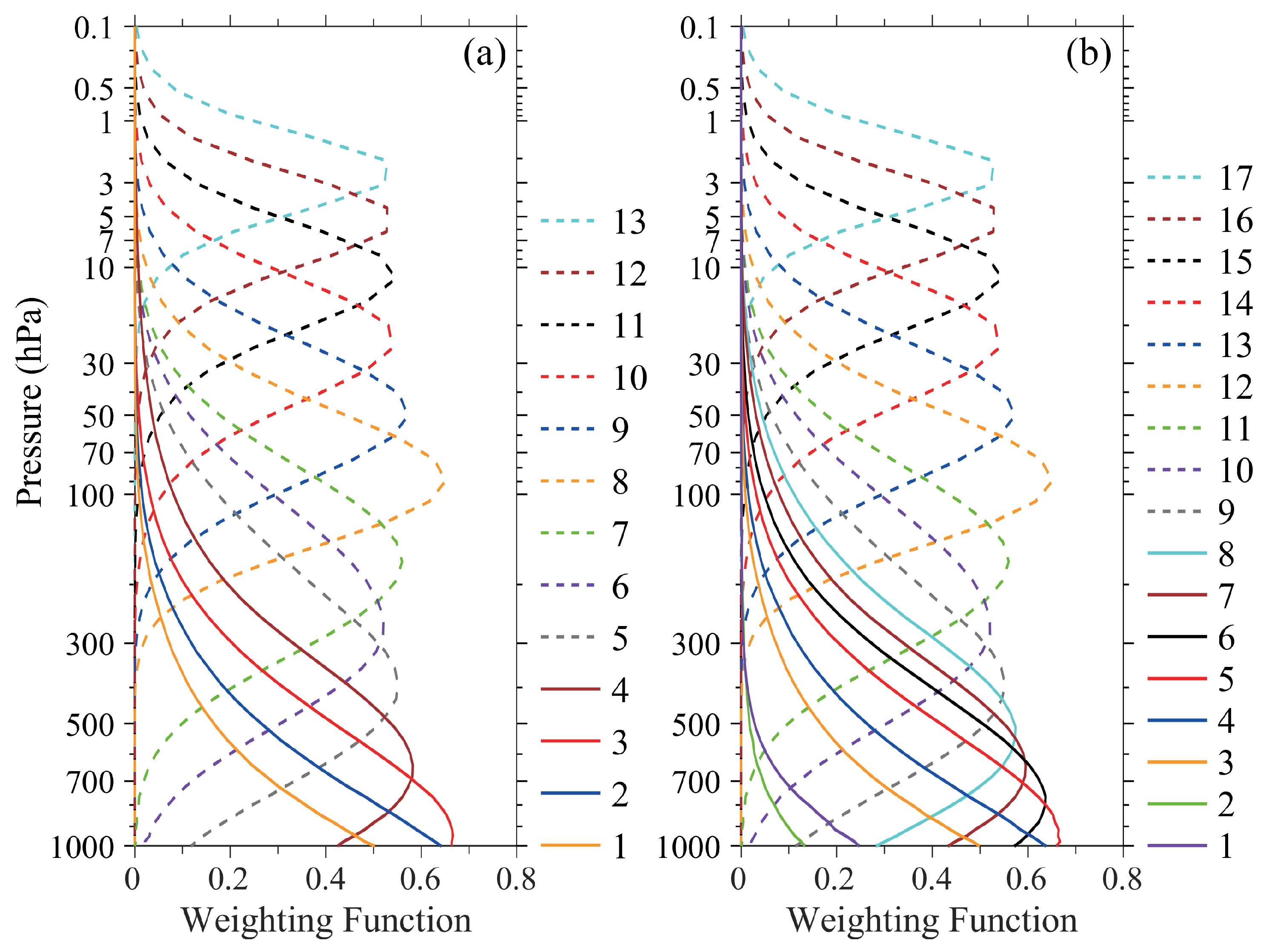
Table 1 shows a comparison of the channel frequencies between FY-3D MWTS-2 and FY-3E MWTS-3, and
Figure 1a,b show their weighting functions. MWTS-3 employs the same channels as MWTS-2 but includes four additional channels, namely, 23.8 GHz, 31.4 GHz, 53.246 ± 0.08 GHz and 53.948 ± 0.081 GHz, corresponding to channel 1, channel 2, channel 6 and channel 8, respectively. The peak values of the weighting functions of channel 1 and channel 2 are close to the ground, which was intended to strengthen the measurement of total water vapor. Channel 6 and channel 8 complement tropospheric temperature measurements at 700 hPa and 500 hPa, respectively. In addition, the sensitivity of MWTS-3 is greater than that of MWTS-2.
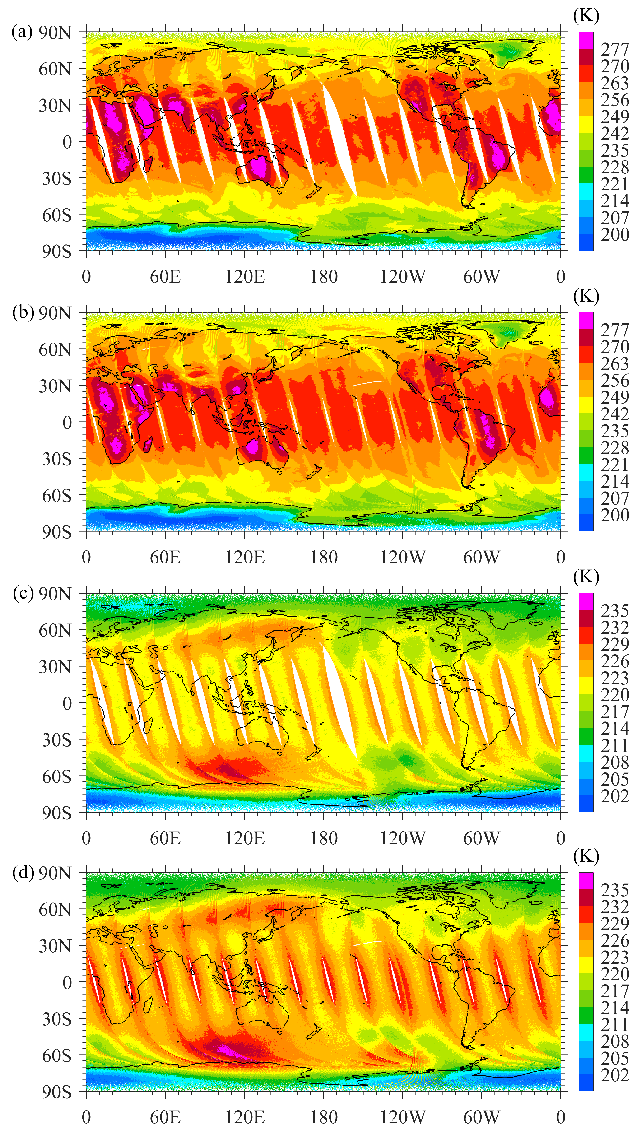
Figure 2a,b show the spatial distributions of the brightness temperature measured by MWTS-2 and MWTS-3 at approximately 950 hPa. MWTS-3 has a wider swath width and smaller gaps between orbits that are not covered by observations in the tropics. Except for MWTS-3 observing a larger area than MWTS-2 above 263 K in the tropical Pacific, the observations of the two instruments at 950 hPa are generally consistent. At 20 hPa, as shown in
Figure 2c,d, the brightness temperatures observed by MWTS-3 are approximately 2∼3 K higher than those observed by MWTS-2. Nevertheless, both MWTS-2 and MWTS-3 exhibit obvious striping noise, both in the near-ground channels and in the upper-level channels. The striping noises of the two microwave temperature sounders are extracted and quantitatively compared below.
3. Characteristics of the “” Distribution
In this paper, Radiative Transfer for TOVS version 13 (RTTOV 13; TOVS: TIROS Operational Vertical Sounder; TIROS: Television Infrared Observation Satellite) was used as the forward model to simulate the brightness temperatures of FY-3E MWTS-3 and FY-3D MWTS-2 based on data from the European Centre for Medium-Range Weather Forecasting (ECMWF) 5th-Generation Reanalysis (ERA-5) valid at 00:00 UTC, 06:00 UTC, 12:00 UTC and 18:00 UTC. The horizontal resolution of the reanalysis data was 0.25°, with 37 layers in the vertical direction. Because gridded data should be interpolated into the FOVs of the microwave temperature sounder before simulation, a nearest-neighbor interpolation was adopted to interpolate the temporal dimension of the reanalysis data, and a bilinear interpolation was used in the horizontal plane of each layer. A vertical interpolation was completed automatically by RTTOV 13 during the simulation.
“
” represent the difference between observed (O) brightness temperature and background field (B) brightness temperature (simulated by the radiation transfer model), which is also known as “first-guess departures”. In order to evaluate the error characteristics of observational data objectively in the absence of truth values, the model simulation errors are often assumed to be random. The mean value and standard deviation of “
” can be used to estimate the bias and observation error, respectively. In this paper, half a month of data covering the period from 24 September to 8 October 2021 were employed to calculate the mean value, standard deviation and interchannel correlation coefficients of “
”. To mitigate the effects of clouds and land surface emissivity, only clear-sky marine pixels were used in this study. The criteria for determining clear-sky pixels were that the total cloud water path was less than or equal to 0.02 kg·m
−2 [
12] and that the absolute value of “
” in any channel was less than three times the standard deviation. The land–sea mask of ERA-5 was used to identify marine pixels. This study focused on the Pacific Ocean, and therefore, the sampling area was delimited as a rectangle encompassing the range of 99°E∼78°W, 50°S∼50°N.
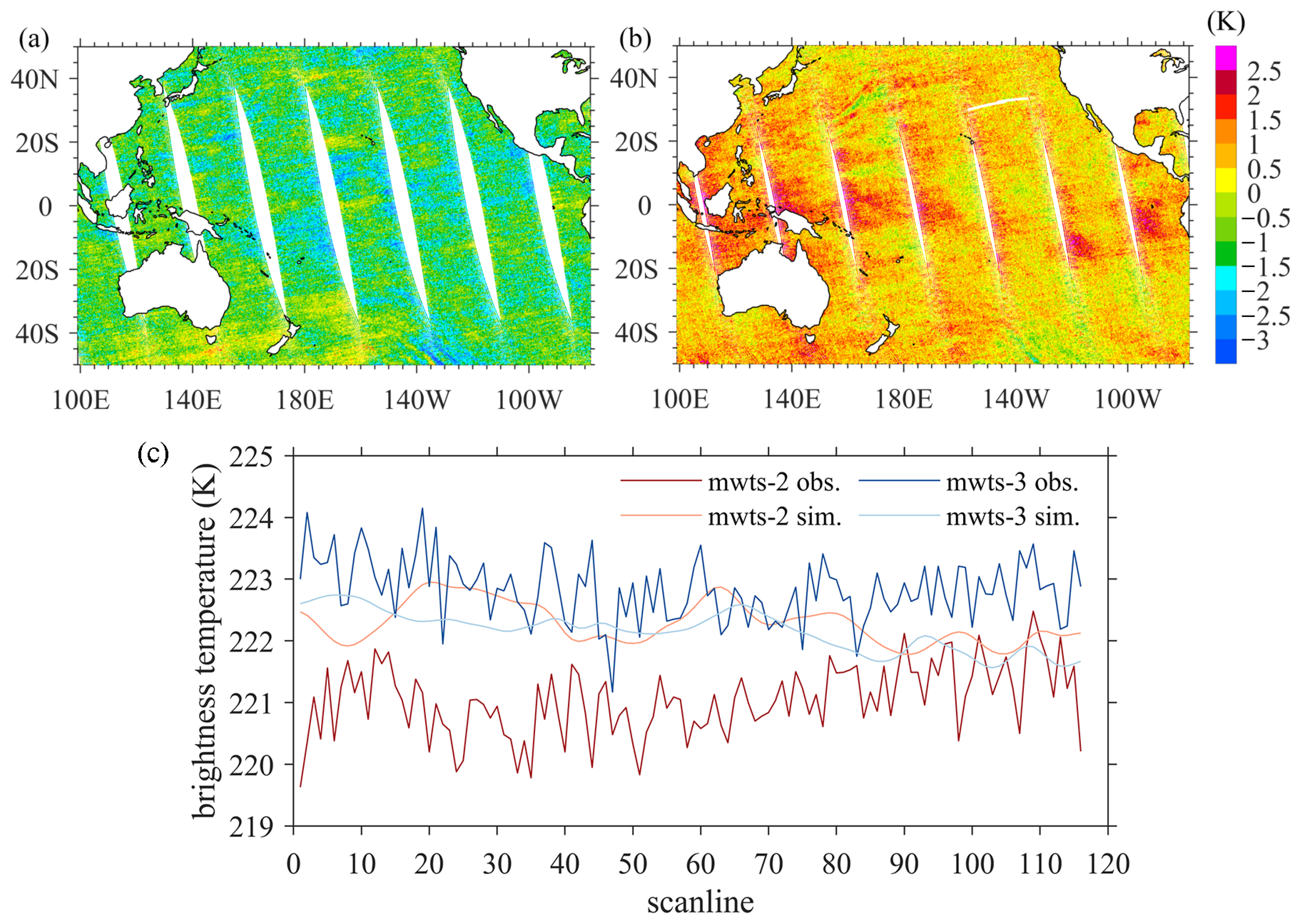
Figure 3 shows the spatial distribution of “
” in the 57.290334 ± 0.3222 ± 0.0480 GHz channel for MWTS-2 and MWTS-3 in the Pacific Ocean on 5 October 2021. MWTS-2 shows a negative bias with an average of approximately −1 K, while MWTS-3 shows a positive bias with an average of approximately 1 K. The difference between them is approximately 2 K, which is consistent with the difference in their observed brightness temperatures (2∼3 K) mentioned above. As shown in
Figure 3, striping noise appears clearly in the “
” distributions of both instruments.
4. Method of Extracting Striping Noise
In this study, the method that combines principal component analysis (PCA) with ensemble empirical mode decomposition (EEMD) [
13] was applied to extract and mitigate striping noise. PCA is a linear orthogonal transformation. By projecting the data onto several new coordinates, the original data are transformed into a group of linearly unrelated components, which are called the principal components. In order of the variance (from the maximum to the minimum) of the data in these new coordinates, the principal components are called the 1st, 2nd, 3rd PC mode, etc. The brightness temperature of
N scan lines in one channel of a microwave temperature sounder can be expressed as the matrix
:
where
M is the total number of FOVs on a scan line and
represents the brightness temperature of the
kth FOV on the
jth scan line. To obtain the PC modes, a matrix S is constructed as:
S is a real symmetric matrix and therefore must be diagonalizable:
where
is a diagonal matrix and
consists of
M linearly independent eigenvectors, i.e., the PC components.
After obtaining the principal components, the original data can be decomposed into principal components and the corresponding coefficients. In this study, we regarded the scanline as a 98-dimensional space vector and the along-track scaling factors as the PC coefficients. By Schmidt’s orthogonalization, E can be turned into an orthonormal basis (still written as E). According to the properties of orthogonal matrices, we can obtain:
Now the PC coefficients
U can be obtained by:
In this way, the brightness temperature matrix
A is decomposed into
E and
U:
where
E consists of the eigenvectors of the matrix
S;
represents the
ith eigenvector (i.e., the mode) of
S; and
represents the principal component coefficients corresponding to the
ith mode.
A can also be expressed as:
Then, the EEMD method was employed to filter the principal component coefficients. EEMD is an improved variation of the empirical mode decomposition (EMD) that takes advantage of the property that the mean value of white noise is 0. By repeatedly introducing evenly distributed white noise into the decomposition process and taking the resultant average of the corresponding components from different decompositions as the final result, the mode-aliasing problem in EMD is avoided [
14]. Let us consider any principal component coefficient
. EEMD is performed according to the following steps:
Add random white noise to P original sequences , where P is the set number of times that EMD is performed.
For each original sequence , apply a cubic spline to interpolate both the upper and the lower envelopes according to the peak and valley points of the sequence.
Find the mean values of the upper and lower envelopes and subtract them from to obtain the intermediate sequence.
Judge whether the intermediate sequence meets the following two conditions of an intrinsic mode function (IMF): (i) the difference between the number of extreme points and the number of zero-crossing points must be less than one, and (ii) the average of the upper envelope and lower envelope at any point must be zero. If so, the intermediate sequence is an IMF; otherwise, repeat steps (2) and (3) based on the intermediate sequence.
After obtaining the first IMF (IMF1), subtract it from
to obtain a new sequence,
. Repeat steps (2) to (4) based on
to obtain IMF2. By analogy, after
L iterations, the principal component coefficients are decomposed into
L IMFs and a residual sequence:
where
represents the
mth IMF of the original sequence
and
is the remainder.
Finally, express the ensemble mean of each IMF as:
Previous studies found that FY-3D MWTS-2 had strong striping noise, which was present not only in the first mode but also in the second and third modes as well [
9]. According to Zou’s research [
15], it is believed that the first three PC modes only embody the large-scale characteristics and the striping noise of the brightness temperature. Filtering those high-frequency noise in the coefficients of the first three modes will not affect weather signals. Therefore, the principal component coefficients of the first three modes were filtered by EEMD to eliminate the first three IMFs. After removing the striping noise, the brightness temperature matrix
can be expressed as:
A cubic spline interpolation requires certain boundary conditions to be established; thus, the errors at the boundaries are usually slightly larger than those in the middle. To eliminate the larger errors at the boundaries caused by the cubic spline interpolation, this study took 100 scan lines as steps to slide along the satellite track for sampling with a sample size of 300 scan lines (i.e., M = 300). After the PCA/EEMD processing, only the middle 100 scan lines were taken as the results for splicing. Finally, the striping noise was extracted by calculating the difference between and A. It should be noted that for the near-ground sounding channels, the brightness temperature gradient between sea and land was large. When the coastline was parallel to one of those scan lines, the strong brightness temperature gradient was similar to the striping noise characteristics, which led to excessive noise elimination in the ocean surface data. In order to alleviate this problem as much as possible, we added a correction step. According to the statistical results of striping noise of the two instruments, the striping noise with an absolute value greater than 1.0 K was considered as false striping noise and was not mitigated.
5. Comparative Analysis of Striping Noise between MWTS-3 and MWTS-2
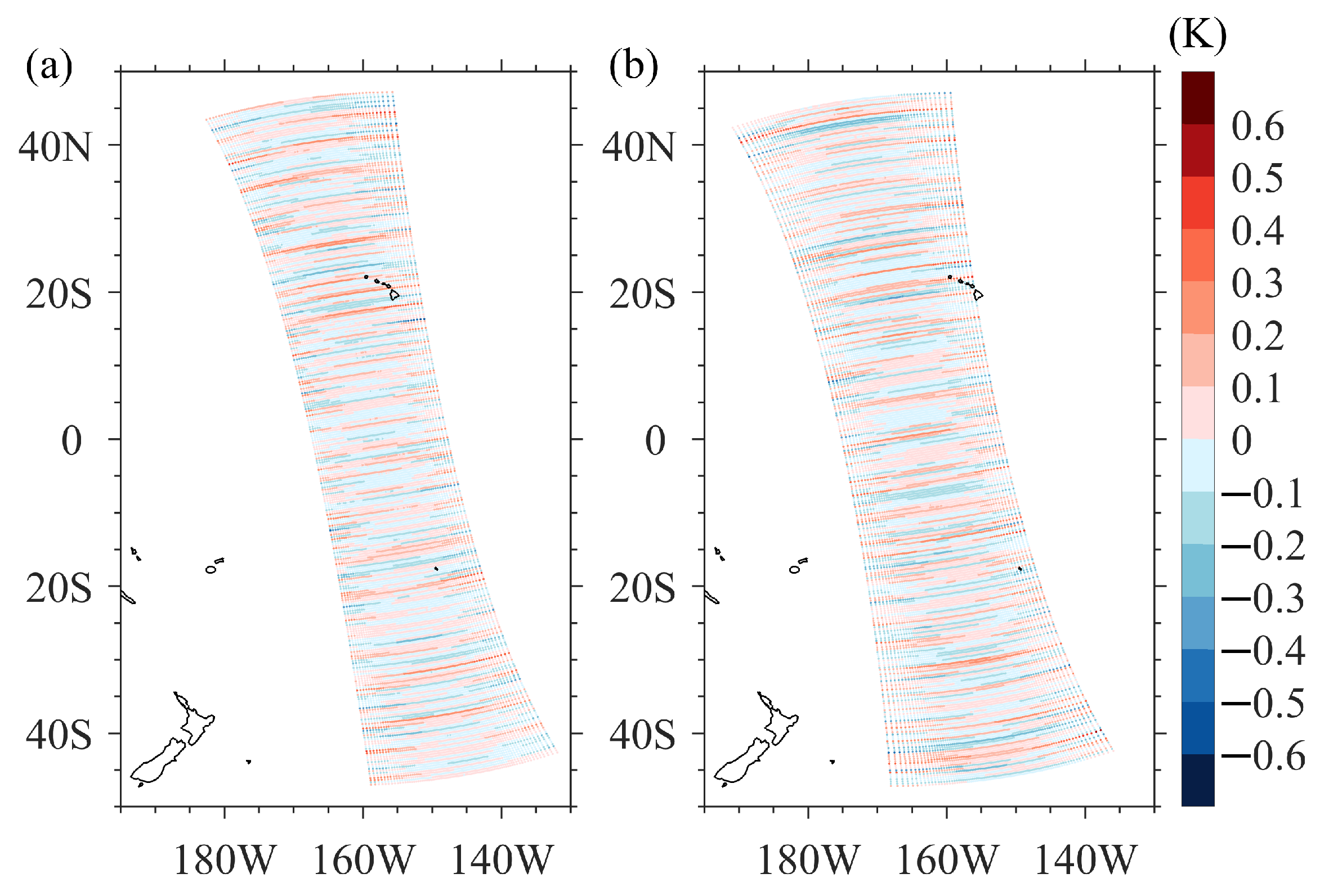
Both MWTS-2’s channel 6 and MWTS-3’s channel 10 have a central frequency of 54.94 GHz, with the weighting function peaking at approximately 300 hPa.
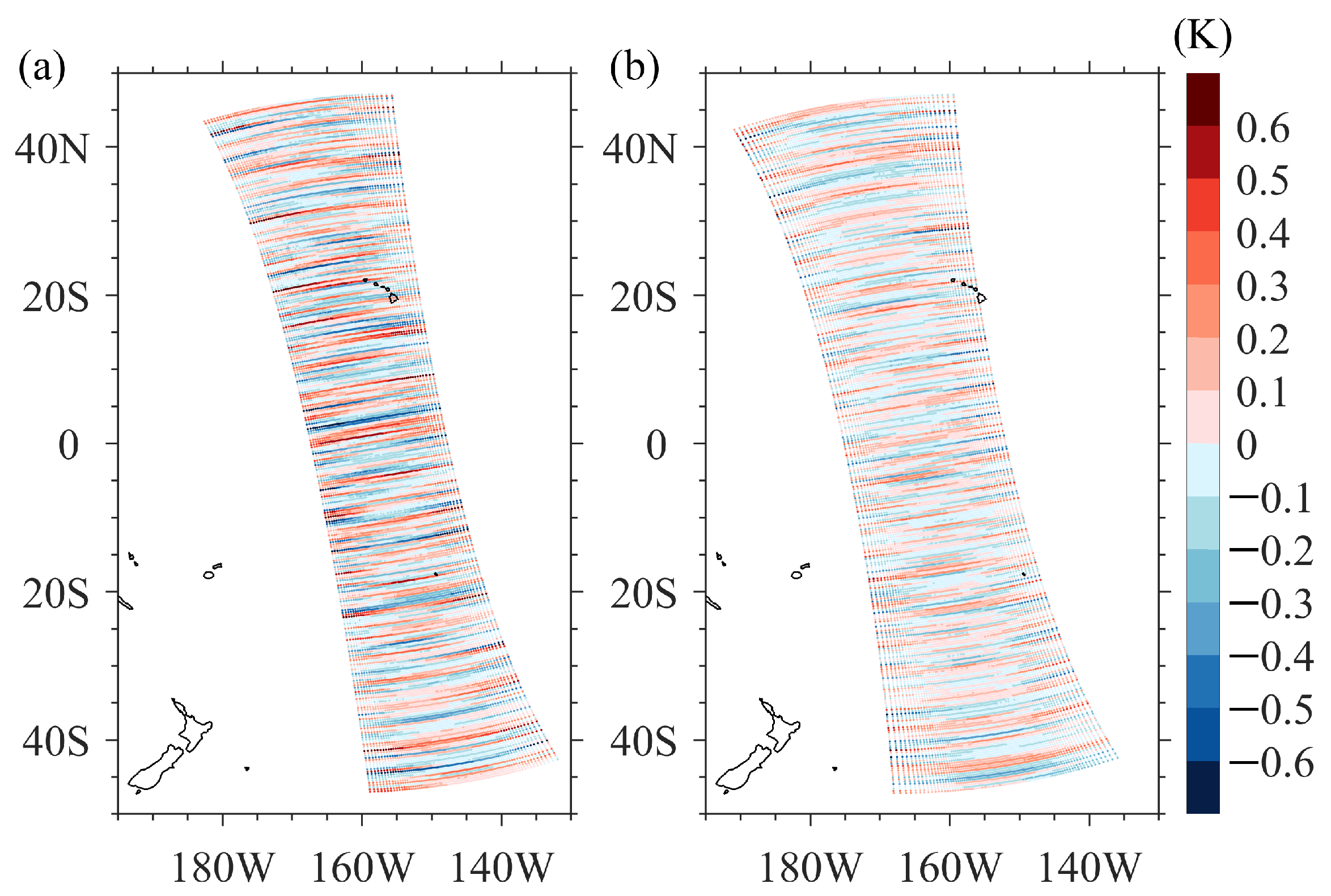
Figure 4 shows the spatial striping noise distributions of these two microwave temperature sounders at this frequency in the same region, namely, the Eastern Pacific, on 5 October 2021, each with 300 ascending scan lines. The striping noise intensities of the two were relatively similar: the mean value was approximately 0.1 K and the maximum was less than 0.4 K. However, the striping noise intensity varied significantly between MWTS-2’s channel 10 and MWTS-3’s channel 14.
Figure 5 shows that the striping noise of MWTS-2 was much stronger than that of MWTS-3.
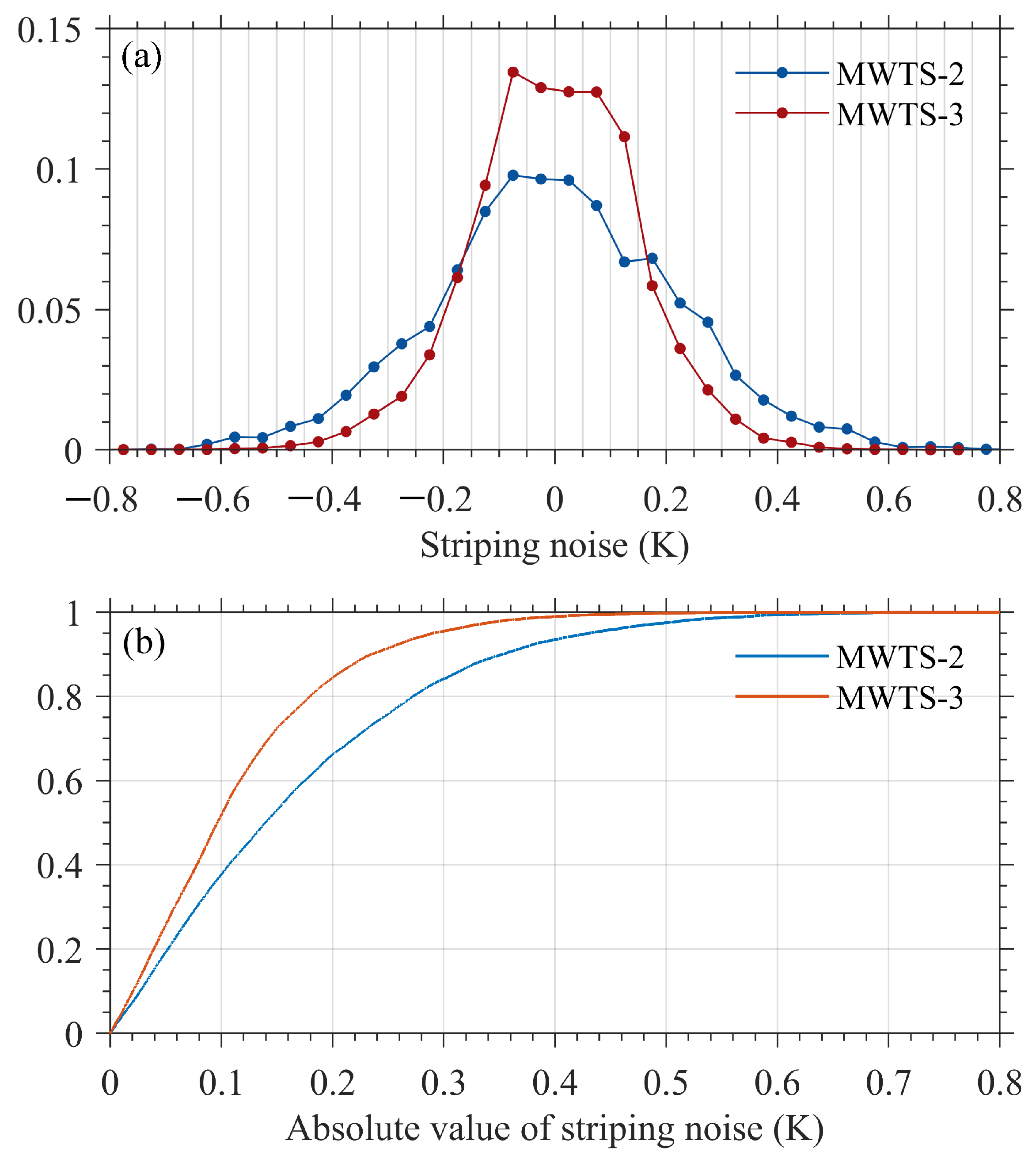
Figure 6a presents the normalized frequency for the striping noise of the 300 scan lines shown in
Figure 5a,b at an interval of 0.05 K. The striping noise of MWTS-3 was concentrated mainly between −0.15 K and +0.15 K, and the frequency within this range was much higher than that of MWTS-2. In contrast, the striping noise of MWTS-2 was more variable and appeared at higher frequencies beyond ±0.15 K than that of MWTS-3. According to the cumulative distribution of the absolute value of the striping noise (
Figure 6b), 70% of the striping noise of MWTS-3 fell within the range of ±0.15 K, while nearly half of that of MWTS-2 fell outside that range. As a result, at 57.290334 ± 0.3222 ± 0.0480 GHz, MWTS-2 had stronger striping noise overall.
The results plotted in
Figure 4 and
Figure 5 were extended over the entire Pacific Ocean, and the corresponding distributions of striping noise over the marine region of 99°E∼78°W and 50°S∼50°N shown in
Figure 7. The noise distribution in the Pacific was essentially uniform, and thus, the conclusion for 300 scan lines was applicable to the whole Pacific Ocean, indicating that the PCA/EEMD method for extracting striping noise was not affected by changes in brightness temperature.
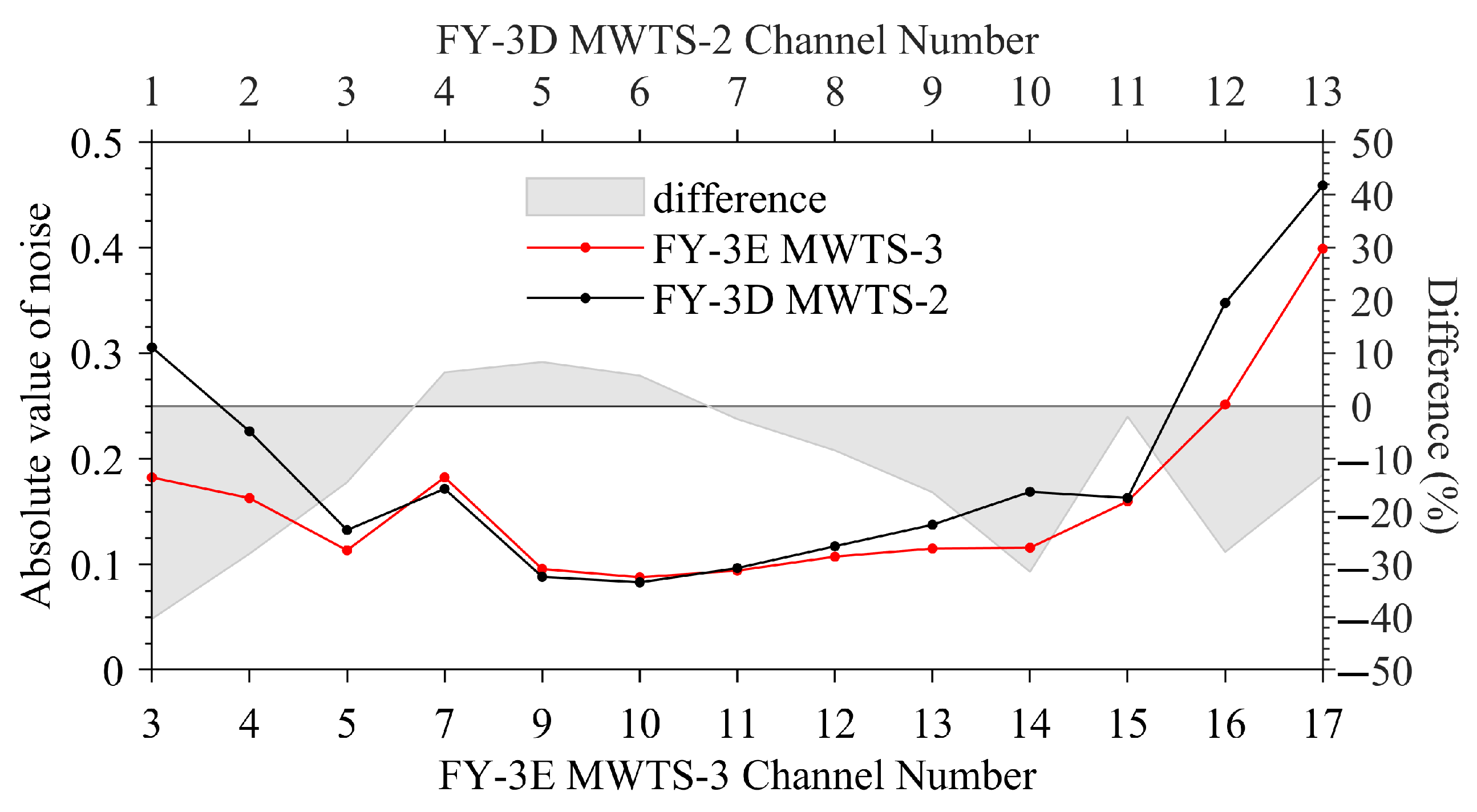
Figure 8 shows the average absolute value of the striping noise over 15 days (24 September to 8 October 2021) in the Pacific Ocean. The channels of the two microwave temperature sounders in
Figure 8 were matched according to the frequency, and the gray shaded area is the difference between them. The striping noises of channels 7 to 15 of MWTS-3 (corresponding to channels 4 to 11 of MWTS-2 at altitudes of 700 hPa to 10 hPa) were all less than 0.2 K. The striping noises of near-ground channels and high-frequency channels were relatively strong, with the largest noise appearing in MWTS-2’s channel 13, over 0.4 K. In general, the striping noise of MWTS-3 was weaker than that of MWTS-2. Although the striping noise of MWTS-3 in the middle four continuous channels (channels 7 through 10) was slightly stronger than that of the corresponding MWTS-2 channels, the maximum percentage increase was less than 9%, which was quite small compared with the intensity of the striping noise itself. The intensities of the striping noise of the other channels were all weakened to varying degrees, with a maximum reduction of approximately 42%. This finding shows that FY-3E MWTS-3 was improved with regard to the striping noise, which was well suppressed despite the increased number of FOVs. As mentioned above, the reduction of striping noises could be related to the improvement of the calibration. For a linear calibration, if the temperature of the cold and warm bodies as references are relatively stable, the noise along the track will be relatively small. This is only one possible explanation, and the definite cause of striping noise generation and reduction needs further exploration.
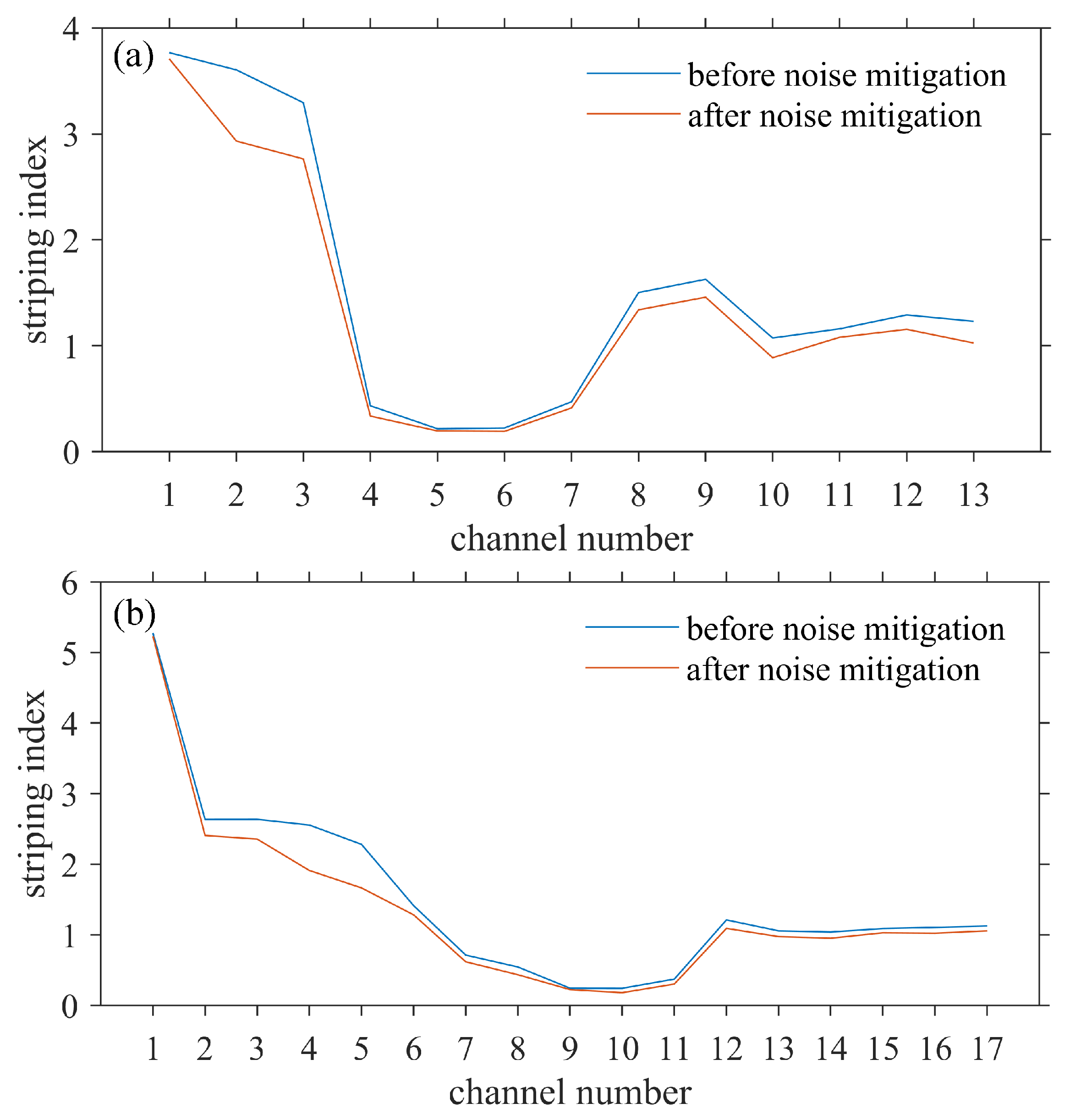
The striping index (SI) is defined as the ratio of along-track variance to cross-track variance of the observed brightness temperatures and is used to quantify the intensity of striping noise [
16,
17]. The calculated striping index is shown in
Figure 9. Since the Fengyun satellite has no pitch-over maneuver data, earth scene observation was used for calculating the index. Due to the influence of the limb darkening effect, weather system and latitudinal variation, the calculated striping index was not always greater than one as expected. It is worth noting that the striping index of both instruments decreased after noise mitigation, indicating that the striping noise was indeed suppressed.
6. Effect of Striping Noise on Interchannel Observation Error Correlations
Observation errors are assumed to be spatially independent in the theoretical derivation of the variational assimilation method. However, due to instrument calibration errors, cloud detection errors, radiative transfer model errors, striping noise and other reasons, the errors between the channels of microwave temperature sounders are always correlated [
18].
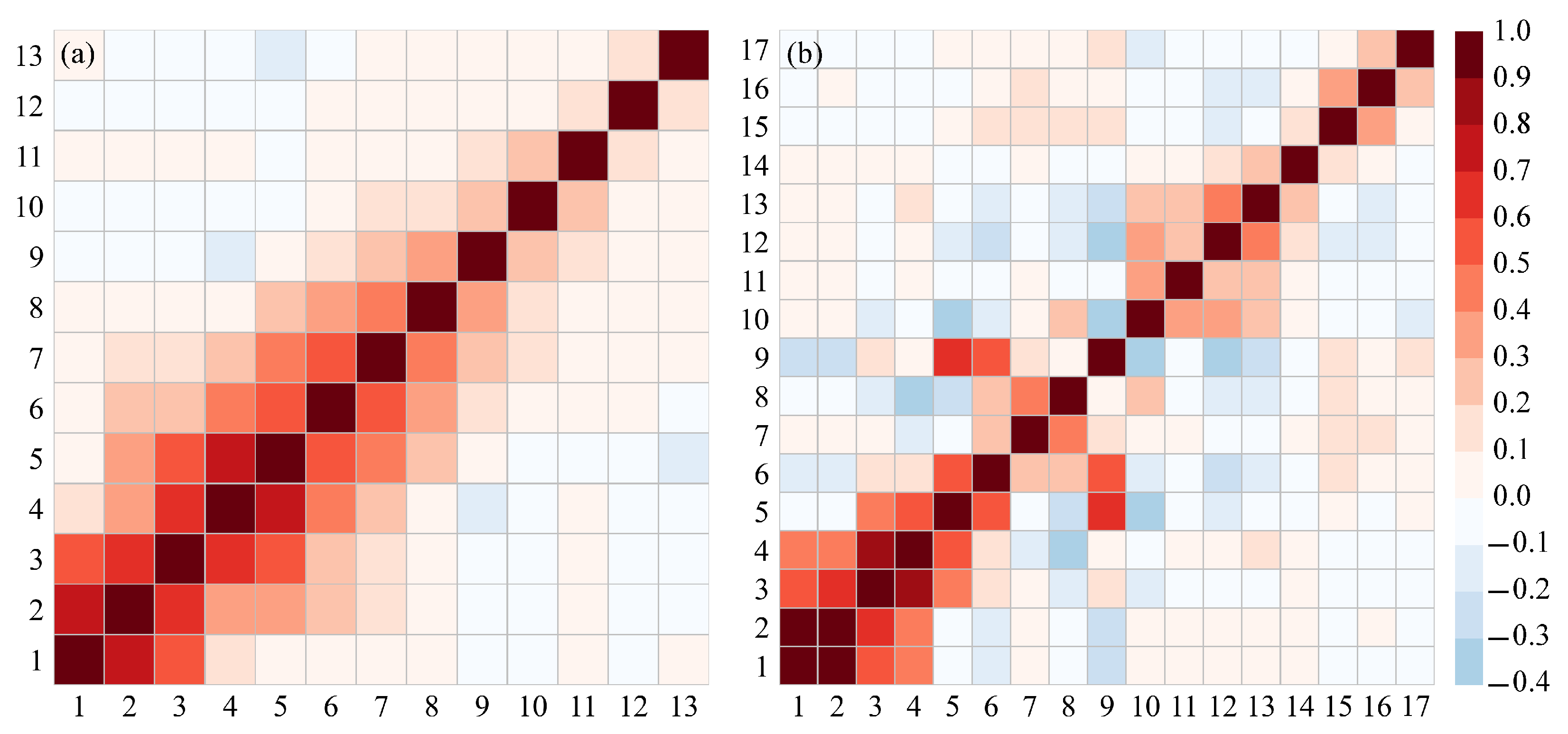
FY-3D MWTS-2 showed significant interchannel correlations between observation errors, mainly between the errors in channels 1 through 10. As shown in
Figure 10a, the correlation coefficients between channels were almost all positive and exhibited a pattern of gradually decreasing from the diagonal outward. For MWTS-3, continuous and significant positive correlations appeared only among the low-level channels (channels 1 through 4), while the correlations between the other channels were not obvious. More negative correlation coefficients were observed for MWTS-3, which was different from MWTS-2, whose 10 adjacent channels were positively correlated with each other. Overall, the interchannel error correlations of MWTS-3 were significantly weaker than those of MWTS-2. It is also noted that the correlation coefficients of some channels were negative. The channels with obvious negative correlations need further explorations to determine whether it was caused by the instrument itself or by the weather system, so as to give proper consideration to the actual application of the data.
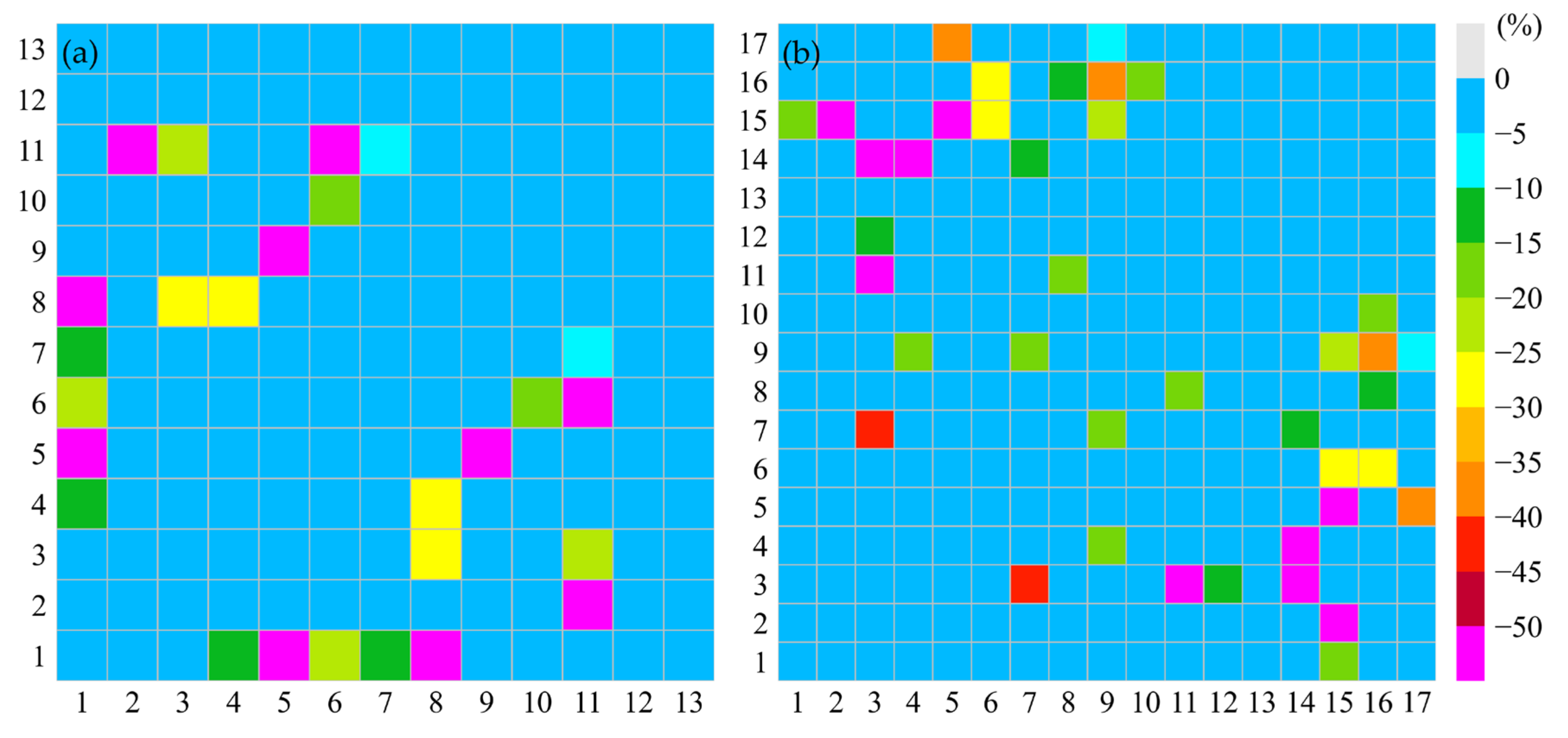
To verify the influence of the striping noise on these interchannel error correlations and to quantitatively evaluate the contribution of the striping noise to the correlation coefficients,
Figure 11 shows the changes in the absolute values of the correlation coefficients after noise mitigation. As shown by
Figure 11, the striping noise contributed more to the correlations of the weak-correlated couples of channels. A reduction of the correlation coefficients between the weak-correlated channels could reach up to 50%. This may indicate that the main contribution of the strong-correlated couples of channels was the incapableness of RTM to simulate some deep weather systems. However, for some couples of channels, mainly the nonadjacent couples, striping noise was the main cause for the correlations and the contribution could reach over 93% for the maximum. It was reasonable because the more the channels were spaced, the more different their sounding levels were, and thus the striping noise became the main reason for their correlations.
7. Effect of Striping Noise on the Standard Deviation of “”
Among the effects of the striping noise on “
” characteristics, the variation in the standard deviation is of most concern.
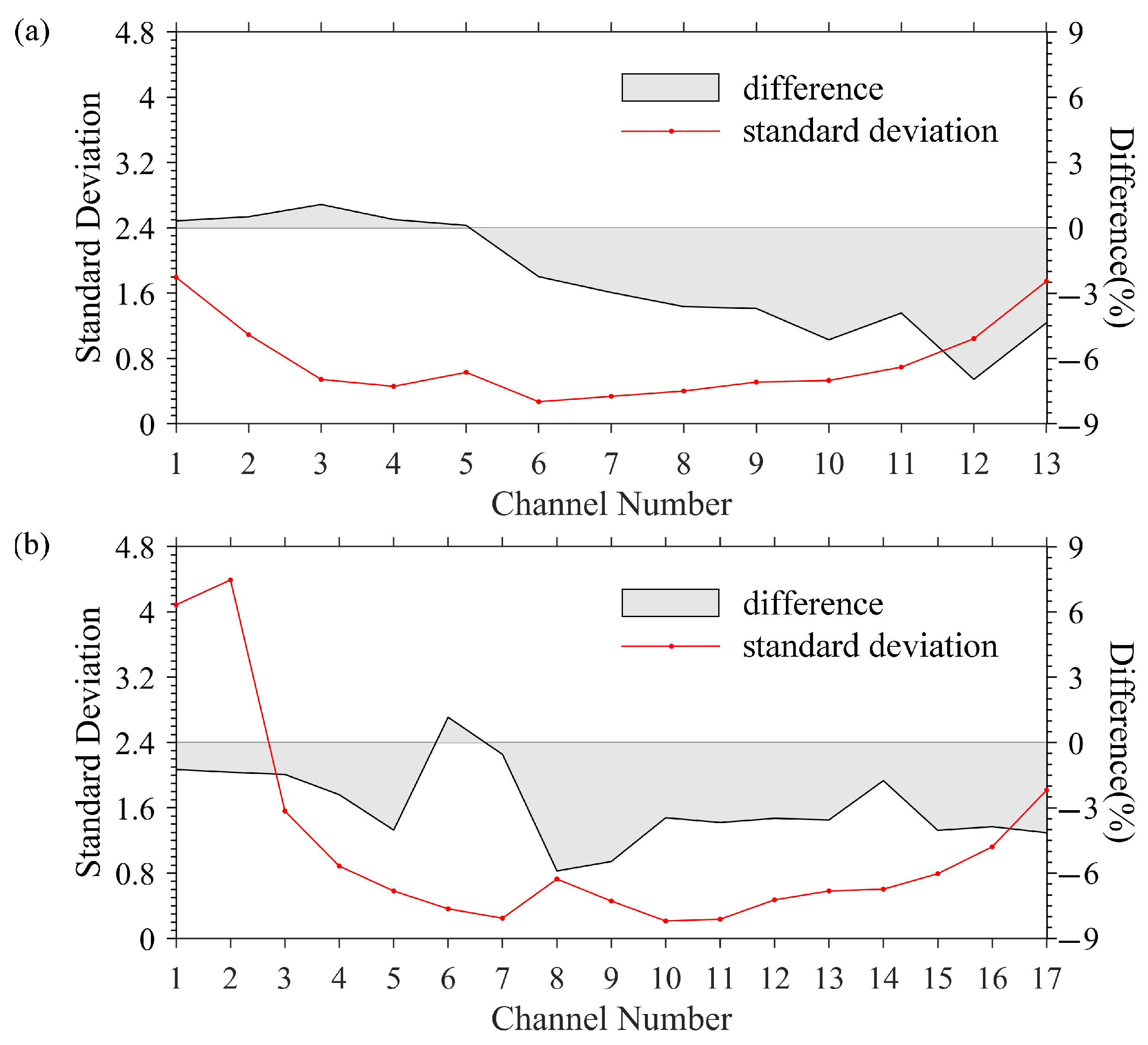
Figure 12 shows the change in the “
” standard deviation before and after noise mitigation; the red dotted curves represent the original “
” standard deviation of each channel, and the gray shaded areas represent the changes. The near-ground sounding channels, especially channels 1 and 2 of MWTS-3, had larger standard deviations. This was because these channels were more sensitive to weather systems, which could result in errors in “
” if the simulations were not able to capture the small-scale weather patterns. It can be seen that the observation errors of most channels of the MWTS-3 were reduced after noise mitigation. The most obvious error reduction was in channel 17, with the observation error reduced by nearly 0.1 K. The observation errors of other channels were generally reduced by about 5%, and only the observation error of channel 6 increased slightly. For the FY-3D MWTS-2, the observation errors of those near-ground channels also increased slightly but only by 1%. The observation errors of other channels were all decreased, and the maximum reduction of channel 12 could reach 7%.
8. Conclusions
In this paper, we evaluated the striping noise of FY-3E MWTS-3 and its effect on the interchannel error correlations and the “” standard deviation by comparing the MWTS-3 striping noise characteristics with those of MWTS-2 onboard FY-3D, an in-orbit service satellite. The main conclusions are as follows:
First, MWTS-3 had weaker striping noise, particularly in channels 3, 14 and 16. In channels 7 through 13, the striping noise intensity was comparable to that of the MWTS-2 channels.
Second, the error correlations between the MWTS-3 channels were weaker than those between the MWTS-2 channels, and the striping noise was one of the contributors to the interchannel correlations. The correlation coefficients between the strong-correlated channels did not significantly decrease after noise mitigation, but the striping noise was a significant contributor to the error correlations between the nonadjacent channels.
In addition, the “” standard deviations reduced in the mid- and high-level sounding channels of both instruments but slightly increased in several low-level sounding channels of MWTS-2 after noise mitigation.
The above results demonstrate that MWTS-2 was greatly affected by striping noise, and it is suggested that such noise be removed before data assimilation, whereas MWTS-3 was less affected.
