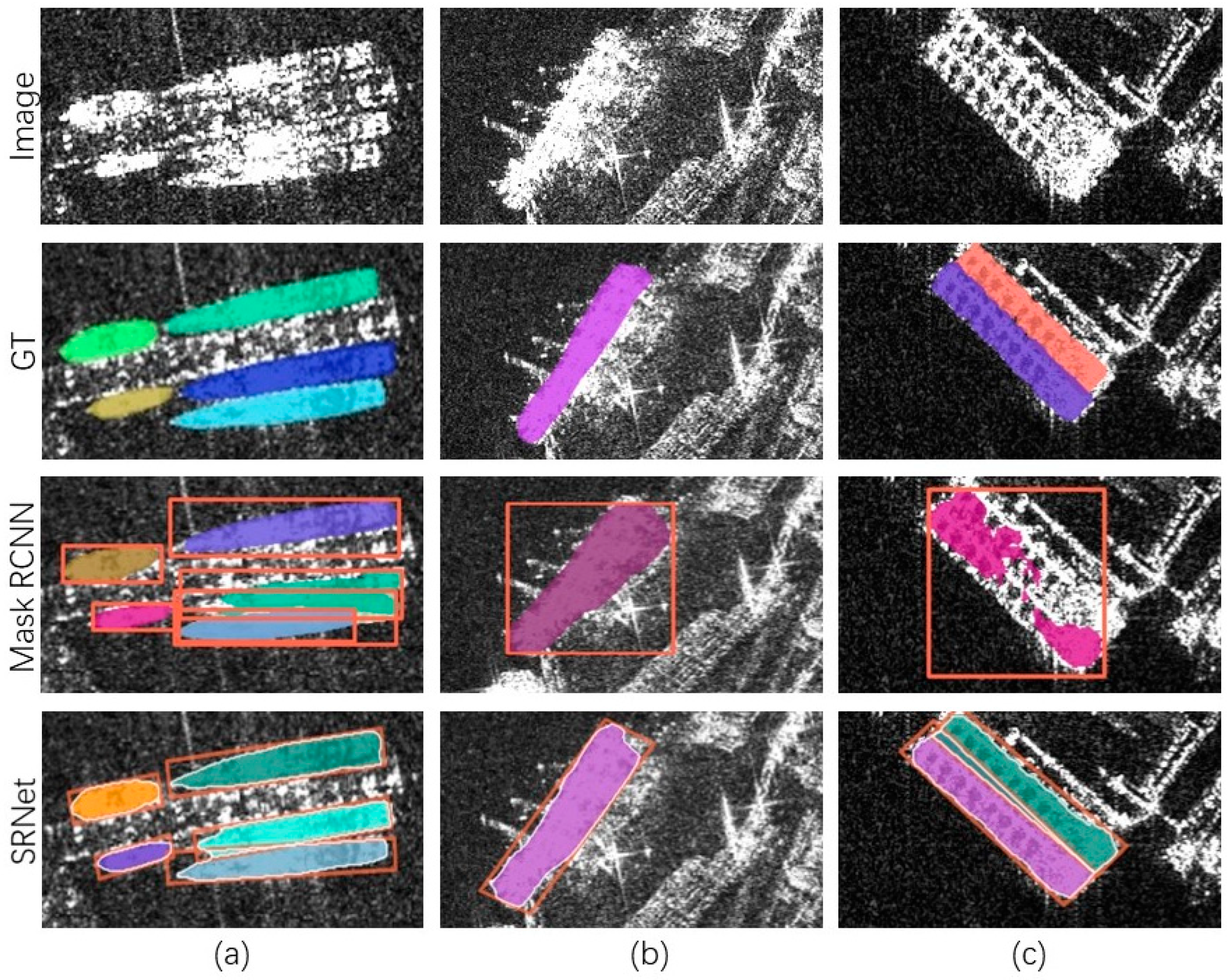
Figure 1.
Visual comparison between the instance masks from the HB-Box-based Mask RCNN and from our RB-Box-based SRNet. (a) The scene of the densely packed ships. (b) The scene of the ship berthing in a dock. (c) The scene of parallel ships.
Figure 1.
Visual comparison between the instance masks from the HB-Box-based Mask RCNN and from our RB-Box-based SRNet. (a) The scene of the densely packed ships. (b) The scene of the ship berthing in a dock. (c) The scene of parallel ships.
Figure 2.
Overview of the proposed SRNet, consisting of a feature extraction procedure, a detection procedure, and a segmentation procedure. In the feature extraction procedure, the FPN takes feature maps C3, C4, and C5 extracted by the backbone as inputs and then outputs semantic feature maps P3–P7. In the detection procedure, these semantic feature maps are first transmitted to the DAM to produce the classification feature maps and regression feature maps. Then the DetHead takes the outputs of DAM as inputs to output the RB-Boxes and their classification scores. The segmentation procedure takes the RB-Boxes and the semantic feature maps as inputs and then outputs the final instance masks.
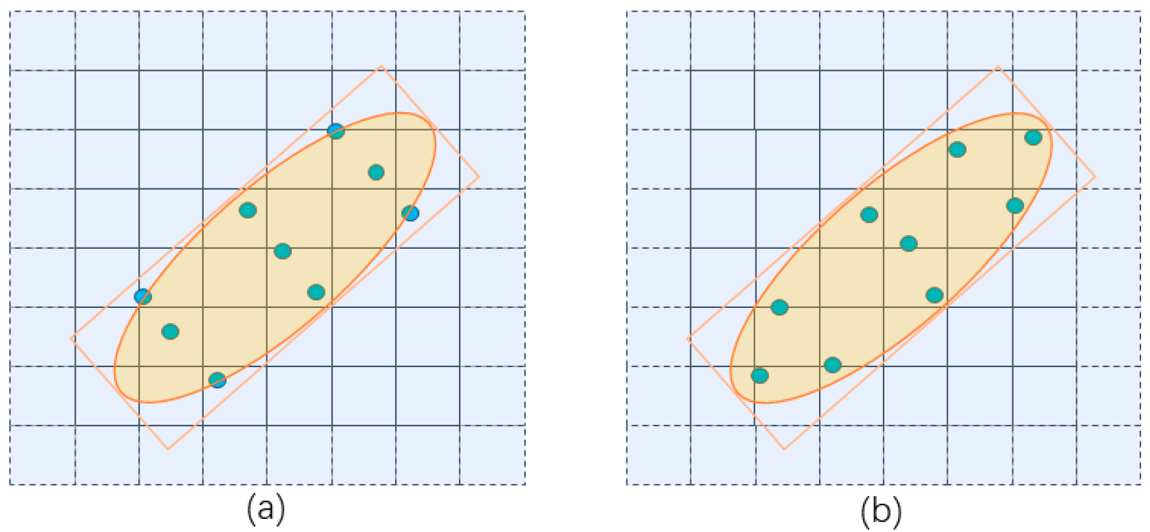
Figure 3.
The two sets of sampling locations (blue points). The sampling locations of the RAConv (a). The sampling locations of the CAConv (b). The orange RB-Boxes indicate the kernels. The yellow ellipses circle the ship areas.
Figure 3.
The two sets of sampling locations (blue points). The sampling locations of the RAConv (a). The sampling locations of the CAConv (b). The orange RB-Boxes indicate the kernels. The yellow ellipses circle the ship areas.
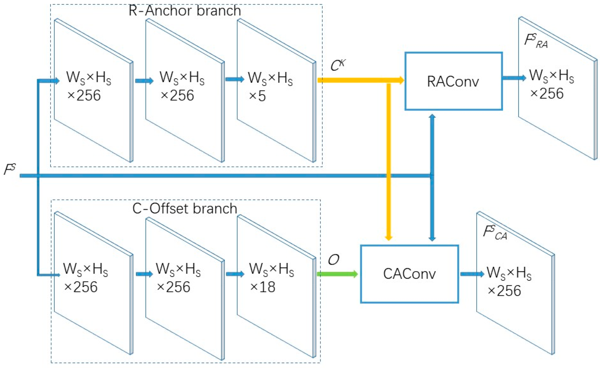
Figure 4.
Overview of the DAM, which consists of two convolutional branches (R-Anchor branch and C-Offset branch) and two alignment convolutions (RAConv and CAConv). With the feature map () of scale () as input, the R-Anchor branch produces the kernel coordinates (), and the C-Offset branch produces the sampling offsets (). The represents a feature map with the width of , the height of , and the channel of extracted by convolution. With the kernel coordinates () and the sampling offsets (), the RAConv and CAConv produce the regression feature map () and classification feature map (), respectively.
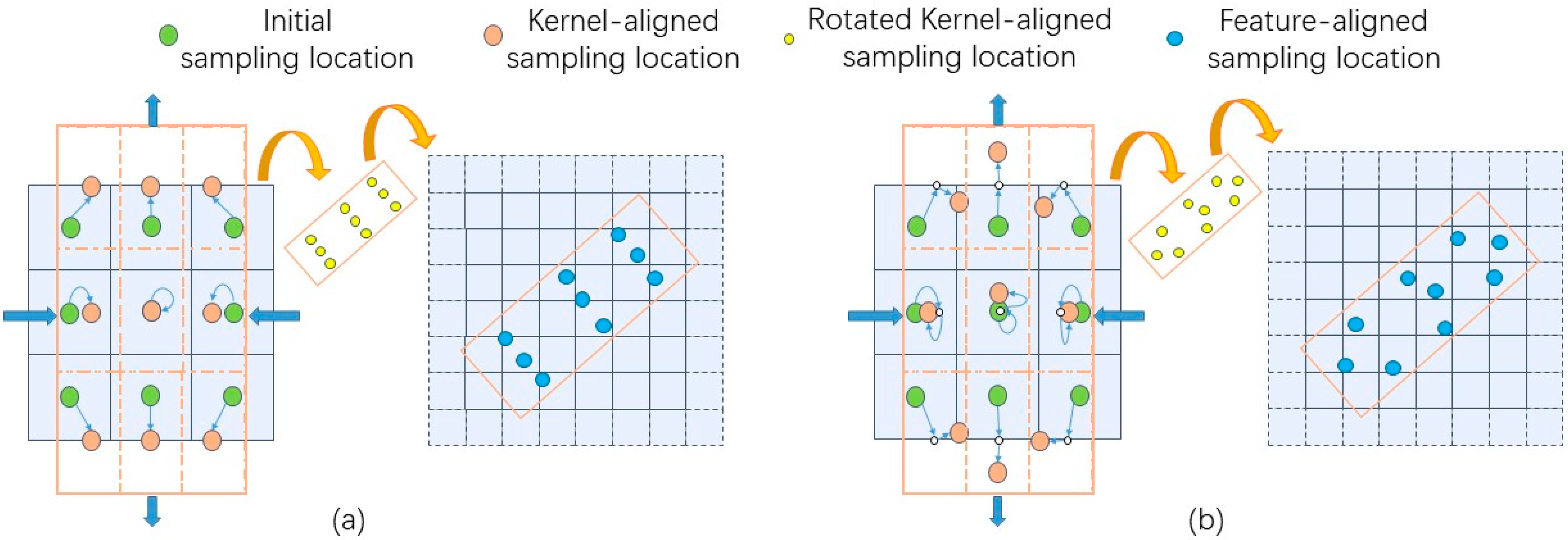
Figure 5.
The calculation pipeline of the sampling locations for the RAConv (a) and the CAConv (b). The left figures in (a,b) demonstrate the process of the initial sampling locations moving along the blue arrows to the kernel-aligned sampling locations. With the rotation (middle figure in (a,b)) and translation (right figure in (a,b)) the feature-aligned sampling locations on the feature map coordinate system are obtained.
Figure 6.
Overviews of the DetHead (a) and the MaskHead (b). In (a), and are input into two different three-layer convolutional networks to predict the RB-Boxes and their classification scores. Then the rotated NMS algorithm produces the final results. In (b), with the as input, the feature map, , output from a three-layer convolutional network and the RB-Boxes is used to produce the final instance masks by the RB-Box instance mask prediction.
Figure 7.
The pipeline of the RB-Box instance mask prediction: (a) indicates the feature sampling process, and (b) indicates the mask sampling process. In (a), the feature values in the RB-Box are computed with their nearest feature values in . Then a standard 1 × 1 convolution, Conv, is used to produce the instance mask, , in the RB-Box. In (b), the instance mask values in instance mask are computed with their nearest mask values in the RB-Box instance mask, . Then, the is enlarged times to obtain the instance mask in the original SAR image.
Figure 8.
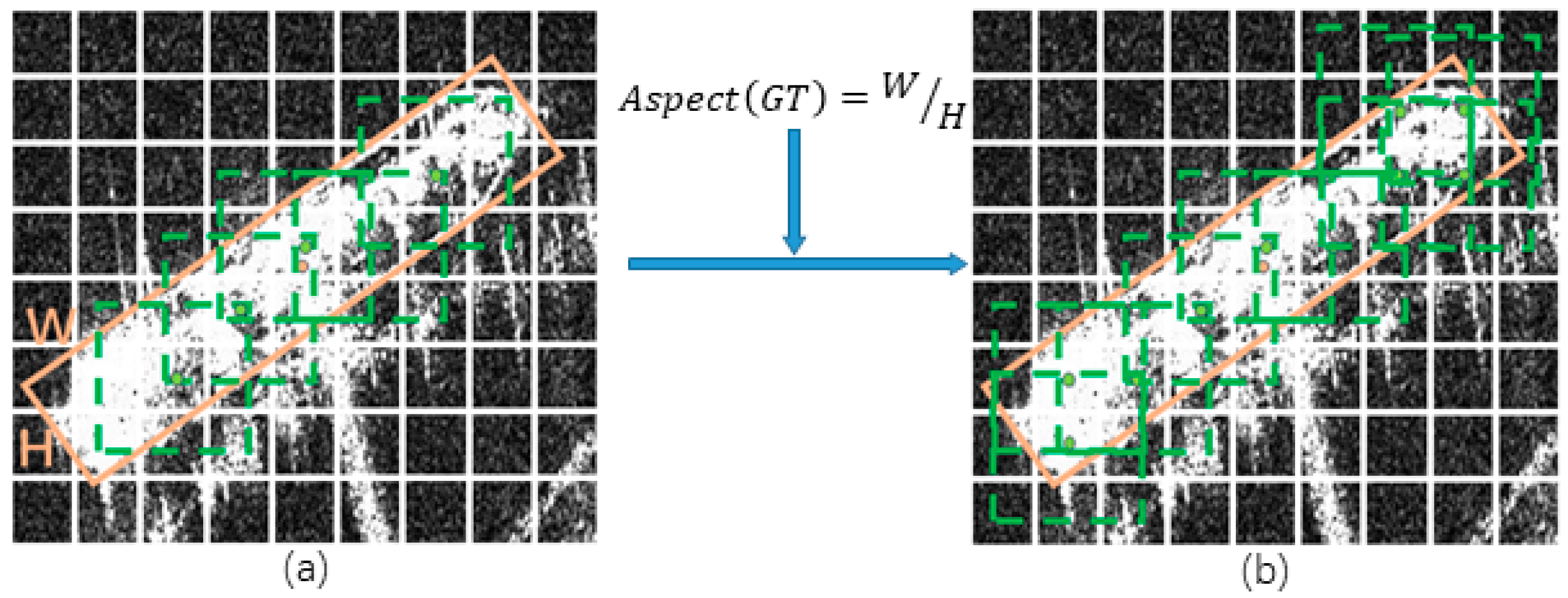
Comparison illustration of two IoU thresholds. (a) The positive sample allocation results of the ATSS. (b) The positive sample allocation results of the new adaptive IoU threshold with the aspect ratio. The green square boxes represent positive samples, and the green points represent their center points.
Figure 9.
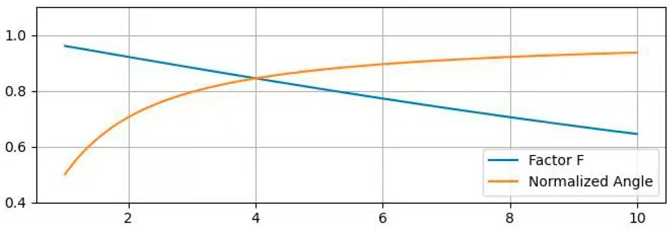
Illustration of the factor and the normalized angle with . The horizontal axis represents the aspect ratio. The vertical axis represents the value of the factor and the normalized angle.
Figure 9.
Illustration of the factor and the normalized angle with . The horizontal axis represents the aspect ratio. The vertical axis represents the value of the factor and the normalized angle.
Figure 10.
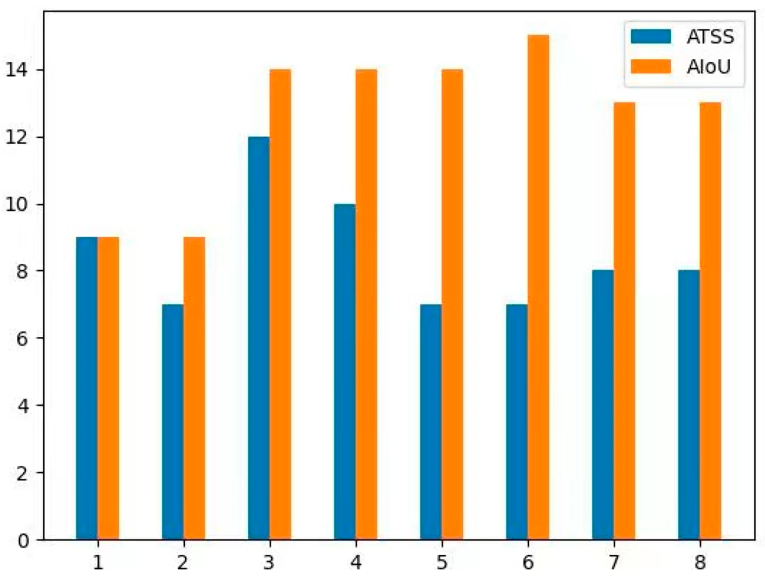
Illustration of the number of positive samples allocated by the ATSS and the AIoU. The horizontal axis represents the aspect ratio. The vertical axis represents the number of positive samples.
Figure 10.
Illustration of the number of positive samples allocated by the ATSS and the AIoU. The horizontal axis represents the aspect ratio. The vertical axis represents the number of positive samples.
Figure 11.
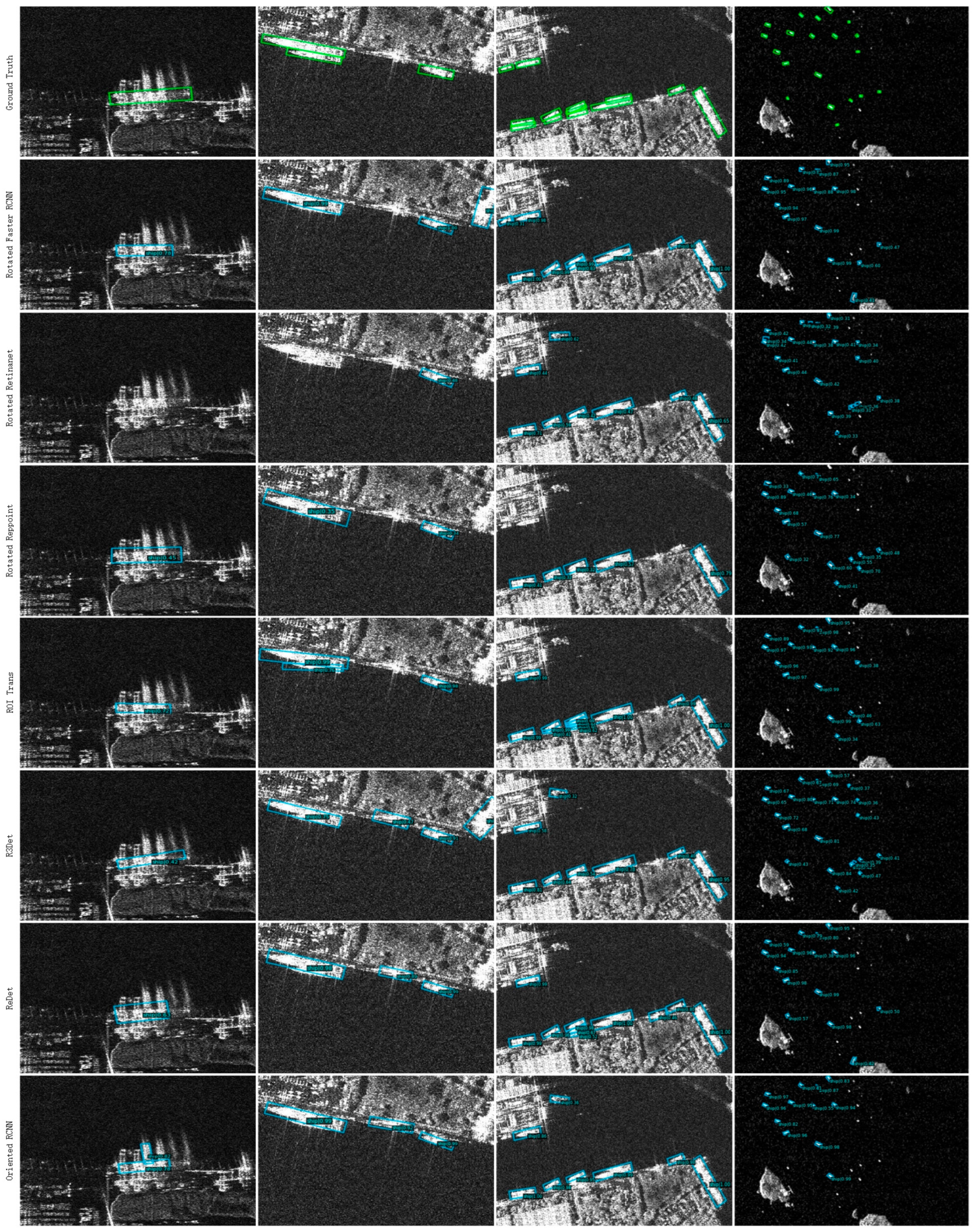
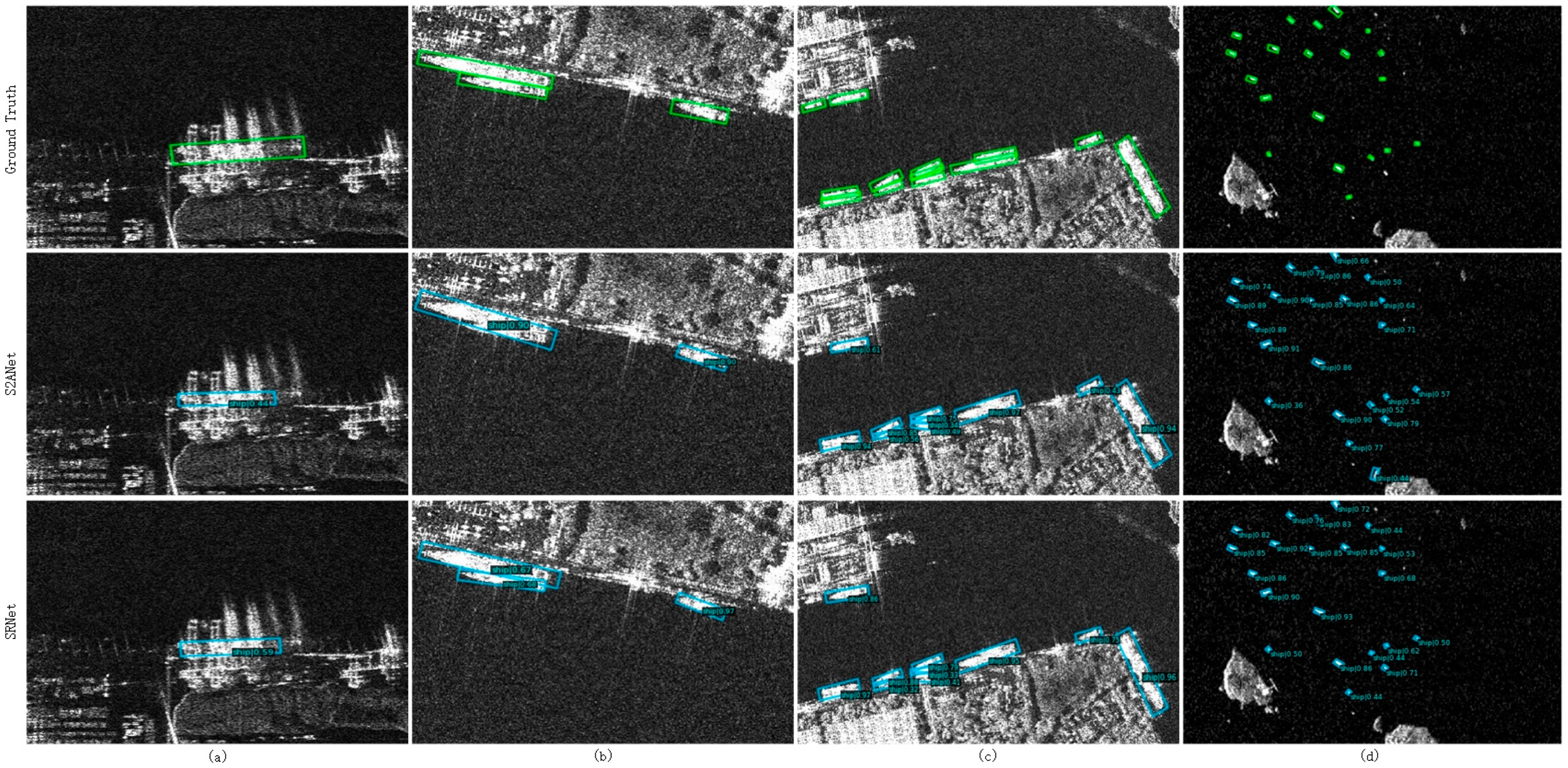
Four visualization illustration images of different comparison networks for rotated object detection on the SSDD dataset. (a) The scene of a single ship berthing in a dock. (b) The scene of parallel ships berthing in a dock. (c) The scene of multiple parallel ships berthing in a dock. (d) The scene of multiple ships sailing in the water region.
Figure 12.
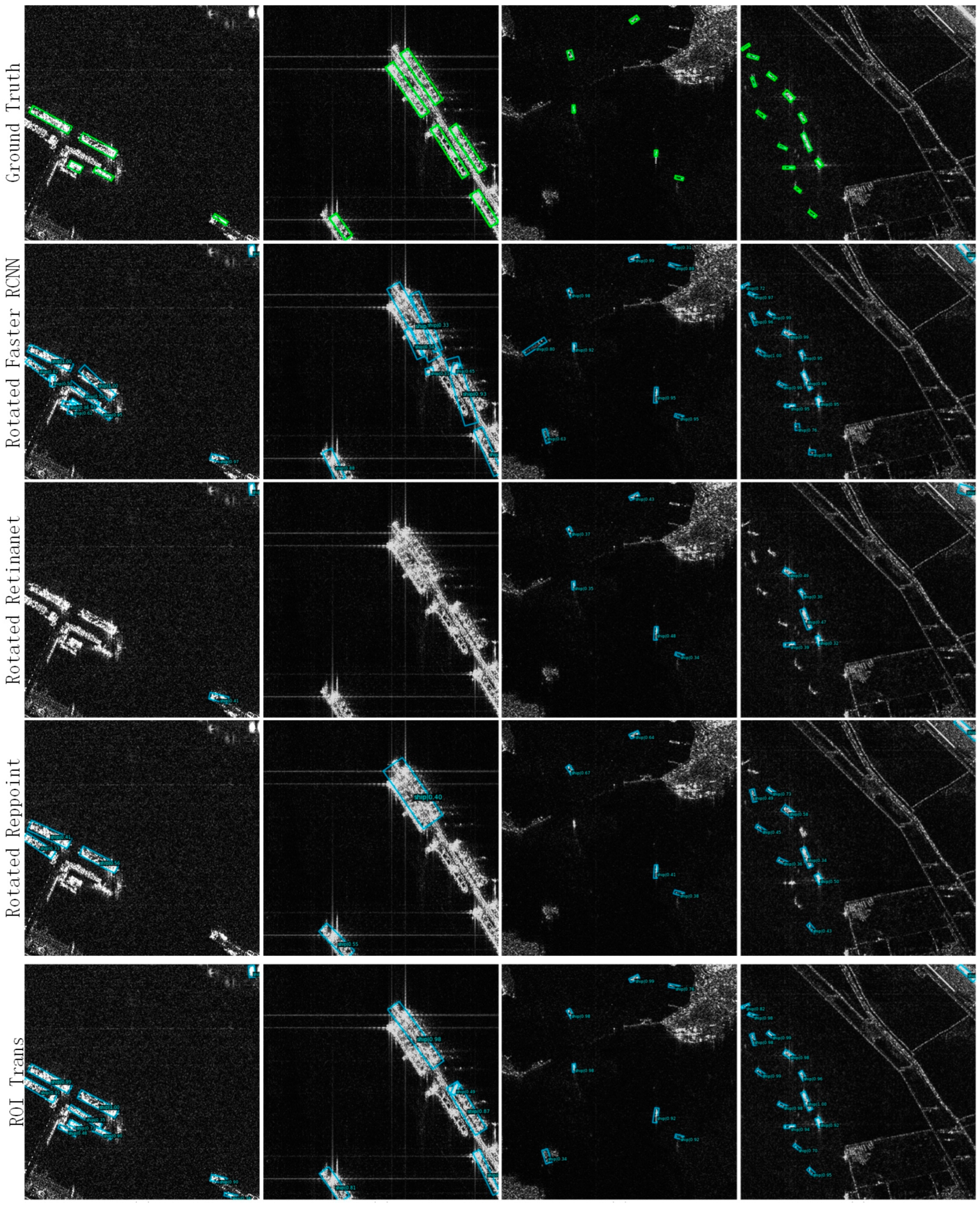
Four visualization illustration images of different comparison networks for rotated object detection on the RSDD dataset. (a) The scene of the ships berthing on one side of a dock. (b) The scene of the ships berthing on both sides of a dock. (c,d) The scene of ships sailing in the water region.
Figure 13.
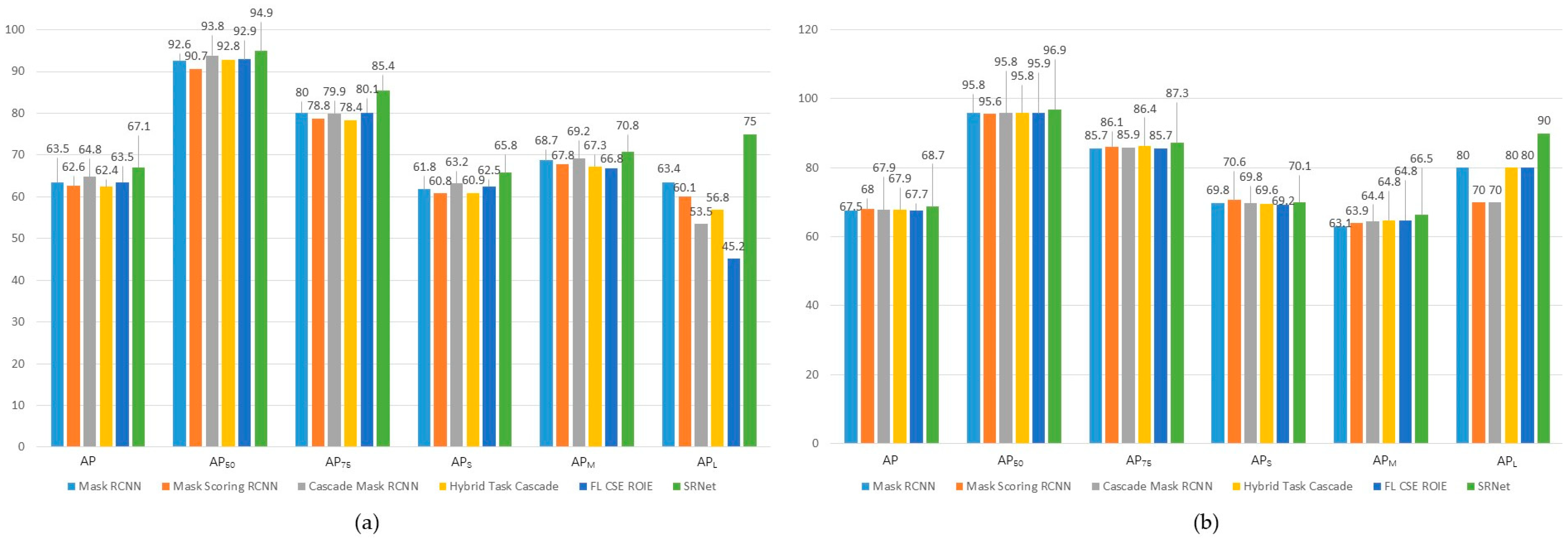
The histograms of instance-segmentation performance on the SSDD dataset (a) and the Instance-RSDD dataset (b).
Figure 13.
The histograms of instance-segmentation performance on the SSDD dataset (a) and the Instance-RSDD dataset (b).
Figure 14.
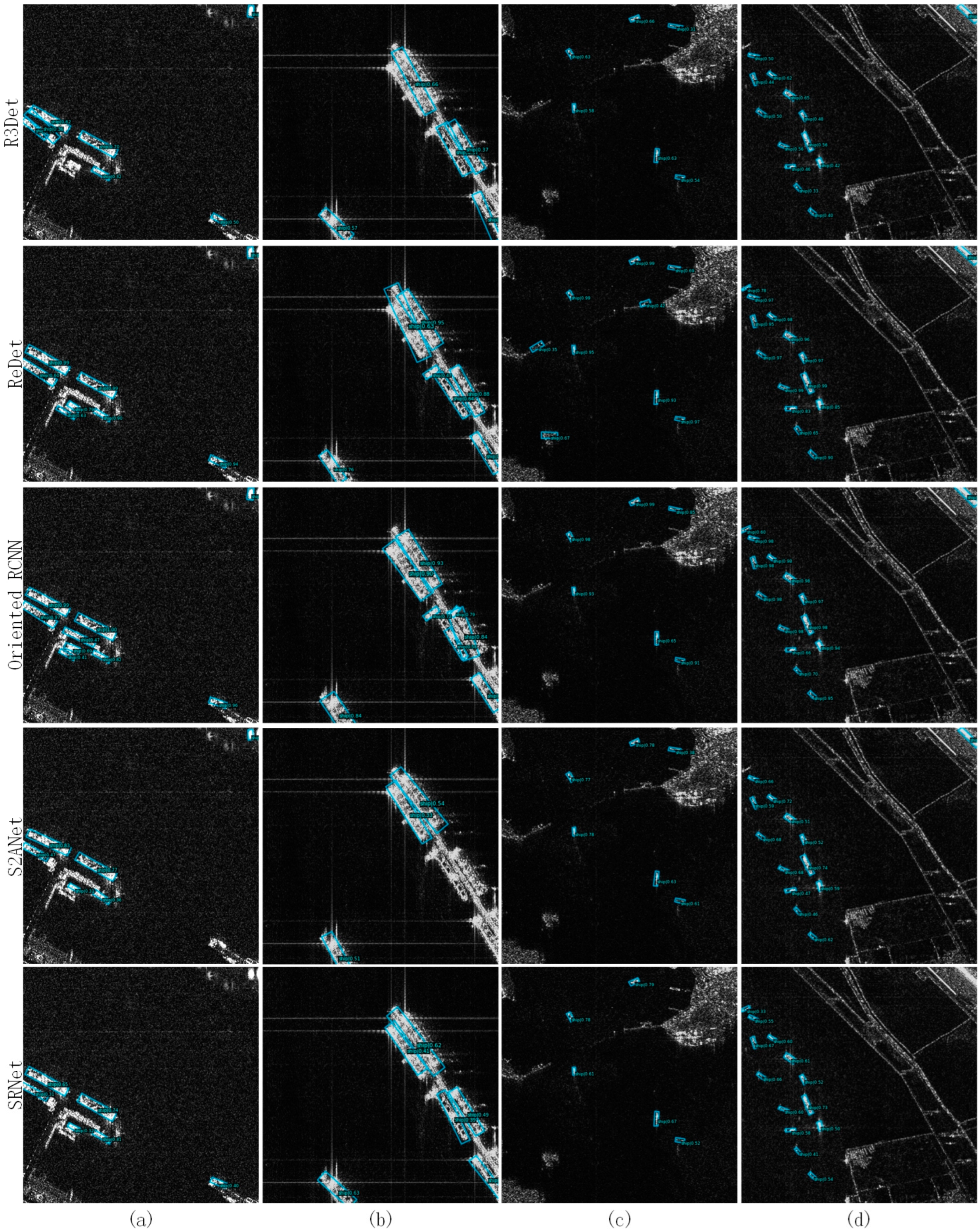
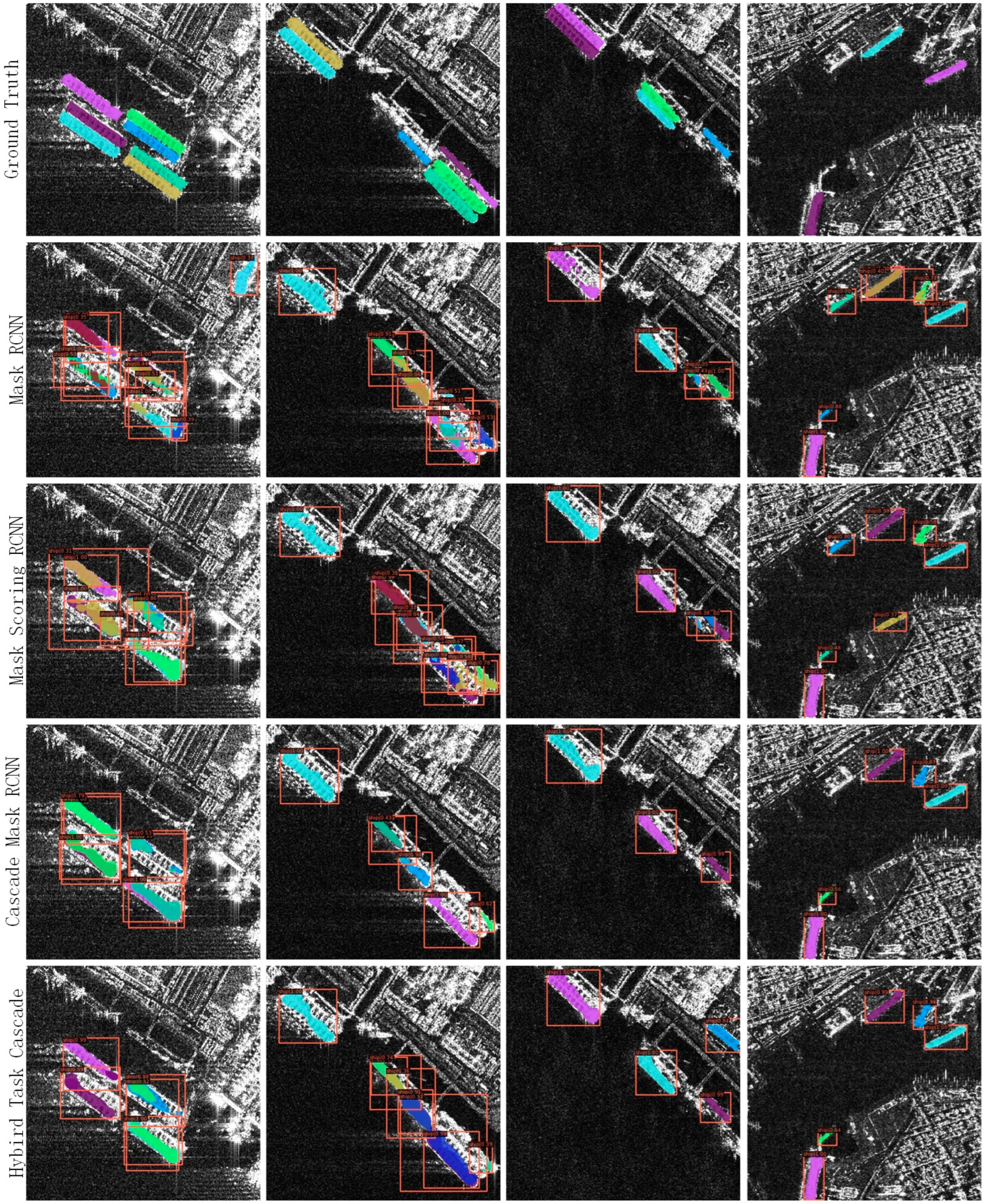
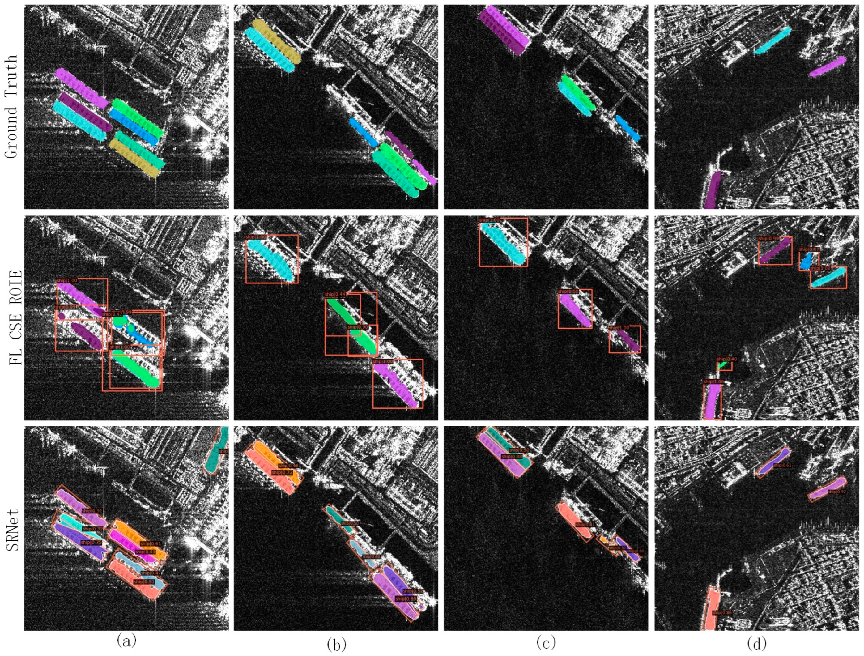
Four visualization illustration images of different comparison networks for instance segmentation on the SSDD dataset. (a) The scene of parallel ships berthing at a dock. (b,c) The scenes of multiple parallel ships berthing on both sides of a dock. (d) The scene of multiple ships sailing in the water region.
Figure 15.
Four visualization illustration images of different comparison networks for instance segmentation on the Instance-RSDD dataset. (a–d) The scenes of the ships berthing in the docks.
Figure 15.
Four visualization illustration images of different comparison networks for instance segmentation on the Instance-RSDD dataset. (a–d) The scenes of the ships berthing in the docks.
Figure 16.
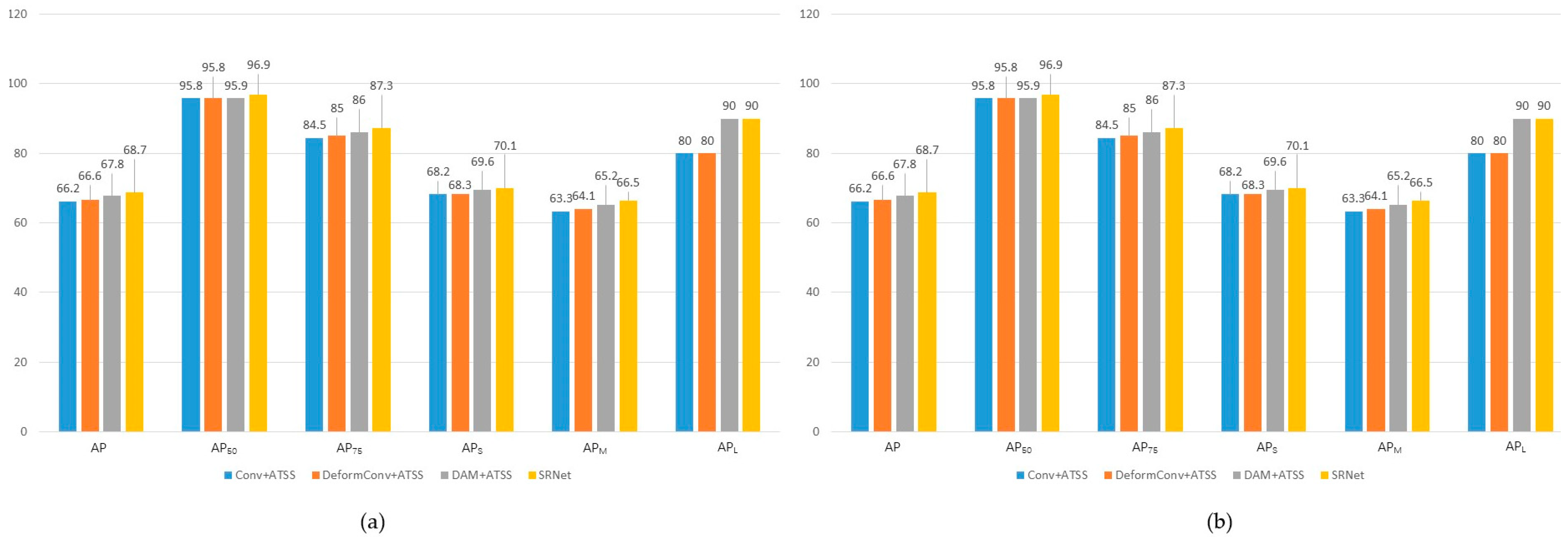
The histograms of ablation experimental results on the SSDD dataset (a) and the Instance-RSDD dataset (b).
Figure 16.
The histograms of ablation experimental results on the SSDD dataset (a) and the Instance-RSDD dataset (b).
Figure 17.
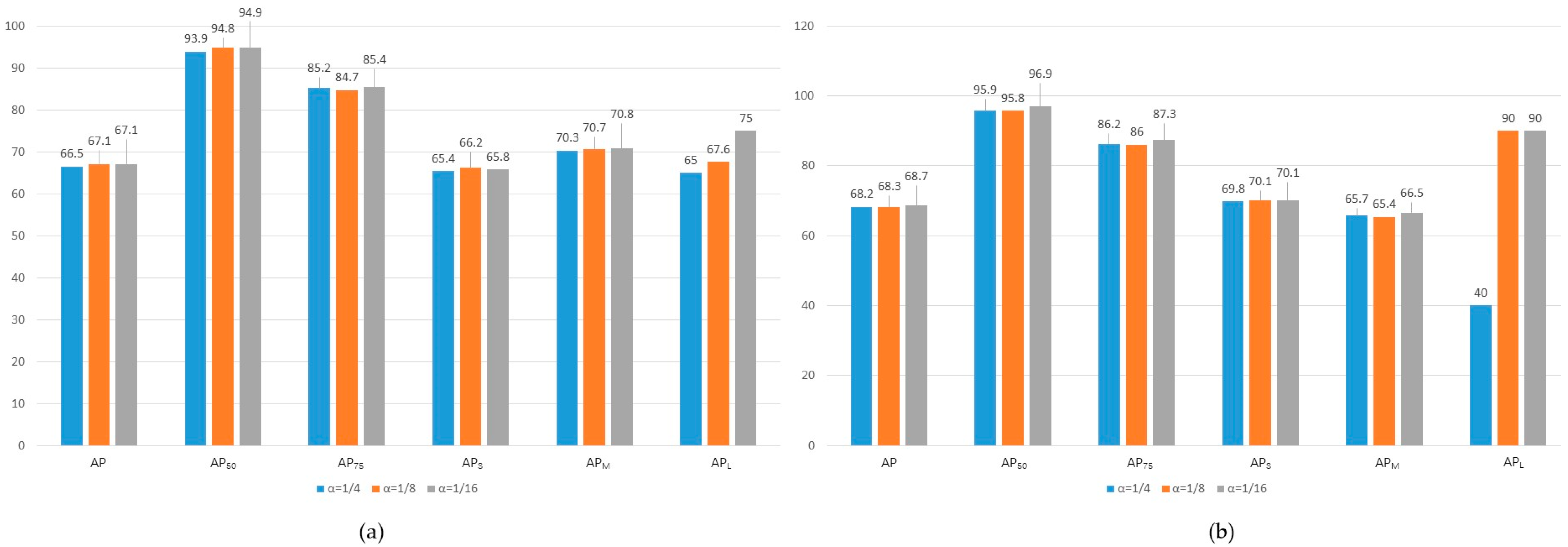
Histograms of the ablation experimental results of factor α on the SSDD (a) and the Instance-RSDD dataset (b).
Figure 17.
Histograms of the ablation experimental results of factor α on the SSDD (a) and the Instance-RSDD dataset (b).
Table 1.
Rotated object detection performance of different networks on the SSDD dataset.
Table 1.
Rotated object detection performance of different networks on the SSDD dataset.
| Networks | Recall | mAP |
|---|
| Rotated Faster RCNN | 92.7 | 89.6 |
| Rotated RetinaNet | 93.0 | 88.6 |
| Rotated Reppoint | 91.0 | 87.5 |
| ROI Trans | 92.9 | 90.1 |
| R3Det | 93.4 | 90.0 |
| ReDet | 94.5 | 90.3 |
| Oriented RCNN | 94.5 | 90.2 |
| S2ANet | 93.8 | 90.0 |
| SRNet | 95.3 | 90.4 |
Table 2.
Rotated object detection performance of different networks on the RSDD dataset.
Table 2.
Rotated object detection performance of different networks on the RSDD dataset.
| Networks | Recall | mAP |
|---|
| Rotated Faster RCNN | 88.2 | 79.2 |
| Rotated RetinaNet | 88.3 | 78.8 |
| Rotated Reppoint | 88.5 | 78.5 |
| ROI Trans | 90.4 | 88.1 |
| R3Det | 89.4 | 80.8 |
| ReDet | 92.5 | 89.3 |
| Oriented RCNN | 90.8 | 88.0 |
| S2ANet | 91.8 | 89.0 |
| SRNet | 92.3 | 89.4 |
Table 3.
Instance-segmentation performance of different networks on the SSDD dataset.
Table 3.
Instance-segmentation performance of different networks on the SSDD dataset.
| Networks | AP | AP50 | AP75 | APS | APM | APL |
|---|
| Mask RCNN | 63.5 | 92.6 | 80.0 | 61.8 | 68.7 | 63.4 |
| Mask Scoring RCNN | 62.6 | 90.7 | 78.8 | 60.8 | 67.8 | 60.1 |
| Cascade Mask RCNN | 64.8 | 93.8 | 79.9 | 63.2 | 69.2 | 53.5 |
| Hybrid Task Cascade | 62.4 | 92.8 | 78.4 | 60.9 | 67.3 | 56.8 |
| FL CSE ROIE | 63.5 | 92.9 | 80.1 | 62.5 | 66.8 | 45.2 |
| SRNet | 67.1 | 94.9 | 85.4 | 65.8 | 70.8 | 75.0 |
Table 4.
Instance-segmentation performance of different networks on the Instance-RSDD dataset.
Table 4.
Instance-segmentation performance of different networks on the Instance-RSDD dataset.
| Networks | AP | AP50 | AP75 | APS | APM | APL |
|---|
| Mask RCNN | 67.5 | 95.8 | 85.7 | 69.8 | 63.1 | 80.0 |
| Mask Scoring RCNN | 68.0 | 95.6 | 86.1 | 70.6 | 63.9 | 70.0 |
| Cascade Mask RCNN | 67.9 | 95.8 | 85.9 | 69.8 | 64.4 | 70.0 |
| Hybrid Task Cascade | 67.9 | 95.8 | 86.4 | 69.6 | 64.8 | 80.0 |
| FL CSE ROIE | 67.7 | 95.9 | 85.7 | 69.2 | 64.8 | 80.0 |
| SRNet | 68.7 | 96.9 | 87.3 | 70.1 | 66.5 | 90.0 |
Table 5.
Ablation experiment results of our network framework on the SSDD dataset.
Table 5.
Ablation experiment results of our network framework on the SSDD dataset.
| Networks | AP | AP50 | AP75 | APS | APM | APL |
|---|
| Conv+ATSS | 64.8 | 94.9 | 81.5 | 64.5 | 66.3 | 72.5 |
| DeformConv+ATSS | 65.6 | 94.9 | 81.9 | 64.4 | 69.9 | 67.6 |
| DAM+ATSS | 66.9 | 94.9 | 84.2 | 65.7 | 71.1 | 65.0 |
| SRNet | 67.1 | 94.9 | 85.4 | 65.8 | 70.8 | 75.0 |
Table 6.
Ablation experiment results of our network framework on the Instance-RSDD dataset.
Table 6.
Ablation experiment results of our network framework on the Instance-RSDD dataset.
| Networks | AP | AP50 | AP75 | APS | APM | APL |
|---|
| Conv+ATSS | 66.2 | 95.8 | 84.5 | 68.2 | 63.3 | 80.0 |
| DeformConv+ATSS | 66.6 | 95.8 | 85.0 | 68.3 | 64.1 | 80.0 |
| DAM+ATSS | 67.8 | 95.9 | 86.0 | 69.6 | 65.2 | 90.0 |
| SRNet | 68.7 | 96.9 | 87.3 | 70.1 | 66.5 | 90.0 |
Table 7.
Ablation experiment results of factor α on the SSDD dataset.
Table 7.
Ablation experiment results of factor α on the SSDD dataset.
| α | AP | AP50 | AP75 | APS | APM | APL |
|---|
| 1/4 | 66.5 | 93.9 | 85.2 | 65.4 | 70.3 | 65.0 |
| 1/8 | 67.1 | 94.8 | 84.7 | 66.2 | 70.7 | 67.6 |
| 1/16 | 67.1 | 94.9 | 85.4 | 65.8 | 70.8 | 75.0 |
Table 8.
Ablation experiment results of factor α on the Instance-RSDD dataset.
Table 8.
Ablation experiment results of factor α on the Instance-RSDD dataset.
| α | AP | AP50 | AP75 | APS | APM | APL |
|---|
| 1/4 | 68.2 | 95.9 | 86.2 | 69.8 | 65.7 | 40.0 |
| 1/8 | 68.3 | 95.8 | 86.0 | 70.1 | 65.4 | 90.0 |
| 1/16 | 68.7 | 96.9 | 87.3 | 70.1 | 66.5 | 90.0 |
