Analysis and Verification of Building Changes Based on Point Clouds from Different Sources and Time Periods

Abstract

Detecting changes in buildings over time is an important issue in monitoring urban areas, landscape changes, assessing natural disaster risks or updating geospatial databases. Three-dimensional (3D) information derived from dense image matching or laser data can effectively extract changes in buildings. This research proposes an automated method for detecting building changes in urban areas using archival aerial images and LiDAR data. The archival images, dating from 1970 to 1993, were subjected to a dense matching procedure to obtain point clouds. The LiDAR data came from 2006 and 2012. The proposed algorithm is based on height difference-generated nDSM. In addition, morphological filters and criteria considering area size and shape parameters were included. The study was divided into two sections: one concerned the detection of buildings from LiDAR data, an issue that is now widely known and used; the other concerned an attempt at automatic detection from archived aerial images. The automation of detection from archival data proved to be complex, so issues related to the generation of a dense point cloud from this type of data were discussed in detail. The study revealed problems of archival images related to the poor identification of ground control points (GCP), insufficient overlap between images or poor radiometric quality of the scanned material. The research showed that over the 50 years, the built-up area increased as many as three times in the analysed area. The developed method of detecting buildings calculated at a level of more than 90% in the case of the LiDAR data and 88% based on the archival data.

1. Introduction and Literature Review

The detection of urban land use changes is very important for monitoring the status of land use development. Such analyses should be performed at short time intervals to achieve regularity of observations. Land use change analysis is a relatively simple technique for comparing two or more maps from different periods. One of the techniques for obtaining maps for comparison is land use classification. The determination of land use can be derived from image data, i.e., orthophotos, satellite imagery, or pseudorasters, obtained from point clouds. This approach involves deciding which pixels from the image should be included in a particular land use class. In the present study, the concentration is on building detection, since it is urban development that is growing at a relatively fast pace and often becomes the dominant feature in the immediate landscape. As a consequence, green areas are disappearing and the chaotic sprawl of buildings is occurring, causing a number of potential hazards in the form of space degradation [1]. The uncontrolled development of land in Poland was observed after 1989 [2]. In response to the emerging development, documents began to be created to prevent inappropriate land development. Urban planning has become the primary land use policy document to ensure order in individual local government units [3]. The monitoring of built-up areas has become an important research subject and was a motivation for this work. In the present study, a detection of the changes in development that have occurred over several decades in the context of spatial planning was carried out. It was assumed that modern measurement tools would make it possible to quickly and accurately show how cities grew and whether they caused significant disruption to the landscape.

The theme of urban change detection is discussed in many articles. The authors mainly concentrate on the analysis of image data—aerial and satellite images. Urban change detection for the period of 1978–2017 at Kolkata is presented in [4]. The supervised Maximum Likelihood Classification technique is used to classify the multi-temporal satellite data in five classes, which are urban built-up, open land, vegetation, agricultural land and water body. In [5], the proposed method realises the spatial–temporal modelling and correlation of multitemporal remote sensing images through a coupled dictionary learning module and ensures the transferability of reconstruction coefficients between multisource image blocks. In [6], a novel supervised change detection method is proposed based on a deep Siamese convolutional network for optical aerial images. The novelty of the method is that the Siamese network is learned to extract features directly from the image pairs. An interesting solution is to use the Conditional Adversarial Network solution for change detection [7]. The original network architecture based on pix2pix is proposed and evaluated for difference map creation. The principal goal of the research in [8] is to introduce two novel deep convolutional models based on the UNet family for multi-object segmentation, such as roads and buildings from aerial imagery. The presented models are called multi-level context gating UNet (MCG-UNet) and the bi-directional ConvLSTM UNet model (BCL-UNet). The study in [9] proposes a single patch-based convolutional neural network (CNN) architecture for the extraction of roads and buildings from high-resolution remote sensing data. Moreover, the authors in [10] explore the usage of convolutional neural networks for urban change detection using two architectures: Siamese and Early Fusion. The goal of the research in [11] is to create a strategy that enables the extraction of indicators from large-scale orthoimages of different resolution with practically acceptable accuracy after a short training process. The suggested model training process is based on the transfer learning technique and combines using a model with weights pretrained in ImageNet with learning on coarse and fine-tuning datasets. In [12], a convolutional neural network (CNN)-based change detection method is proposed with a newly designed loss function to achieve transfer learning among different datasets. In [13], a generative adversarial networks (GAN)-based method is proposed for the data augmentation of the collected crack digital images and a modified deep learning network (i.e., VGG) for crack classification.

The above methods use only 2D data. An interesting approach to change detection is to integrate 3D data extracted from dense matching or LiDAR data. Reference [14] proposes the combination of image-based dense DSM reconstruction from historical aerial imagery with object-based image analysis for the detection of individual buildings and the subsequent analysis of settlement change. For the case of densely matched DSMs, the evaluation yields building detection rates of 92% for greyscale and 94% for colour imagery. In [15], height difference and greyscale similarity are calculated as change indicators and the graph cuts method is employed to determine changes considering the contexture information. In the study in [16], LiDAR data were used to identify agricultural land boundaries. Paper [17] proposes a change detection method based on stereo imagery and digital surface models generated with stereo matching methodology and provides a solution by the joint use of height changes and Kullback–Leibler divergence similarity measures between the original images. In addition, [18] proposes a feed-forward convolutional neural network (CNN) to detect building changes using ALS and photogrammetric data. The point cloud from dense matching is also used in [19]. The graph cuts algorithm is adopted to classify the points into foreground and background, followed by the region-growing algorithm to form candidate-changed building objects. In [20], a four-camera vision system was built to obtain the visual information of targets including static objects and a dynamic concrete-filled steel tubular (CFST) specimen. In [21], a novel method is proposed to detect changes directly on LOD2 (level of detail) building models with VHR spaceborne stereo images from a different date, with a particular focus on addressing the special characteristics of the 3D models. Publication [22] proposes a multi-path self-attentive hybrid coding network model (MAHNet) that fuses high-resolution remote sensing images and digital surface models (DSMs) for the 3D change detection of urban buildings. In [23], the authors present a semantic-aided change detection method aimed at monitoring construction progress using UAV-based photogrammetric point clouds. A new approach for change detection in 3D point clouds is proposed in [24]. It combines classification and change detection in one step using machine learning. Paper [25] presents a graphical user interface (GUI) developed to support the creation of a building database from building footprints automatically extracted from LiDAR point cloud data. The research in [26] proposes the use of LiDAR-guided dense matching to explicitly address these problems in detecting accurate building changes. Paper [27] shows that point cloud completion improves the accuracy of change detection; the authors perform point cloud completion using a hierarchical deep variational autoencoder (a type of artificial neural network) modified to include skip connections between the convolution and deconvolution layers. A very interesting and in-depth summary of the development and analysis of data and the state-of-art based on deep learning and 3D point clouds is presented in article [28].

A review of the literature shows significant interest in the problem of change detection in urbanised areas. This is an important issue in times of urban sprawl.

However, most of the presented methods only focus on current data: aerial photos, satellite images and LiDAR elevation data, ignoring historical data completely. A review of the literature revealed only a few publications that analysed archival data. This is a major oversight, as urban development should be considered over a wider time period in order to draw correct conclusions. The present study analyses a period of over 50 years of change in the urbanised area in the centre of Krakow. The dynamics of these changes and the exponential growth of the number of buildings in a relatively small area can be seen. The developed method is simple and effective, clearly documenting the major urbanisation of Krakow.

2. Study Area and Materials

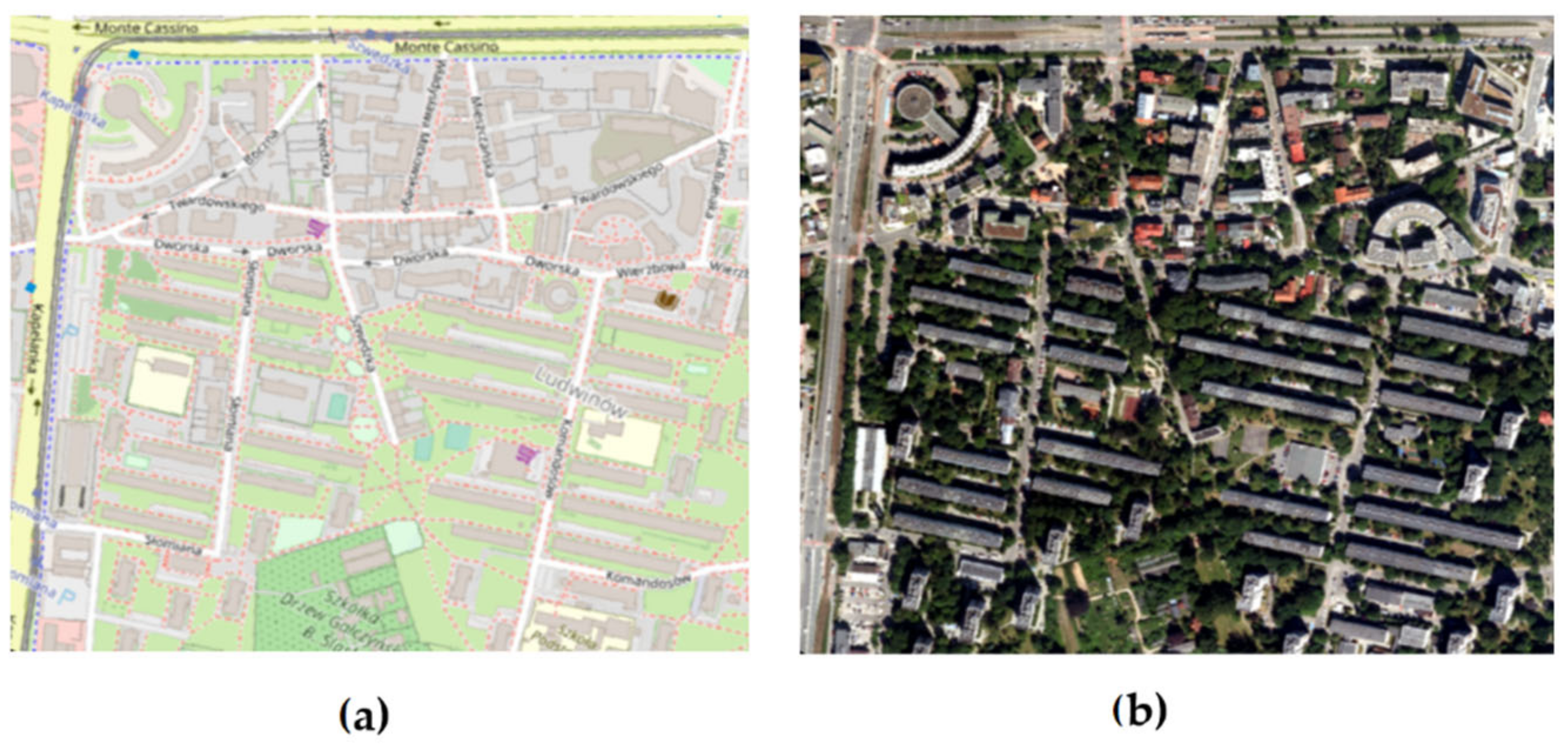
The choice of the test area was not random. The area was completely flooded during the flood in Krakow in 2010. The research answers the question of how much uncontrolled urban sprawl could have caused this disaster. This site is in the centre of Krakow, on the west side of the Wisla River, and covers 9.17 ha. The analysed area includes the Podwawelskie estate, which is located in the southern part, and the area named Monte Cassino—Konopnicka, lying in the northern part (Figure 1). The Podwawelskie estate was established on the territory of the previous villages of Ludwinów and Zakrzówek, which were subsequently incorporated into Krakow in 1910 and 1909 as the IX and X cadastral districts [29]. Currently, the entire study area is part of District VIII Debniki, belonging to the Podgórze cadastral unit. The examined fragment is bounded by Kapelanka Street on the western side, Monte Cassino Street on the northern side and Maria Konopnicka Street on the eastern side. Over the past few decades, the area has been significantly urbanised. At present, there are mainly residential blocks in the shape of cuboids. These buildings have flat roofs, and their heights range from 10 m to 38 m. The area surrounding the blocks is flat and covered with high vegetation.

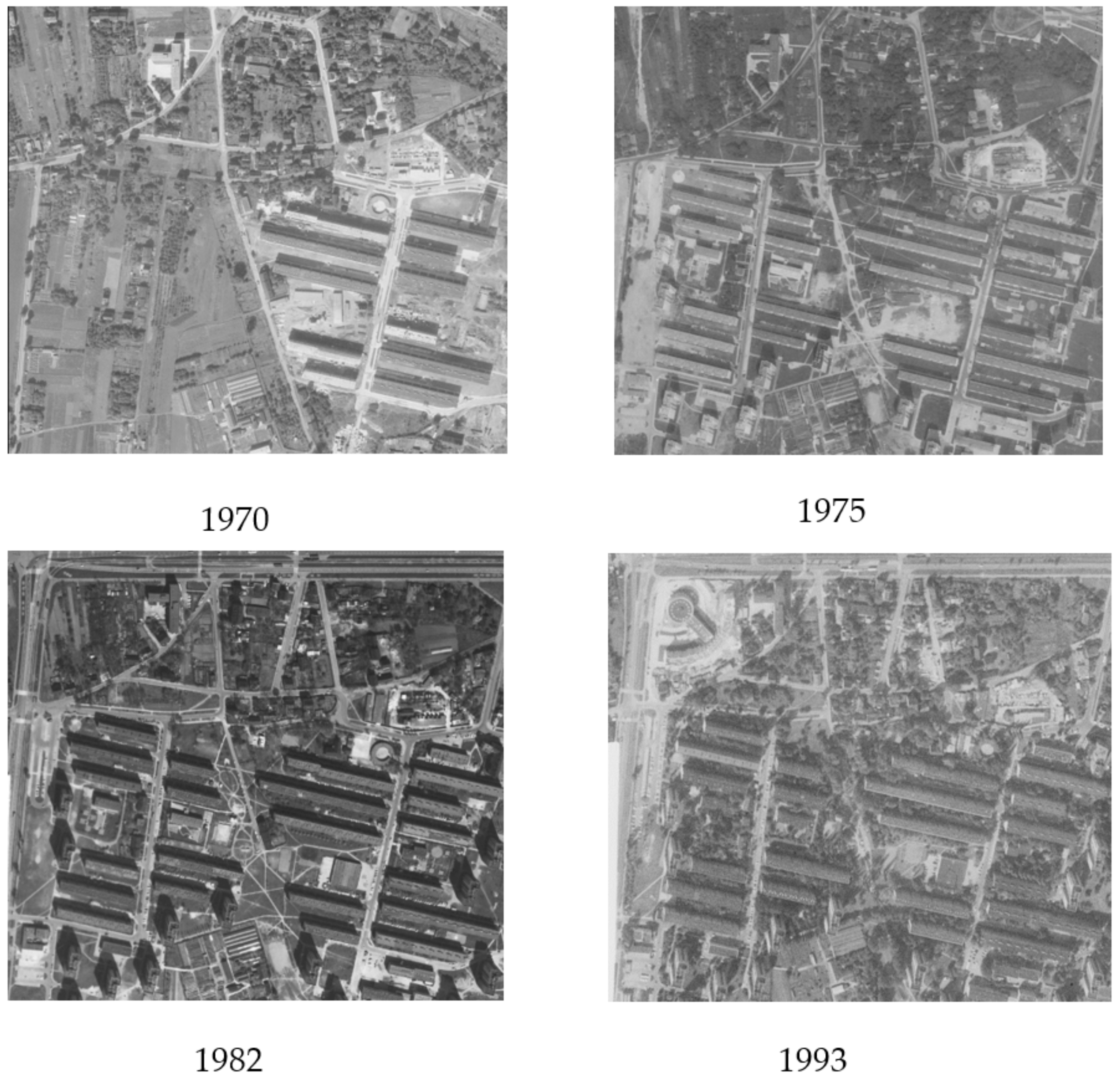
Archival aerial photographs taken between 1970 and 1993 (Figure 2) and data acquired by airborne laser scanning in 2006 and 2012 (Figure 3) were used for the analyses. All archival aerial photographs are greyscale analogue images, characterised by poor radiometric quality and variable scale—from 1:16,000 to 1:30,000 (

Table 1. Specific characteristics of the study data (AP—aerial photograph, LD—LiDAR data, BDOT10k—topographic object data).

Acquisition Date	Type of Data/Scale	Time between Acquisition Dates (Years)	Ground Pixel Resolution (m)	Points per m2
1970	AP black/white (1:18,000)	-	0.25	-
1975	AP black/white (1:17,000)	5	0.23	-
1982	AP black/white (1:16,000)	7	0.21	-
1993	AP black/white (1:30,000)	11	0.40	-
2006	LD X, Y, Z	13	-	4–7
2012	LD X, Y, Z, intensity, echo, RGB	6	-	6–12
2020	BDOT10k	8	-	-

). Additionally, the current BDOT10k (Topographic Objects Database) database was used for verification purposes. This is a vector database containing the spatial location of topographic objects together with their basic descriptive characteristics [30].

The first set of LiDAR data is from a survey carried out in 2006, where the Fli-Map system was used. The point density is variable, ranging from 4 to 14 points per m². This means that the topography and all details of the covering elements are reproduced with high precision. A second set of LiDAR data was acquired in 2012 as part of the Polish ISOK project (IT System of the Country’s Protection Against Extreme Hazards) [31], whose point density was 12 points per m². Both datasets are recorded in the 92 coordinate system and the area analysed includes the following sheets: M-34-64-D-d-1-4-3-2, M-34-64-D-d-1-4-4-2, M-34-64-D-d-1-4-4-1, M-34-64-D-d-3-2-2, M-34-64-D-d-1-4-4, M-34-64-D-d- M-34-64-D-d-3-2-1-2, M-34-64-D-d-3-2-2-1, M-34-64-D-d-1-4-3-4 and M-34-64-D-d-1-4-4-3 (Figure 3, Table 1).

3. Methodology

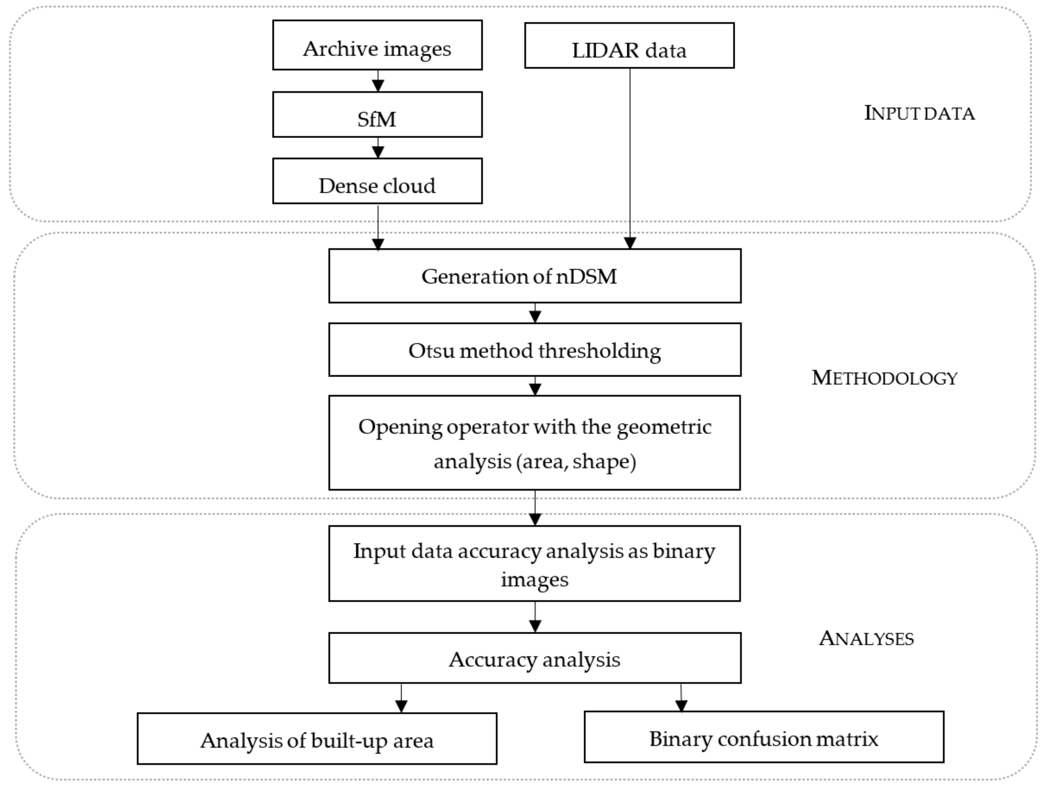
Based on a very large set of source data covering 50 years of development in the centre of Krakow, it was decided that a simple and fast change detection method would be chosen. The proposed algorithm was based on the analysis of a normalised digital surface model (nDSMs). The nDSM is a representation of the terrain surface along with objects extending above that surface, such as buildings and trees. In this case, the nDSM was obtained from point clouds extracted from the dense matching of archival images and directly from laser data. However, before the final nDSM could be generated, proper processing of the input data was required. To obtain the nDSM from the images, aerotriangulation is required and then a dense matching is carried out. On the other hand, the point cloud from LiDAR must be classified correctly. Having correctly generated point clouds, it is possible to generate the nDSM from them. The generation of nDSM is carried out with the use of the morphological operators, surface and shape analysis criteria. All measurements and calculations were conducted in Agisoft Metashape, QGIS, SAGA, GRASS and Orfeo ToolBox software. The proposed method of data analysis and processing is illustrated schematically in Figure 4.

4. Generation of nDSM

4.1. Generation of nDSM Using Archival Data

In the first step, to obtain point clouds from archival images, adjustment and dense matching were performed.

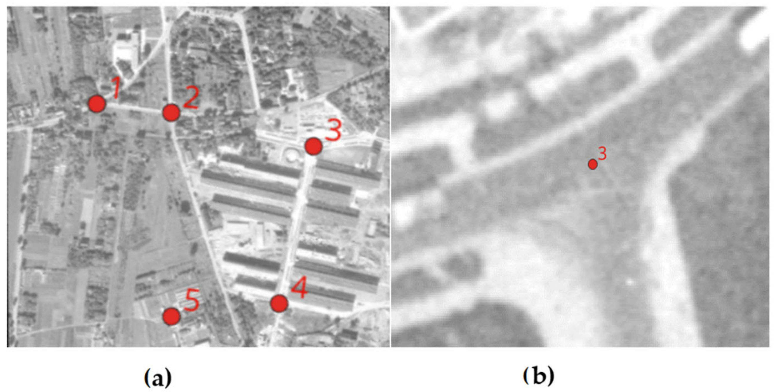
The adjustment was carried out using five GCPs measured from archival images (Figure 5a). This task was quite complicated, since in the 1970s, there were a lot of agricultural areas in the study region, without characteristic ground details. Five GCPs were selected to have redundant observations and to determine the georeferencing accuracy. Attempts were made to place points in the corners and the centre of the area. Unfortunately, due to the impossibility of identifying the same points in all years, it was not completely achievable. Attempts were made to select GCPs at road intersections, but due to the poor radiometric quality of the archival images, this measurement was not always unambiguous (Figure 5b).

Due to problems with the precise identification of GCP (especially for 1993), a mean RMSE of 10 pixels was set as acceptable. The detailed adjustment results are included in

Table 2. SFM block bundle adjustment results.

Year	Number of GCPs	Tie Points	Reprojection Error (pix)	Mean RMSE (pix)
1970	5	495	0.96	2.69
1975	5	1688	0.20	1.02
1982	5	2247	2.47	10.03
1993	5	1513	1.67	8.71

.

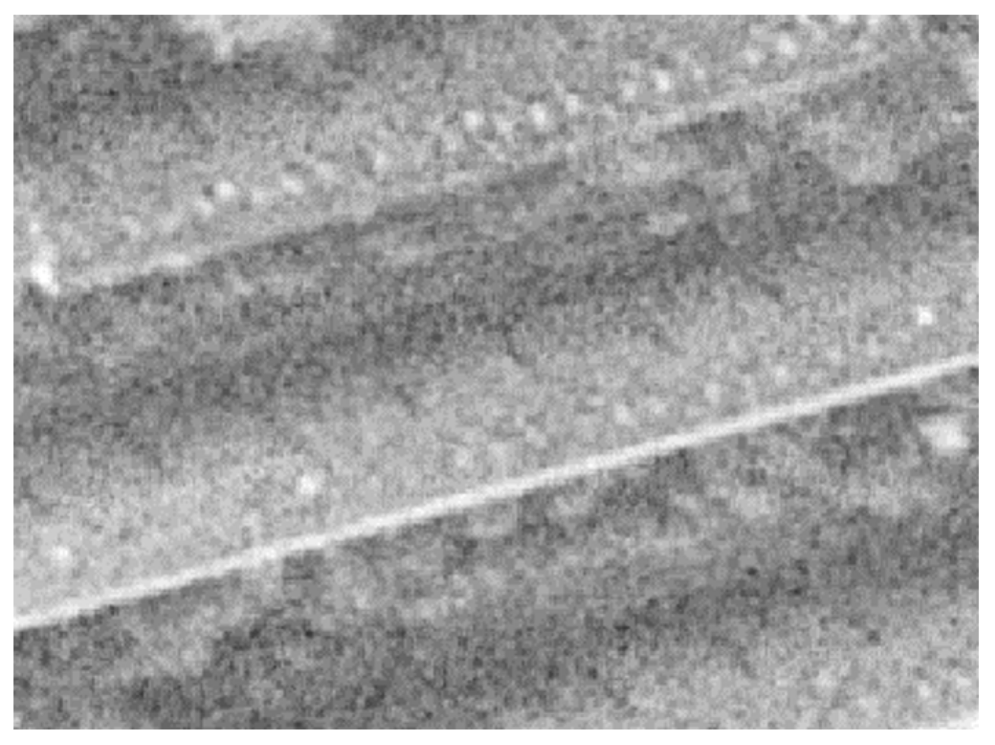
The dense point clouds differed significantly in quality. The best results were obtained for 1975, where the correct radiometry and large scale of the images made it possible to generate a cloud of high quality and density. Significant problems were encountered for the data from 1993. Unfortunately, the images from this period had very poor radiometric quality and high noise and carrying out the procedure of dense matching did not bring satisfactory results. An example of two buildings, surrounded by vegetation, in a 1993 image is shown in Figure 6. As can be seen, the high graininess of the image and the similar brightness of the pixels actually prevent the correct identification of the objects.

A significant challenge in generating dense clouds for all of the dates considered were the wooded areas, which had very similar brightness in the halftone images. The dense clouds acquired for these fragments were characterised by ragged information and erroneous height values (Figure 7).

The problem of the poor radiometric quality of historical images is an important research issue. However, the purpose of this study was to detect changes in buildings over 50 years. Future research will be devoted to improving the radiometry of scanned analogue images.

The quality of the point clouds was also affected by the overlap between successive images. Unfortunately, a complete set of historical data was not always available, and a small percentage of overlap affected the density of the acquired cloud.

Based on the dense point cloud, a 0.5 m digital surface model (DSM) nearest neighbour method was interpolated. In order to better identify the development in the analysed area, it was decided to determine the normalised digital surface model (nDSM). To realise this, an actual digital surface model (DTM) derived from the ISOK project with a field resolution of 0.5 m was used [31].

4.2. Generation of nDSM Using Lidar Data

To extract information about buildings from LiDAR data, it is necessary to classify the point cloud. Classification is the assignment of appropriate attributes to points, considering their relative heights. Height classification was carried out on data from 2006. First, point filtering was performed, that is, searching for points representing terrain using the active model triangulation method [32]. Next, points representing vegetation were grouped, relative to height, into low, medium and high vegetation. Height was defined as the distance of the point from the ground. The final step was to find points reflected from buildings. Data from 2012 were obtained from the National Geoportal [31], which had already been clustered. Having the data classified, height models—DTM and DSM—were built using the interpolation of scattered points to a regular 0.5 m grid, where the interpolation neighbour method was used. Points belonging to the “Ground” layer were used to build the first model (DTM), while the second model (DSM) was unusual because was only generated from points belonging to the “Buildings” layer. The normalised digital surface model is a differential model that represents the relative heights of objects projecting above the ground surface, so it was calculated as the difference between the DSM and DTM models. As a result, two rasters with relative values of the analysed area were obtained.

5. Building Detection

5.1. Otsu Method Thresholding

The Otsu algorithm is used for thresholding method segmentation [33]. The purpose of it is to select the optimal threshold for image binarisation. A criterion function is used for optimisation, which is the intra-class variance (it is minimised), or the inter-class variance (it is maximised). Assuming that the image pixels are divided into two classes C₀ and C₁ by the boundary value n, then C₀ will contain pixels with brightness [1, ..., n], and C₁ will contain pixels with brightness [n + 1, ..., L], where L is the maximum value of a pixel and p_i is equal to the ratio of the number of pixels with a given value i to the number of all pixels in the image. The class probability (normalised histogram value) for C₀ and C₁, respectively, will be:

$${\omega }_0={\displaystyle \sum }_{i=1}^n{p}_i$$

(1)

$${\omega }_1={\displaystyle \sum }_{i=n+1}^L{p}_i$$

(2)

The inter-class variance is taken as the criterion function, aiming to maximise it. It is expressed by the formula:

$${\sigma }_B^2={\omega }_0{\left({\mu }_0-{\mu }_T\right)}^2+{\omega }_1{\left({\mu }_1-{\mu }_T\right)}^2$$

(3)

where:

μ₀—C₀ mean;

μ₁—C₁ mean;

μ_T—the total average level.

The value of n for which the value of the inter-class variance is the largest is the searched optimal threshold for the image.

5.2. Opening Operator and Geometry Analysis

The next step in the algorithm is to perform a morphological opening operation on the image obtained after thresholding [34]. The resulting image A is given an erosion and then dilation using structural element B:

$$A\circ B=\left(A⊝B\right)⨁B$$

(4)

Opening removes small objects and fine details, such as peninsulas and protrusions, and disconnects some objects with constrictions. However, it does not affect the basic shape of the object. In the case of point clouds from archival images, this was a very helpful step due to the high noise of the information and the creation of many false artifacts. The operator was enhanced with two additional criteria: surface analysis and the shape of the detected objects. The threshold for the minimum building area was set at 25 m². The second criterion concerned the geometry of the building, and the rectangularity parameter was determined based on Formula (5):

$$R=\frac{A}{a+b}$$

(5)

where:

A—the area of the object;

a, b—sides of the smallest rectangle in which the object can be contained.

The study assumed a threshold for R > 0.6.

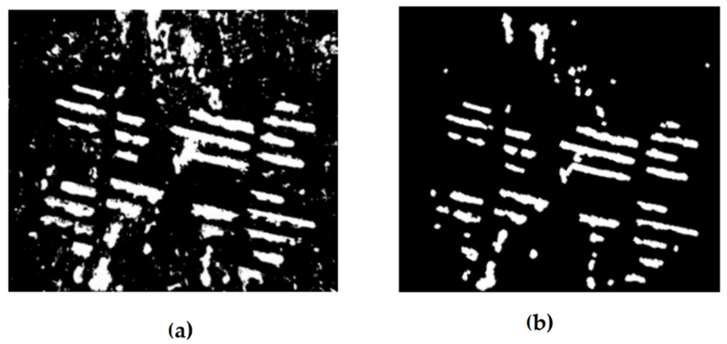
Performing additional operations was necessary, especially for the archive images, which were characterised by a lot of noise in the clouds. An example of the above-mentioned operators on building detection in 1975 is shown in Figure 8.

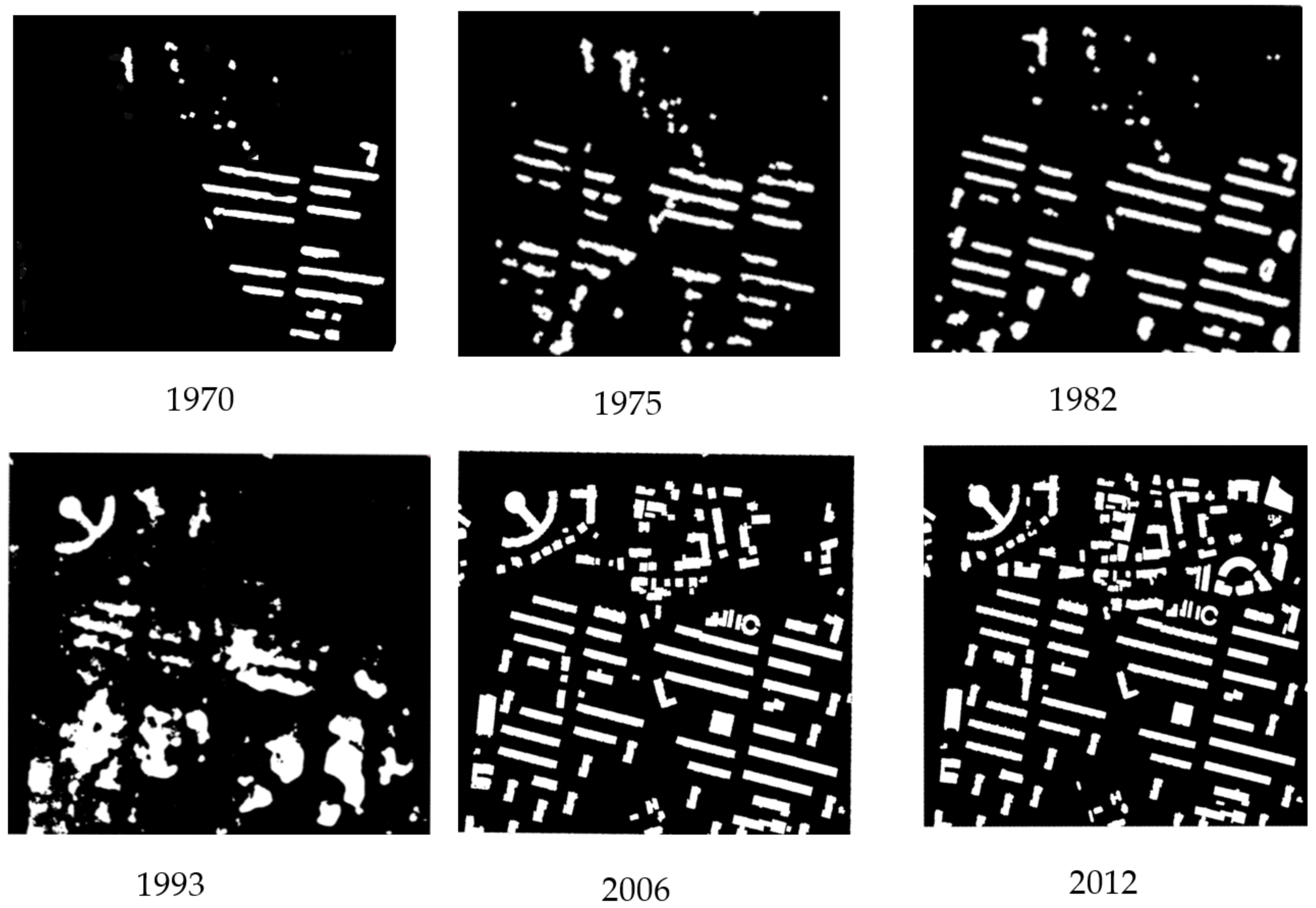
As a result of the developed algorithm, binary images were obtained, which included the two classes “Building” and “Non-building”. For each time period, a separate binary image with detected buildings was created (Figure 9).

Figure 9 shows very large errors for the year 1993. This was caused by the very poor radiometric resolution of the images and the small scale—1:30,000, as discussed in Section 4.1. It was therefore decided to omit this year from further study.

6. Results and Discussion

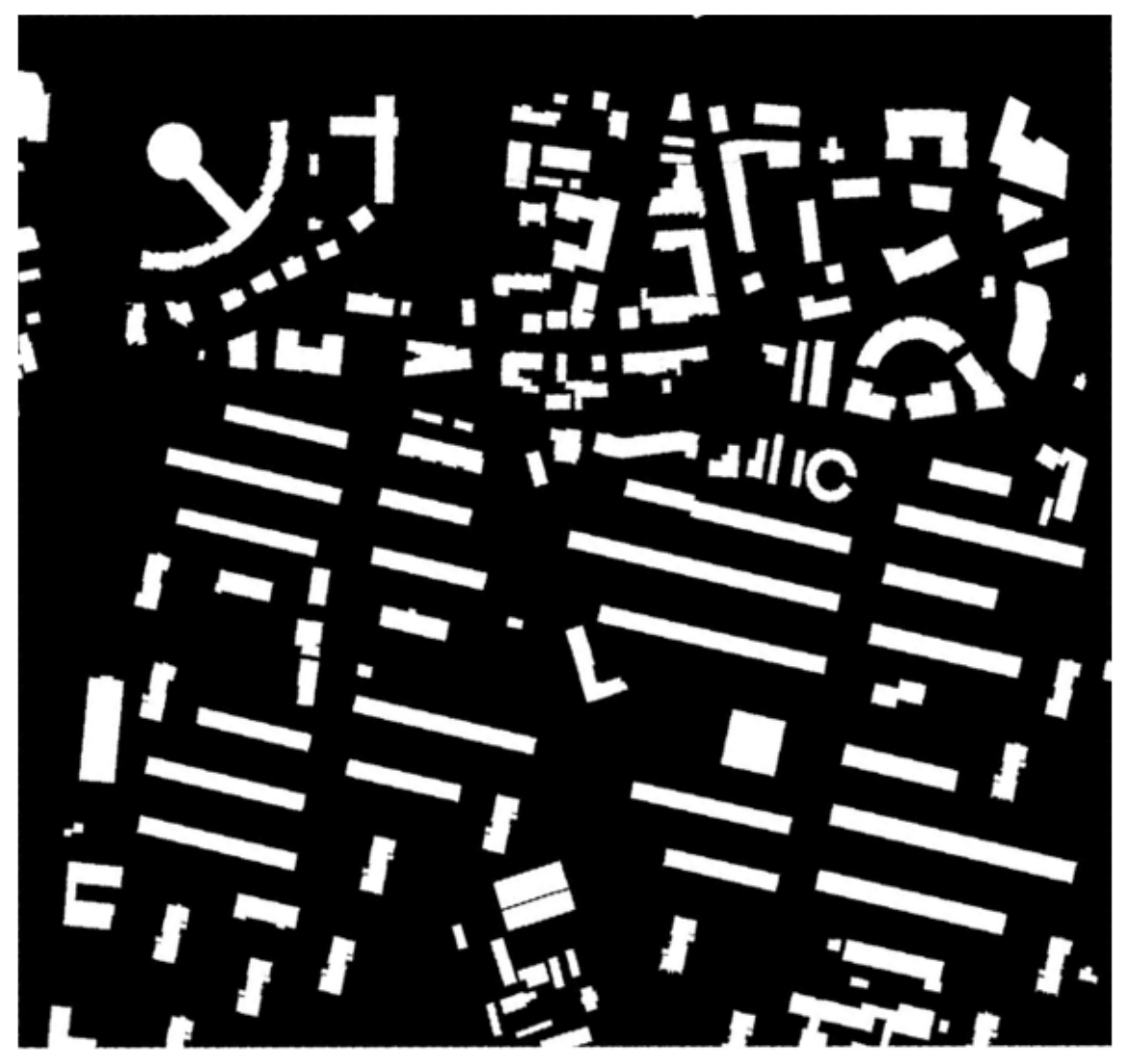
All years were compared with buildings extracted from the topographic objects database from the OT_BUBD_A layer of 2020. The file containing the vector description of the buildings was rasterised, producing a raster with two layers: “Building” and “Non-building”. The result is presented in Figure 10.

The first analysis of the collected data is the quantitative analysis. The pixel area of the “Building” class was calculated, i.e., that which represents the area in which buildings can be found. Then the percentage of buildings in relation to the total analysed area was calculated (

Table 3. Area of “Building” and “Non-building” classes and percentage of built-up area in relation to the whole study area.

		1970	1975	1982	2006	2012	2020
Building Area	(m2)	28,317	38,148	53,655	73,210	84,295	85,332
Non-Building Area	(m2)	475,052	465,221	449,714	430,159	419,074	418,037
Percentage of built-up area	(%)	5.6	7.6	10.6	14.5	16.7	17.0

). The total area of the entire analysed region is 503,369 m². The area of the buildings, as well as of the whole area, was rounded to 1 m².

Analysing the above table, it can be seen that the development area has increased more than three times over several decades. From the above table it can be seen that the area of development every few years increases by 3–4%, on average.

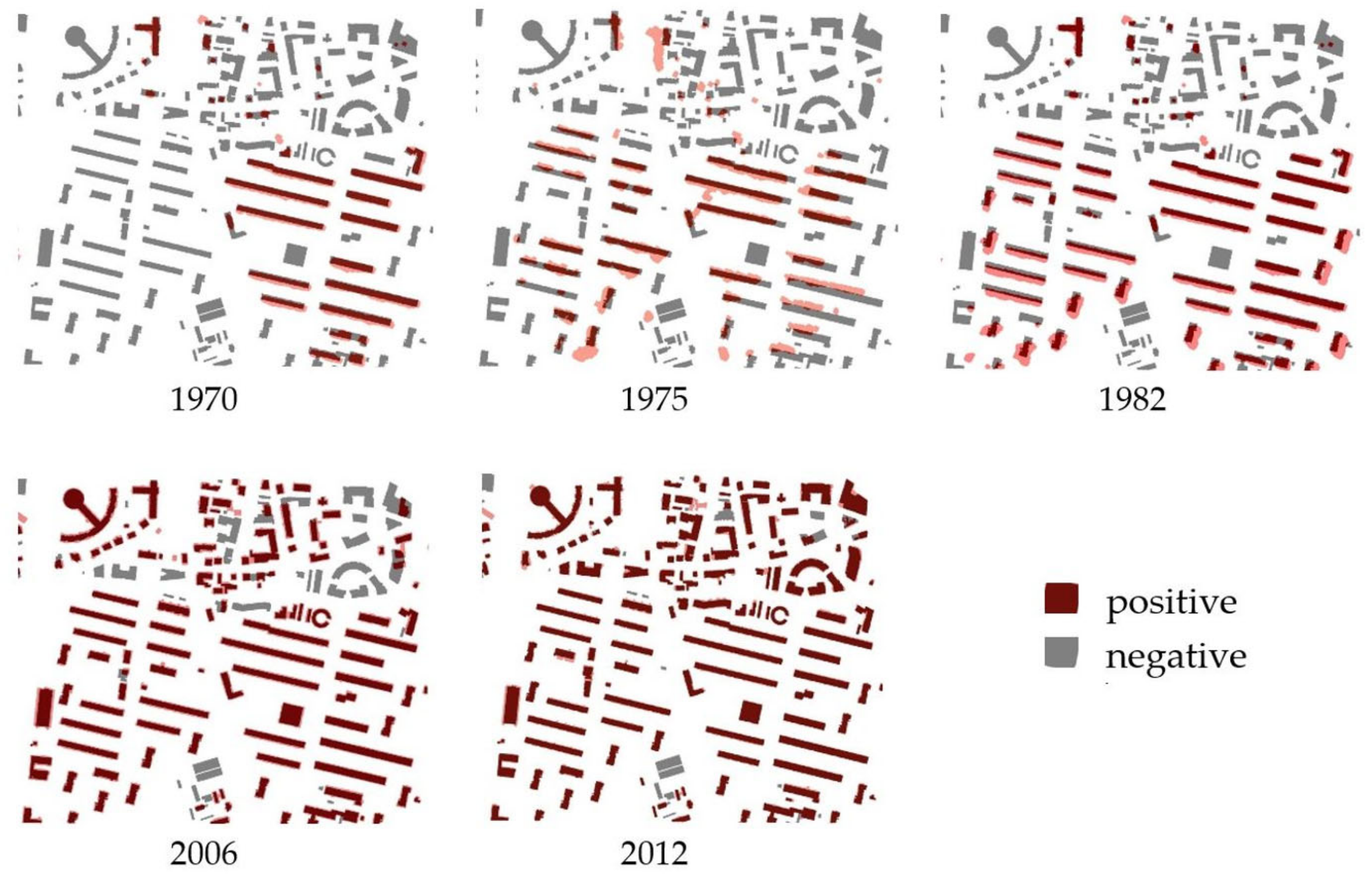
Figure 11 presents the results that show the detected buildings for each year. All data were compared with a reference, i.e., 2020 buildings from BDOT. In the images, red indicates is a positive site, i.e., where the building is present, and grey sites are negative sites, i.e., there was no building at a given time, but now there is.

In order to precisely verify the detection results, confusion matrices were calculated. When building the confusion matrix, data from 2020 were used as a reference. Five confusion matrices were calculated, one for each period. The binary confusion matrix is a 2 × 2 matrix, which contains information, i.e., the number of pixels correctly classified as a “Building” (TP—true positives), correctly not classified as a “Building” (TN—true negatives), falsely classified as a “Building” (FP—false positives) and falsely not classified as a “Building” (FN—false negatives). One binary confusion matrix is assigned to one period. An example matrix is given for the time period 1970 (

Table 4. Binary confusion matrix for 1970. Pixel-by-pixel comparison results.

Confusion Matrix	Reference Map
Our Results	Building	Non-Building	Total
Building	1,639,728 (TP)	32,589 (FP)	1,672,317
Non-Building	258,028 (FN)	80,900 (TN)	338,928
Total	1,897,756	113,489	2,011,245

). In our case, we have five binary confusion matrices (one for each time period), where each matrix has been flattened and written in one row (

Table 5. Binary confusion matrix for all analysed years with parameters defining the quality of building detection.

Years	TP	TN	FP	FN	TPR	PPV	ACC	ERR	F1
1970	1,639,728	80,900	32,589	258,028	0.8640	0.9805	0.8555	0.1445	0.9186
1975	1,598,977	79,155	73,240	259,873	0.8602	0.9562	0.8344	0.1656	0.9057
1982	1,585,320	127,480	86,949	211,496	0.8823	0.9480	0.8516	0.1484	0.9140
2006	1,558,810	259,067	113,621	79,747	0.9513	0.9321	0.9039	0.0961	0.9416
2012	1,609,333	314,500	63,097	24,315	0.9851	0.9623	0.9565	0.0435	0.9736

). The graphical presentation of the results is shown in Figure 12.

In addition, parameters defining the quality of detection were calculated for each confusion matrix, which are listed in the right part of Table 5. The indicators that were calculated are presented in

Table 6. Selected accuracy indicators calculated for each time period [35,36].

Description	Acronym	Formula
Sensitivity (True positive rate)	TPR	$\frac{TP}{TP+FN}$
Precision (Positive predictive value)	PPV	$\frac{TP}{TP+FP}$
Accuracy	ACC	$\frac{TP+TN}{TP+TN+FP+FN}$
Error	ERR	$\frac{FP+FN}{TP+TN+FP+FN}$
F1 score	F1	$\frac{2\times TPR\times PPV}{TPR+PPV}$

, below.

Upon analysing the above results, the following conclusions can be reached. The calculated values of the true positive rate parameter (sensitivity) are in the range from 86% to 98%. This parameter determines what percentage the true positive class, in our case the detection of the “Buildings” layer, was covered by the positive prediction. It can be seen that in the case of building detection, the LiDAR-acquired data are at a high level. Detection using archival images was found to be weaker, but here, the error is certainly influenced by the complex preparation of the input data. However, despite these disadvantages, it is an excellent source of data from which it is possible to verify the coverage of an area quickly and automatically with buildings as it was several decades ago.

The overall accuracy (ACC) of the presented building detection algorithm using data from different sources is, on average, 88%, which shows the percentage of correctly classified pixels. However, again, the accuracy of the detected buildings using LiDAR data is much higher. The detection of buildings from archival images is at a level well above 80%, which is a satisfactory result.

For each dataset, the positive predictive value (PPV) is above 93%. This value determines what percentage of the detected buildings for each dataset overlap with the buildings in the reference image. Thus, a high PPV value indicates high precision on building detection for each time set.

The error rate (ERR) is small for the LiDAR data at less than 10%. On the other hand, for archived data, it is not much higher, but this was to be expected since the input dataset was much less accurate.

In addition, confirmation of the correct operation of the algorithm is the F1 score parameter, which is above 0.9 for each case.

7. Conclusions

Urban development is growing at a very fast pace. As a consequence, green areas and permeable areas are disappearing, and there is a chaotic expansion of development, causing a number of potential dangers in the form of space degradation. The monitoring of these areas has become an important issue and motivated the present research work.

This paper proposes a method for detecting changes in development over 50 years. Archival aerial imagery and LiDAR data were used for this purpose—the dataset covered six time periods: 1970, 1975, 1982, 1993, 2006 and 2012.

The choice of the test area was not random. The area was completely flooded during the 2010 Krakow floods. The study revealed three times the number of buildings in the analysed area, which may be one of the reasons for the flooding of the area. Such data are an excellent source of information for local governments involved in urban planning.

A review of the literature revealed that most publications focus on change detection using 2D aerial and satellite images. The use of 3D information in this process significantly enhances the ability to identify and correctly interpret changes in the analysed area.

A key step was the extraction of 3D information from archival images. Both alignment and dense matching presented a major challenge. When aligning historical photographs, it is important to remember to correctly identify the GCPs, which must be elements that have not changed over 50 years. A considerable problem is also often the poor radiometric quality of such images or missing data, which results in the density and quality of the generated point cloud. The approach presented here makes it possible to reconstruct the heights of buildings in particular years, thereby improving the interpretive possibilities of analogue images. The resulting point clouds reproduce the three-dimensional reality of the city more than half a century ago.

Detecting buildings using LiDAR data is a well-known, frequently used task, and the results obtained are at a high level. This was also confirmed by the present study, since for the time periods for which there are point clouds from airborne laser scanning, the detection of buildings was above 90%.

The accuracy metric calculated in this study is reliable and works well for the case of classifying one class—in our study it was buildings. For the analysed area, the calculated average ACC value was 88%, which is a satisfactory result since the input data were of different quality. It is also worth noting that automatic detection was taken in an area with differentiated roofs, including flat, two- or four-pitched and round roofs, and areas that were covered with tall trees at different times. Detecting such diverse objects in a complex terrain is much more difficult.

The proposed algorithm is not perfect and requires improvements, e.g., improving the radiometry of archival images for better detection of buildings.

The present study shows that, given a diverse set of input data, it is possible to make an automatic analysis of urban land use over several decades. This method is ideal for urban planning and assessment of infrastructure development and can also be an informational element for local governments in urban planning.