
Global and Local Graph-Based Difference Image Enhancement for Change Detection
Abstract
1. Introduction
1.1. Background
1.2. Related Work
1.2.1. DI of Homogeneous Optical Images
1.2.2. DIs of Homogeneous SAR Images
1.2.3. DI of Heterogeneous CD
- Different CD problems face different challenges. (1) For the CD of homogeneous optical images, its difficulty lies in that, when the image resolution is very high, the great intraclass variation and low interclass variance as well as the influence of illuminations and seasons can lead to a lot of salt-and-pepper noise [7]. (2) For the CD of homogeneous SAR images, its difficulty lies in the inherent speckle noise and high intensity variation that can lead to difficult trade-offs between noise removal and geometrical detail preservation in the DI. (3) For the heterogeneous CD, the key lies in how to construct relationships between heterogeneous images so that incomparable images can be compared; it also faces the challenges of both the homogeneous CD of optical images and SAR images.
1.3. Motivations
- Most of these methods are for the conventional denoising and smoothing of DI and they only exploit the information of the DI itself, such as the change information (pixel value) and spatial context information, while ignoring the specificity of the change detection task and neglecting the information in the original multi-temporal images, which limits their performance.
- Most of the methods only serve as “icing on the cake” for smoothing the DI, but cannot further correct the DI. For example, when there is an overall error in the local area in the DI, i.e., when the pixel values of the entire local area that really changed are all 0 in the DI or when the pixel values of the entire local area that really unchanged are all 1, it is difficult to correct this error based on the spatial smoothing or filtering operations.
1.4. Contributions
- First, we have designed a DI-enhancement algorithm specifically for the change detection task, which is a plug-and-play approach for DI post-processing. This is a rarely found work specifically designed for smoothing and correcting DIs in CD problems.
- Second, the proposed DI-enhancement algorithm, named GLGDE for short, not only can smooth the DI but also correct it by using the constructed global feature graph and local spatial graph, which can fully fuse and utilize the change and contextual information in the DI and correlation information in the multi-temporal images.
- Third, due to using superpixels as vertices, the scale of the model is small. The algorithm achieves DI improvement with low computational complexity, which would be of great practical value. Extensive experiments in different CD scenarios, i.e., homogeneous CD of SAR and optical images and heterogeneous CD, demonstrate the effectiveness of the proposed method.
1.5. Outline
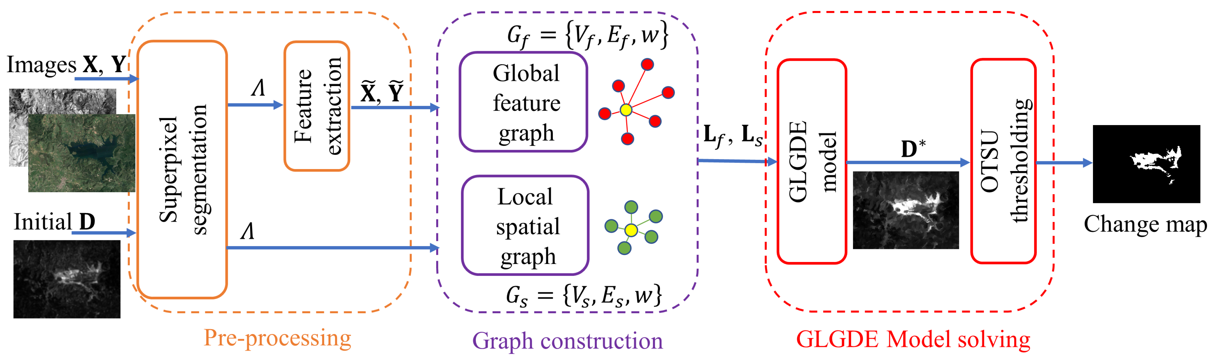
2. Global and Local Graph-Based DI Enhancement
2.1. Pre-Processing
2.2. Global Feature Graph
2.3. Local Spatial Graph
2.4. GLGDE Model
| Algorithm 1: GLGDE-based CD. |
| Input: Images of and , initial DI of . |
| Parameters of , , and . |
| Pre-processing: |
| Segment , , and into superpixels with GMMSP. |
| Extract the features to obtain and . |
| Graph construction: |
| Find the KNN sets of and . |
| Find the R-adjacent neighbors of . |
| Construct the graphs of and . |
| Model solving: |
| Compute the by using (14). |
| Compute the by using (15). |
| Compute final CM by using OTSU thresholding method. |
3. Experimental Results and Discussions
3.1. Experimental Settings
3.2. Experimental Results
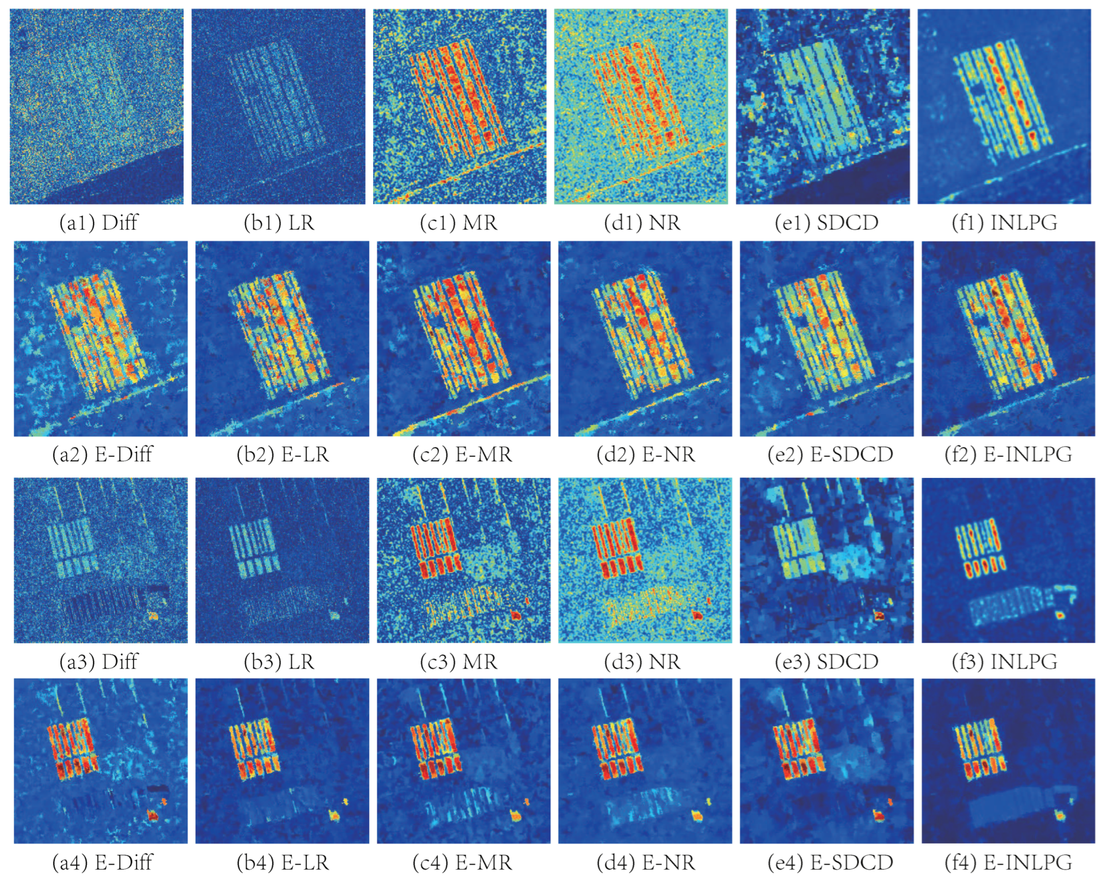
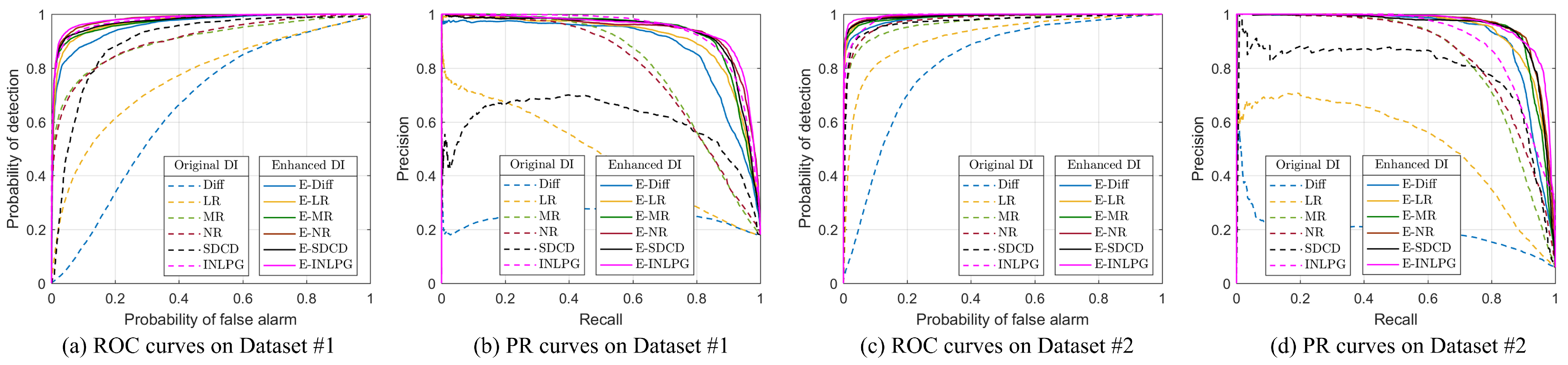
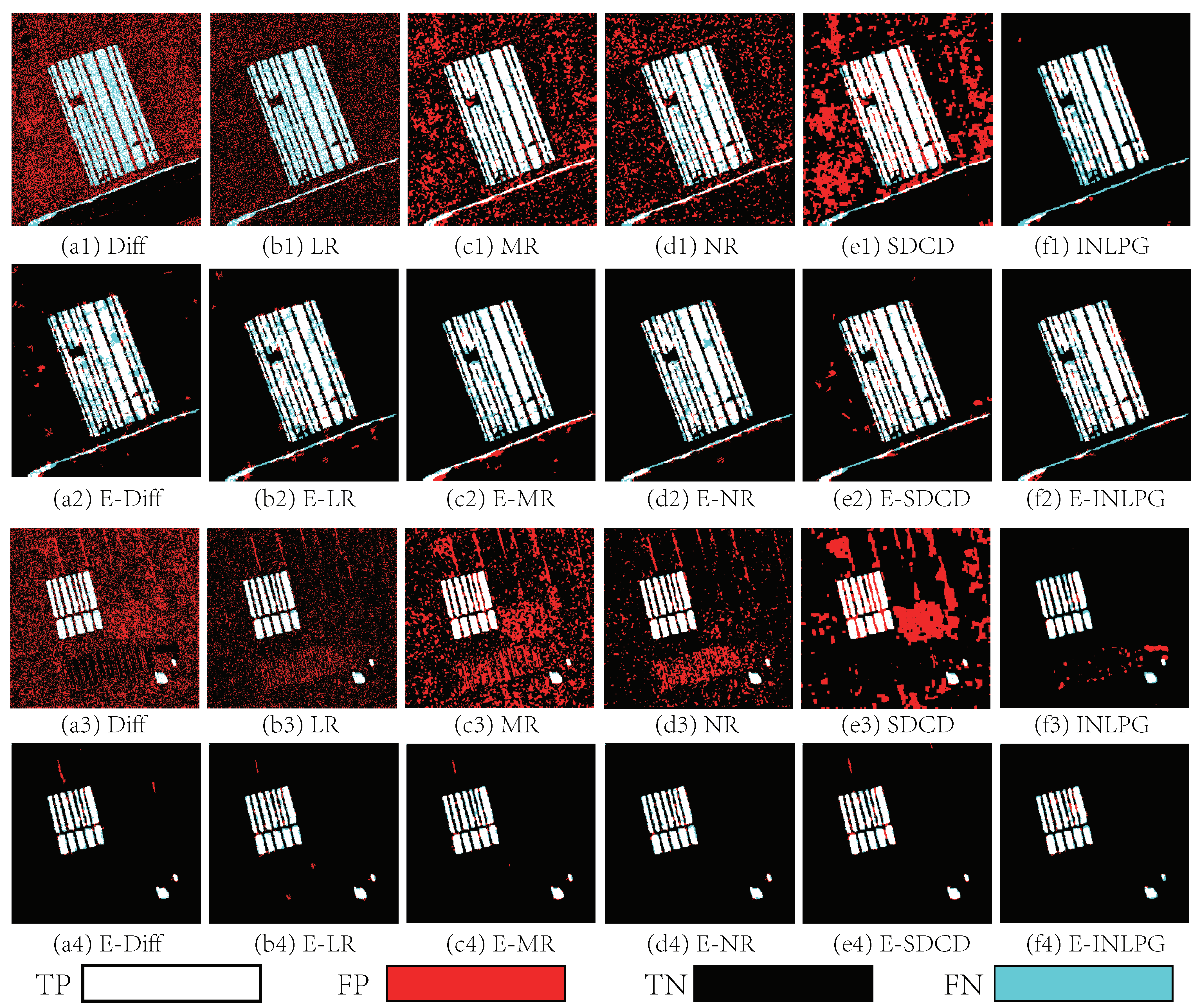
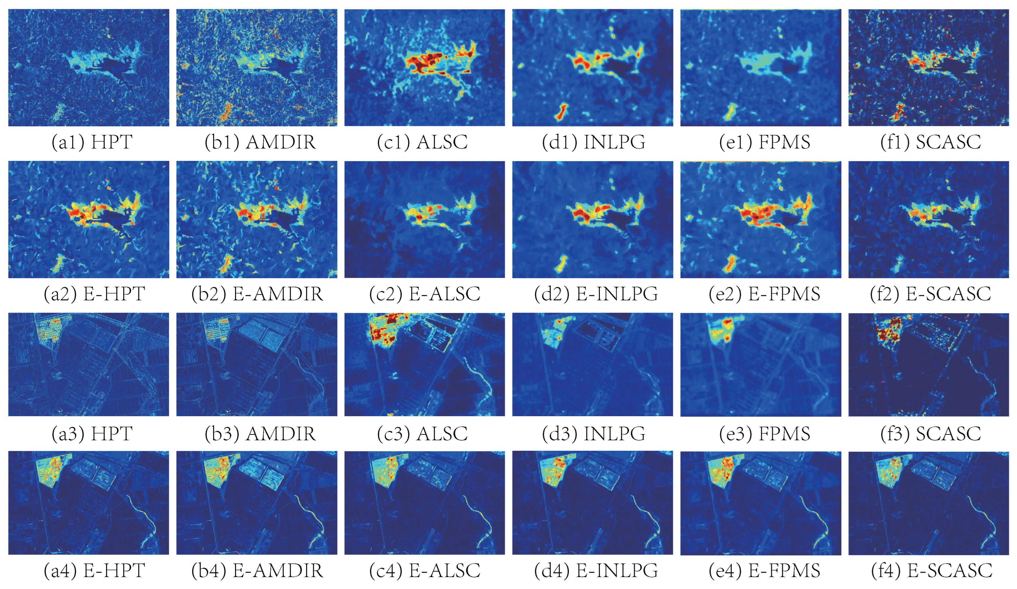
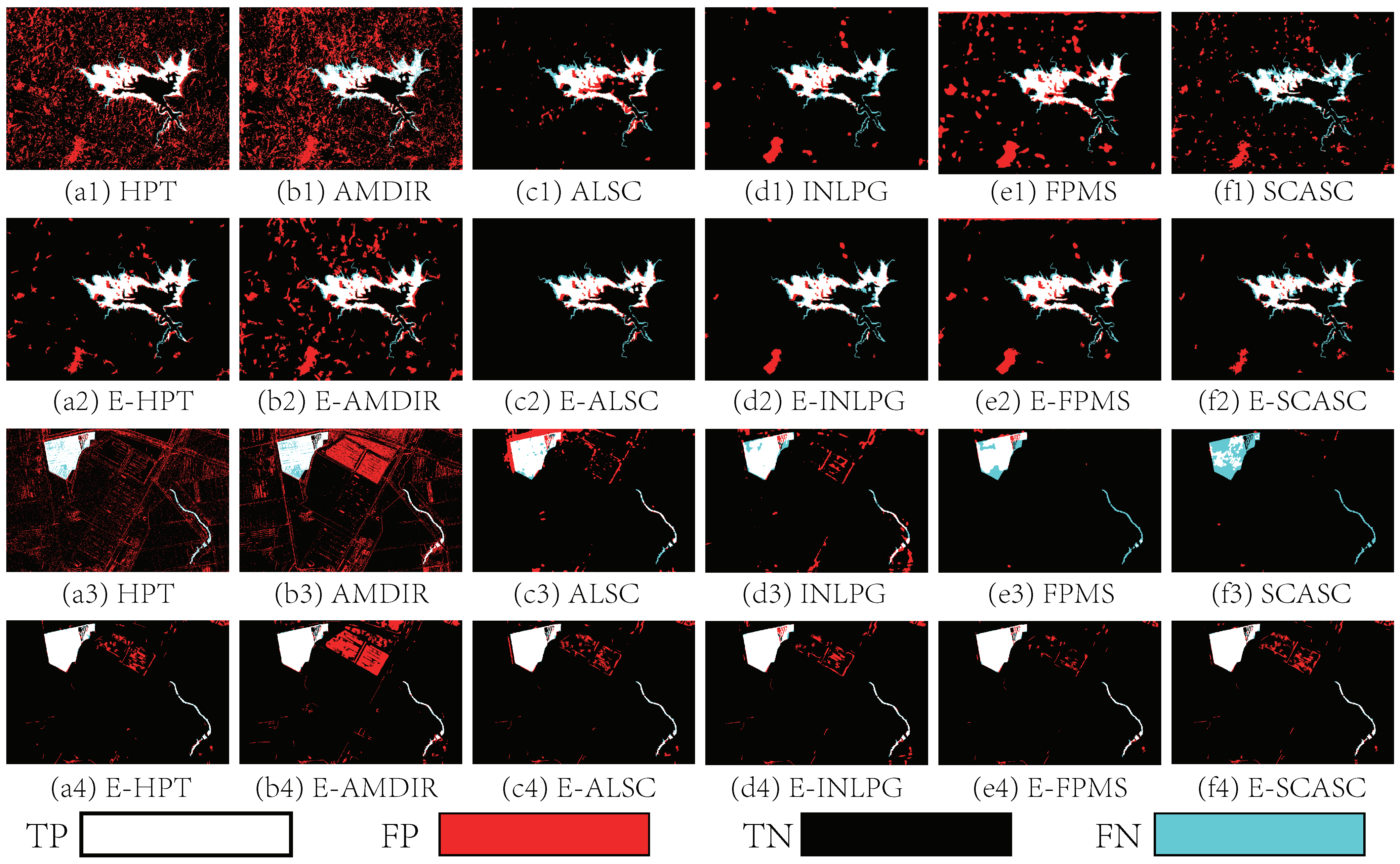
3.2.1. Homogeneous CD of SAR Images
3.2.2. Homogeneous CD of Optical Images
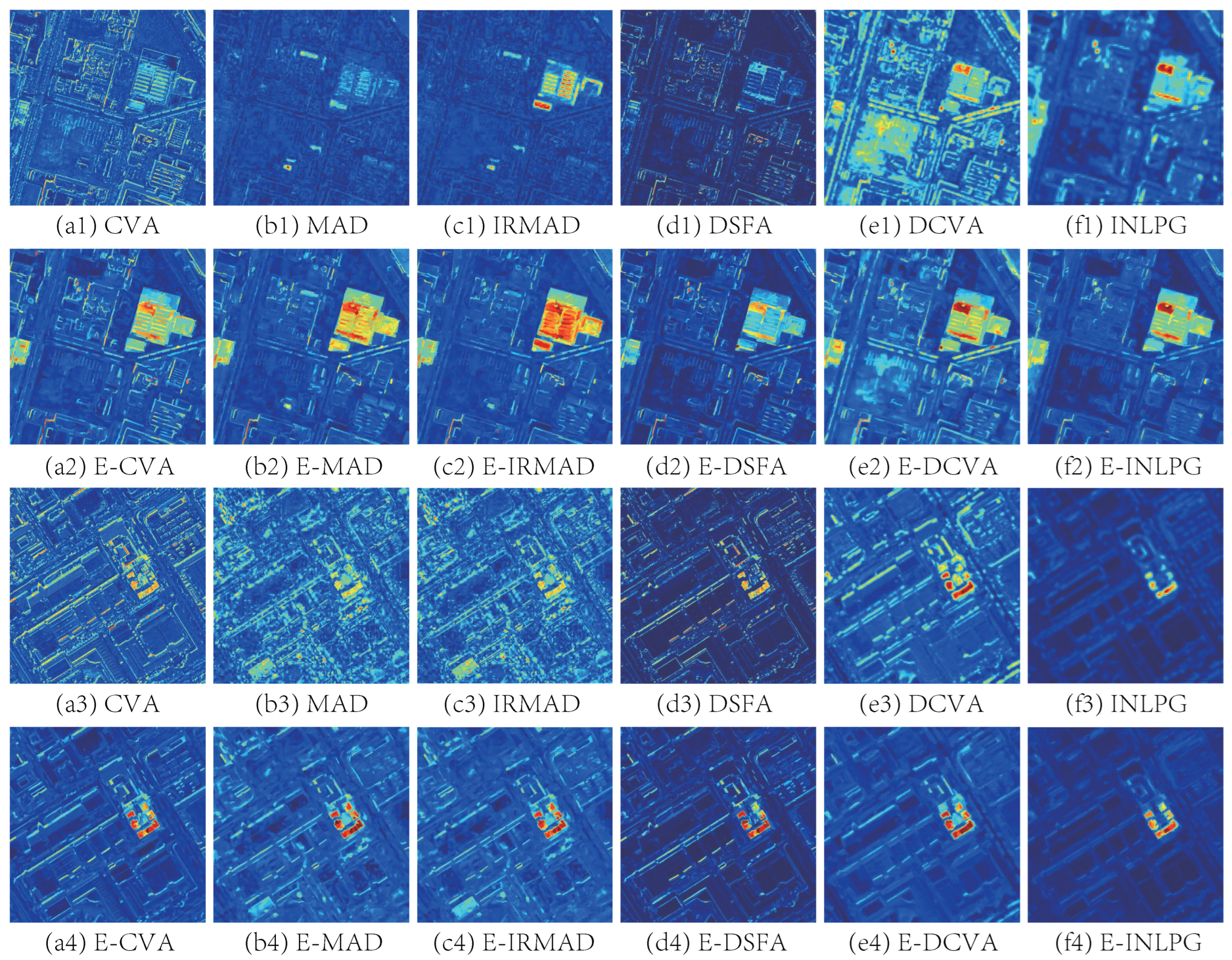
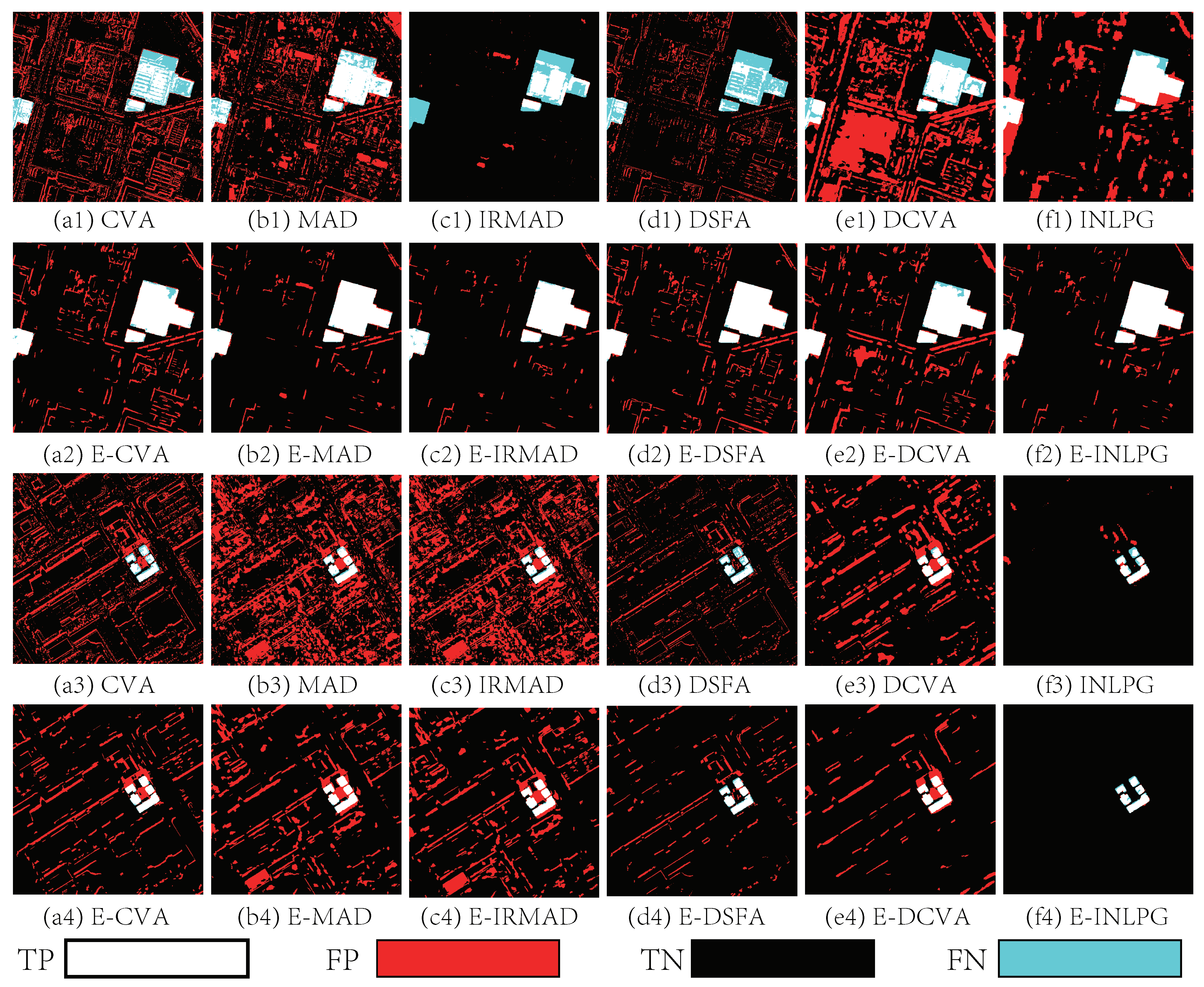
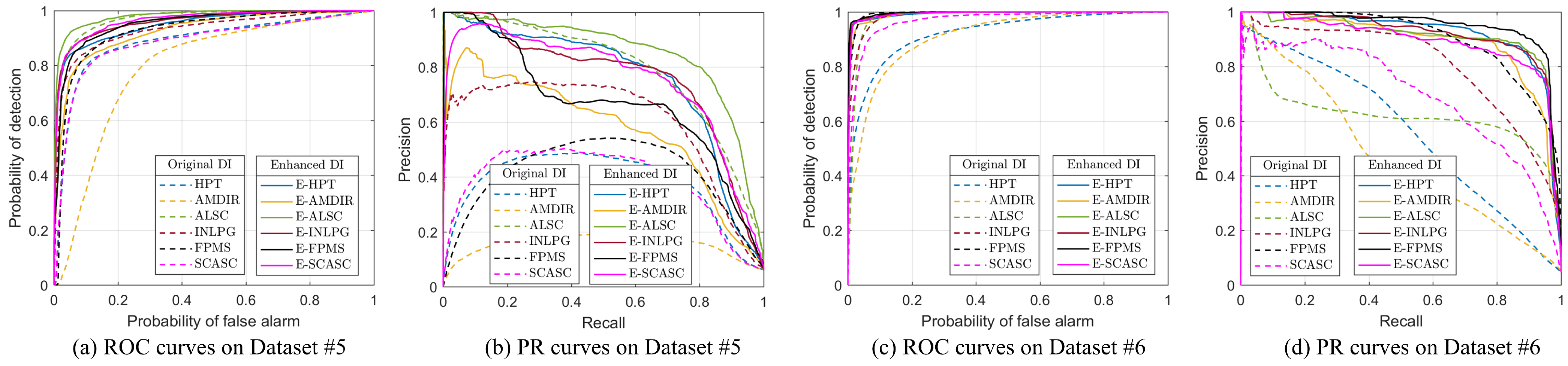
3.2.3. Heterogeneous CD
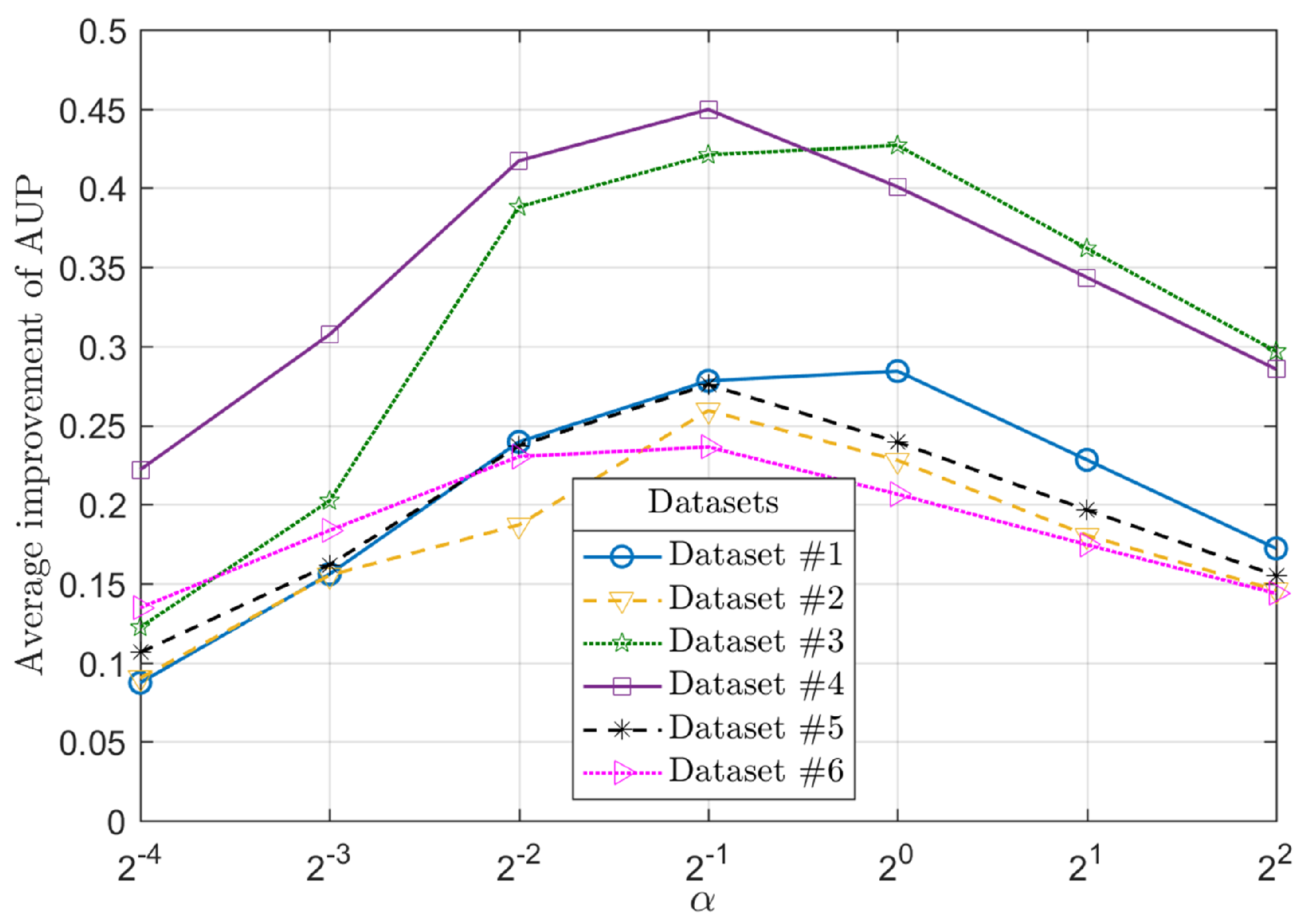
3.3. Parameter Analysis
4. Conclusions
Author Contributions
Funding
Data Availability Statement
Conflicts of Interest
References
- Singh, A. Review Article Digital change detection techniques using remotely-sensed data. Int. J. Remote Sens. 1989, 10, 989–1003. [Google Scholar] [CrossRef]
- Bovolo, F.; Bruzzone, L. The time variable in data fusion: A change detection perspective. IEEE Geosci. Remote Sens. Mag. 2015, 3, 8–26. [Google Scholar] [CrossRef]
- Kennedy, R.E.; Townsend, P.A.; Gross, J.E.; Cohen, W.B.; Bolstad, P.; Wang, Y.; Adams, P. Remote sensing change detection tools for natural resource managers: Understanding concepts and tradeoffs in the design of landscape monitoring projects. Remote Sens. Environ. 2009, 113, 1382–1396. [Google Scholar] [CrossRef]
- Gil-Yepes, J.L.; Ruiz, L.A.; Recio, J.A.; Balaguer-Beser, Á.; Hermosilla, T. Description and validation of a new set of object-based temporal geostatistical features for land-use/land-cover change detection. ISPRS J. Photogramm. Remote Sens. 2016, 121, 77–91. [Google Scholar] [CrossRef]
- Taubenböck, H.; Esch, T.; Felbier, A.; Wiesner, M.; Roth, A.; Dech, S. Monitoring urbanization in mega cities from space. Remote Sens. Environ. 2012, 117, 162–176. [Google Scholar] [CrossRef]
- Zhang, P.; Ban, Y.; Nascetti, A. Learning U-Net without forgetting for near real-time wildfire monitoring by the fusion of SAR and optical time series. Remote Sens. Environ. 2021, 261, 112467. [Google Scholar] [CrossRef]
- Lv, Z.; Liu, T.; Benediktsson, J.A.; Falco, N. Land Cover Change Detection Techniques: Very-high-resolution optical images: A review. IEEE Geosci. Remote Sens. Mag. 2022, 10, 44–63. [Google Scholar] [CrossRef]
- You, Y.; Cao, J.; Zhou, W. A survey of change detection methods based on remote sensing images for multi-source and multi-objective scenarios. Remote Sens. 2020, 12, 2460. [Google Scholar] [CrossRef]
- Shafique, A.; Cao, G.; Khan, Z.; Asad, M.; Aslam, M. Deep learning-based change detection in remote sensing images: A review. Remote Sens. 2022, 14, 871. [Google Scholar] [CrossRef]
- Shi, W.; Zhang, M.; Zhang, R.; Chen, S.; Zhan, Z. Change detection based on artificial intelligence: State-of-the-art and challenges. Remote Sens. 2020, 12, 1688. [Google Scholar] [CrossRef]
- Sun, Y.; Lei, L.; Li, X.; Tan, X.; Kuang, G. Structure Consistency-Based Graph for Unsupervised Change Detection with Homogeneous and Heterogeneous Remote Sensing Images. IEEE Trans. Geosci. Remote Sens. 2022, 60, 4700221. [Google Scholar] [CrossRef]
- Bruzzone, L.; Prieto, D. An adaptive semiparametric and context-based approach to unsupervised change detection in multitemporal remote-sensing images. IEEE Trans. Image Process. 2002, 11, 452–466. [Google Scholar] [CrossRef]
- Liu, Z.; Li, G.; Mercier, G.; He, Y.; Pan, Q. Change Detection in Heterogenous Remote Sensing Images via Homogeneous Pixel Transformation. IEEE Trans. Image Process. 2018, 27, 1822–1834. [Google Scholar] [CrossRef]
- Luppino, L.T.; Bianchi, F.M.; Moser, G.; Anfinsen, S.N. Unsupervised Image Regression for Heterogeneous Change Detection. IEEE Trans. Geosci. Remote Sens. 2019, 57, 9960–9975. [Google Scholar] [CrossRef]
- Lv, Z.; Wang, F.; Liu, T.; Kong, X.; Benediktsson, J.A. Novel Automatic Approach for Land Cover Change Detection by Using VHR Remote Sensing Images. IEEE Geosci. Remote Sens. Lett. 2022, 19, 1–5. [Google Scholar] [CrossRef]
- Luppino, L.T.; Hansen, M.A.; Kampffmeyer, M.; Bianchi, F.M.; Moser, G.; Jenssen, R.; Anfinsen, S.N. Code-Aligned Autoencoders for Unsupervised Change Detection in Multimodal Remote Sensing Images. IEEE Trans. Neural Netw. Learn. Syst. 2022, 1–13. [Google Scholar] [CrossRef] [PubMed]
- Luppino, L.T.; Kampffmeyer, M.; Bianchi, F.M.; Moser, G.; Serpico, S.B.; Jenssen, R.; Anfinsen, S.N. Deep Image Translation with an Affinity-Based Change Prior for Unsupervised Multimodal Change Detection. IEEE Trans. Geosci. Remote Sens. 2022, 60, 4700422. [Google Scholar] [CrossRef]
- Malila, W.A. Change vector analysis: An approach for detecting forest changes with Landsat. In Proceedings of the LARS Symposia, West Lafayette, IN, USA, 3–6 June 1980; p. 385. [Google Scholar]
- Nielsen, A.A.; Conradsen, K.; Simpson, J.J. Multivariate alteration detection (MAD) and MAF postprocessing in multispectral, bitemporal image data: New approaches to change detection studies. Remote Sens. Environ. 1998, 64, 1–19. [Google Scholar] [CrossRef]
- Nielsen, A.A. The Regularized Iteratively Reweighted MAD Method for Change Detection in Multi- and Hyperspectral Data. IEEE Trans. Image Process. 2007, 16, 463–478. [Google Scholar] [CrossRef]
- Saha, S.; Bovolo, F.; Bruzzone, L. Unsupervised Deep Change Vector Analysis for Multiple-Change Detection in VHR Images. IEEE Trans. Geosci. Remote Sens. 2019, 57, 3677–3693. [Google Scholar] [CrossRef]
- Wu, C.; Du, B.; Zhang, L. Slow Feature Analysis for Change Detection in Multispectral Imagery. IEEE Trans. Geosci. Remote Sens. 2014, 52, 2858–2874. [Google Scholar] [CrossRef]
- Du, B.; Ru, L.; Wu, C.; Zhang, L. Unsupervised Deep Slow Feature Analysis for Change Detection in Multi-Temporal Remote Sensing Images. IEEE Trans. Geosci. Remote Sens. 2019, 57, 9976–9992. [Google Scholar] [CrossRef]
- Moser, G.; Serpico, S. Generalized minimum-error thresholding for unsupervised change detection from SAR amplitude imagery. IEEE Trans. Geosci. Remote Sens. 2006, 44, 2972–2982. [Google Scholar] [CrossRef]
- Bovolo, F.; Bruzzone, L. A detail-preserving scale-driven approach to change detection in multitemporal SAR images. IEEE Trans. Geosci. Remote Sens. 2005, 43, 2963–2972. [Google Scholar] [CrossRef]
- Inglada, J.; Mercier, G. A New Statistical Similarity Measure for Change Detection in Multitemporal SAR Images and Its Extension to Multiscale Change Analysis. IEEE Trans. Geosci. Remote Sens. 2007, 45, 1432–1445. [Google Scholar] [CrossRef]
- Nar, F.; Özgür, A.; Saran, A.N. Sparsity-Driven Change Detection in Multitemporal SAR Images. IEEE Geosci. Remote Sens. Lett. 2016, 13, 1032–1036. [Google Scholar] [CrossRef]
- Sun, Y.; Lei, L.; Guan, D.; Li, X.; Kuang, G. SAR Image Change Detection Based on Nonlocal Low-Rank Model and Two-Level Clustering. IEEE J. Sel. Top. Appl. Earth Obs. Remote Sens. 2020, 13, 293–306. [Google Scholar] [CrossRef]
- Zhang, W.; Jiao, L.; Liu, F.; Yang, S.; Liu, J. Adaptive Contourlet Fusion Clustering for SAR Image Change Detection. IEEE Trans. Image Process. 2022, 31, 2295–2308. [Google Scholar] [CrossRef] [PubMed]
- Wang, J.; Zhao, T.; Jiang, X.; Lan, K. A Hierarchical Heterogeneous Graph for Unsupervised SAR Image Change Detection. IEEE Geosci. Remote. Sens. Lett. 2022, 19, 4516605. [Google Scholar] [CrossRef]
- Planinšič, P.; Gleich, D. Temporal Change Detection in SAR Images Using Log Cumulants and Stacked Autoencoder. IEEE Geosci. Remote Sens. Lett. 2018, 15, 297–301. [Google Scholar] [CrossRef]
- Zhang, X.; Su, X.; Yuan, Q.; Wang, Q. Spatial–Temporal Gray-Level Co-Occurrence Aware CNN for SAR Image Change Detection. IEEE Geosci. Remote Sens. Lett. 2022, 19, 4018605. [Google Scholar] [CrossRef]
- Wang, R.; Wang, L.; Wei, X.; Chen, J.W.; Jiao, L. Dynamic Graph-Level Neural Network for SAR Image Change Detection. IEEE Geosci. Remote Sens. Lett. 2022, 19, 4501005. [Google Scholar] [CrossRef]
- Mignotte, M. A Fractal Projection and Markovian Segmentation-Based Approach for Multimodal Change Detection. IEEE Trans. Geosci. Remote Sens. 2020, 58, 8046–8058. [Google Scholar] [CrossRef]
- Sun, Y.; Lei, L.; Guan, D.; Wu, J.; Kuang, G.; Liu, L. Image Regression with Structure Cycle Consistency for Heterogeneous Change Detection. IEEE Trans. Neural Netw. Learn. Syst. 2022, 1–15. [Google Scholar] [CrossRef]
- Sun, Y.; Lei, L.; Tan, X.; Guan, D.; Wu, J.; Kuang, G. Structured graph based image regression for unsupervised multimodal change detection. ISPRS J. Photogramm. Remote Sens. 2022, 185, 16–31. [Google Scholar] [CrossRef]
- Sun, Y.; Lei, L.; Guan, D.; Li, M.; Kuang, G. Sparse-Constrained Adaptive Structure Consistency-Based Unsupervised Image Regression for Heterogeneous Remote-Sensing Change Detection. IEEE Trans. Geosci. Remote Sens. 2022, 60, 4405814. [Google Scholar] [CrossRef]
- Sun, Y.; Lei, L.; Guan, D.; Kuang, G. Iterative Robust Graph for Unsupervised Change Detection of Heterogeneous Remote Sensing Images. IEEE Trans. Image Process. 2021, 30, 6277–6291. [Google Scholar] [CrossRef]
- Sun, Y.; Lei, L.; Li, X.; Sun, H.; Kuang, G. Nonlocal patch similarity based heterogeneous remote sensing change detection. Pattern Recognit. 2021, 109, 107598. [Google Scholar] [CrossRef]
- Sun, Y.; Lei, L.; Guan, D.; Kuang, G.; Liu, L. Graph Signal Processing for Heterogeneous Change Detection. IEEE Trans. Geosci. Remote Sens. 2022, 60, 4415823. [Google Scholar] [CrossRef]
- Zheng, Y.; Zhang, X.; Hou, B.; Liu, G. Using Combined Difference Image and k -Means Clustering for SAR Image Change Detection. IEEE Geosci. Remote Sens. Lett. 2014, 11, 691–695. [Google Scholar] [CrossRef]
- Hou, B.; Wei, Q.; Zheng, Y.; Wang, S. Unsupervised Change Detection in SAR Image Based on Gauss–Log Ratio Image Fusion and Compressed Projection. IEEE J. Sel. Top. Appl. Earth Obs. Remote Sens. 2014, 7, 3297–3317. [Google Scholar] [CrossRef]
- Krähenbühl, P.; Koltun, V. Efficient inference in fully connected crfs with gaussian edge potentials. In Proceedings of the 21st Annual Conference on Neural Information Processing Systems, Granada, Spain, 12–17 December 2011. [Google Scholar]
- Zhang, X.; Su, H.; Zhang, C.; Gu, X.; Tan, X.; Atkinson, P.M. Robust unsupervised small area change detection from SAR imagery using deep learning. ISPRS J. Photogramm. Remote Sens. 2021, 173, 79–94. [Google Scholar] [CrossRef]
- Jimenez-Sierra, D.A.; Quintero-Olaya, D.A.; Alvear-Muñoz, J.C.; Benítez-Restrepo, H.D.; Florez-Ospina, J.F.; Chanussot, J. Graph Learning Based on Signal Smoothness Representation for Homogeneous and Heterogeneous Change Detection. IEEE Trans. Geosci. Remote Sens. 2022, 60, 4410416. [Google Scholar] [CrossRef]
- Ban, Z.; Liu, J.; Cao, L. Superpixel Segmentation Using Gaussian Mixture Model. IEEE Trans. Image Process. 2018, 27, 4105–4117. [Google Scholar] [CrossRef] [PubMed]
- Zheng, X.; Guan, D.; Li, B.; Chen, Z.; Li, X. Change Smoothness-Based Signal Decomposition Method for Multimodal Change Detection. IEEE Geosci. Remote Sens. Lett. 2022, 19, 2507605. [Google Scholar] [CrossRef]
- Otsu, N. A threshold selection method from gray-level histograms. IEEE Trans. Syst. Man Cybern. 1979, 9, 62–66. [Google Scholar] [CrossRef]
- Kittler, J.; Illingworth, J. Minimum error thresholding. Pattern Recognit. 1986, 19, 41–47. [Google Scholar] [CrossRef]
- Hartigan, J.A.; Wong, M.A. Algorithm AS 136: A k-means clustering algorithm. J. R. Stat. Soc. Ser. C (Appl. Stat.) 1979, 28, 100–108. [Google Scholar] [CrossRef]
- Bezdek, J.C.; Ehrlich, R.; Full, W. FCM: The fuzzy c-means clustering algorithm. Comput. Geosci. 1984, 10, 191–203. [Google Scholar] [CrossRef]
- Sun, Y.; Lei, L.; Guan, D.; Wu, J.; Kuang, G. Iterative structure transformation and conditional random field based method for unsupervised multimodal change detection. Pattern Recognit. 2022, 131, 108845. [Google Scholar] [CrossRef]
- Gong, M.; Cao, Y.; Wu, Q. A Neighborhood-Based Ratio Approach for Change Detection in SAR Images. IEEE Geosci. Remote Sens. Lett. 2012, 9, 307–311. [Google Scholar] [CrossRef]
- Lei, L.; Sun, Y.; Kuang, G. Adaptive Local Structure Consistency-Based Heterogeneous Remote Sensing Change Detection. IEEE Geosci. Remote Sens. Lett. 2022, 19, 8003905. [Google Scholar] [CrossRef]


| Dataset | Sensor (or Source) | Size (Pixels) | Date | Location | Event (and Spatial Resolution) |
|---|---|---|---|---|---|
| #1 | Radarsat-2/Radarsat-2 | June 2008–June 2009 | Yellow River, China | Farmland irrigation (8 m) | |
| #2 | Radarsat-2/Radarsat-2 | June 2008–June 2009 | Yellow River, China | Farmland irrigation (8 m) | |
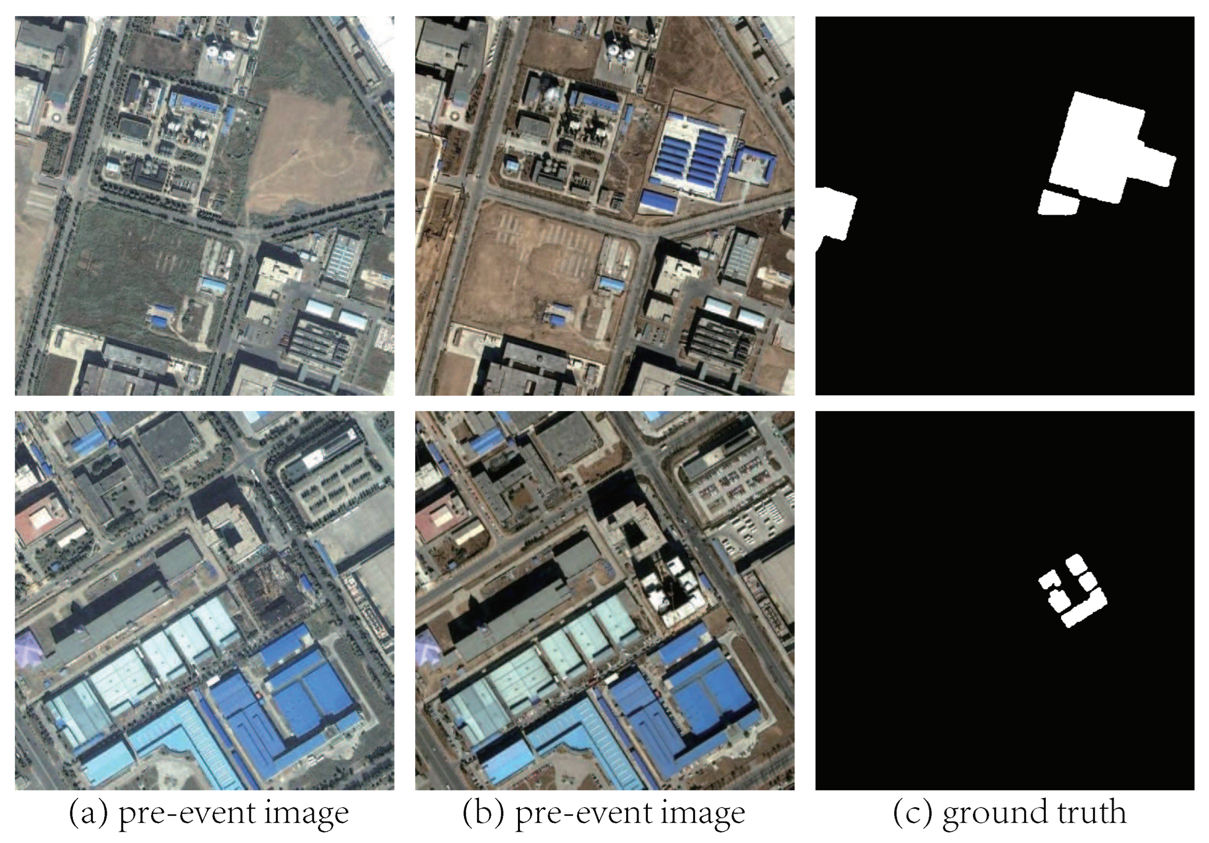
| #3 | Google Earth/Google Earth | September 2012–March 2013 | Beijing, China | Construction (1 m) | |
| #4 | Google Earth/Google Earth | September 2012–March 2013 | Beijing, China | Construction (1 m) | |
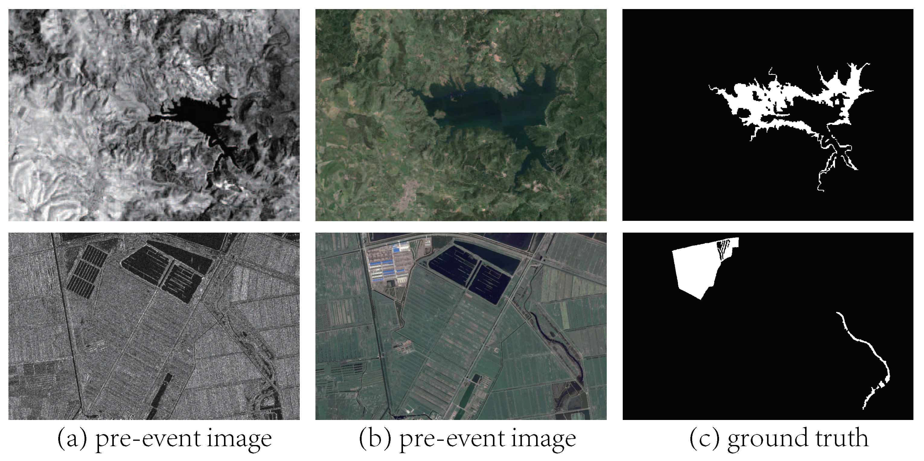
| #5 | Landsat-5/Google Earth | September 1995–July 1996 | Sardinia, Italy | Lake expansion (30 m) | |
| #6 | Radarsat-2/Google Earth | June 2008–September 2012 | Shuguang Village, China | Building construction (8 m) |
| Methods | Dataset #1 | Dataset #2 | ||||||||||
|---|---|---|---|---|---|---|---|---|---|---|---|---|
| AUR ↑ | AUP ↑ | Fa ↓ | Mr ↓ | Oa ↑ | Kc ↑ | AUR ↑ | AUP ↑ | Fa ↓ | Mr ↓ | Oa ↑ | Kc ↑ | |
| Diff | 0.657 | 0.248 | 0.317 | 0.453 | 0.659 | 0.167 | 0.818 | 0.194 | 0.326 | 0.158 | 0.684 | 0.154 |
| LR | 0.764 | 0.478 | 0.185 | 0.404 | 0.775 | 0.351 | 0.916 | 0.525 | 0.143 | 0.156 | 0.856 | 0.352 |
| MR | 0.902 | 0.805 | 0.226 | 0.143 | 0.789 | 0.470 | 0.966 | 0.844 | 0.263 | 0.038 | 0.750 | 0.238 |
| NR | 0.905 | 0.794 | 0.166 | 0.178 | 0.832 | 0.536 | 0.978 | 0.860 | 0.114 | 0.047 | 0.890 | 0.460 |
| SDCD | 0.900 | 0.601 | 0.236 | 0.098 | 0.789 | 0.484 | 0.971 | 0.788 | 0.188 | 0.033 | 0.821 | 0.326 |
| INLPG | 0.978 | 0.938 | 0.008 | 0.264 | 0.946 | 0.798 | 0.990 | 0.909 | 0.013 | 0.163 | 0.978 | 0.809 |
| E-Diff | 0.959 | 0.881 | 0.021 | 0.252 | 0.937 | 0.774 | 0.986 | 0.922 | 0.005 | 0.154 | 0.986 | 0.869 |
| E-LR | 0.971 | 0.911 | 0.017 | 0.228 | 0.945 | 0.802 | 0.993 | 0.943 | 0.005 | 0.172 | 0.985 | 0.863 |
| E-MR | 0.973 | 0.929 | 0.015 | 0.180 | 0.955 | 0.841 | 0.990 | 0.945 | 0.004 | 0.121 | 0.989 | 0.898 |
| E-NR | 0.981 | 0.938 | 0.012 | 0.183 | 0.957 | 0.847 | 0.994 | 0.957 | 0.003 | 0.135 | 0.989 | 0.897 |
| E-SDCD | 0.976 | 0.930 | 0.023 | 0.135 | 0.957 | 0.853 | 0.992 | 0.947 | 0.006 | 0.105 | 0.988 | 0.893 |
| E-INLPG | 0.983 | 0.945 | 0.013 | 0.182 | 0.956 | 0.845 | 0.996 | 0.962 | 0.004 | 0.147 | 0.988 | 0.885 |
| Avg.ipv | 0.123 | 0.278 | −0.173 | −0.063 | 0.153 | 0.359 | 0.052 | 0.259 | −0.170 | 0.040 | 0.157 | 0.494 |
| Methods | Dataset #3 | Dataset #4 | ||||||||||
|---|---|---|---|---|---|---|---|---|---|---|---|---|
| AUR ↑ | AUP ↑ | Fa ↓ | Mr ↓ | Oa ↑ | Kc ↑ | AUR ↑ | AUP ↑ | Fa ↓ | Mr ↓ | Oa ↑ | Kc ↑ | |
| CVA | 0.712 | 0.160 | 0.191 | 0.474 | 0.787 | 0.185 | 0.798 | 0.127 | 0.168 | 0.332 | 0.830 | 0.073 |
| MAD | 0.885 | 0.420 | 0.193 | 0.198 | 0.806 | 0.312 | 0.859 | 0.192 | 0.317 | 0.166 | 0.685 | 0.042 |
| IRMAD | 0.911 | 0.687 | 0.006 | 0.569 | 0.950 | 0.549 | 0.856 | 0.224 | 0.306 | 0.179 | 0.696 | 0.043 |
| DSFA | 0.769 | 0.194 | 0.081 | 0.685 | 0.871 | 0.207 | 0.824 | 0.180 | 0.082 | 0.395 | 0.913 | 0.139 |
| DCVA | 0.715 | 0.212 | 0.335 | 0.329 | 0.666 | 0.127 | 0.955 | 0.614 | 0.140 | 0.095 | 0.860 | 0.127 |
| INLPG | 0.955 | 0.652 | 0.124 | 0.086 | 0.879 | 0.484 | 0.992 | 0.796 | 0.007 | 0.228 | 0.990 | 0.674 |
| E-CVA | 0.975 | 0.685 | 0.076 | 0.047 | 0.926 | 0.631 | 0.978 | 0.706 | 0.093 | 0.066 | 0.907 | 0.195 |
| E-MAD | 0.993 | 0.902 | 0.033 | 0.016 | 0.969 | 0.815 | 0.982 | 0.809 | 0.137 | 0.028 | 0.865 | 0.142 |
| E-IRMAD | 0.995 | 0.942 | 0.022 | 0.035 | 0.977 | 0.858 | 0.980 | 0.799 | 0.140 | 0.033 | 0.861 | 0.137 |
| E-DSFA | 0.976 | 0.680 | 0.073 | 0.018 | 0.932 | 0.658 | 0.979 | 0.702 | 0.047 | 0.160 | 0.952 | 0.306 |
| E-DCVA | 0.975 | 0.744 | 0.093 | 0.049 | 0.911 | 0.580 | 0.994 | 0.867 | 0.050 | 0.036 | 0.950 | 0.328 |
| E-INLPG | 0.992 | 0.898 | 0.035 | 0.012 | 0.966 | 0.804 | 0.999 | 0.949 | 0.001 | 0.194 | 0.997 | 0.876 |
| Avg.ipv | 0.160 | 0.421 | −0.100 | −0.361 | 0.120 | 0.414 | 0.105 | 0.450 | −0.092 | −0.146 | 0.093 | 0.148 |
| Methods | Dataset #5 | Dataset #6 | ||||||||||
|---|---|---|---|---|---|---|---|---|---|---|---|---|
| AUR ↑ | AUP ↑ | Fa ↓ | Mr ↓ | Oa ↑ | Kc ↑ | AUR ↑ | AUP ↑ | Fa ↓ | Mr ↓ | Oa ↑ | Kc ↑ | |
| HPT | 0.889 | 0.373 | 0.196 | 0.138 | 0.808 | 0.286 | 0.922 | 0.564 | 0.117 | 0.181 | 0.880 | 0.339 |
| AMDIR | 0.795 | 0.155 | 0.224 | 0.277 | 0.773 | 0.203 | 0.911 | 0.470 | 0.151 | 0.180 | 0.848 | 0.279 |
| ALSC | 0.972 | 0.793 | 0.026 | 0.218 | 0.962 | 0.696 | 0.980 | 0.623 | 0.038 | 0.115 | 0.958 | 0.641 |
| INLPG | 0.930 | 0.604 | 0.027 | 0.297 | 0.956 | 0.642 | 0.985 | 0.808 | 0.029 | 0.151 | 0.965 | 0.672 |
| FPMS | 0.925 | 0.406 | 0.083 | 0.189 | 0.911 | 0.486 | 0.994 | 0.904 | 0.004 | 0.310 | 0.982 | 0.768 |
| SCASC | 0.885 | 0.383 | 0.043 | 0.420 | 0.934 | 0.485 | 0.968 | 0.695 | 0.002 | 0.713 | 0.965 | 0.418 |
| E-HPT | 0.948 | 0.757 | 0.035 | 0.186 | 0.956 | 0.672 | 0.992 | 0.922 | 0.019 | 0.044 | 0.979 | 0.800 |
| E-AMDIR | 0.926 | 0.576 | 0.092 | 0.181 | 0.903 | 0.465 | 0.991 | 0.889 | 0.060 | 0.039 | 0.941 | 0.571 |
| E-ALSC | 0.980 | 0.851 | 0.011 | 0.229 | 0.975 | 0.781 | 0.994 | 0.911 | 0.021 | 0.040 | 0.979 | 0.794 |
| E-INLPG | 0.959 | 0.761 | 0.017 | 0.261 | 0.968 | 0.723 | 0.994 | 0.920 | 0.020 | 0.038 | 0.980 | 0.802 |
| E-FPMS | 0.953 | 0.669 | 0.040 | 0.221 | 0.949 | 0.626 | 0.996 | 0.948 | 0.011 | 0.039 | 0.987 | 0.869 |
| E-SCASC | 0.964 | 0.755 | 0.018 | 0.280 | 0.966 | 0.705 | 0.992 | 0.892 | 0.021 | 0.038 | 0.978 | 0.792 |
| Avg.ipv | 0.056 | 0.276 | −0.064 | −0.030 | 0.062 | 0.196 | 0.033 | 0.236 | −0.032 | −0.235 | 0.041 | 0.252 |
Disclaimer/Publisher’s Note: The statements, opinions and data contained in all publications are solely those of the individual author(s) and contributor(s) and not of MDPI and/or the editor(s). MDPI and/or the editor(s) disclaim responsibility for any injury to people or property resulting from any ideas, methods, instructions or products referred to in the content. |
© 2023 by the authors. Licensee MDPI, Basel, Switzerland. This article is an open access article distributed under the terms and conditions of the Creative Commons Attribution (CC BY) license (https://creativecommons.org/licenses/by/4.0/).
Share and Cite
Zheng, X.; Guan, D.; Li, B.; Chen, Z.; Pan, L. Global and Local Graph-Based Difference Image Enhancement for Change Detection. Remote Sens. 2023, 15, 1194. https://doi.org/10.3390/rs15051194
Zheng X, Guan D, Li B, Chen Z, Pan L. Global and Local Graph-Based Difference Image Enhancement for Change Detection. Remote Sensing. 2023; 15(5):1194. https://doi.org/10.3390/rs15051194
Chicago/Turabian StyleZheng, Xiaolong, Dongdong Guan, Bangjie Li, Zhengsheng Chen, and Lefei Pan. 2023. "Global and Local Graph-Based Difference Image Enhancement for Change Detection" Remote Sensing 15, no. 5: 1194. https://doi.org/10.3390/rs15051194
APA StyleZheng, X., Guan, D., Li, B., Chen, Z., & Pan, L. (2023). Global and Local Graph-Based Difference Image Enhancement for Change Detection. Remote Sensing, 15(5), 1194. https://doi.org/10.3390/rs15051194