Article

Multi-Scale Feature Interaction Network for Remote Sensing Change Detection

1
Collaborative Innovation Center on Atmospheric Environment and Equipment Technology, Nanjing University of Information Science and Technology, Nanjing 210044, China
2
College of Information Science and Technology, Nanjing Forestry University, Nanjing 210044, China
*
Author to whom correspondence should be addressed.
Remote Sens. 2023, 15(11), 2880; https://doi.org/10.3390/rs15112880
Submission received: 28 March 2023 / Revised: 22 May 2023 / Accepted: 29 May 2023 / Published: 1 June 2023

Abstract

:
Change detection (CD) is an important remote sensing (RS) data analysis technology. Existing remote sensing change detection (RS-CD) technologies cannot fully consider situations where pixels between bitemporal images do not correspond well on a one-to-one basis due to factors such as seasonal changes and lighting conditions. Existing networks construct two identical feature extraction branches through convolution, which share weights. The two branches work independently and do not merge until the feature mapping is sent to the decoder head. This results in a lack of feature information interaction between the two images. So, directing attention to the change area is of research interest. In complex backgrounds, the loss of edge details is very important. Therefore, this paper proposes a new CD algorithm that extracts multi-scale feature information through the backbone network in the coding stage. According to the task characteristics of CD, two submodules (the Feature Interaction Module and Detail Feature Guidance Module) are designed to make the feature information between the bitemporal RS images fully interact. Thus, the edge details are restored to the greatest extent while fully paying attention to the change areas. Finally, in the decoding stage, the feature information of different levels is fully used for fusion and decoding operations. We build a new CD dataset to further verify and test the model’s performance. The generalization and robustness of the model are further verified by using two open datasets. However, due to the relatively simple construction of the model, it cannot handle the task of multi-classification CD well. Therefore, further research on multi-classification CD algorithms is recommended. Moreover, due to the high production cost of CD datasets and the difficulty in obtaining them in practical tasks, future research will look into semi-supervised or unsupervised related CD algorithms.

Graphical Abstract

1. Introduction

In recent years, with the rapid development of RS imaging technology, effectively extracting target change information from remote sensing images has become one of the research goals of academia and industry. Change detection (CD) technology plays an important role in urban change [1,2], agricultural surveys [3,4], and natural disaster assessment [5,6]. However, with the continuous progress of RS technology, the spectral information features or spatial information features of a pair of bitemporal RS images will be very different due to seasonal, lighting, and other factors [7]. Therefore, in such a complex background, traditional manual drawing methods can no longer handle CD tasks. Most existing CD technologies are implemented using computer algorithms to avoid false detection and omissions due to perceptions.
Existing CD algorithms can generally be divided into unsupervised and supervised algorithms. For example, traditional iterative weighted multivariate change detection (IR-MAD) [8] based on k-means clustering and the principal component analysis (PCA) [9] are unsupervised algorithms. They determine whether there is a change by calculating the relationship between the pixels of a dual-time image. However, this detection method is prone to large-scale error detection due to the significant differences in the spectral information characteristics of existing images and the lack of prior data. According to different task scenarios, it is necessary to manually adjust parameters, but this method is time-consuming. Due to the increasingly widespread application of deep learning, convolutional neural networks (CNNs) have been applied in various fields [10,11,12,13,14]. In 2015, Gong et al. [15] proposed using neural networks for RS-CD. In 2017, Zhan et al. [16] proposed a dual convolution divine meridian based on deep learning. In 2018, Varghese et al. [17] created a new network that combines dual convolutional neural network output feature extraction with a full convolutional network (FCN). In 2020, Peng et al. [18] proposed the Counter Network (GAN). In 2021, Chen et al. [19,20,21,22] proposed a dual-time image converter (BIT) based on a converter.
It should be borne in mind that dual-time RS images refer to images taken at different time periods but at the same location. Therefore, due to season, illumination, and other factors, the spectral or spatial information characteristics of the two images are very different, which leads to the challenge of one-to-one pixel matching. This leads to many errors and omission detection, usually caused by the inability to effectively and fully fuse the features extracted from the two images in the original image [23,24]. However, most CD methods are based on CNN during the encoding phase. They use fixed-size convolutions to down-sample feature information and obtain feature information of different scales. Due to the limited acceptance area of a single convolution, it is not possible to extract sufficient context information during the feature extraction phase, which reduces the performance of the model. In addition, existing CD methods also have many shortcomings in feature fusion. Fusion operations are mainly performed at the initial and end stages of coding, without considering feature interactions during the coding process. This fusion method loses a large amount of critical context information during the coding phase [25,26,27], which makes the model unable to learn the feature information of the changing region, resulting in errors and missed detection.
To solve the problem of insufficient feature extraction and fusion, this paper designs a Multi-Scale Feature Interaction Network (MFIN). In the coding stage, the multi-scale feature information in the image is extracted to restore the context feature information to the maximum extent. According to the task characteristics of CD, two auxiliary modules are designed to make the feature information between networks fully interact. The network can learn the feature information of the change area and fully restore the edge details. In the decoding stage, the feature information of different scales is fully used for fusion and decoding. This method reduces the false detection and missed detection caused by insufficient multi-level feature information extraction and fusion.
The main innovations of this paper are as follows: (1) The network proposed in this paper enables end-to-end training without the separate training of submodules. Moreover, in a task scene with complex seasonal lighting, the network can fully extract and fuse multi-level feature information to minimize the occurrence of false detection and missed detection. (2) The task characteristics of CD are fully considered, and the network is designed pertinently. In the coding stage, the designed Multi-Scale Feature Extraction Network (MFEN) and two submodules enable the model to restore the edge details to the maximum extent while fully paying attention to the feature information of the change area, thus improving the model accuracy. (3) A new RS-CD dataset is established, which contains enough kinds of change categories. All data are annotated manually to ensure accuracy. Experiments show that the established dataset is feasible for the quantitative evaluation of CD tasks.
The rest of this paper is organized as follows: Section 2 introduces each network in the model. Section 3 analyzes the composition of the dataset. Section 4 analyzes the performance of the model through experiments. Section 5 summarizes the whole paper and puts forward the future work.

2. Methodology

The Multi-Scale Feature Interaction Network (MFIN) proposed in this paper consists of the following aspect: the backbone Multi-Scale Feature Extraction Network (MFEN), which is used to collect multi-scale features from dual-time RS images. The other two auxiliary modules are the Functional Interaction Module (FIM) and the Detailed Functional Guidance Module (DFGM). FIM makes the model pay more attention to the changed parts, and combining the changed parts greatly improves the accuracy. DFGM further guides the model in learning underlying spatial details without increasing computational costs, thereby making the model pay more attention to edge details. An MLP encoder is designed to fuse and decode multi-scale feature information in the decoding section. The framework of the MFIN is shown in Figure 1.

2.1. Multi-Scale Feature Extraction Network

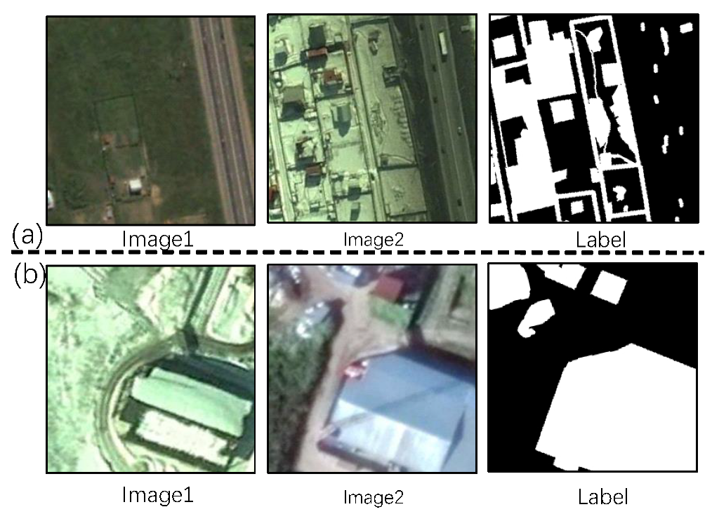
In the RS-CD tasks, the data of the model are dual-time RS images taken at the same location but at different time periods. Therefore, due to factors such as season and illumination, the two images’ spectral or spatial information characteristics differ greatly, and pixels cannot be well matched, as shown in Figure 2. In this case, if the multi-scale feature information cannot be fully extracted in the encoding stage, errors and missed detection may occur due to the correspondence of differences between pixels.
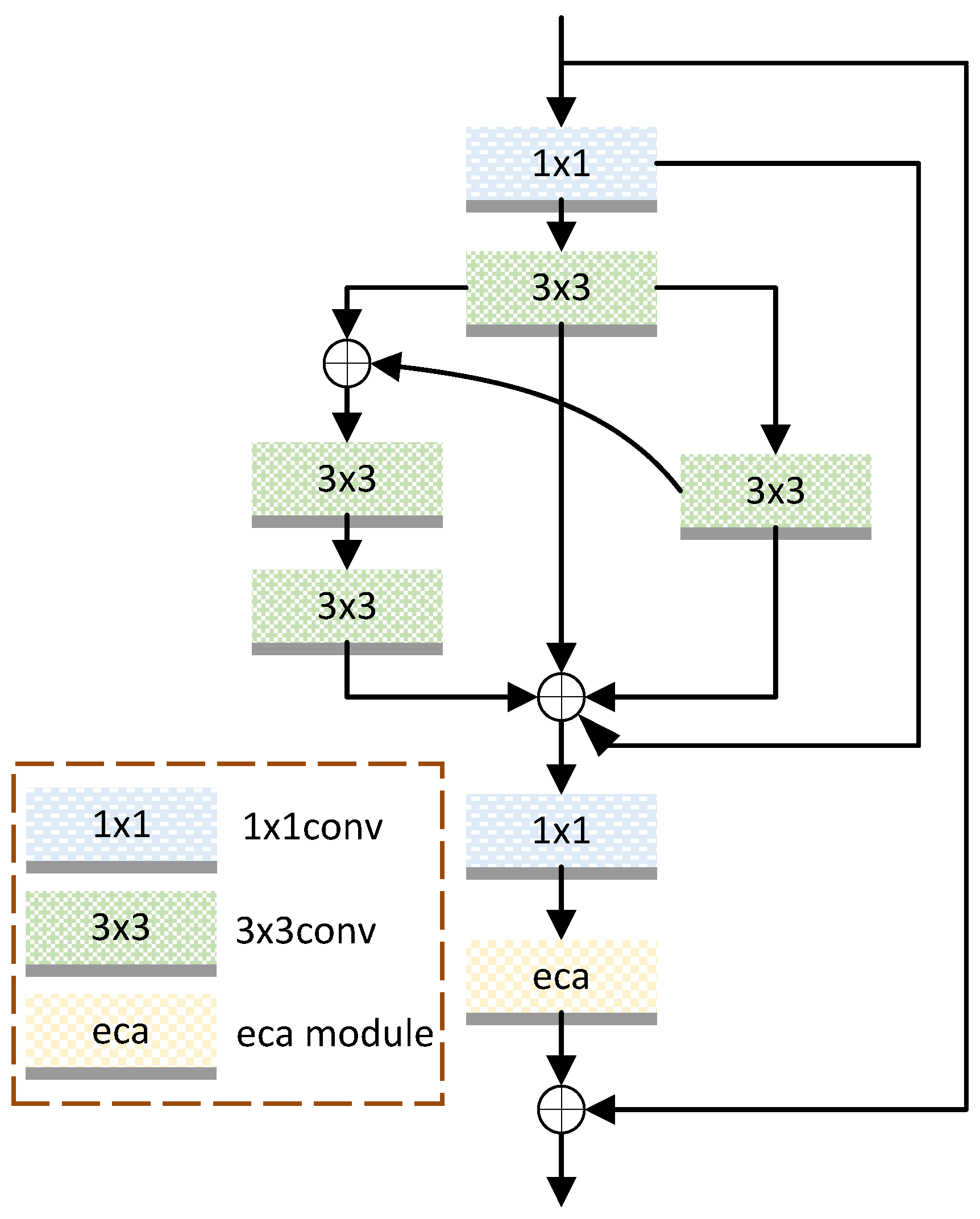
Therefore, given the above situation, this article designs an MFEM (Figure 3). This module is mainly composed of a 1 × 1 convolution and a 3 × 3 convolution. The convolution and effective channel attention module composition (ECA) [28] performs normalization and ReLU activation processing after each convolution core. The specific structure is as follows: We use the 1 × 1 convolution to adjust the channel, and then we use the 3 × 3 convolution. The multi-scale feature information is extracted by the convolution, and the feature information of different scales is fused through an addition operation. Finally, the output after fusion passes the 1 × 1 convolution to recover the number of characteristic channels. The two paths on the far right are quick links.
The core of the MFEM is the 3 × 3 convolution structure, which is conducive to processing objects of different scales in the CD task. Through our unique design structure, the MFEM can gather receptive fields of sizes 3 × 3, 5 × 5, 7 × 7, and 9 × 9, as can be seen in Figure 3. First, the 1 × 1 convolution is passed through for dimension reduction. The right branch passes through two 3 × 3 convolutions to obtain a 5 × 5 convolution. The left branch passes through three 3 × 3 convolutions to yield a 7 × 7 convolution. Namely, four 3 × 3 convolutions result in a 9 × 9 convolution. Finally, information fusion is performed. In the experimental part, the MFEM designed in this paper is compared with other feature extraction networks to further verify its effectiveness.

2.2. Feature Interaction Module

The CD task differs from traditional segmentation and classification tasks in that the detection data are a pair of dual-time data. Therefore, the interaction of feature information between two images can make the network filter out the key feature information. However, most existing CD algorithms build two independent branches to extract the feature information from two images. In addition, most of them do not interact with the feature information of the two images, which makes the model focus on the feature information of the changed part. This feature extraction method without a selection will result in less feature mapping, thus reducing the model performance of the backbone network. With the deepening of the backbone feature extraction network, feature interaction becomes more focused on changing parts of the region.
Therefore, to better determine the change area, we need to interactively process the feature information of the two images. Inspired by the self-attention mechanism, we design the Feature Interaction Module (FIM) (Figure 4). First, we map Feature_1 and Feature_2 to Query, Key, and Value; then, multiplying Query and Key in Feature_1 and Feature_2, respectively, makes the network pay more attention to the feature information of the change region; finally, after the Softmax operation, the output result is summed and output with the original feature. The specific calculation formula is as follows:
X 1 = X 1 + softmax Q 2 × K 1 T d × V 1 ,
X 2 = X 2 + softmax Q 1 × K 2 T d × V 2 ,
where X 1 and X 2 are feature maps, and d is the dimension of matrices Q 1 and Q 2 . Q i , K i , and V i (i = 1, 2) denote the corresponding Query, Key, and Value in X i , respectively.
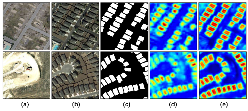
Figure 5 shows the visualization results of FIM. Figure 5a,b present bitemporal remote sensing images of the same area. Figure 5c is its label diagram. Figure 5d,e show heat maps with and without FIM, respectively. We clearly find that, after introducing FIM into the network, the network pays more attention to the pixels in some change areas that it was previously indifferent to or less concerned about. That is the red area in the heat map.

2.3. Detail Feature Guidance Module

Nowadays, the background of RS data is most complex, and the edge detail information is much better than before. Therefore, if only the feature information is extracted from the main network, the detailed points are ignored to a certain extent, which also reduces the accuracy of the network. To solve this problem, we propose a Detail Feature Guidance Module (DFGM) to direct the backbone network to learn the single stream’s detailed feature information. As shown in Figure 1, we create the detail map ground truth using the Laplace operator. Then, we insert the generated detail head into the backbone network to create a detail feature map. Finally, the detailed feature map provides the ground truth to guide the backbone network to learn more detailed information. The details are given below.
The binary detail ground truth is generated by us from the semantically segmented ground truth through the DFGM. This operation can be realized by the 1 × 1 convolution and the 2-D convolution kernel named the Laplacian kernel.
To make the model more accurate, as shown in Figure 1, we generate a detailed map using the detail head, guiding the backbone network to learn the detailed feature information more fully and efficiently. This method can add the representation of features in the training stage and be discarded in the reasoning stage. The detail head contains a Conv-BN-ReLU operator, where the convolution kernel size is 3. Then, there is a 1 × 1 convolution to obtain the output. Through experiments, we verify that the detail head can effectively increase the representation of detail features. In particular, this branch is abandoned in the reasoning stage. Therefore, the information extracted by this module can increase the accuracy of RS-CD tasks easily without any cost in inference. In the actual tasks, the number of pixels corresponding to the detailed feature information is much smaller than that corresponding to the detailed information, so the detailed feature prediction can be treated as a class imbalance problem. If the traditional weighted cross-entry is used, it will be difficult to obtain good results. Therefore, we use binary cross-entropy and the dice loss to mutually optimize detail learning. The overlap between the ground truth and predicted maps is measured by using the dice loss. Moreover, the dice loss is not sensitive to the quantity of foreground and background pixels. So, the dice loss can better deal with the problem of class imbalance. If the forecast detail maps’ height and width are H and W, the detail loss L d is expressed as follows:
L d ( x p d , x d g ) = L b c e ( x p d , x d g ) + L d i c e ( x p d , x d g ) ,
where x p d R H × W represents the predicted detail, and x d g R H × W represents the corresponding detail ground truth. L b c e denotes the binary cross-entropy loss, while L d i c e denotes the dice loss. The calculation result of L d i c e is shown in the following formula:
L d i c e ( x p d , x d g ) = 1 2 i H × W x p d i x d g i + 1 i H × W ( x p d i ) 2 + i H × W ( x d g i ) 2 + 1 .
i represents the i-th pixel. To not divide by 0, set the Laplacian smoothing item to 1.

2.4. MLP Decoder

In the decoding stage, we built the decoder using MLP and upsample. Firstly, the output feature map of each stage in the encoder is processed by MLP to unify the number of channel dimensions, and then the feature map size is uniformly restored to the size of H/2 × W/2 by using the upsample operation. Then, the feature maps processed by each stage are fused and connected by the MLP layer. Finally, the fused feature maps are upsampled to the size of H × W, and the classifier operation is performed. The specific calculation is as follows:
F ¯ i = Upsample ( Linear ( C i , C e b d , F i ) ) ( i = 1 , 2 , 3 , 4 ) ,
F = Linear ( 4 C b e d , C b e d , C at ( F ¯ 1 , F ¯ 2 , F ¯ , 3 , F ¯ 4 ) ) ,
O u t = Linear ( C b e d , n , Upsample ( F ) ) ,
where F i denotes the output feature map of the i-th stage, C e b d denotes the embedding dimension, C i denotes the dimension of the output feature map of the i-th stage, and n is the number of classes.

3. Data Sources

The validation of RS-CD requires a huge amount of data support. However, there are relatively few datasets in this field. Therefore, we created a new dataset, BRSCDD. In addition, the generalization of our network was further verified by using the open dataset LEVIR-CD [29] and CDD [30].

3.1. BRSCDD

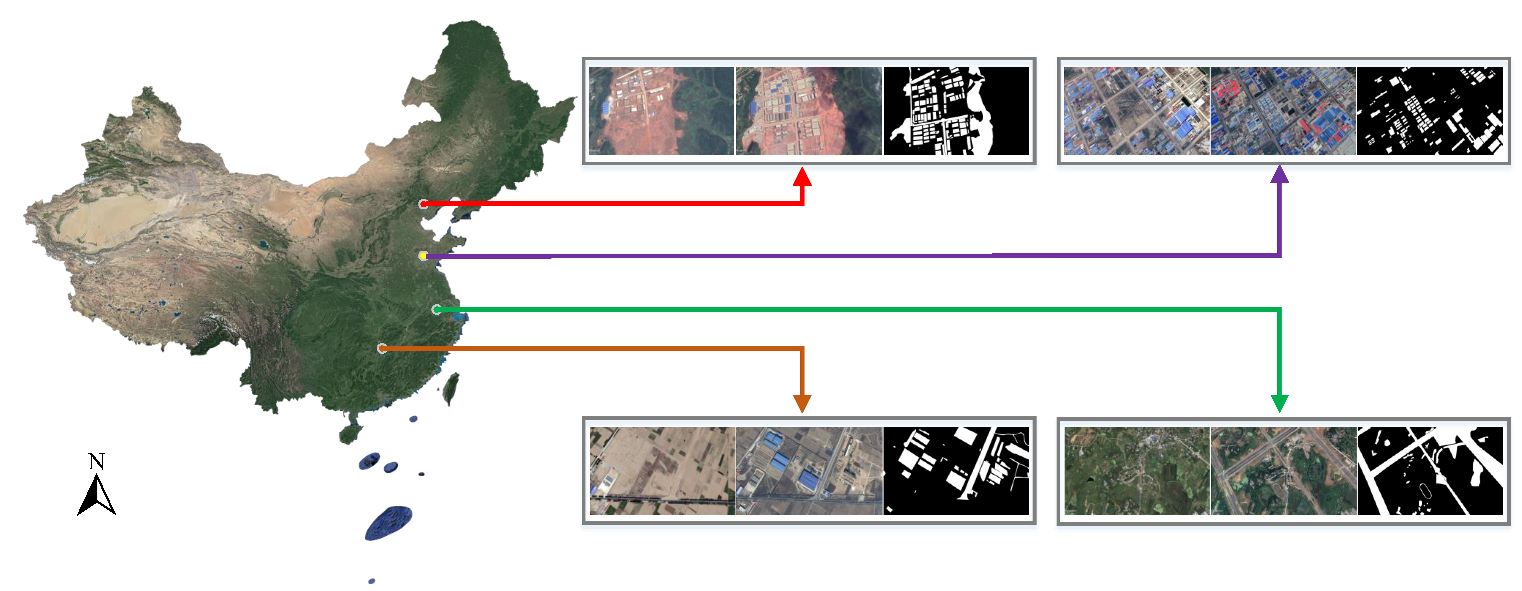
Compared with other published datasets, most of the bitemporal RS images in the dataset used in this work are in central and eastern China, and the observation distance is short, which contains more details of objects and their environment. There are 3600 pairs of bitemporal RS images with a resolution of 512 × 512 , and the corresponding area of each image is about 3 square kilometers. The images of Google Earth (GE) contain photos taken at different times in the same place from 2010 to 2022. GE is a piece of virtual Earth software developed by Google. Through this software, users can view high-definition RS images in different countries, places, and time periods all over the world for free. GE’s satellite images are mainly from Digital Globe’s Quick Bird commercial satellite and the Earth satellite, and the image part is mainly from landsat-7. In terms of resolution and field height, GE’s resolution is usually 30 m, and the field height is usually 15 km. However, for some famous scenic spots, high-precision images with a resolution of 1m or 0.6m should be used, and the viewing height is about 500 m or 350 m, respectively. We collect images of these places in the dataset. Moreover, in the process of collection, we complete the registration of Google Earth’s bitemporal images. We enhance the robustness of the model by covering many objects in the dataset, such as buildings, mining areas, roads, factories, and farmland. We manually label all tags to ensure that the information in the dataset is accurate enough.
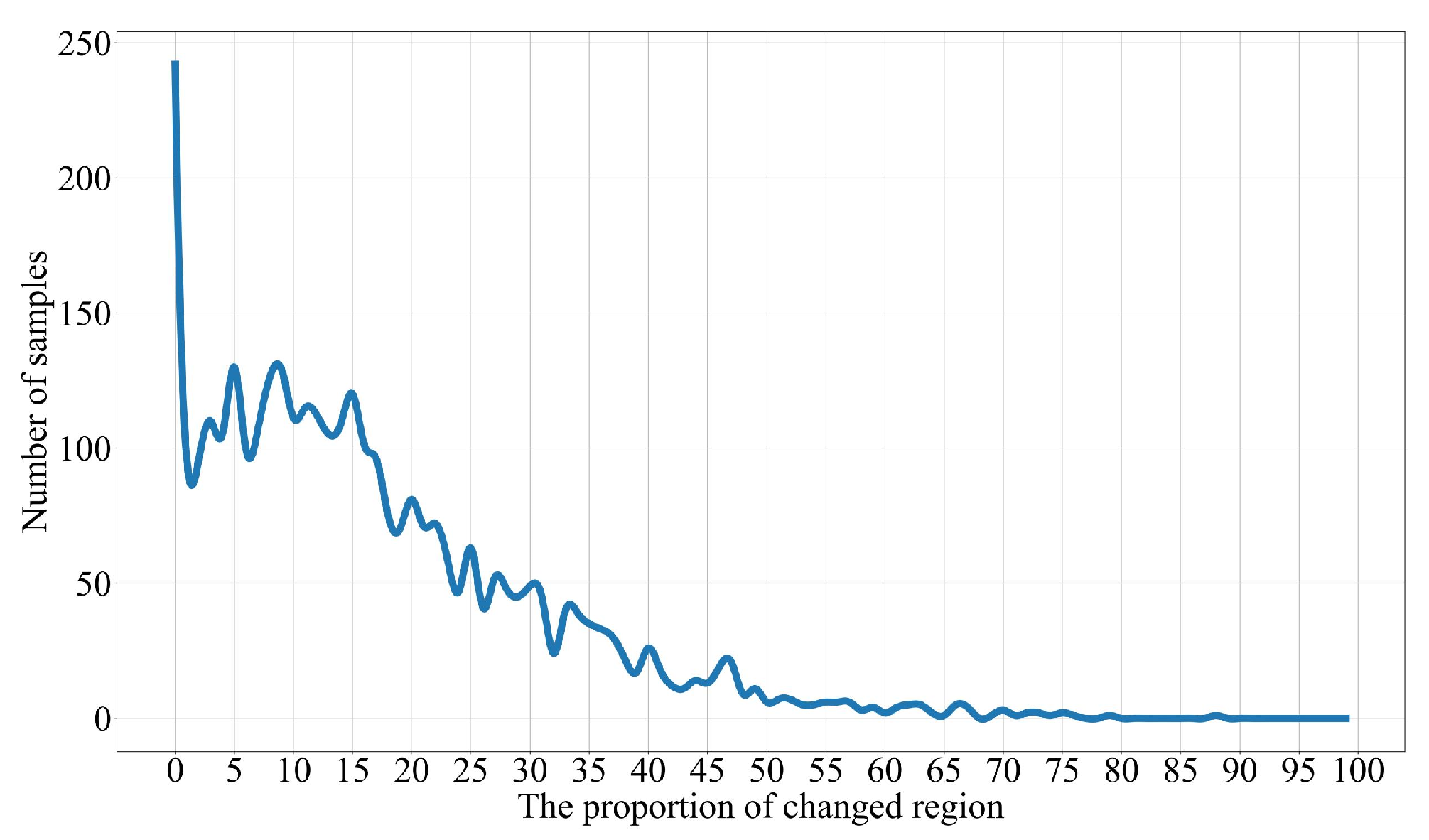
Figure 6 contains many common scenarios in the dataset, such as buildings, roads, and factories. In order to imitate the actual application scenario to a greater extent, we add some additional image pairs in the dataset, such as some images with large shooting angle deviations. Figure 7 shows a statistical analysis of the dataset, in which the change area of most of the sample data is between 5% and 50%. There are 247 samples with a change area ratio of 0–2%. By increasing the imbalance between the samples, the performance of the model can be better tested.

3.2. LEVIR-CD

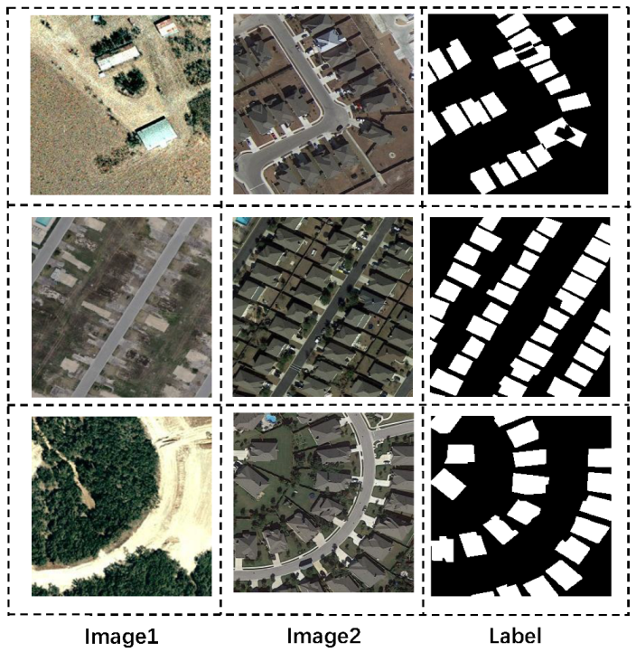
LEVIR-CD is a new large-scale building change detection dataset consisting of 637 pairs of ultra-high-resolution GE images with a size of 1024 × 1024. Its time span is 5–14 years, and it was taken from 2002 to 2018, focusing on significant changes in buildings. The bitemporal remote sensing images in the dataset are taken from 20 different areas in multiple cities in Texas, including villas, high-rise apartments, small garages, large warehouses, and other buildings. Seasonal and light changes are also taken into account to help develop effective algorithms. A schematic diagram is shown in Figure 8.

3.3. CDD

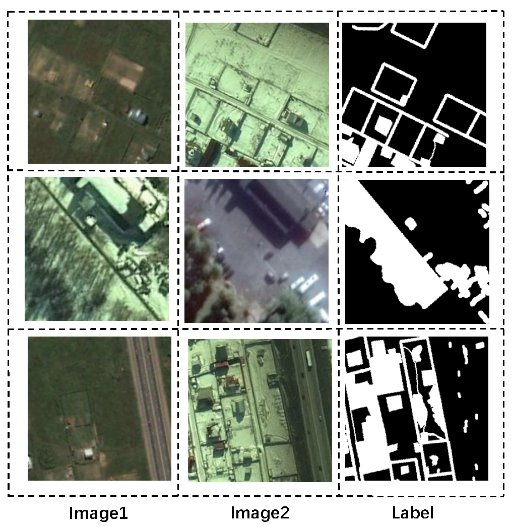
Compared with other CD datasets, most of the bitemporal images in the CDD dataset are taken in two different seasons from the same place, of which there are seven pairs of images with a size of 4725 × 2700 pixels. Due to the influence of seasonal illumination and other factors, the spectral feature information of the two images will be greatly different, which will lead to many false detections in the prediction. This can also further verify the ability of the model to process complex RS images. Figure 9 shows a sample diagram.

4. Experimental Comparison

Three sets of experiments are conducted to verify the performance of the proposed model. The pixel accuracy (PA), recall rate (RC), accuracy (PR), and joint average intersection (MIoU) are compared. PA represents the ratio of correct pixels. The proportion of the changed part is identified by RC in the original image, and PR represents the proportion of the correctly predicted pixel number in the changed area. MIoU represents the intersection and union ratio. Intersection is used to represent changing regions in CD tasks, and union represents invariant regions. Based on these four aspects, we can better verify the performance of the model.
P A = i = 0 k p i j i = 0 k j = 0 k p i j .
R C = T P T P + F N .
P R = T P T P + F P .
M I o U = 1 K + 1 i = 0 k p i i j = 0 k p i j + j = 0 k p j i p i i .

4.1. Parameter Setting

The learning rate must be reasonably set and selected. If the learning rate is too high, the loss rate of the model will be very severe, and the model will be difficult to converge. However, the learning rate cannot be set too low. If it is too low, it will increase the complexity of network convergence, which will also increase the difficulty of convergence, making the result the local minimum. Therefore, after comprehensive consideration, we adopt the random gradient descent method (SGD) to iterate the variable weight. Its learning rate l R is as follows:
l R = l r 1 i pr i max power ,
p o w e r is the initial momentum of 0.9, l r is the initial learning rate of 0.001, i m a x represents the maximum number of iterations, and i p r represents the number of current iterations.

4.2. Comparative Experiments of Different Backbone Networks

In the training process, on the premise that all parameters are set the same, we set up an experiment to study the performance difference between the backbone network the Multi-Scale Feature Extraction Network (MFEN) proposed in this paper and other backbone networks: DenseNet, ResNet, and GhostNet. As shown in Table 1, the MIoU indicators on the three datasets are 82.47%, 83.14%, and 73.85%. Compared with other existing feature extraction networks, it has a significant performance improvement. This is mainly because the MFEN that we designed passes the 3 × 3 convolution structure, and this is used to extract features of objects with different scales in the CD task. Compared with the traditional backbone feature extraction network, it significantly improves the ability to extract information.

4.3. Ablation Experiment and Its Thermodynamic Diagram

We performed ablation experiments on the three datasets. We verified the effectiveness of each submodule through the results of experiments involving different modules. In our experiments, we used a Multi-Scale Feature Extraction Network (MFEN) as a backbone network. The training parameter settings were the same. As shown in Table 2, the Feature Interaction Module (FIM) and the Detail Feature Guidance Module (DFGM) greatly improve the performance of the backbone network. This is because FIM makes the overall network pay more attention to local changes in terms of characteristics, and the edge feature information of the image is restored to the maximum extent by DFGM. Then, on this basis, multi-level features are fused through the MLP decoder (Decoder), which can more effectively remove some noise information so as to improve the accuracy of model prediction.
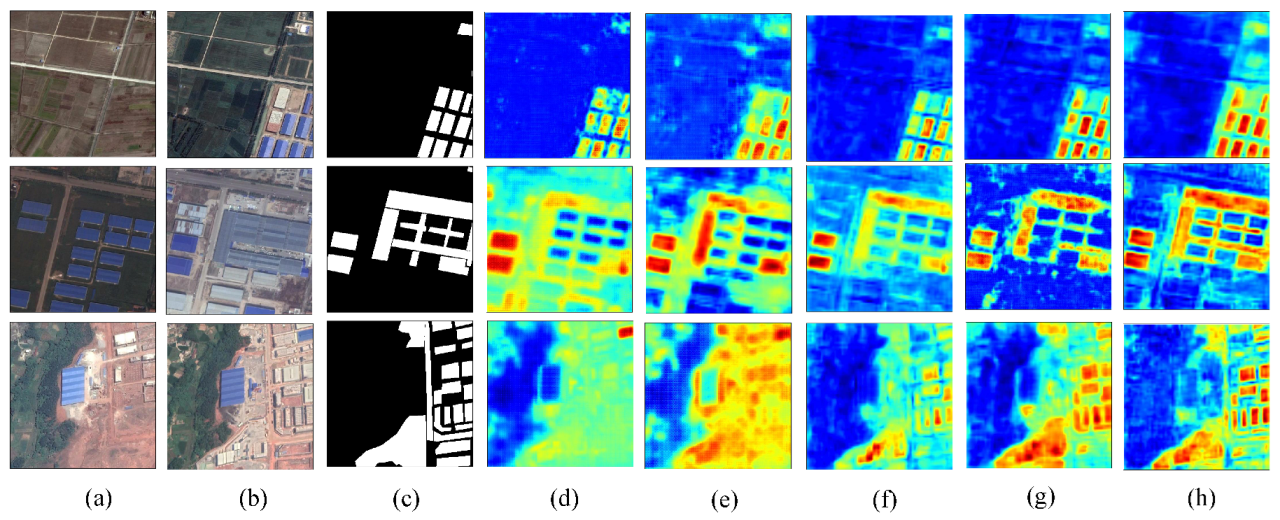
Figure 10 shows the heat maps of the ablation experiment, in which the red area represents the area that the model focuses on. In Figure 10, it can be seen that the model gives greater weights to the change area, because FIM fully considers the interaction of feature information between bitemporal RS images, which makes the model pay more attention to the change area. However, there are still many shortcomings in the edge details, so Figure 10g adds DFGM on this basis, from which it can be clearly seen that the prediction of edge details is greatly improved compared with the previous one. Finally, the feature information of different scales is fused and output by the MLP encoder, and the results are shown in Figure 10h. It can be seen that the model fully restores the edge detail information while paying attention to the change area, which also verifies the effectiveness of the MLP encoder proposed in this paper.

4.4. Comparison Experiment of Different Algorithms

In the comparison experiment, as the comparison algorithms, we choose the unsupervised algorithms IR-MAD and PCA-Means; the traditional semantic segmentation algorithms FCN, UNet, PSPNet, and BiseNet; and the CD algorithms FC-EF, STANet, SNUNet, and BIT. Furthermore, we carry out the experiment on three datasets. Section 3 describes the datasets used in the experiment. The experimental results are shown in Table 3. The accuracy of the unsupervised algorithm is far behind that of the supervised algorithm. Moreover, it is obvious that, compared with the CD algorithms, the experimental results of the traditional semantic segmentation algorithms are relatively poor, which is caused by their lack of design for the task characteristics of CD. In contrast, some existing CD algorithms perform better on these three datasets, but there are still some gaps between them and the algorithm in this paper. This is mainly because they do not take the feature interaction between a pair of input images into account when extracting the features of the bitemporal RS images, which makes the model not pay enough attention to the change area. The algorithm in this paper uses the Feature Interaction Module (FIM), designed to make the model pay more attention to important information with the deepening of network layers so as to reduce false detection and missed detection. Furthermore, through the Detail Feature Guidance Module (DFGM), the edge details of the image are restored to the maximum extent. Figure 11 shows a prediction diagram of three pairs of different algorithms selected from the test set. It is obvious that the traditional unsupervised algorithm can no longer handle the CD task under the complex background, and its prediction results are very rough. In contrast, the existing supervised algorithms can generally identify the change area, but the false detection and missed detection can be seen in Figure 11, showing especially rough edge details. The prediction results of the algorithm in this paper are shown in Figure 11. While correctly predicting the change area, the edge information in the image is also restored to the maximum extent so as to avoid the occurrence of false detection and missed detection to the maximum extent.

5. Conclusions

This paper proposes a Multi-Scale Feature Interaction Network (MFIN) model to detect changing regions in dual-temporal remote sensing (RS) images. Firstly, the multi-level feature information of the dual-temporal image is extracted through the Multi-Scale Feature Extraction Network (MFEN). Then, two submodules, the Feature Interaction Module (FIM) and the Detailed Feature Guidance Module (DFGM), are used to effectively interact with the feature information of the dual-temporal image, maximizing the restoration of image edge details. In the decoding section, a Multilayer Perceptron (MLP) encoder is designed as a decoder to fuse and decode multi-scale feature information. Finally, feature information of different scales is fused and upsampled for output. Moreover, a new RS-CD dataset is established. Furthermore, the advantages of the proposed algorithm are further verified through experiments. However, obtaining bitemporal RS datasets in practical tasks is relatively difficult, so in future research, semi-supervised or even unsupervised CD algorithms will be further studied.

Author Contributions

Conceptualization, C.Z. and Y.Z.; methodology, C.Z. and Y.Z.; software, C.Z.; validation, C.Z.; formal analysis, C.Z. and H.L.; investigation, C.Z. and H.L.; resources, Y.Z.; data curation, Y.Z.; writing—original draft preparation, C.Z.; writing—review and editing, H.L.; visualization, C.Z.; supervision, Y.Z.; project administration, Y.Z.; funding acquisition, Y.Z. All authors have read and agreed to the published version of the manuscript.

Funding

National Key Research and Development Program of China, grant number 2021YFE0116900.

Institutional Review Board Statement

Not applicable.

Informed Consent Statement

Not applicable.

Data Availability Statement

The data and the code of this study are available from the corresponding author upon request ([email protected]).

Acknowledgments

The authors would like to thank the Assistant Editor of this article and anonymous reviewers for their valuable suggestions and comments.

Conflicts of Interest

The authors declare no conflict of interest.

References

  1. Tison, C.; Nicolas, J.M.; Tupin, F.; Maître, H. A new statistical model for Markovian classification of urban areas in high-resolution SAR images. IEEE Trans. Geosci. Remote Sens. 2004, 42, 2046–2057. [Google Scholar] [CrossRef]
  2. Thompson, A.W.; Prokopy, L.S. Tracking urban sprawl: Using spatial data to inform farmland preservation policy. Land Use Policy 2009, 26, 194–202. [Google Scholar] [CrossRef]
  3. Sommer, S.; Hill, J.; Megier, J. The potential of remote sensing for monitoring rural land use changes and their effects on soil conditions. Agric. Ecosyst. Environ. 1998, 67, 197–209. [Google Scholar] [CrossRef]
  4. Fichera, C.R.; Modica, G.; Pollino, M. Land Cover classification and change-detection analysis using multi-temporal remote sensed imagery and landscape metrics. Eur. J. Remote Sens. 2012, 45, 1–18. [Google Scholar] [CrossRef]
  5. Gillespie, T.W.; Chu, J.; Frankenberg, E.; Thomas, D. Assessment and prediction of natural hazards from satellite imagery. Prog. Phys. Geogr. 2007, 31, 459–470. [Google Scholar] [CrossRef]
  6. Dong, L.; Shan, J. A comprehensive review of earthquake-induced building damage detection with remote sensing techniques. ISPRS J. Photogramm. Remote Sens. 2013, 84, 85–99. [Google Scholar] [CrossRef]
  7. Song, L.; Xia, M.; Weng, L.; Lin, H.; Qian, M.; Chen, B. Axial Cross Attention Meets CNN: Bibranch Fusion Network for Change Detection. IEEE J. Sel. Top. Appl. Earth Obs. Remote Sens. 2023, 16, 32–43. [Google Scholar] [CrossRef]
  8. Nielsen, A.A. The regularized iteratively reweighted MAD method for change detection in multi-and hyperspectral data. IEEE Trans. Image Process. 2007, 16, 463–478. [Google Scholar] [CrossRef]
  9. Abdi, H.; Williams, L.J. Principal component analysis. Wiley Interdiscip. Rev. Comput. Stat. 2010, 2, 433–459. [Google Scholar] [CrossRef]
  10. Chu, S.; Li, P.; Xia, M. MFGAN: Multi feature guided aggregation network for remote sensing image. Neural Comput. Appl. 2022, 34, 10157–10173. [Google Scholar] [CrossRef]
  11. Li, Q.; Zhong, R.; Du, X.; Du, Y. TransUNetCD: A Hybrid Transformer Network for Change Detection in Optical Remote-Sensing Images. IEEE Trans. Geosci. Remote Sens. 2022, 60, 5622519. [Google Scholar] [CrossRef]
  12. Zhang, Y.; Xu, W.; Yang, S.; Xu, Y.; Yu, X. Improved YOLOX detection algorithm for contraband in X-ray images. Appl. Opt. 2022, 61, 6297–6310. [Google Scholar] [CrossRef] [PubMed]
  13. Wang, Z.; Xia, M.; Lu, M.; Pan, L.; Liu, J. Parameter Identification in Power Transmission Systems Based on Graph Convolution Network. IEEE Trans. Power Deliv. 2022, 37, 3155–3163. [Google Scholar] [CrossRef]
  14. Qu, Y.; Xia, M.; Zhang, Y. Strip pooling channel spatial attention network for the segmentation of cloud and cloud shadow. Comput. Geosci. 2021, 157, 104940. [Google Scholar] [CrossRef]
  15. Gong, M.; Zhao, J.; Liu, J.; Miao, Q.; Jiao, L. Change detection in synthetic aperture radar images based on deep neural networks. IEEE Trans. Neural Netw. Learn. Syst. 2015, 27, 125–138. [Google Scholar] [CrossRef]
  16. Zhan, Y.; Fu, K.; Yan, M.; Sun, X.; Wang, H.; Qiu, X. Change detection based on deep siamese convolutional network for optical aerial images. IEEE Geosci. Remote Sens. Lett. 2017, 14, 1845–1849. [Google Scholar] [CrossRef]
  17. Varghese, A.; Gubbi, J.; Ramaswamy, A.; Balamuralidhar, P. ChangeNet: A deep learning architecture for visual change detection. In Proceedings of the European Conference on Computer Vision (ECCV) Workshops, Munich, Germany, 8–14 September 2018. [Google Scholar]
  18. Peng, D.; Bruzzone, L.; Zhang, Y.; Guan, H.; Ding, H.; Huang, X. SemiCDNet: A semisupervised convolutional neural network for change detection in high resolution remote-sensing images. IEEE Trans. Geosci. Remote Sens. 2020, 59, 5891–5906. [Google Scholar] [CrossRef]
  19. Parmar, N.; Vaswani, A.; Uszkoreit, J.; Kaiser, L.; Shazeer, N.; Ku, A.; Tran, D. Image transformer. In Proceedings of the International Conference on Machine Learning, Vienna, Austria, 25–31 July 2018; pp. 4055–4064. [Google Scholar]
  20. Wu, H.; Xiao, B.; Codella, N.; Liu, M.; Dai, X.; Yuan, L.; Zhang, L. Cvt: Introducing convolutions to vision transformers. In Proceedings of the IEEE/CVF International Conference on Computer Vision, Montreal, BC, Canada, 11–17 October 2021; pp. 22–31. [Google Scholar]
  21. Wang, W.; Xie, E.; Li, X.; Fan, D.P.; Song, K.; Liang, D.; Lu, T.; Luo, P.; Shao, L. Pyramid vision transformer: A versatile backbone for dense prediction without convolutions. In Proceedings of the IEEE/CVF International Conference on Computer Vision, Montreal, BC, Canada, 11–17 October 2021; pp. 568–578. [Google Scholar]
  22. Chen, H.; Qi, Z.; Shi, Z. Remote sensing image change detection with transformers. IEEE Trans. Geosci. Remote Sens. 2021, 60, 5607514. [Google Scholar] [CrossRef]
  23. Ma, Z.; Xia, M.; Weng, L.; Lin, H. Local Feature Search Network for Building and Water Segmentation of Remote Sensing Image. Sustainability 2023, 15, 3034. [Google Scholar] [CrossRef]
  24. Chen, B.; Xia, M.; Qian, M.; Huang, J. MANet: A multi-level aggregation network for semantic segmentation of high-resolution remote sensing images. Int. J. Remote Sens. 2022, 43, 5874–5894. [Google Scholar] [CrossRef]
  25. Miao, S.; Xia, M.; Qian, M.; Zhang, Y.; Liu, J.; Lin, H. Cloud/shadow segmentation based on multi-level feature enhanced network for remote sensing imagery. Int. J. Remote Sens. 2022, 43, 5940–5960. [Google Scholar] [CrossRef]
  26. Gao, J.; Weng, L.; Xia, M.; Lin, H. MLNet: Multichannel feature fusion lozenge network for land segmentation. J. Appl. Remote Sens. 2022, 16, 016513. [Google Scholar] [CrossRef]
  27. Lu, C.; Xia, M.; Lin, H. Multi-scale strip pooling feature aggregation network for cloud and cloud shadow segmentation. Neural Comput. Appl. 2022, 34, 6149–6162. [Google Scholar] [CrossRef]
  28. Wang, Q.; Wu, B.; Zhu, P.; Li, P.; Zuo, W.; Hu, Q. Supplementary material for ‘ECA-Net: Efficient channel attention for deep convolutional neural networks. In Proceedings of the 2020 IEEE/CVF Conference on Computer Vision and Pattern Recognition, Seattle, WA, USA, 14–19 June 2020; pp. 13–19. [Google Scholar]
  29. Chen, H.; Shi, Z. A spatial-temporal attention-based method and a new dataset for remote sensing image change detection. Remote Sens. 2020, 12, 1662. [Google Scholar] [CrossRef]
  30. Ji, S.; Wei, S.; Lu, M. Fully convolutional networks for multisource building extraction from an open aerial and satellite imagery data set. IEEE Trans. Geosci. Remote Sens. 2018, 57, 574–586. [Google Scholar] [CrossRef]
  31. Iandola, F.; Moskewicz, M.; Karayev, S.; Girshick, R.; Darrell, T.; Keutzer, K. Densenet: Implementing efficient convnet descriptor pyramids. arXiv 2014, arXiv:1404.1869. [Google Scholar]
  32. He, K.; Zhang, X.; Ren, S.; Sun, J. Deep residual learning for image recognition. In Proceedings of the IEEE Conference on Computer Vision and Pattern Recognition, Las Vegas, NV, USA, 27–30 June 2016; pp. 770–778. [Google Scholar]
  33. Han, K.; Wang, Y.; Tian, Q.; Guo, J.; Xu, C.; Xu, C. Ghostnet: More features from cheap operations. In Proceedings of the IEEE/CVF Conference on Computer Vision and Pattern Recognition, Seattle, WA, USA, 13–19 June 2020; pp. 1580–1589. [Google Scholar]
  34. Zhang, H.; Gong, M.; Zhang, P.; Su, L.; Shi, J. Feature-level change detection using deep representation and feature change analysis for multispectral imagery. IEEE Geosci. Remote Sens. Lett. 2016, 13, 1666–1670. [Google Scholar] [CrossRef]
  35. Long, J.; Shelhamer, E.; Darrell, T. Fully convolutional networks for semantic segmentation. In Proceedings of the IEEE Conference on Computer Vision and Pattern Recognition, Boston, MA, USA, 7–12 June 2015; pp. 3431–3440. [Google Scholar]
  36. Ronneberger, O.; Fischer, P.; Brox, T. U-net: Convolutional networks for biomedical image segmentation. In Proceedings of the International Conference on Medical image Computing and Computer-Assisted Intervention, Munich, Germany, 5–9 October 2015; Springer: Berlin/Heidelberg, Germany, 2015; pp. 234–241. [Google Scholar]
  37. Zhao, H.; Shi, J.; Qi, X.; Wang, X.; Jia, J. Pyramid scene parsing network. In Proceedings of the IEEE Conference on Computer Vision and Pattern Recognition, Honolulu, HI, USA, 21–26 July 2017; pp. 2881–2890. [Google Scholar]
  38. Yu, C.; Wang, J.; Peng, C.; Gao, C.; Yu, G.; Sang, N. Bisenet: Bilateral segmentation network for real-time semantic segmentation. In Proceedings of the European Conference on Computer Vision (ECCV), Munich, Germany, 8–14 September 2018; pp. 325–341. [Google Scholar]
  39. Daudt, R.C.; Le Saux, B.; Boulch, A. Fully convolutional siamese networks for change detection. In Proceedings of the 2018 25th IEEE International Conference on Image Processing (ICIP), Athens, Greece, 7–10 October 2018; IEEE: Piscataway, NJ, USA, 2018; pp. 4063–4067. [Google Scholar]
  40. Fang, S.; Li, K.; Shao, J.; Li, Z. SNUNet-CD: A densely connected Siamese network for change detection of VHR images. IEEE Geosci. Remote Sens. Lett. 2021, 19, 8007805. [Google Scholar] [CrossRef]
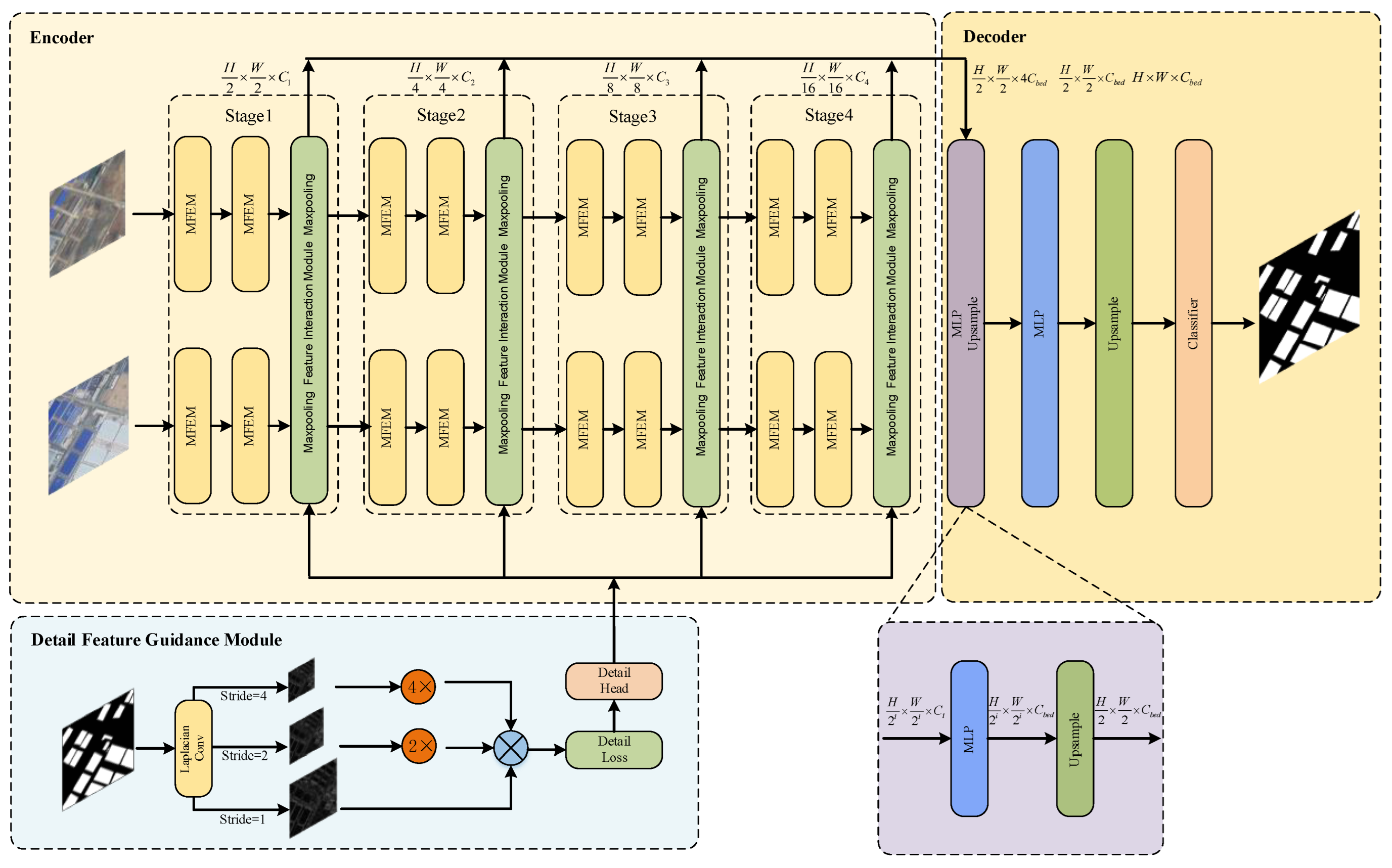
Figure 1. Structure diagram of Multi-Scale Feature Interaction Network (MFIN).
Remotesensing 15 02880 g001
Figure 2. Two groups of pictures (a,b) show that the pixel points cannot be well one-to-one corresponded due to illumination, season, and other factors.
Remotesensing 15 02880 g002
Figure 3. Structure diagram of the Multi-Scale Feature Extraction Network.
Remotesensing 15 02880 g003
Figure 4. Structure diagram of the Feature Interaction Module.
Remotesensing 15 02880 g004
Figure 5. Comparison of heat maps of FIM. (a,b) Bitemporal RS images. (c) The labels. (d) The basic network without FIM’s heat maps. (e) The basic network with FIM’s heat maps.
Remotesensing 15 02880 g005
Figure 6. Sample example diagrams in BRSCDD.
Remotesensing 15 02880 g006
Figure 7. Statistical analysis of datasets.
Remotesensing 15 02880 g007
Figure 8. Partial sample diagrams of LEVIR-CD.
Remotesensing 15 02880 g008
Figure 9. CDD sample.
Remotesensing 15 02880 g009
Figure 10. Ablation experiment and its thermodynamic diagram: (a,b) a pair of RS images, (c) its label, (d) MFEN, (e) MFEN + FIM, (f) MFEN + DFGM, (g) MFEN + FIM + DFGM, (h) MFEN + FIM + DFGM + Decoder.
Remotesensing 15 02880 g010
Figure 11. Comparison diagrams of experiment on three public dataset, where (ac) are from BRSCDD; (df) are from LEVIR-CD; (gi) are from CDD.
Remotesensing 15 02880 g011
Table 1. Comparison of performance of different backbone networks (the best results are in bold).
BackboneBRSCDDLEVIR-CDCDD
MIoU (%)MIoU (%)MIoU (%)
DenseNet121 [31]81.1081.0672.29
DenseNet161 [31]81.6581.4272.53
ResNet-18 [32]81.3082.2972.77
ResNet-34 [32]81.7382.8772.94
GhostNet [33]81.2782.6272.83
MFEN82.4783.1473.85
Table 2. Comparison of ablation experimental data (the best results are in bold).
BakeboneFIMDFGMDecoderBRSCDDLEVIR-CDCDD
MIoUMIoUMIoU
MFEN77.3778.8769.44
80.3781.9371.69
79.9581.2871.27
81.5982.5672.70
82.4783.1473.85
Table 3. Comparison of final experimental data (best results are in bold).
MethodBRSCDDLEVIR-CDCDD
PA/RC/PR/MIoUPA /RC/PR/MIoUPA/RC/PR/MIoU
IR-MAD [8]33.52/45.15/17.20/42.9327.52/41.35/13.58/31.2423.91/35.82/12.79/25.63
PCA-Means [34]38.93/49.33/21.82/48.5731.24/46.29/17.81/37.1229.31/38.54/15.87/29.75
FCN [35]92.13/63.92/73.42/74.8195.13/67.92/69.42/76.8194.46/44.97/53.58/61.96
UNet [36]93.26/64.04/75.49/76.0496.77/70.25/71.15/78.9794.03/45.81/56.79/62.58
PSPNet [37]93.87/66.85/75.86/77.5595.89/69.73/72.71/77.1595.15/48.26/58.98/67.43
BiseNet [38]94.19/66.39/74.82/77.7995.03/67.17/68.79/74.8296.03/52.19/61.40/69.58
FC-EF [39]94.13/66.74/73.69/77.5195.25/68.72/70.35/76.8695.58/50.82/61.51/68.73
STANet [29]94.72/66.52/78.68/79.1595.37/70.14/71.05/78.2796.02/53.41/62.54/71.07
SNUNet [40]94.73/68.39/78.85/80.2397.03/70.71/72.25/80.4796.18/56.03/64.28/73.09
BIT [22]95.27/69.89/79.44/81.3397.35/71.62/72.54/81.0696.03/55.95/63.41/72.53
MFIN(ours)97.73/71.32/80.87/82.4797.07/71.02/72.98/83.1496.84/56.24/65.19/73.85
Disclaimer/Publisher’s Note: The statements, opinions and data contained in all publications are solely those of the individual author(s) and contributor(s) and not of MDPI and/or the editor(s). MDPI and/or the editor(s) disclaim responsibility for any injury to people or property resulting from any ideas, methods, instructions or products referred to in the content.