Article

A Novel Deep Stack-Based Ensemble Learning Approach for Fault Detection and Classification in Photovoltaic Arrays

1
The SKL for Management and Control of Complex Systems, Institute of Automation, Chinese Academy of Sciences, Beijing 100190, China
2
The School of Artificial Intelligence, University of Chinese Academy of Sciences, Beijing 100049, China
3
The Beijing Engineering Research Center of Intelligent Systems and Technology, Institute of Automation, Academy of Sciences, Beijing 100190, China
4
School of Mechanical and Precision Instrument Engineering, Xi’an University of Technology, Xi’an 710048, China
5
Department of Mechatronics Engineering, University of Chakwal, Chakwal 48800, Pakistan
6
Department of Computer and Technology, Chang’an University, Xi’an 710062, China
*
Author to whom correspondence should be addressed.
Remote Sens. 2023, 15(5), 1277; https://doi.org/10.3390/rs15051277
Submission received: 12 January 2023 / Revised: 19 February 2023 / Accepted: 23 February 2023 / Published: 25 February 2023
(This article belongs to the Special Issue Remote Sensing for Green Energy Development)

Abstract

:
The widespread adoption of green energy resources worldwide, such as photovoltaic (PV) systems to generate green and renewable power, has prompted safety and reliability concerns. One of these concerns is fault diagnostics, which is needed to manage the reliability and output of PV systems. Severe PV faults make detecting faults challenging because of drastic weather circumstances. This research article presents a novel deep stack-based ensemble learning (DSEL) approach for diagnosing PV array faults. The DSEL approach compromises three deep-learning models, namely, deep neural network, long short-term memory, and Bi-directional long short-term memory, as base learners for diagnosing PV faults. To better analyze PV arrays, we use multinomial logistic regression as a meta-learner to combine the predictions of base learners. This study considers open circuits, short circuits, partial shading, bridge, degradation faults, and incorporation of the MPPT algorithm. The DSEL algorithm offers reliable, precise, and accurate PV-fault diagnostics for noiseless and noisy data. The proposed DSEL approach is quantitatively examined and compared to eight prior machine-learning and deep-learning-based PV-fault classification methodologies by using a simulated dataset. The findings show that the proposed approach outperforms other techniques, achieving 98.62% accuracy for fault detection with noiseless data and 94.87% accuracy with noisy data. The study revealed that the DSEL algorithm retains a strong generalization potential for detecting PV faults while enhancing prediction accuracy. Hence, the proposed DSEL algorithm detects and categorizes PV array faults more efficiently, reliably, and accurately.

1. Introduction

The need for renewable energy sources has grown in recent years due to environmental concerns and the scarcity of conventional energy sources. This universe has enormous green energy potential. Recently, solar, wind, tidal, and geothermal energy have become increasingly well-known as reliable, stable, and significant energy sources. Solar power is among the most effective green energy sources [1,2,3]. Due to its abundance, durability, and sustainability, solar energy is undoubtedly a vital renewable energy source. The power generated by a PV panel is proportional to the total amount of solar radiation received on its surface; this solar radiation comes either directly from the sun or indirectly through diffusion or reflection. PV systems are popular because of their accessibility, adaptability, flexibility, eco-friendliness, availability, simple design, minimal air pollution, and fuel cost [4,5]. For instance, PV power generation would minimize carbon dioxide discharges by around 69 to 100 million tons by 2030 [6]. The installed capacity of the solar industry around the world has gradually expanded since 2011; between 2017 and 2022, solar power installations were expected to add up to 438 GW, according to the Inter-National Renewable Energy Agency (IRENA). Solar farms or rooftop PV-generating stations could provide electricity and manage various loads [7,8]. Despite having many positive qualities, the PV system faces significant challenges, such as reliability issues, low power output, high initial investment requirements, dependence on environmental conditions, such as temperature and humidity, and vulnerability to faults. Fault susceptibility in PV systems is one of many critical issues that must be solved.
This paper addresses the severe and challenging issue of detecting and classifying PV system faults. The photovoltaic (PV) array is a fundamental component of PV systems that generate electricity for the grid and is typically installed outdoors in harsh, challenging, and severe environmental conditions. With the proliferation of power electronic devices and non-linear loads, the power quality of the distribution grid has deteriorated, as reported by Kerrouche et al. [9]. Furthermore, Lodhi E. et al. investigated that thunderstorms, shadows, and physical or temperature impacts on wire insulation can induce faults in PV arrays. These incidents can substantially decrease the PV system’s efficacy and output power [10]. For example, [11] presented a PV system monitoring study in which a loss of annual energy of 18.9 percent has been reported due to multiple faults. Faulty PV arrays can lead to fires or explosions, putting lives and property at risk. As an illustration, ground fault created a fire hazard in Bakersfield, California, as documented by the authors. In addition, the authors stated that a big PV plant in the state of California in the United States was involved in a fire hazard due to a short-circuit fault [12,13]. The PV array is susceptible to experiencing various faults (including open circuits, short circuit, ground, line-to-line, arc, hot spot, bridge, partial shading, and degradation faults) [14]. PV faults are potentially dangerous events that require immediate attention and response. Early detection of these issues is extremely important to warn the user of impending PV system failures. This has encouraged researchers to focus more on overcoming PV system interference, such as fault detection and diagnostics. Various fault classification and diagnosis techniques have been developed to address the challenges mentioned above for protecting PV systems. These PV-fault-diagnostic techniques can be classified into four categories: protective devices, signal processing-based models, performance comparison-based models, and artificial intelligence-based models.
The first category makes faults diagnostic by utilizing protective devices. The national electrical installation code suggests using an overcurrent protection device, an arc fault circuit interrupter, and a ground fault protection device to identify line-to-line, arc, and line-to-ground faults, respectively [15,16]. These safety devices have fuses that melt when the fault current exceeds their rating, isolating the fault. On the other hand, these protective devices cannot detect PV array faults with lower fault current magnitudes. Hence, faults may be undiscovered for an extended period, demonstrating the limitations of conventional PV array protection mechanisms. The second domain utilizes signal processing-based models (the working principle is reflected signals) to detect PV array faults. Time domain reflectometry (TDR) diagnoses and locates faults using the time-specific features of reflected signals. TDR introduces a signal of external voltage into the system and examines the impedance variation in the rejected signal. In [17], a 1 MW PV system was analyzed experimentally, utilizing TDR to identify faults in PV arrays. The spread spectrum time domain reflectometry is mentioned in another study [18] to locate and detect line-to-ground faults. However, its accuracy is substantially affected by the device’s distance from the fault spot. However, these methods could be more cost-effective since they need supplementary equipment and development tools to extract the signals’ features. The third domain employs performance comparison-based techniques to detect PV array faults. There are two primary approaches used in performance comparison-based techniques. In the first approach, threshold limits are compared to real-time parameters. The second approach evaluates the experimental constraints by comparing them to the predicted values of the PV model’s constraints. In [19], a fault detection approach is presented to compute the power loss by correlating monitored and expected AC output power. The research [20] reported an entropy-based technique to detect open circuit, line-to-line faults even when blocking diodes are present. A study [21] conducted a fault detection technique that estimated the projected maximum power using the MPPT algorithm and compared it to the power measured by the meter. In [22], Hariharan et al. presented a fault-diagnosis methodology to differentiate line-to-line faults from normal and shading fault conditions. However, the suggested method is inapplicable to larger PV farms with different solar irradiances on PV modules. The precision of the aforementioned techniques is proportional to the value of the threshold limit. Despite its simplicity and the model’s dependence on MPPT operation, MPPT failure may affect the diagnosis efficiency of these performance measurement techniques. In addition, the model must be periodically updated because PV parameters are extremely reliant on weather changes.
For detecting and classifying PV faults, the fourth domain employs artificial intelligence-based algorithms. In [23], a fault detection approach is proposed based on an SVM classifier to identify short-circuit faults. However, multiple filters are needed, which makes this method costly. Chen et al. [24] developed an optimized kernel extreme learning machine (KELM) technique to diagnose an open circuit, short-circuit partial shading, and degrading faults. This approach has a high-performance ratio for experimental and simulated scenarios, but its computational time is high compared to other techniques. A graph-based semi-supervised learning technique is reported in [25] to identify and classify PV. The ANN method has been implemented in a monitoring system for PV panels to forecast the output power for detecting degradation [26]. When data is noisy, the ANN model cannot be used. Deep learning has recently attracted considerable attention due to its capability to accommodate complex datasets and advancements in computing capacity. A variety of ANN designs, from a basic and simple ANN network to more complex and complicated models, such as auto-encoder [27], self-organizing maps [28], and LSTM [29] networks, have been effectively used to forecast the production of PV power plants. A probabilistic neural network (PNN) algorithm in [30] examines the PV array in the presence of blocking diodes to evaluate the influence of line-to-line and line-to-ground faults. However, the proposed method does not consider faults with a high impedance. Its relevance to real PV arrays has yet to be verified, and its implementation is complicated and expensive. Multiple layers of perceptron neural networks have been created and successfully identify PV faults [31]. However, this study needs great consideration because extracting features from a wavelet and finding the hidden layer in a neural network architecture is hard. The authors [32] designed a deep residual network for detecting PV faults. The model exhibits good classification accuracy in simulated and experimental conditions. However, this model only detected line-to-line and open circuit faults. An AdaBoost ensemble approach is proposed to diagnose PV array faults [33]. It showed good detection accuracy of about 97.58%, but it only detected open circuits, short circuits, and degradation faults. Another complicated approach is discussed using CNN, AlexNet, and SVM [34]. However, the results showed relatively low accuracy, between 69.39 and 73.53 percent. A supervised learning technique follows the multilayer perceptron for fault detection in PV systems [35]. However, this technique is constrained to particular environmental conditions, as the study only collects data during winter. A literature review revealed that fault detection is challenging due to degradation, high impedance, MPPT, and power supply. Therefore, previous studies conclude that more research is still needed for more robust performance.
Ensemble learning methods have recently seen widespread application across many fields of study. Ensemble learning-based methodologies have been implemented for anomaly detection, fault diagnostics, and PV energy estimation [36,37]. An ensemble learning-based approach is introduced for the next day’s PV output power prediction in smart grids [38]. This model illustrates that the proposed framework outperforms individual and benchmark models in terms of accuracy. However, this model has limitations when dealing with time series data. The ensemble learning approach is suggested for diagnosing line-to-line faults by combining naive Bayes, SVM, and KNN classifiers. These classifiers performed well under various conditions [39]. Another research [40] investigated bagging and stacking-based ensemble learning for anomaly detection in the energy production of grid-interfaced PV systems. The results obtained 94 percent for stack-based ensemble learning and 79.50 percent for bagging-based ensemble learning. Wu et al. [41] presented a radial basis function (RBF) kernel extreme learning machine (ELM) using a simulated annealing (SA) approach for the identification of partial shading, short circuit, and aging defects in the PV system. The proposed model boosts accuracy, but training and testing times are longer than ELM or RBF-ELM. Consequently, the suggested methodology is slower. Another study utilized the ensemble learning model compromising decision tree, quadratic discriminant analysis, and extra trees with entropy [42]. This model detected partial shading and short-circuit faults with 97.46% accuracy before and 97.67% after optimization. Overall, these fault identification algorithms have produced promising diagnostic outcomes. Most of these methods, however, depend on manually extracting features, which requires an expert level of familiarity with signal processing and diagnostics. Furthermore, manual feature extraction is time-intensive and costly because of many filter requirements. Hence, better performance is still needed for an ensemble learning-based method that accurately diagnoses various faults in PV arrays.
This research article presents a novel deep stack-based ensemble learning (DSEL) algorithm for diagnosing and evaluating PV system faults that overcome the limitations of previous research. The DSEL approach integrates deep neural network (DNN), long short-term memory (LSTM), and Bi-directional long short-term memory (Bi-LSTM), three distinct deep-learning models, as base learners for diagnosing PV faults. Multinomial logistic regression (MLR) as a meta-learner is used to integrate the predictions from the base learners. With optimal parameters for weak or base learners, the results demonstrate that the suggested approach enhances the classification performance and retains a powerful generalization capability for PV system fault diagnosis. The proposed DSEL approach provides reliable and accurate PV-fault diagnostics for noiseless and noisy data. The comprehensive and deep quantitative assessment of the suggested DSEL algorithm is compared to eight earlier classification approaches (both classical machine-learning and deep learning-based), such as Probabilistic neural network, Bi-LSTM, LSTM, DNN, ANN, Gradient Boost, Support vector machine, AdaBoost, and Random forest. For a meaningful comparison, all these fault-diagnosis techniques will be statistically evaluated on a consistent dataset. This consistent comparison examination has not been explored in the previous fault-diagnosis literature. Instead, the authors selected to apply their methodologies to datasets collected under various environmental circumstances and system configurations, with varying array sizes and characteristics, often only two or three fault categories, and usually without MPPT. Therefore, comparing the performance provided in one research work to that presented in another is almost meaningless in past research on fault diagnosis. Furthermore, in contrast to recent studies, this research considers five distinct faulty conditions and one no-fault condition: open circuit fault, short-circuit fault, bridge fault, partial shading fault, degradation fault condition, and no-fault condition. Very little work has been performed on these specific faults in the deep-learning domain. Furthermore, this research article uses the DSEL approach for the first time to analyze, classify, and detect these specific PV array faults. Future studies on fault diagnosis for PV array systems will benefit from this research work. The significant contributions of the proposed research work are mentioned as follows:
  • Designing a novel deep stack-based ensemble learning (DSEL) approach for PV-fault diagnosis with deep base learners based on a probabilistic strategy without intensive hyperparameter tuning;
  • A thorough review of fault-diagnosis techniques published in earlier studies has been conducted to better comprehend the effectiveness and performance of the proposed DSEL approach compared to other methods;
  • The key features have been collected by examining the fluctuations in the I–V characteristic curves of PV arrays under normal and fault conditions;
  • The proposed DSEL methodology can identify and categorize defects through many critical scenarios with high impedances, low mismatch, irradiance levels, etc.
The rest of this paper is organized as follows: Section 2 presents the description of the PV system and related faults, while Section 3 provides the framework for the proposed DSEL fault-diagnosis algorithm. Then, simulation results evaluation and comparison with other techniques are analyzed in Section 4. At last, the conclusion and future directions of this study are presented in Section 5.

2. Description of PV System and Related Faults

PV systems are frequently divided into grid-interfaced and stand-alone systems based on their possible applications. The schematic diagram of the grid-interfaced PV system under consideration is depicted in Figure 1. In addition to PV modules, a grid-interfaced PV system comprises PV arrays, a DC-to-DC boost converter, an MPPT tracker, DC-to-AC three-phase inverter, protective devices, and auxiliaries. The PV array under investigation comprises five parallel strings, each with five series modules. The maximum power point tracking (MPPT) technique controls the boost converter’s switching, which monitors the duty cycle. This research uses the dragonfly optimization (DFO) algorithm to regulate and control the DC-to-DC converter’s duty cycle, as reported in [43]. In order to integrate with the grid, DC power from PV modules must be converted to AC power using an inverter.

2.1. Modelling of the PV Array

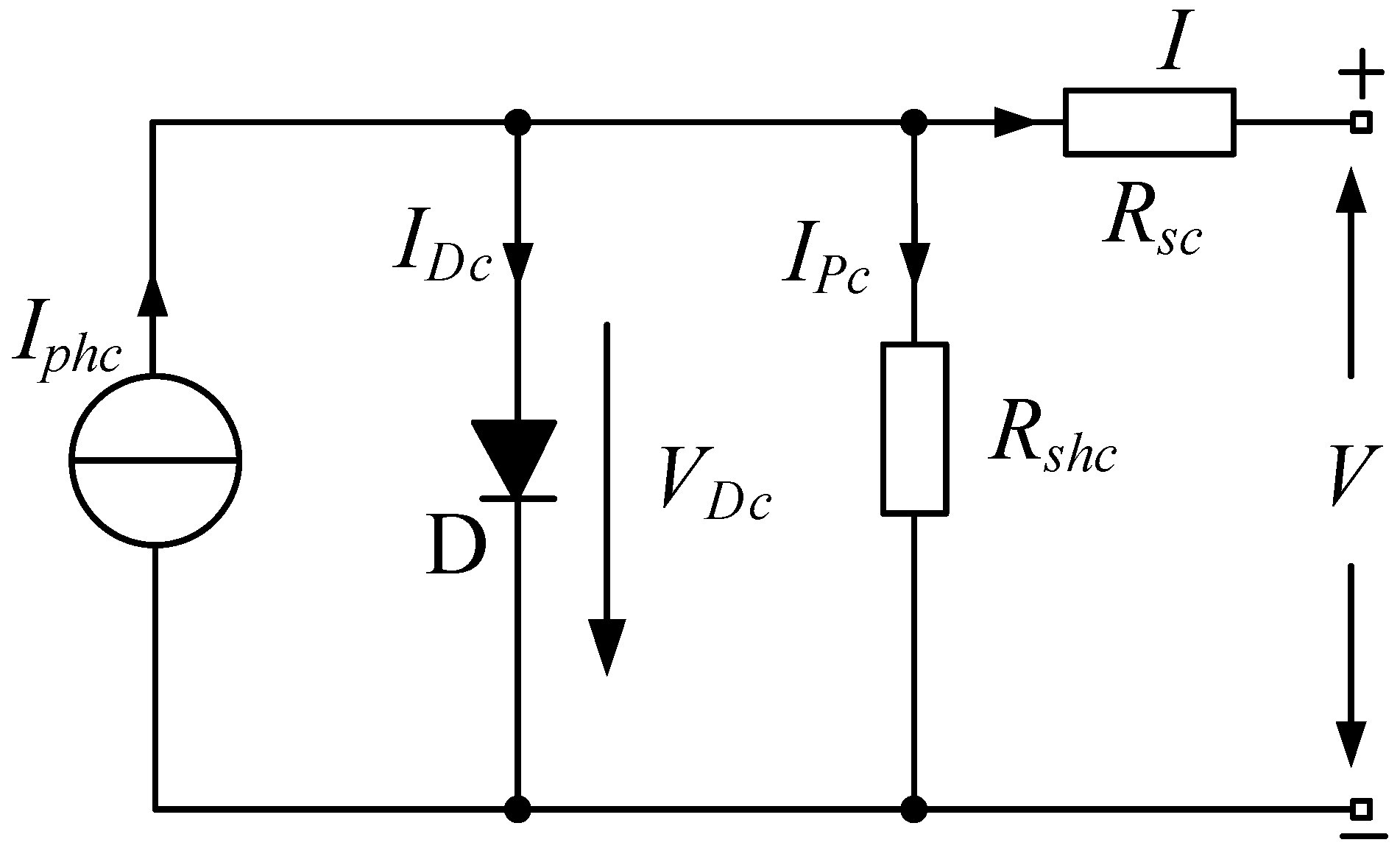
PV cells are often characterized using either a single or double-diode model. The superiority of two-diode models has been established. However, its popularity is limited by further parameter limits. The single-diode form is preferred due to its lower cost and advantageous balance of precision and convenience. As a result, the one-diode model is adopted in this study, as it has been in previous pioneer studies [10]. Figure 2 displays the equivalent one-diode PV module model.
I = I p h c I 0 { exp ( q ( V + I × R s c ) n k T ) U + I × R s c R s h c }
where I p h c and I 0 are the photogenerated current and reverse saturation current of the PV module, respectively, T is the operating temperature, and K is the Boltzmann constant, q is the electron charge, and V is the module’s output voltage. The analogous series resistance is denoted by R s c , and the corresponding parallel resistance is denoted by R s h c . The specifications for the BP-MSX 120 Module’s output characteristics under standard test conditions (STC) are listed in Table 1. Numerous PV cells are coupled in series to make a PV module, and PV modules are successively linked in series and parallel to make a PV string. The collection of these PV strings is called a PV array. The PV array is a collection of PV strings. These PV arrays can produce electricity in response to the intended demand. Assume that N p c and N s c are the numbers of cells in parallel and series, respectively. As a result, Equation (1) can be transformed into Equation (2).
I = ( I p h c . N p c ) ( I 0 . N s c ) × { exp ( q ( N p c N s c × I × R s c + V ) n k T N s c ) 1 }
Table 1. The specifications for the BP-MSX 120 PV module at STC [34].
ParameterValues
Short-Circuit Current3.87 (A)
Maximum Current3.56 (A)
Open Circuit Voltage42.1 (V)
Maximum Voltage33.7 (V)
Maximum Power120 (W)
Maximum Series Fuse Rating10a
Operating Temperature(−40~+85) °C
Figure 2. A PV module’s equivalent circuit diagram.
Remotesensing 15 01277 g002

2.2. Fault Analysis in PV System

PV systems can occasionally experience a variety of electrical faults because of many internal layout abnormalities [14]. The PV array under investigation comprises five parallel strings, each with five series modules. In contrast to recent studies, this research considers five distinct faulty conditions and one no-fault condition. Figure 1 displays the faults examined for the research to undertake a qualitative assessment of the proposed DSEL algorithm and its comparison with other traditional ML and DL-based fault-diagnostic techniques. A detailed discussion regarding these specific faults is described below.

2.2.1. Open Circuit Fault

An incidental disconnection issue within a string or between two neighboring strings is known as an open circuit fault in PV arrays [15]. It can happen for various causes, including a broken cable connecting two strings, something dropping on solar panels, or a loose connection between two points. The open voltage in these circumstances remains virtually constant, while the maximum power and short current drop drastically as the quantity of disconnected strings increases.

2.2.2. Short-Circuit Fault

A sudden short circuit between two PV array locations at various potential levels causes short-circuit faults. It might happen within the same string or across two adjacent strings [12], causing a fire disaster. The magnitude of a short-circuit fault is often determined by mismatch level and fault path impedance. When a short-circuit defect occurs, the PV arrays’ open-circuit voltage rapidly drops, whereas the short-circuit current remains constant as in any other regular string.

2.2.3. Bridge Fault

The bridge fault refers to a low-resistance link between two potential places in a string of modules or wires. The bridge fault typically results in lower array voltage but only a slight change in array current. The bridge fault typically results in a lower array voltage but only a little drop in array current. A higher voltage difference between the fault sites reduces open circuit voltage, maximum current, and maximum voltage, respectively.

2.2.4. Partial Shading Fault

This is known as a partial shading fault condition when certain modules are completely shaded and others are partially shaded. It is a transient situation that results in a temporary drop in power [43]. There can be two categories of shading. The first is static shading, and the second is dynamic shading. Static shading is created by exposure to leaves, dust, and bird droppings on solar panels. In contrast, dynamic shading is caused by the temporary shadow cast by surrounding trees, buildings, or overhead power lines. The shaded part in dynamic shading changes throughout time, resulting in a continual variation in output power. The occurrence of several peaks in PV characteristics is caused by partial shading. During PSF, there is a tremendous decrease in short-circuit current; however, open-circuit voltage gradually reduces.

2.2.5. Degradation Fault

The degradation fault occurs due to increases in the value of series resistance between the PV modules because of corrosion caused by water vapors or poor adherence of contacts. The consequence of this fault is a reduction in the array’s power output because of the increase in the resistance value. However, this fault scenario has noticed no change in open circuit voltage and short-circuit current. Raising internal series resistance might lead to a reduction in peak power.
PV systems are commonly affected by several electrical defects induced by several irregularities in the configuration of PV arrays [14]. As seen in Figure 3a, when a fault happens among PV panels, the power output from the array varies widely, even though the operational characteristics of a single PV panel do not differ substantially. Figure 3a shows the power-voltage characteristic curves under the normal and faulty scenarios, while Figure 3b shows the current-voltage characteristic curves under the normal and faulty scenarios. The short-circuit current will drop significantly if a PV array experiences an open circuit fault. When a short-circuit fault occurs, the open-circuit voltage declines significantly. The consequences of bridge fault are a reduction in open circuit voltage and a smaller decrease in the short-circuit current of PV arrays. The P-V and I-V operating curves behave differently under partial shading fault conditions. The open circuit voltage gradually reduces; however, a tremendous decrease is observed in the short-circuit current experience during partial shading fault. Compared to the typical PV array operation, the degrading fault causes a reduction in the maximum current and voltage; however, no changes have been observed in the PV array’s open-circuit voltage or short-circuit current.

3. Proposed Fault-Diagnosis Model

There are two important phases when attempting to diagnose a fault with PV arrays—the first phase in PV-fault diagnostics is collecting and processing raw data, and the second is using a proposed algorithm to recognize and classify faults in PV systems. Figure 4 depicts a workflow diagram for the proposed DSEL fault-diagnosis technique. The steps of this workflow research investigation are examined and analyzed in detail in the following sections.

3.1. Data Acquisition and Preprocessing

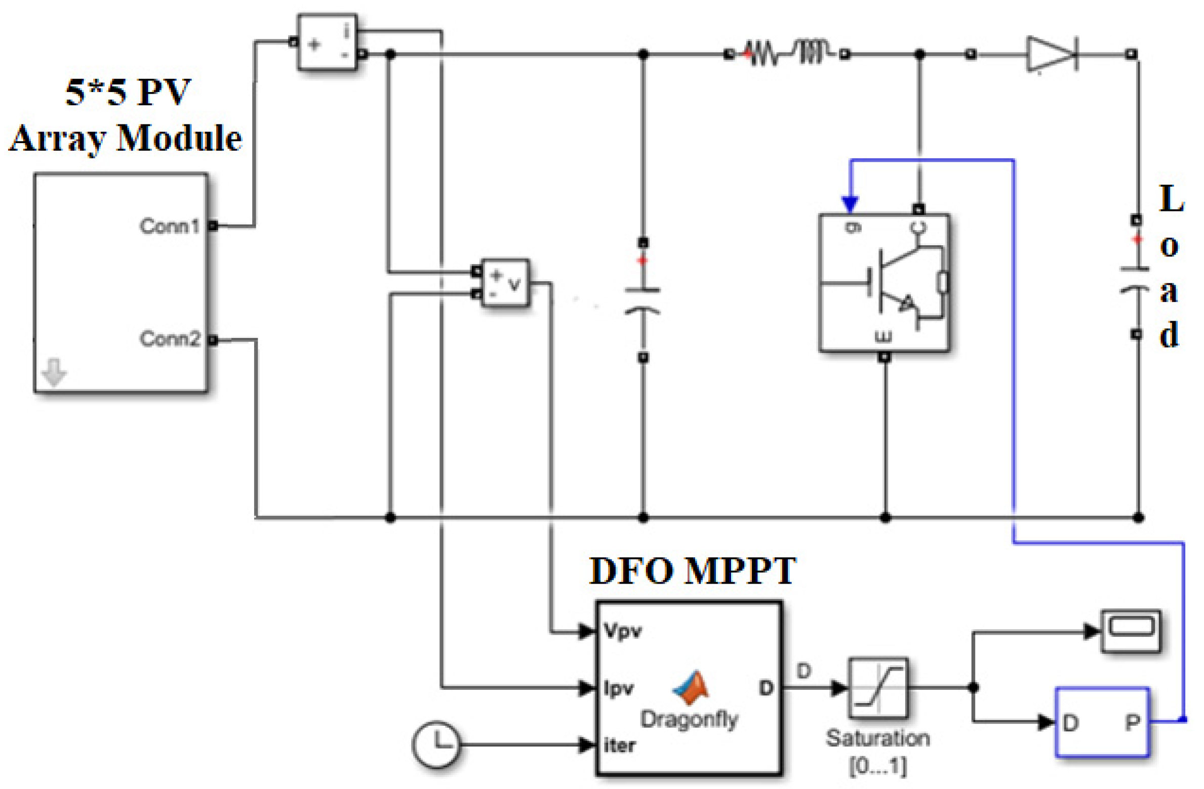
Deep-learning algorithms work effectively when sufficiently trained on massive amounts of data. Unfortunately, gathering extensive field data (made up of faulty and standard samples) for any given PV array-operating scenario is impractical. The PV array’s unpredictable ambient temperature and solar irradiation cause this impracticability. In addition, presenting an accurate PV system set up to the faults reported in this study can result in substantial damage and hazardous circumstances. Because of this, simulation is used to obtain the data used in this research. The model of the PV system utilized to acquire the data is presented in detail here, along with a description of faulty cases and the data itself. To examine the efficacy of the proposed DSEL methodology, a dataset is gathered in both faulty and non-faulty operational circumstances using the MATLAB Simulink model for a PV system, as shown in Figure 5. Six cases are taken into account when analyzing the suggested DSEL algorithm, including open circuit (OC-Fault), short circuit (SC-Fault), bridge (B-Fault), partial shading (PS-Fault), degradation (D-Fault), and no-fault (No-Fault) conditions, as shown in Figure 1 of Section 2. Nine parameters extracted for the data attributes are irradiance, temperature, open circuit voltage, short-circuit current, form factor, maximum current, maximum voltage, maximum power, and output power from the boost converter. Since these nine parameters are affected by PV system faults directly or indirectly, they serve as representative datasets. In total, 3636 data samples and labels were gathered. There are 606 instances of each class (No-Fault, SC-Fault, OC- Fault, PS-Fault, B-Fault, and D-Fault). These 3636 samples were generated by executing PV array simulations for the six scenarios indicated in Table 2 with different combinations of parameter values adopted for data collection.
In addition, the proposed DSEL algorithm is made to be compared with other PV-fault-diagnosis techniques and will be statistically evaluated on this consistent dataset, as observed in Table 2. This consistent dataset comparison investigation has not been conducted in the earlier fault-diagnostic literature. Data missing and standardization are problems arising during processing and extracting PV array characteristic parameters. A lack of information for some variables is known as missing data. There are several potential sources of data missing, such as equipment failures, human error in data entry, and others. The average filling technique is utilized to approximate the missing values. In addition, data standardization is essential to enhance the dataset’s overall reliability by transforming and standardizing.

3.2. Ensemble Learning-Based Algorithms

3.2.1. Ensemble Learning (EL)

The ensemble learning (EL) technique combines several base learner algorithm pattern schemes when creating an ideal prediction model. The developed ideal prediction model performs much better than the base learner algorithms alone. From this perspective, this section attempts to demonstrate the critical aspects and concepts of those techniques necessary to understand this study.

3.2.2. Stacking

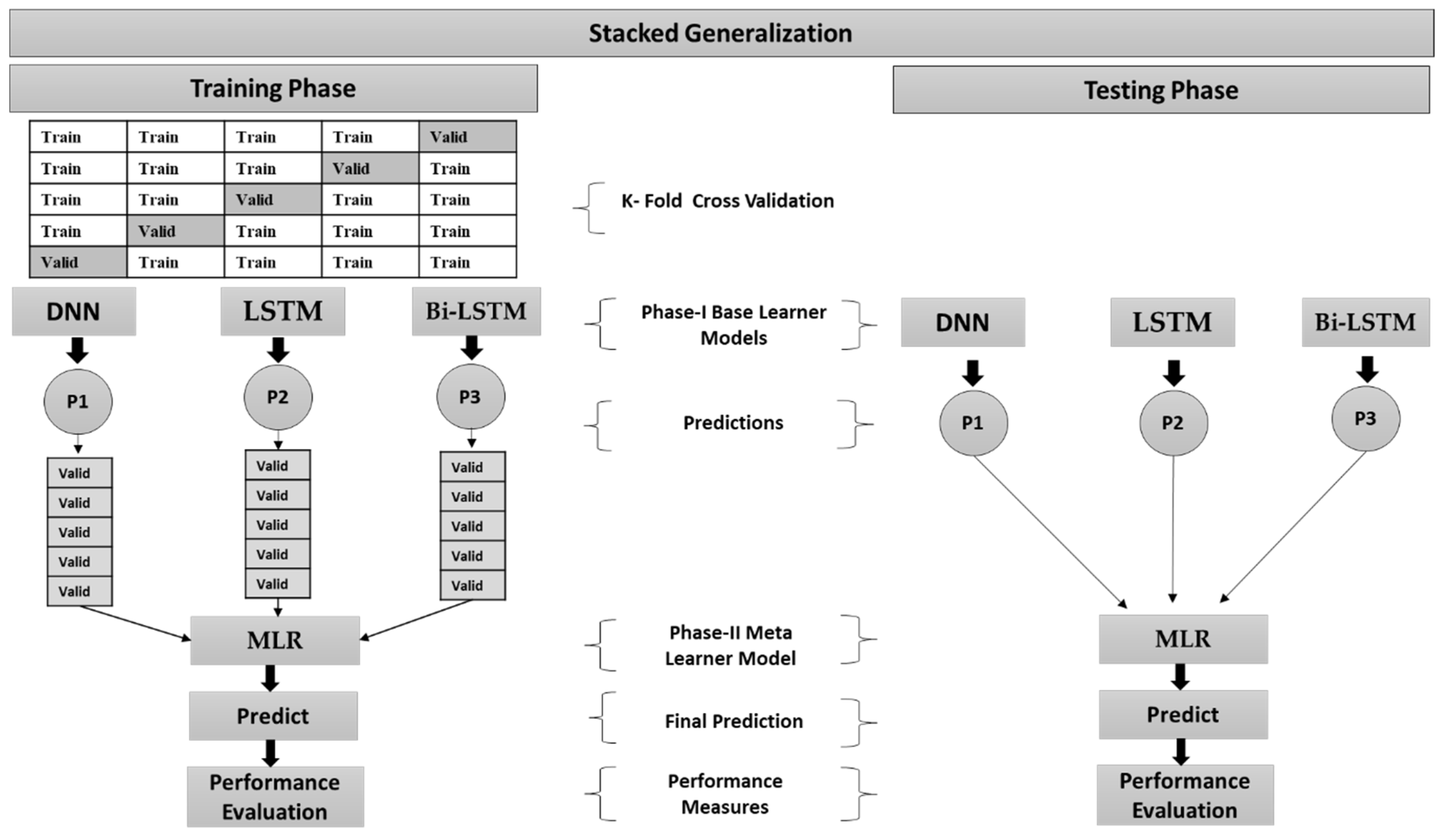
Another ensemble learning (EL) method developed by Wolpert is stacking or stacked generalization, which has been extensively applied in numerous domains since its inception [40]. Stacking combines the outcomes of multiple base learner models required to train a new meta-learner model for the output result. The fundamental idea of stacking is built on two stages of algorithms. The first stage includes several base learner algorithms, while the second contains the meta-learner algorithm.

3.3. Framework of Proposed Fault-Diagnosis Algorithm

This paper highlights a customizable methodology that considers the ensemble architecture to show the potential of stacked deep-learning models. Stacking is the most advanced strategy for ensemble learning. The ultimate purpose of stacking is to discover the optimal model combination for fault detection in PV arrays. Developing the stacking ensemble model with reduced bias and variance highly depends on choosing the right base models, describing the base models’ leveling, and selecting a suitable meta-learner. Both homogenous and heterogeneous, multiple deep-learning algorithm families are studied as potential foundation models. The literature research indicates that a stacking approach using an ensemble of deep neural network (DNN), long short-term memory (LSTM), and Bi-directional long-term memory (Bi-LSTM) classifiers is the most effective model for PV-fault diagnostics. The following part provides a thorough explanation of these base learner models.

3.3.1. Deep Neural Network (DNN)

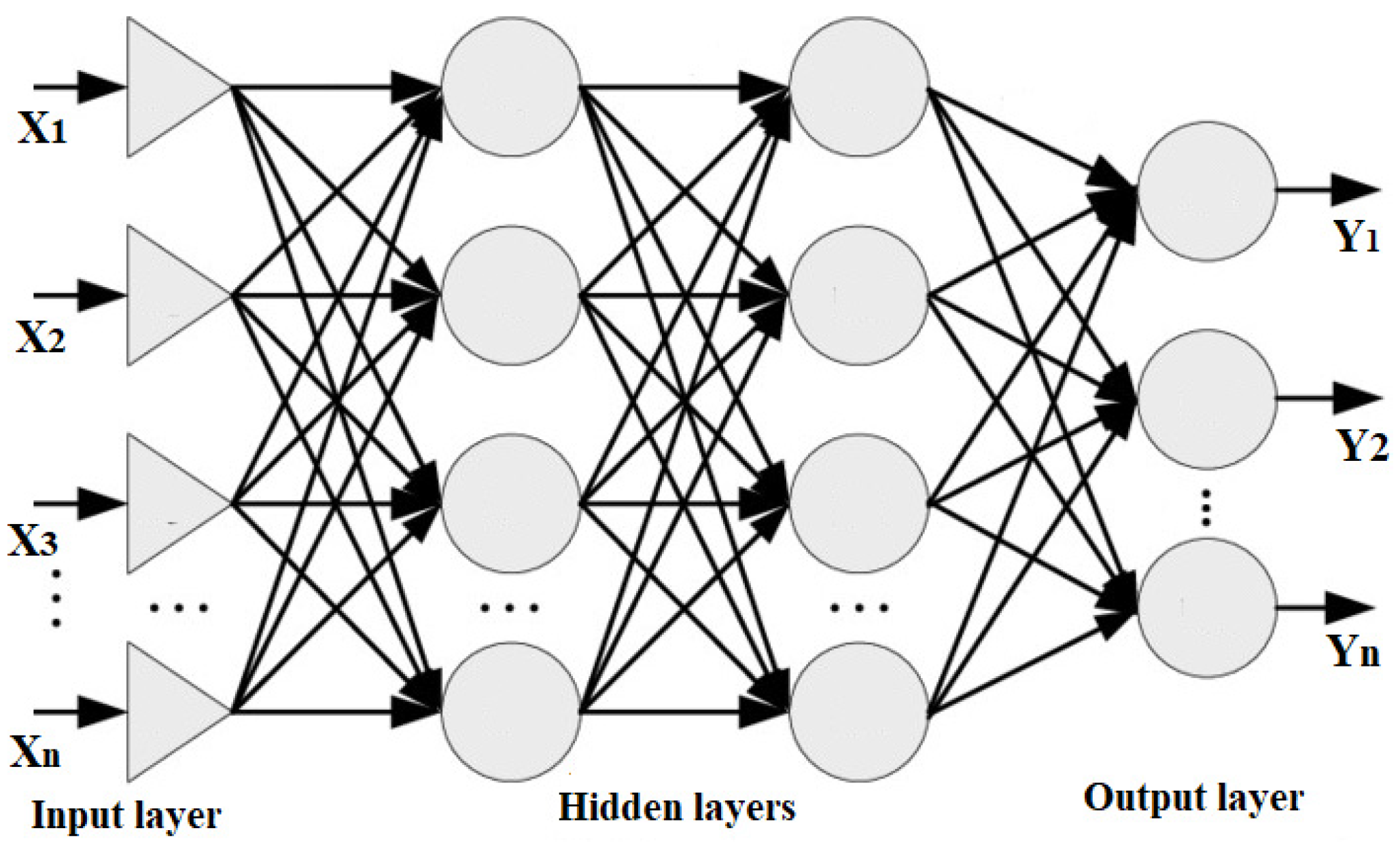
An artificial neural network having numerous layers between the input and output layers is known as a deep neural network (DNN). Data flows via neural networks in two ways: the multilayer perceptron (MLP) model is used to predict the output for the provided data in forwarding propagation, and the model updates its parameters in backpropagation based on the prediction error. Figure 6 depicts the MLP architecture utilized for fault classification. The feature vector is introduced into the model, and the output of the first and subsequent hidden layers is given by the Equations below.
h 1 = σ   [ W 1 . ( x ) + b 1 ]
h i = σ   [ W 1 i . ( h i 1 ) + b i ]
Here i denotes the layer index, and the activation function is represented by σ . The x-dimension is equal to 3636 × 9. Each column indicates a feature of the neural net, as stated earlier. Following is the output of the MLP:
y = σ s o f t   ( h o u t )
Each layer is assigned an activation function based on the hyperbolic tangent (tanh). In order to identify the specific nature of a PV array fault, the output layer employs the Softmax activation function.

3.3.2. LSTM

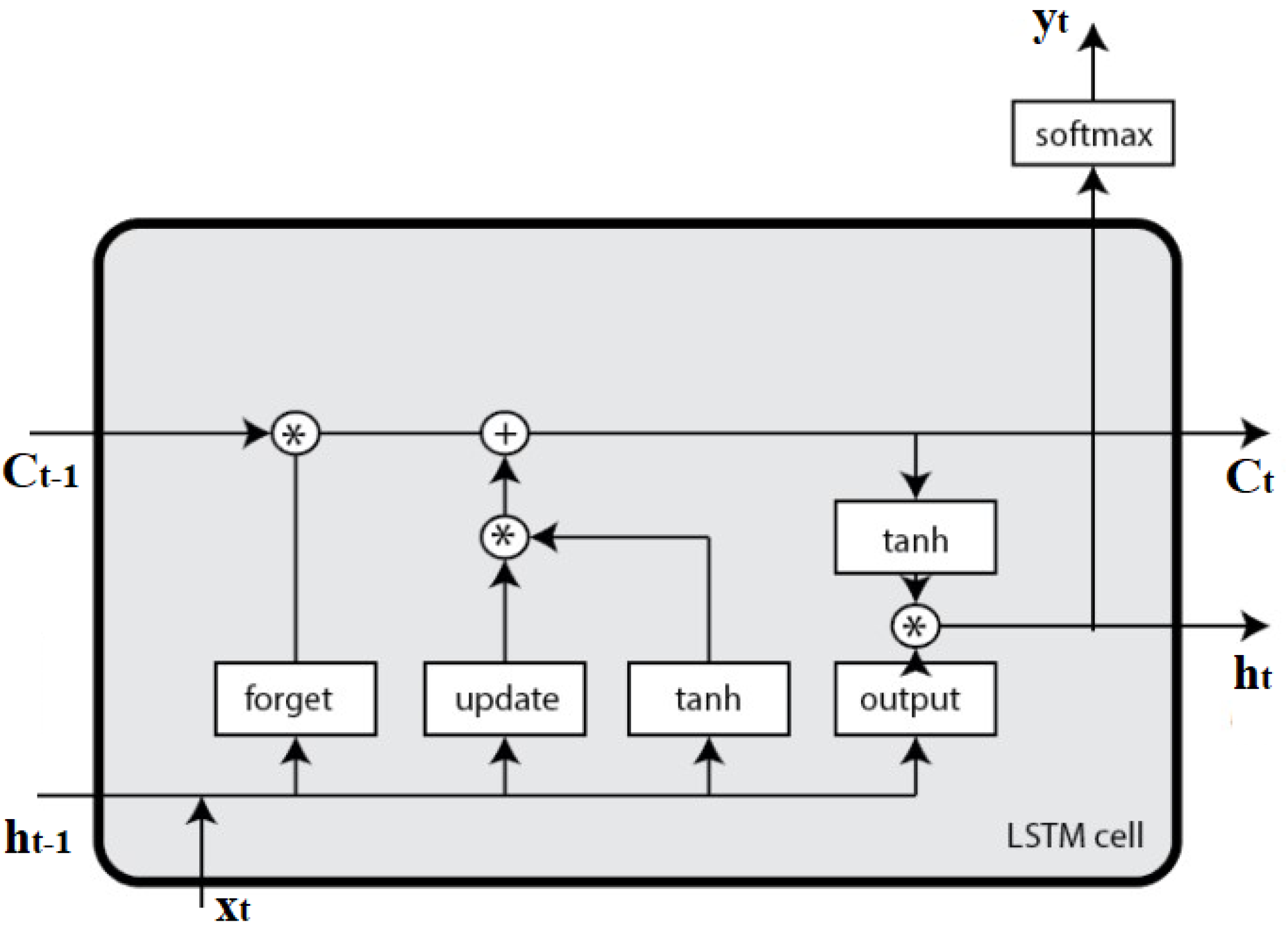
Hochreiter et al. introduced LSTM networks, an updated recurrent neural network (RNN) that aimed to capture long-term reliance in data sequences to counter the gradient vanishing issue [29]. The local closest activation modifies a regular RNN’s hidden state, sometimes referred to as short-term memory. On the other hand, the network weights are adjusted by computations performed throughout the extended data sequence, which is referred to as long-term memory. In order to maintain data integrity over extensive ranges, LSTM is equipped with an activation state that is used as a weight. Figure 7 depicts the basic structure of a single neuron in an LSTM neural network. The computation formulas for LSTM neurons are as follows:
I t = σ   [ W x i   ( x t ) + W h i   ( h t 1 ) + W c i   ( c t 1 ) + b i ]
F t = σ   [ W x f   ( x t ) + W h f   ( h t 1 ) + W c f   ( c t 1 ) + b f ]
O t = σ   [ W x o   ( x t ) + W h o   ( h t 1 ) + W c o   ( c t ) + b o ]
h t = o t tanh ( c t )
In this case, I, f, o, and c stand in place of the input gate, the forget gate, the output gate, and the neuron memory cell, respectively. The neuron’s input and output are indicated by the values of x and h, respectively. Whereas σ , W, and b denote the excitation function, weight coefficient matrix, and bias matrix, respectively. In this study, x refers to input features compromising of PV system dataset, while h represents predicted output based on the type of PV fault.

3.3.3. Bidirectional LSTM

Bidirectional LSTM, also called “Bi-LSTM”, is a specific RNN. The LSTM predicts follow-up information. To improve prediction accuracy, however, the Bi-LSTM model may simultaneously learn time-correlated info through both forward and backward directions. Figure 8 depicts the architecture of the Bi-LSTM. Forward and backward LSTM hidden vectors at a time are denoted by h f and h f , respectively. The h f and h f are independent and only relate to their LSTM layers. The forward layer shows the unidirectional flow from input to hidden to output [44]. Connecting the two hidden states allows us to compute the final Bi-LSTM’s prediction y t , as depicted in Figure 8. The process can be described with the help of Equations (10)–(12) as follows:
h f = L S T M   ( x t ,   h f ( t 1 ) )
h b = L S T M   ( x t ,   h b ( t + 1 ) )
y t = σ   [ W h y f   ( h f ) + W h y b   ( h b ) + b y ]
where LSTM (-) represents LSTM network, both the forward and backward LSTM layers’ weights at time t are denoted by W h y f and W h y b , respectively. The activation function is denoted by σ , while the bias of the output layer is indicated by b y .

3.4. Development of Base Learners and Meta-Learner for Proposed Algorithm

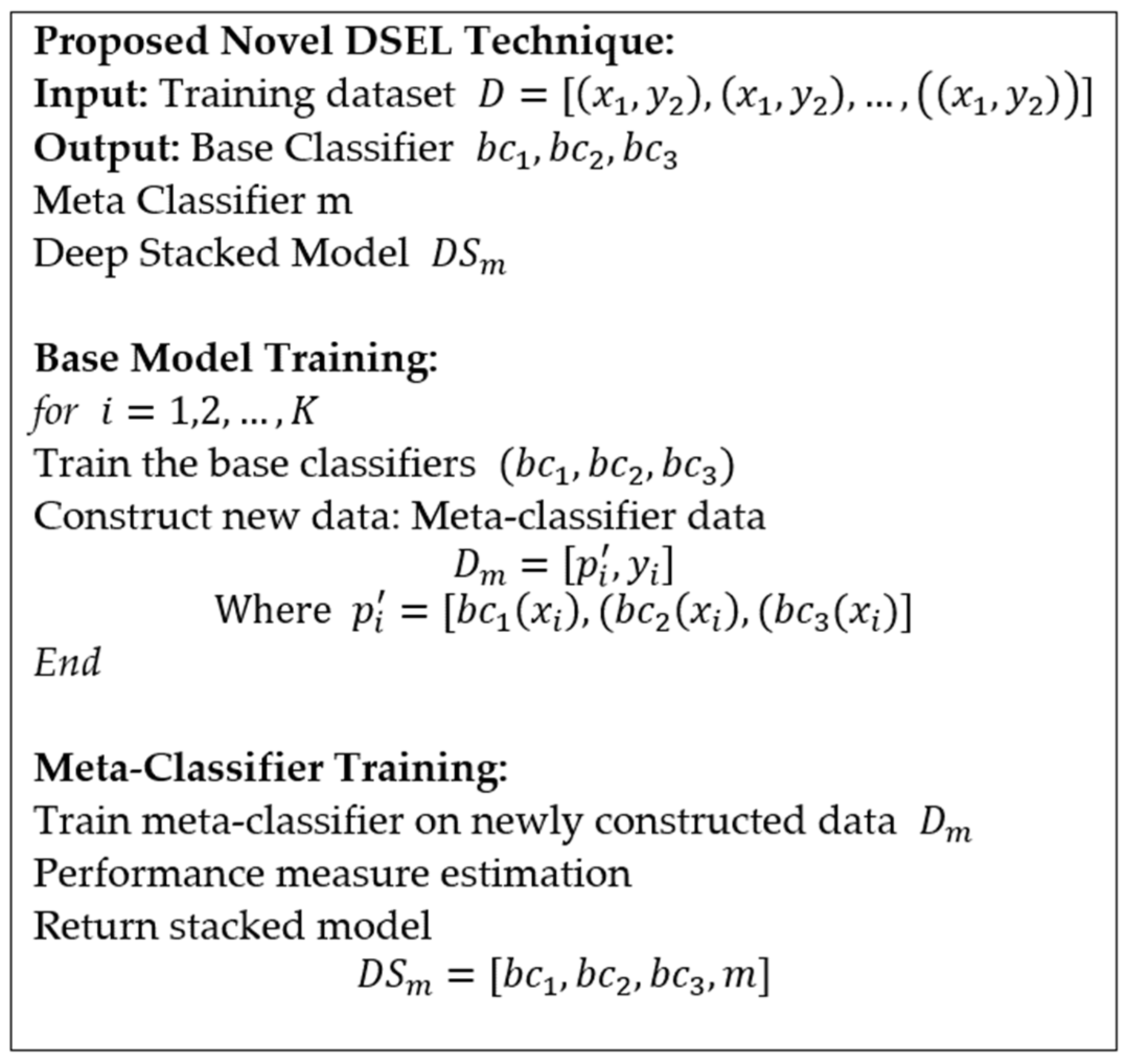
For the practical development of the DSEL algorithm for fault detection strategy, the architecture of base learners (DNN, LSTM, and Bi-LSTM) and meta-learner model (MLR) are briefly explained in the following section. Figure 9 illustrates a pseudocode for the proposed DSEL approach.

3.4.1. Architecture of DNN

This subsection provides an overview of the DNN model’s internal structure, developed with the Keras deep-learning library. It comprises an input layer that accepts various input features, two hidden layers with numerous nodes per layer and a relu activation function, and an output layer with six neurons and a softmax activation function, which directly links to the target value the model attempts to predict. The grid search technique is used to determine the number of hidden layers. The 1–5 hidden layers are tested. Ultimately, two hidden layers are the best option and work well on the test dataset because the data is less complicated and has fewer parameters. Hence, DNN’s base model has two hidden layers and runs for 125 epochs with a batch size of 16.

3.4.2. Architecture of LSTM

An overview of the LSTM model’s design methodology, developed with the Keras deep-learning package, is introduced in this part. The sequential API framework is utilized to initialize the model variable. The first layer is an embedding layer, followed by two LSTM layers that provide the recurrent segment with a default tanh activation function. In order to provide an efficient regularization strategy that avoids over-fitting and enhances generalization performance, a dropout layer is additionally added to the network. The dropout rate is chosen as 0.5, which means that 50% of the layers will be removed. After that, there is a dense layer with six outputs. The softmax activation function uses a number between 0 and 5 to demonstrate the orientation of the fault class. Afterward, a widely-used Adam optimizer tool is utilized to assemble our model. Then, the model is adjusted to use a batch size of 32 and run for 100 epochs.

3.4.3. Architecture of Bi-LSTM

Bi-LSTM refers to the method by which a neural network may be constructed to store sequence data in either the forward (from present to the future) or backward (from the future to the past) direction. In this section, the Keras deep-learning framework is examined for use in the architecture of the Bi-LSTM model. The model variable is initialized through the sequential API framework. The Bi-LSTM layer is added to a conventional neural network using Keras. Keras of tensor flow offers a new class (bidirectional) to develop Bi-LSTM. A dropout layer of 0.4 is added to the network to provide an efficient regularization method that prevents over-fitting and improves generalization performance. Following that, a dense layer with six outputs depicts an orientation toward a faulty class using a number between 0 and 5 as the softmax activation function. Afterward, the Adam optimizer tool is utilized to assemble the Bi-LSTM model. The model is then adjusted to run for 75 epochs with a batch size of 32.

3.4.4. Architecture of Multinomial Logistic Regression

The meta-learner model is generally simple, allowing for an easy interpretation of the base model’s predictions. Consequently, linear models are frequently employed as the meta-model—for example, logistic regression for the prediction of class labels in classification tasks and linear regression for predicting a numeric value in regression problems. To enhance diversity, multiple meta-learner models (logistic regression, decision trees, AdaBoost, SVM, and XGBoost) are examined for the research in this study. Unlike other learning algorithms, multinomial logistic regression (MLR) outperforms them on all datasets. Since the meta-learner received the results from the output of distinct base learner models, this study uses a forward propagation network to establish the network’s topology, with the Adam method chosen by the optimizer and a Softmax function serving as the final output layer.

3.5. Training and Testing

The operational dataset of the PV system is distributed into training and testing datasets after the data preprocessing and feature engineering phases are completed. The training dataset comprises seventy percent of the original data, while the test dataset accounts for thirty percent of the overall data. Section 2 contains information on the number of samples in each fault category. Using k-folds cross-validation, DNN, LSTM, and Bi-LSTM base learners are trained on distinct folds of the training data. The k-fold cross-validation also offers an unbiased assessment of the model’s performance. K-fold cross-validation training reduces variance more effectively than a single hold-out model, which might be necessary when limited data is available. K-fold divides the data into k equal-sized chunks. Five folds of cross-validation are used to validate the base learner models. The first four folds are utilized for training the models during the first iteration, while the last one is used to test the model’s performance. The second to last fold is used for model testing in the next iteration, whereas the remaining folds are used for training. This procedure is performed five times to get predictions for each of the five test folds. In this scenario, the cross-validation stacking structure generates second-level data for multinomial logistic regression (MLR) meta-learner. Stacking is similar to cross-validation in that it solves two critical problems: collecting varied regions where each model works best and producing out-of-sample predictions. The primary concept of deep ensemble stacking is to add weights ( w 1 ,…, w i ) to the predictions ( p 1 ,…, p i ) made by the base models, as shown in Equation (13).
f s ( x ) = i = 1 n ( w i p i )
The meta-learner is used to train with predictions from the base learners’ algorithms to discover the optimal way to merge the predictions for the output. The meta classifier is primarily responsible for the stacking algorithm’s generalization ability, which can differentiate whether each base classifier executes well or badly. The MLR is used as a meta-classifier because it is capable of more rapid computing and can make accurate predictions using higher-dimensional space with smaller training datasets. The ultimate predictions are acquired utilizing the test dataset after training the base learners and the meta-learner. The description of the whole algorithm is shown in Figure 9. The training data D is used to train each base learning algorithm ( b c 1 ,   b c 2 , b c 3 ), and the cross-validated predicted values are obtained from each algorithm. A new ( m p ) matrix is created by combining the p i cross-validated predicted values from each algorithm. The meta-learner training data consists of this ( m p ) matrix and the initial response vector y i . This new metadata D m is used to train the meta-learning algorithm. The stacked ensemble model D S m is derived from the base and meta-learning models, which are then utilized to generate the test dataset prediction. The data partition of the proposed DSEL model used in the training and testing process is depicted in Figure 10.

3.6. Development Setup

The simulated PV system is designed in a MATLAB Simulink environment and is used for data collection, and it is powered by an Intel Core(TM) i5-3210M processor having a frequency of 2.70 GHz and 8 GB of RAM. The proposed DSEL algorithm used Python in an open-source, cross-platform IDE, called Jupyter Notebook. Keras was utilized to develop LSTM and Bi-LSTM due to its extensibility and modularity. Keras runs on TensorFlow to expedite deep neural network exploration. Google’s TensorFlow is an open-source platform for differential programming. Finally, the efficacy and superiority of the proposed DSEL algorithm are validated compared to other existing contemporary fault-diagnosis techniques. Observations indicate that the proposed approach outperforms previous techniques, attaining 98.7% fault detection accuracy for noiseless and 95.77% for noisy data. According to the results, the DSEL technique enhances classification performance while retaining a dominant generalization potential for fault detection.

4. Results Evaluation and Discussion

Performance evaluation is important to examine and investigate the effectiveness of any technique. This section presents the outcomes achieved by using the proposed DSEL fault-diagnostic algorithm. The optimal set of hyperparameters for each model of the proposed DSEL fault-diagnosis algorithm is determined via a grid search. Machine-learning models rely heavily on hyperparameters, which regulate the strength of training algorithms and are, thus, imperative to the success of these models. The tested grids’ hyperparameters and optimal parameters for the trained base learners and meta-learner models are listed in Table 3. After each model was trained, its generalization ability was checked using its test data. This research takes into account five distinct faulty conditions and one no-fault condition, namely, open circuit (OC-Fault), short circuit (SC-Fault), bridge (B-Fault), partial shading (PS-Fault), degradation (D-Fault), and no-fault (No-Fault) conditions. The findings of the proposed DSEL approach are provided and compared with eight other contemporary fault classification techniques, such as probabilistic neural network (PNN), Bi-LSTM, LSTM, DNN, ANN, Gradient Boost, Adaboost, support vector machine (SVM), and Random forest (RF). The proposed DSEL algorithm provides reliable and accurate PV-fault diagnostics for noiseless and noisy data.

4.1. Performance Measure Based on Noiseless Data

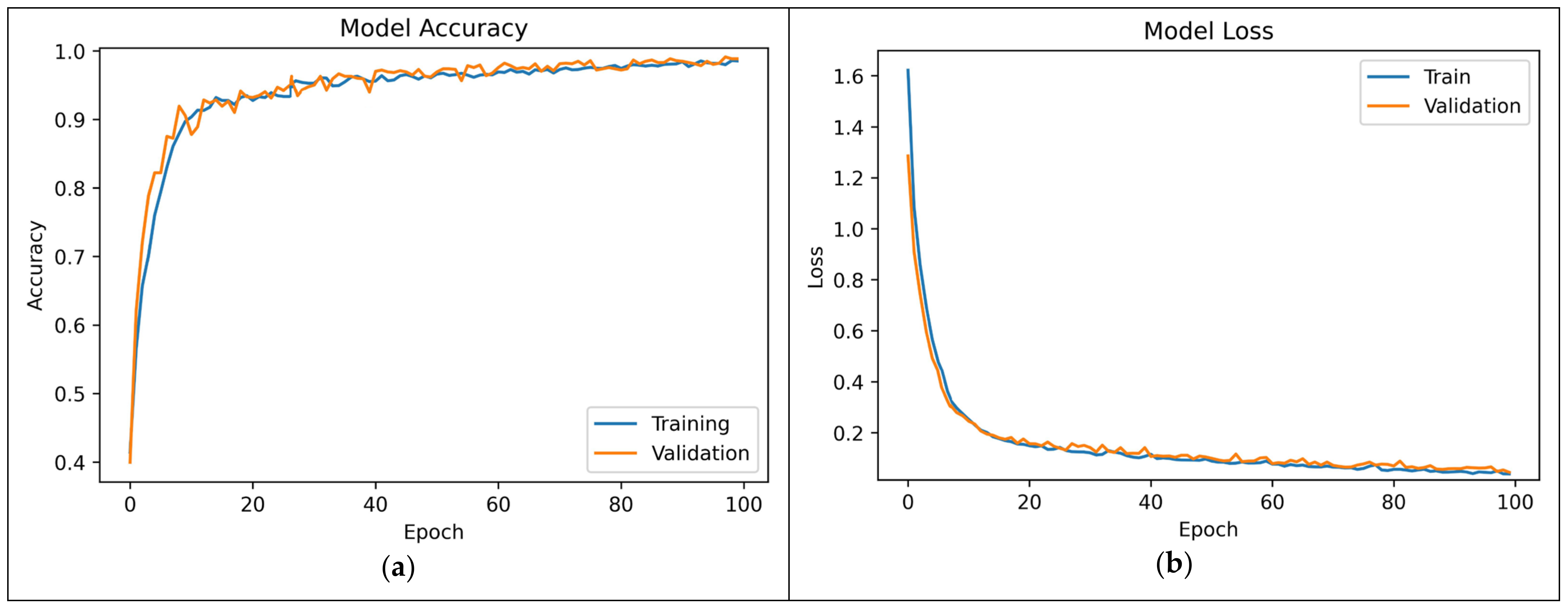
This section discusses the performance measurements required to evaluate and analyze the proposed DSEL algorithm on a noiseless dataset. This paper utilizes accuracy and loss as evaluation criteria to track training and validation performances. Accuracy is the percentage of data samples with correctly predicted labels. Loss is an error that measures how good the model’s output is compared to the ground truth label. Too many epochs overfit the training dataset, while too few underfit the model. The DSEL model was trained for 25–125 epochs to eliminate overfitting and improve generalization. After 100 epochs, model accuracy saturates, and validation error increases, which may indicate overfitting. Thus, the ideal epoch is chosen as 100. The progression of accuracy in training and validation throughout the training epochs for noiseless datasets is depicted in Figure 11a. When examining Figure 11a, it is clear that the overall accuracy improves over time and eventually reaches approximately 98.62%. The suggested DSEL algorithm model obtains many better-optimized parameters with each subsequent epoch until convergence, as evidenced by the constant improvement in training accuracy. Figure 11a illustrates that progressive gains in training and validation accuracy show no variance problem with the trained model. This lack of variance improves the model’s generalization to test data. Figure 11b shows the progression of training and validation losses over epochs. The better the model, the lower the convergence loss. A lower loss value at convergence indicates a more accurate model. Training and validation losses decreased simultaneously and converged around 0.056.
Metrics, such as accuracy, precision, sensitivity (Recall), and F-Score, further evaluate the proposed DSEL method’s overall behavior. Equations (14)–(17) provide a representation of these metrics [33]:
A = ( t p o + t n o ) ( t p o + t n o + f p o + f n o )
P = ( t p o ) ( t p o + f p o )
R = ( t p o ) ( t p o + f n o )
F S = 2 ( R P ) ( R + P )
Accuracy, precision, recall, and F-Score are denoted by A ,   P ,   R , and F S , respectively. The t p o displays the amount of faulty data samples classified as faulty conditions. The t n o indicates the quantity of identified normal data samples and symbolizes a normal condition. The f p o defines a collection of normal data samples that represent a normal condition. The f n o shows the quantity of faulty data samples that are classified as normal.
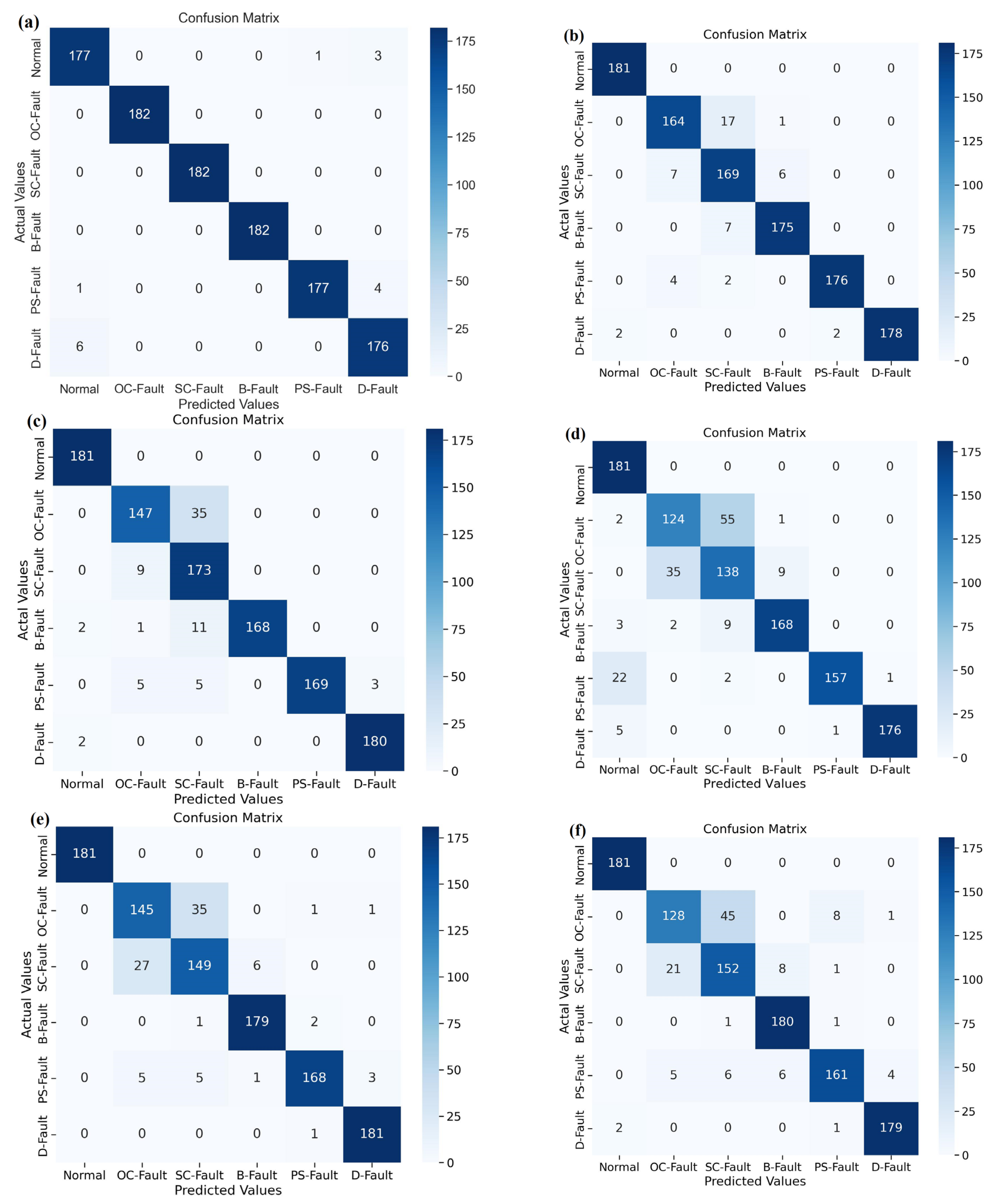
An analysis of the various models presented in a confusion matrix is shown in Figure 12. The entries in the confusion matrix are discussed below. The confusion matrix’s sum of entries along a row indicates samples from a certain class in the testing dataset. From Figure 12a, the proposed DSEL algorithm for fault diagnosis categorized 177 testing data samples from the normal (no-fault) category as belonging to the normal (no-fault) category, one data sample from the PS-Fault category as belonging to the normal (no-fault) category, and six data samples from the D-Fault category as belonging to the normal (no-fault) category. The 182 data samples from the OC-Fault category belong to the OC-Fault category. The 182 data samples from the SC-Fault category belong to the SC-Fault category. The 182 data samples from the B-Fault category belong to the B-Fault category. The 177 data samples from the PS-Fault category belong to the PS-Fault category; one sample from the normal (no-fault) category belongs to the PS-Fault category. Finally, the 176 data samples from the D-Fault category belong to the D-The fault category, 3 data samples from the normal (no-fault) category belong to the D- Fault category, and 4 data samples from the PS-Fault category belong to the D-Fault category. Taking into consideration the indications, Figure 12a demonstrates that the fault-diagnosis accuracy of the proposed DSEL algorithm for Normal, OC-Fault, SC-Fault, B-Fault, PS-Fault, and D-Fault is 97.79%, 100%, 100%, 100%, 97.26%, and 96.7%, respectively. The overall accuracy of the proposed DSEL methodology is approximately around 98.625%. The proposed method leads to accurately identifying observations with minor misclassification errors. The suggested DSEL approach has an outstanding classification impact and can greatly enhance the fault-diagnosis capabilities of PV arrays.
In addition, the fault-diagnostic results obtained using the suggested DSEL algorithm are compared to other AI-based fault-diagnosis techniques using the abovementioned metrics. Table 4 also depicts the accuracy, precision, sensitivity (recall), and F1-score achieved by various fault-diagnostic algorithms. Similarly, the confusion matrix obtained by utilizing the Bi-LSTM and LSTM algorithms is presented in Figure 12b,c. The accuracy achieved using Bi-LSTM and LSTM algorithms are around 95.66% and 93.35%, respectively, as mentioned in Table 4. Furthermore, the confusion matrices shown in Figure 12d,e provide insight into the efficacy of PNN and DNN algorithms. According to Table 4, the accuracy achieved by the PNN and DNN algorithms is approximately 92.11 percent and 91.89 percent, respectively. Similarly, the performance of ANN and Gradient Boost algorithms is depicted in the confusion matrix that is shown in Figure 12f,g. Table 4 shows that the accuracy of the ANN and Gradient Boost algorithms is about 90.37% and 87.83%, respectively. Correspondingly, Figure 12h,i depicts a confusion matrix that sums up the results of AdaBoost and SVM algorithms. As shown in Table 4, the accuracy attained using the AdaBoost and SVM algorithms is approximately 85.26% and 82.75%, respectively. In addition, a bar chart depicting performance metrics, such as accuracy, precision, recall, and F1-score for several fault-diagnostic algorithms, is provided in Figure 13. The SVM algorithm has demonstrated the lowest percentage of performance across all metrics. However, the proposed DSEL approach outperforms all metrics and has exceptional fault-diagnosis capabilities in PV arrays with a noiseless dataset.
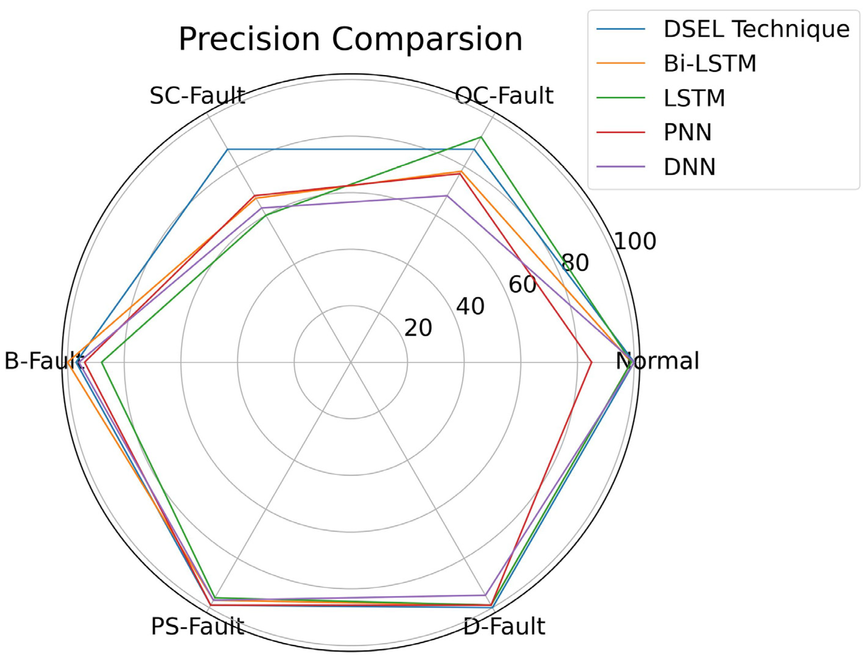
To further extend the validity of the proposed DSEL fault-diagnosis algorithm, a comparison can be made regarding precision among different fault-diagnosis algorithms (Bi-LSTM, LSTM, PNN, and DNN) with the help of a radar plot. As illustrated in Figure 14, the precision of the proposed DSEL methodology for normal, OC-Fault, SC-Fault, B-Fault, PS-Fault, and D-Fault is 96.12%, 100%, 100%, 100%, 99.27%, and 96.04%, respectively. Under the noiseless dataset, the suggested DSEL methodology’s overall precision is approximately 98.57%. Compared to other fault-diagnosis algorithms, Bi-LSTM, LSTM, PNN, and DNN achieve overall precisions of about 95.83%, 94.01%, 92.63%, and 91.97%, respectively. Consequently, it can be observed from radar plot analysis in Figure 14 that the proposed DSEL approach outperforms other strategies regarding PV-fault detection precision under a noiseless dataset.

4.2. Performance Measurements Based on Noisy Dataset

Performance measurements are necessary to determine how well a classifier works and analyze its effectiveness under different conditions. Due to the absence of noise (i.e., disturbance), the dataset depicted in Section 4.1 is considered noiseless. Any data collected by sensing and measuring instruments in real-world circumstances will likely have some background noise. For this reason, an effort has been put into generating noisy data by adding noise to previously noiseless data to approximate real-world situations as closely as possible. The approach to noise signal creation adopted in [34] is represented in Equation (18).
D = A i + B i r a n d o m ( 1 , N )
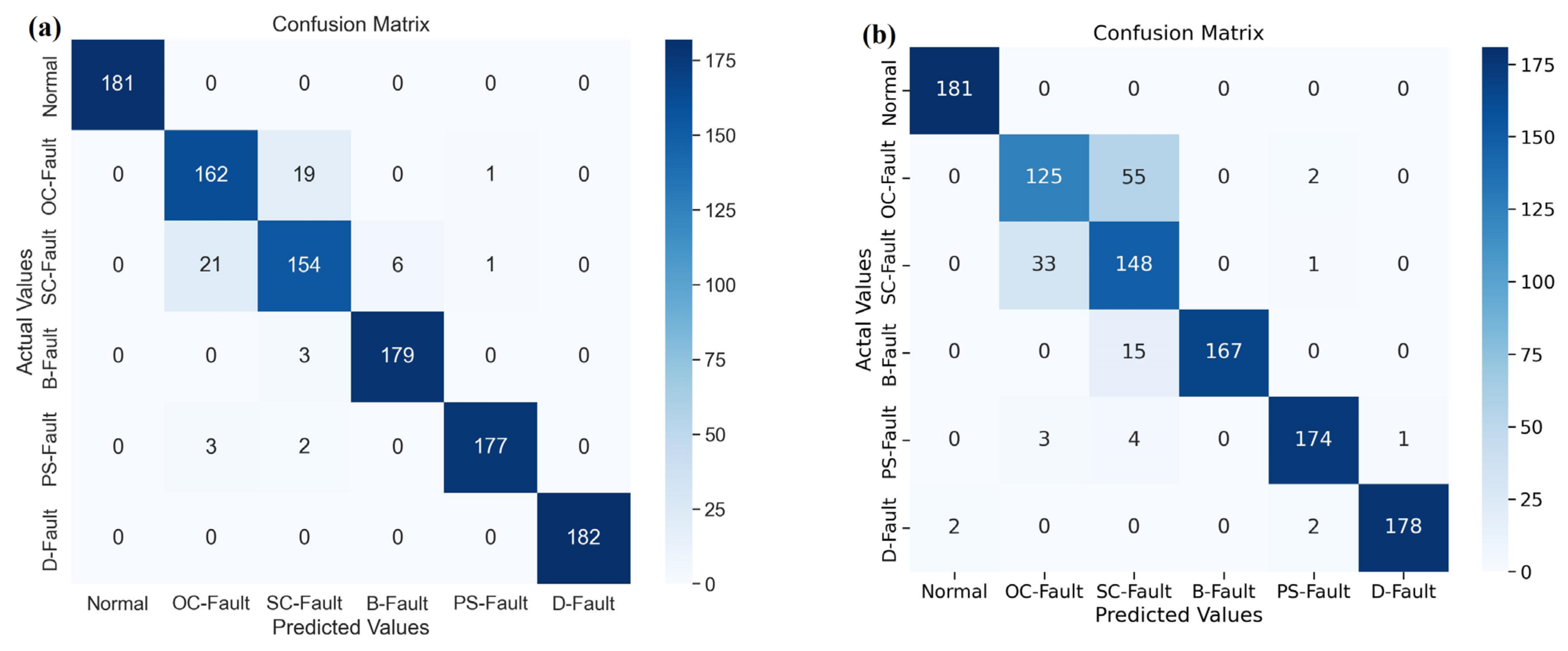
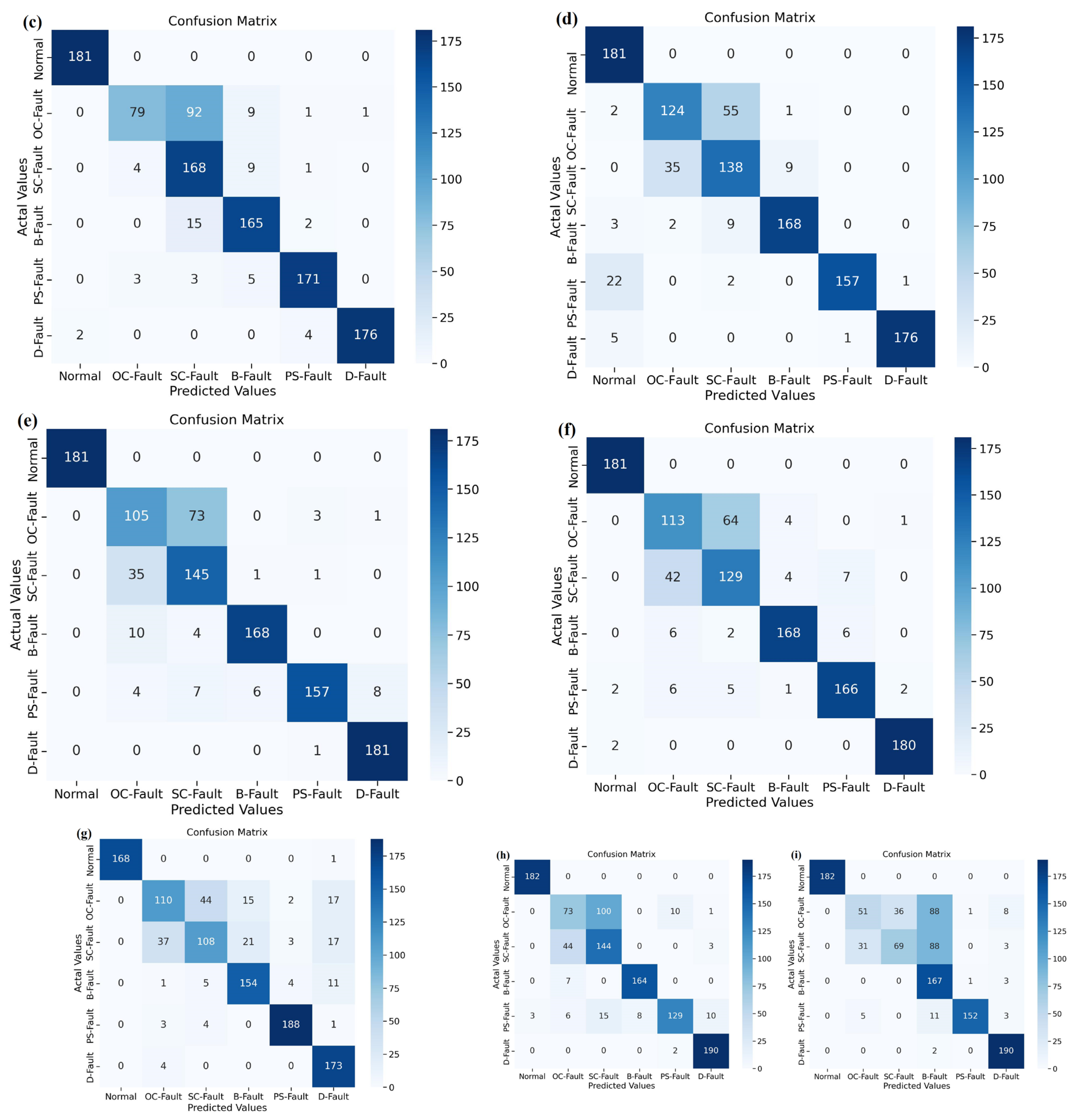
where A i and B i denote the mean and intensity of the disturbing pulse, random is the noisy default function, and N represents the size of the disturbing signal. The distribution of noise generated for data samples of irradiance, temperature, voltage, current, and power is based on the following range of random noise amplitudes: B i r = ( 0.25 2 ) ;   B t = ( 0.25 2 ) ;   B v = ( 2 5 ) ;   B i = ( 0.2 1.5 ) ;   and   B p = ( 0.4 7.5 ) . Figure 15 displays a confusion matrix that evaluates the various PV-fault-diagnostic techniques in the context of a noisy dataset. The number of entries across a row of the confusion matrix represents the number of samples from a specific class in the tested dataset. Figure 15a demonstrates that the proposed DSEL fault-diagnosis algorithm under a noisy dataset classified 181 testing data samples from the normal (no-fault) category as belonging to the normal (no-fault) category, the 162 data samples from the OC-Fault category as belonging to the OC-Fault category, 21 data samples from the SC-Fault category as belonging to the OC-Fault category, three data samples from the PS-Fault category as belonging to the OC-Fault category, the 154 data samples from the SC-Fault category as belonging to the SC-Fault category, 19 data samples from the OC-Fault category as belonging to the SC-Fault category, three data samples from the B-Fault category as belonging to the SC-Fault category, two data samples from the PS-Fault category as belonging to SC-Fault category. The 179 data samples from the B-Fault category belong to the B-Fault category, and six from the SC-Fault category belong to the B-Fault category. The 177 data samples from the PS-Fault category belong to the PS-Fault category, one from the OC-Fault category belongs to the PS-Fault category, and one from the SC-Fault category belongs to the PS-Fault category. Lastly, the 182 data samples from the D-Fault category belong to the D-Fault category. Taking into consideration the indications, Figure 15a demonstrates that the fault-diagnosis accuracy of the proposed DSEL approach technique under noisy dataset conditions for Normal, OC-Fault, SC-Fault, B-Fault, PS-Fault, and D-Fault is 100%, 89.01%, 84.61%, 98.35%, 97.25%, and 100%, respectively. The proposed DSEL algorithm’s overall accuracy is around 94.87% under noisy datasets, as depicted in Table 4. The proposed DSEL approach has an outstanding classification impact under noisy dataset conditions and can greatly enhance the fault-diagnosis capabilities of PV arrays.
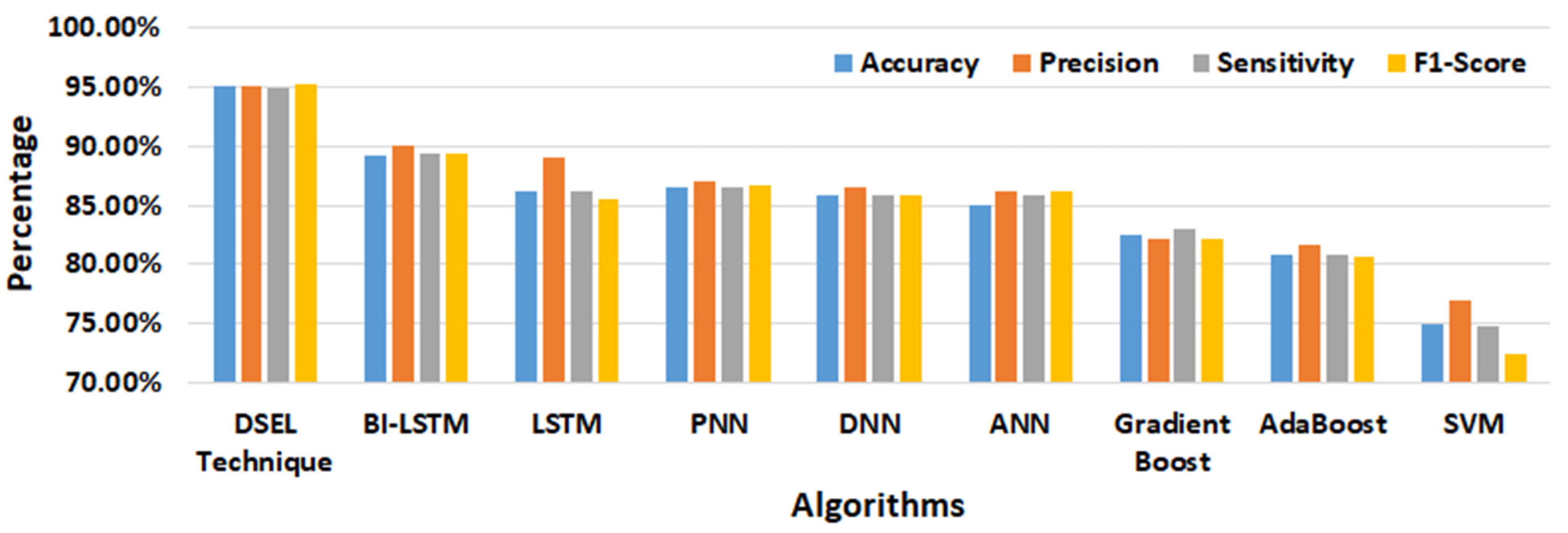
The performance of the proposed DSEL algorithm is compared to that of other PV-fault classification AI-based algorithms by using the metrics mentioned above. Table 5 also depicts the accuracy, precision, sensitivity (recall), and F1-score achieved by various fault-diagnostic algorithms under noisy dataset conditions. Similarly, the confusion matrix obtained by utilizing the Bi-LSTM and LSTM algorithms is presented in Figure 15b,c. The accuracy achieved using Bi-LSTM and LSTM algorithms are around 89.18% and 86.15%, respectively, as mentioned in Table 5. Likewise, the confusion matrices shown in Figure 15d,e depicts the efficacy of PNN and DNN. According to Table 5, the accuracy achieved by the DNN and ANN algorithms is approximately 86.53 percent and 85.88 percent, respectively. Similarly, the performance of ANN and Gradient Boost is depicted in the confusion matrix that is shown in Figure 15f,g, respectively. Table 5 shows that the accuracy of the ANN and Gradient Boost algorithms is about 84.98% and 82.58%, respectively. Similarly, Figure 15h,i depict a confusion matrix that sums up the results of the AdaBoost and SVM. As shown in Table 5, the accuracy attained using the AdaBoost and SVM algorithms is approximately 80.84% and 74.87%, respectively. Furthermore, Figure 16 compares the performance of several PV-fault-diagnostic algorithms under noisy dataset conditions using a bar chart depicting accuracy, precision, recall, and F1-score results. The SVM classifier has shown the least performance in all metrics. However, the proposed DSEL algorithm shows remarkable results in all metrics and has outstanding fault-diagnosis capabilities in PV arrays under a noisy dataset.
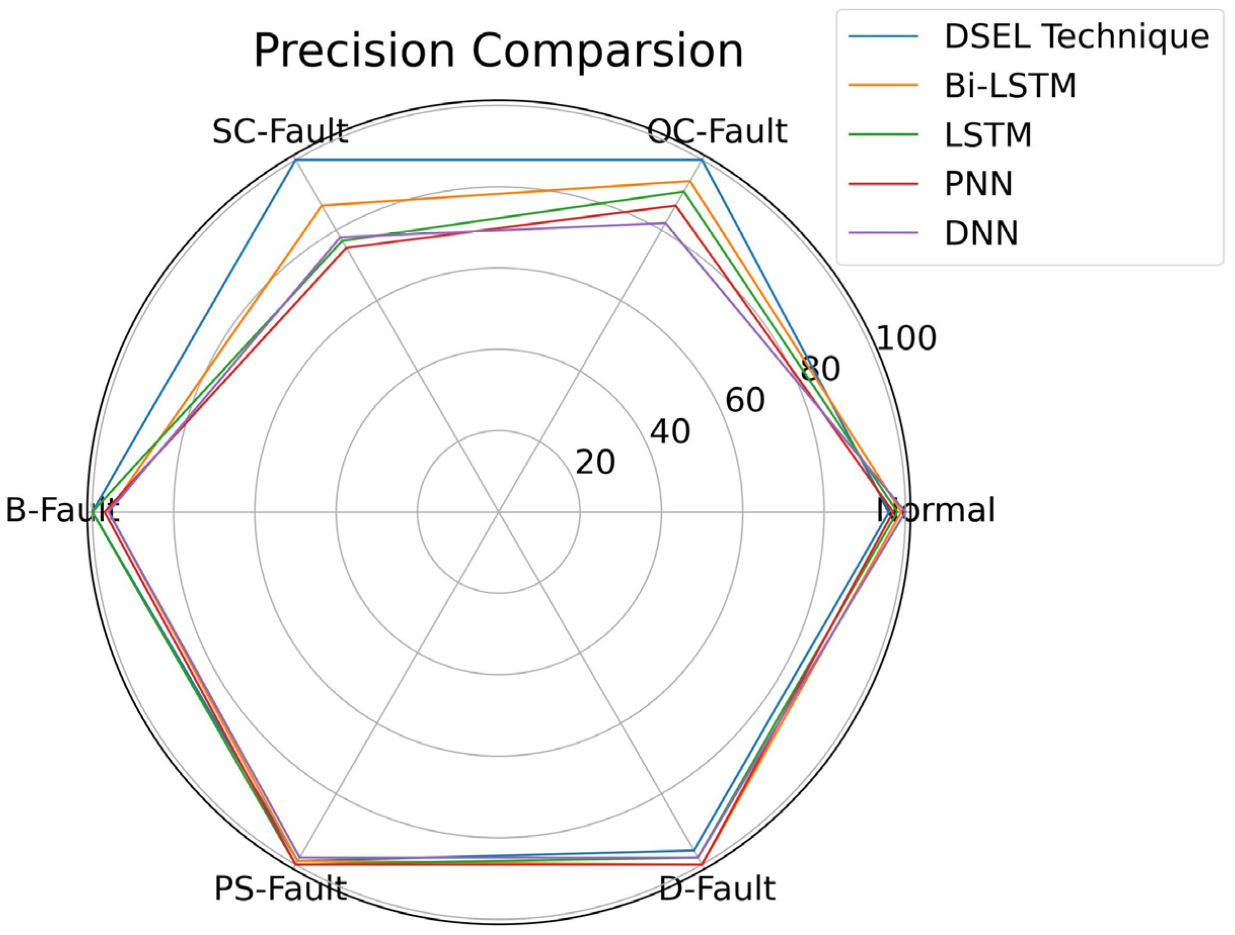
To further enhance the applicability of the suggested fault-diagnostic technique on noisy datasets, a comparison of other techniques’ precision can be made, including Bi-LSTM, LSTM, PNN, and DNN. In this case, the radar plot is used to create a precision comparison. Figure 17 shows that the proposed DSEL method achieves 100% accuracy for normal, 87.43% for OC-Fault, 97.13% for SC-Fault, 97.07% for B-Fault, 99.02% for PS-Fault, and 100% accuracy for D-Fault conditions. The average precision of the proposed DSEL methodology is roughly 95.10% when using the noiseless dataset. Bi-LSTM, LSTM, PNN, and DNN obtain average precisions of 90.11%, 89.08%, 87.03%, and 86.50%, respectively, compared to other fault-diagnostic techniques. As a result, radar plot analysis shows that the proposed approach supersedes other competing strategies in terms of precision-detecting PV faults under noisy dataset conditions.

5. Conclusions

This article presents the deep stack-based ensemble learning (DSEL) approach, which comprises DNN, LSTM, and Bi-LSTM deep-learning models. Due to the inclusion of strong base learner models, the proposed DSEL approach significantly outperforms the individual deep-learning techniques. Multinomial logistic regression is used as a meta-learner to combine the predictions of base models, leading to improved PV array diagnosis. The meta-learner model also decreases bias and variance by fixing the flaws in the base learner models and selecting their best features for the final prediction. The PV array model is designed to examine faults. The proposed DSEL algorithm pertained to a PV system’s correlation dataset. The dataset is typically nine parameters extracted as data attributes, directly or indirectly affected by PV faults, which serve as a representative dataset. This research study is the first thorough, significant, and useful comparison of PV-fault detection that considers six different scenarios (five faulty scenarios along with the no-fault scenario) and a consistent dataset for comparing the proposed approach with those of prior researchers. The suggested DSEL approach has even been benchmarked using Bi-LSTM, LSTM, PNN DNN, ANN, Gradient Boost, AdaBoost, and SVM algorithms. Observations illustrate that the suggested method exceeds prior techniques, achieving detection accuracy of 98.62% fault for noiseless and 94.87% for noisy datasets. The results demonstrate that the proposed DSEL methodology enhances classification accuracy, thus keeping the dominant generalization potential for detecting PV faults. Therefore, the proposed DSEL technique approach performs admirably and detects PV array system faults more effectively. This research work might guide future studies to enhance reliability and fault-diagnostics capabilities in PV systems.
To summarize, some limitations and directions for future study of fault diagnosis in PV systems are listed as follows: (i) The arc faults are not considered in this research analysis. The arc faults can be investigated in future research to improve the efficiency of the proposed approach; (ii) More research is needed in this seminal domain to thoroughly determine the upsides and downsides of deep-learning paradigms. This is because deep-learning models come in various forms (CNN, RBM, DBP, AE, and so on) utilized to select better efficient methods for fault diagnosis; (iii) Another factor to consider when selecting the base models is the possibility of a trade-off between prediction accuracy and computational time; (iv) Experimental trials are also planned on actual PV systems to gather the dataset for faulty and non-faulty conditions and further investigate the validity of the proposed approach in the near future; (v) Furthermore, it plans to establish an intelligent remote sensing-based monitoring framework for fault diagnostics in PV systems.

Author Contributions

Conceptualization, E.L. and F.-Y.W.; methodology, E.L. and G.X.; software, E.L. and M.A.K.; validation, E.L., W.U.R. and M.A.K.; formal analysis, L.Z. and T.S.T.; investigation, T.S.T. and W.U.R.; resources, G.X. and F.-Y.W.; data curation, E.L. and M.A.K.; writing—original draft preparation, E.L.; writing—review and editing, F.-Y.W., G.X., L.Z. and W.U.R.; visualization, L.Z., W.U.R. and M.A.K.; supervision, F.-Y.W. and G.X.; project administration, F.-Y.W. and G.X.; funding acquisition, F.-Y.W., G.X. and L.Z. All authors have read and agreed to the published version of the manuscript.

Funding

This research was funded by the National Natural Science Foundation of China under Grants U1909204 and U19B2029, Key Industrial Innovation Chain Project of Shaanxi Province Key R&D Program of China, grant number 2020ZDLGY10-04, and the APC was funded by 2020ZDLGY10-04.

Conflicts of Interest

The authors declare no conflict of interest.

References

  1. Wang, L.; Lodhi, E.; Yang, P.; Qiu, H.; Rehman, W.U.; Lodhi, Z.; Tamir, T.S.; Khan, M.A. Adaptive Local Mean Decomposition and Multiscale-Fuzzy Entropy-Based Algorithms for the Detection of DC Series Arc Faults in PV Systems. Energies 2022, 15, 3608. [Google Scholar] [CrossRef]
  2. Aghaei, M.; Fairbrother, A.; Gok, A.; Ahmad, S.; Kazim, S.; Lobato, K.; Oreski, G.; Reinders, A.; Schmitz, J.; Theelen, M.; et al. Review of degradation and failure phenomena in photovoltaic modules. Renew. Sustain. Energy Rev. 2022, 159, 112160. [Google Scholar] [CrossRef]
  3. Hojabri, M.; Kellerhals, S.; Upadhyay, G.; Bowler, B. IoT-Based PV Array Fault Detection and Classification Using Embedded Supervised Learning Methods. Energies 2022, 15, 2097. [Google Scholar] [CrossRef]
  4. Gielen, D.; Boshell, F.; Saygin, D.; Bazilian, M.D.; Wagner, N.; Gorini, R. The role of renewable energy in the global energy transformation. Energy Strategy Rev. 2019, 24, 38–50. [Google Scholar] [CrossRef]
  5. Daher, D.H.; Gaillard, L.; Ménézo, C. Experimental assessment of long-term performance degradation for a PV power plant operating in a desert maritime climate. Renew. Energy 2022, 187, 44–55. [Google Scholar] [CrossRef]
  6. Khoshnami, A.; Sadeghkhani, I. Fault detection for PV systems using Teager–Kaiser energy operator. Electron. Lett. 2018, 54, 1342–1344. [Google Scholar] [CrossRef]
  7. Shahsavari, A.; Akbari, M. Potential of solar energy in developing countries for reducing energy-related emissions. Renew. Sustain. Energy Rev. 2018, 90, 275–291, ISSN 1364-0321. [Google Scholar] [CrossRef]
  8. Lodhi, E.; Yang, P.; Wang, L.; Lodhi, Z.; Khan, M.A.; Muhammad, S.; Tamir, T.S. Modelling and Experimental Characteristics of Photovoltaic Modules in Typical Days at an Actual Photovoltaic Power Station, Proceedings of the IEEE 4th International Conference on Automation, Electronics and Electrical Engineering (AUTEEE), Shenyang, China, 19–21 November 2021; IEEE: New York, NY, USA, 2021. [Google Scholar] [CrossRef]
  9. Kerrouche, K.D.E.; Lodhi, E.; Kerrouche, M.B.; Wang, L.; Zhu, F.; Xiong, G. Modeling and design of the improved D-STATCOM control for power distribution grid. SN Appl. Sci. 2020, 2, 1519. [Google Scholar] [CrossRef]
  10. Lodhi, E.; Jing, S.; Lodhi, Z.; Shafqat, R.N.; Ali, M. Rapid and Efficient MPPT Technique with Competency of High Accurate Power Tracking for PV System, Proceedings of the 2017 4th International Conference on Information Science and Control Engineering (ICISCE), Changsha, China, 21–23 July 2017; IEEE: New York, NY, USA, 2017; pp. 1099–1103. [Google Scholar] [CrossRef]
  11. Firth, S.K.; Lomas, K.J.; Rees, S.J. A simple model of PV system performance and its use in fault detection. Sol. Energy 2010, 84, 624–635. [Google Scholar] [CrossRef] [Green Version]
  12. Zhao, Y.; De Palma, J.-F.; Mosesian, J.; Lyons, R.; Lehman, B. Line–Line Fault Analysis and Protection Challenges in Solar Photovoltaic Arrays. IEEE Trans. Ind. Electron. 2012, 60, 3784–3795. [Google Scholar] [CrossRef]
  13. Madeti, S.R.; Singh, S.N. Modeling of PV system based on experimental data for fault detection using kNN method. Sol. Energy 2018, 173, 139–151. [Google Scholar] [CrossRef]
  14. Lodhi, E.; Lina, W.; Pu, Y.; Javed, M.Y.; Lodhi, Z.; Zhijie, J.; Javed, U. Performance Evaluation of Faults in a Photovoltaic Array Based on VI and VP Characteristic Curve, Proceedings of the 2020 12th International Conference on Measuring Technology and Mechatronics Automation (ICMTMA), Phuket, Thailand, 28–29 February 2020; IEEE: New York, NY, USA, 2020. [Google Scholar]
  15. Pillai, D.S.; Rajasekar, N. An MPPT-Based Sensorless Line–Line and Line–Ground Fault Detection Technique for PV Systems. IEEE Trans. Power Electron. 2018, 34, 8646–8659. [Google Scholar] [CrossRef]
  16. Kumar, B.P.; Ilango, G.S.; Reddy, M.J.B.; Chilakapati, N. Online Fault Detection and Diagnosis in Photovoltaic Systems Using Wavelet Packets. IEEE J. Photovolt. 2018, 8, 257–265. [Google Scholar] [CrossRef]
  17. Schirone, L.; Califano, F.P.; Moschella, U.; Rocca, U. Fault finding in a 1 MW photovoltaic plant by refectometry. In Proceedings of the 1994 IEEE 1st World Conference on Photovoltaic Energy Conversion-WCPEC (a Joint Conference of PVSC, PVSEC and PSEC), Waikoloa, HI, USA, 5–9 December 1994; Volume 1, pp. 846–849. [Google Scholar]
  18. Roy, S.; Alam, M.K.; Khan, F.; Johnson, J.; Flicker, J. An irradiance independent, robust ground-fault detection scheme for PV arrays based on spread spectrum time-domain refectometry (SSTDR). IEEE Trans. Power Electron. 2018, 33, 7046–7057. [Google Scholar] [CrossRef]
  19. Jenitha, P.; Selvakumar, A.I. Fault detection in PV systems. Appl. Sol. Energy 2017, 53, 229–237. [Google Scholar] [CrossRef]
  20. Khoshnami, A.; Sadeghkhani, I. Sample entropy-based fault detection for photovoltaic arrays. IET Renew. Power Gener. 2018, 12, 1966–1976. [Google Scholar] [CrossRef]
  21. Kuo, C.-L.; Chen, J.-L.; Chen, S.-J.; Kao, C.-C.; Yau, H.-T.; Lin, C.-H. Photovoltaic energy conversion system fault detection using fractional-order color relation classier in microdistribution systems. IEEE Trans. Smart Grid 2017, 8, 1163–1172. [Google Scholar] [CrossRef]
  22. Hariharan, R.; Chakkarapani, M.; Ilango, G.S.; Nagamani, C. A method to detect photovoltaic array faults and partial shading in PV systems. IEEE J. Photovolt. 2016, 6, 1278–1285. [Google Scholar] [CrossRef]
  23. Yi, Z.; Etemadi, A.H. Line-to-Line Fault Detection for Photovoltaic Arrays Based on Multiresolution Signal Decomposition and Two-Stage Support Vector Machine. IEEE Trans. Ind. Electron. 2017, 64, 8546–8556. [Google Scholar] [CrossRef]
  24. Chen, Z.; Wu, L.; Cheng, S.; Lin, P.; Wu, Y.; Lin, W. Intelligent fault diagnosis of photovoltaic arrays based on optimized kernel extreme learning machine and I–V characteristics. Appl. Energy 2017, 204, 912–931. [Google Scholar] [CrossRef]
  25. Momeni, H.; Sadoogi, N.; Farrokhifar, M.; Gharibeh, H.F. Fault Diagnosis in Photovoltaic Arrays Using GBSSL Method and Proposing a Fault Correction System. IEEE Trans. Ind. Inform. 2020, 16, 5300–5308. [Google Scholar] [CrossRef]
  26. Samara, S.; Natsheh, E. Intelligent Real-Time Photovoltaic Panel Monitoring System Using Artificial Neural Networks. IEEE Access 2019, 7, 50287–50299. [Google Scholar] [CrossRef]
  27. Dairi, A.; Harrou, F.; Sun, Y.; Khadraoui, S. Short-Term Forecasting of Photovoltaic Solar Power Production Using Variational Auto-Encoder Driven Deep Learning Approach. Appl. Sci. 2020, 10, 8400. [Google Scholar] [CrossRef]
  28. Nitisanon, S.; Hoonchareon, N. Solar Power Forecast with Weather Classification Using Self-Organized Map. In Proceedings of the 2017 IEEE Power & Energy Society General Meeting, Chicago, IL, USA, 16–20 July 2017. [Google Scholar] [CrossRef]
  29. De, V.; Teo, T.T.; Woo, W.L.; Logenthiran, T. Photovoltaic power forecasting using LSTM on limited dataset. In Proceedings of the 2018 IEEE Innovative Smart Grid Technologies-Asia (ISGT Asia), Singapore, 22–25 May 2018; pp. 710–715. [Google Scholar] [CrossRef]
  30. Akram, M.N.; Lotfifard, S. Modeling and Health Monitoring of DC Side of Photovoltaic Array. IEEE Trans. Sustain. Energy 2015, 6, 1245–1253. [Google Scholar] [CrossRef]
  31. Ahmad, S.; Hasan, N.; Kurukuru, V.B.; Khan, M.A.; Haque, A. Fault classification for single phase photovoltaic systems using machine learning techniques. In Proceedings of the 2018 8th IEEE India International Conference on Power Electronics (IICPE), Jaipur, India, 13–15 December 2018; pp. 1–6. [Google Scholar]
  32. Chen, Z.; Chen, Y.; Wu, L.; Cheng, S.; Lin, P. Deep residual network based fault detection and diagnosis of photovoltaic arrays using current-voltage curves and ambient conditions. Energy Convers. Manag. 2019, 198, 111793. [Google Scholar] [CrossRef]
  33. Lodhi, E.; Wang, F.-Y.; Xiong, G.; Dilawar, A.; Tamir, T.S.; Ali, H. An AdaBoost Ensemble Model for Fault Detection and Classification in Photovoltaic Arrays. IEEE J. Radio Freq. Identif. 2022, 6, 794–800. [Google Scholar] [CrossRef]
  34. Aziz, F.; Haq, A.U.; Ahmad, S.; Mahmoud, Y.; Jalal, M.; Ali, U. A Novel Convolutional Neural Network-Based Approach for Fault Classification in Photovoltaic Arrays. IEEE Access 2020, 8, 41889–41904. [Google Scholar] [CrossRef]
  35. Basnet, B.; Chun, H.; Bang, J. An Intelligent Fault Detection Model for Fault Detection in Photovoltaic Systems. J. Sens. 2020, 2020, 6960328. [Google Scholar] [CrossRef]
  36. Wang, Z.-Y.; Lu, C.; Zhou, B. Fault diagnosis for rotary machinery with selective ensemble neural networks. Mech. Syst. Signal Process. 2018, 113, 112–130. [Google Scholar] [CrossRef]
  37. Ahmad, M.W.; Mourshed, M.; Rezgui, Y. Tree-based ensemble methods for predicting PV power generation and their comparison with support vector regression. Energy 2018, 164, 465–474. [Google Scholar] [CrossRef]
  38. Raza, M.Q.; Mithulananthan, N.; Li, J.; Lee, K.Y.; Gooi, H.B.; Nadarajah, M. An Ensemble Framework for Day-Ahead Forecast of PV Output Power in Smart Grids. IEEE Trans. Ind. Inform. 2018, 15, 4624–4634. [Google Scholar] [CrossRef] [Green Version]
  39. Zhou, Z.-H. Ensemble Methods: Foundations and Algorithms; CRC Press: Boca Raton, FL, USA, 2012. [Google Scholar] [CrossRef]
  40. De Guia, J.D.; Concepcion, R.S.; Calinao, H.A.; Lauguico, S.C.; Dadios, E.P.; Vicerra, R.R.P. Application of Ensemble Learning with Mean Shift Clustering for Output Profile Classification and Anomaly Detection in Energy Production of Grid-Tied Photovoltaic System. In Proceedings of the 2020 12th International Conference on Information Technology and Electrical Engineering (ICITEE), Yogyakarta, Indonesia, 6–8 October 2020; pp. 286–291. [Google Scholar] [CrossRef]
  41. Wu, Y.; Chen, Z.; Wu, L.; Lin, P.; Cheng, S.; Lu, P. An Intelligent Fault Diagnosis Approach for PV Array Based on SA-RBF Kernel Extreme Learning Machine. Energy Procedia 2017, 105, 1070–1076. [Google Scholar] [CrossRef]
  42. Kapucu, C.; Cubukcu, M. A supervised ensemble learning method for fault diagnosis in photovoltaic strings. Energy 2021, 227, 120463. [Google Scholar] [CrossRef]
  43. Lodhi, E.; Wang, F.-Y.; Xiong, G.; Mallah, G.A.; Javed, M.Y.; Tamir, T.S.; Gao, D.W. A Dragonfly Optimization Algorithm for Extracting Maximum Power of Grid-Interfaced PV Systems. Sustainability 2021, 13, 10778. [Google Scholar] [CrossRef]
  44. Hameed, Z.; Garcia-Zapirain, B. Sentiment Classification Using a Single-Layered BiLSTM Model. IEEE Access 2020, 8, 73992–74001. [Google Scholar] [CrossRef]
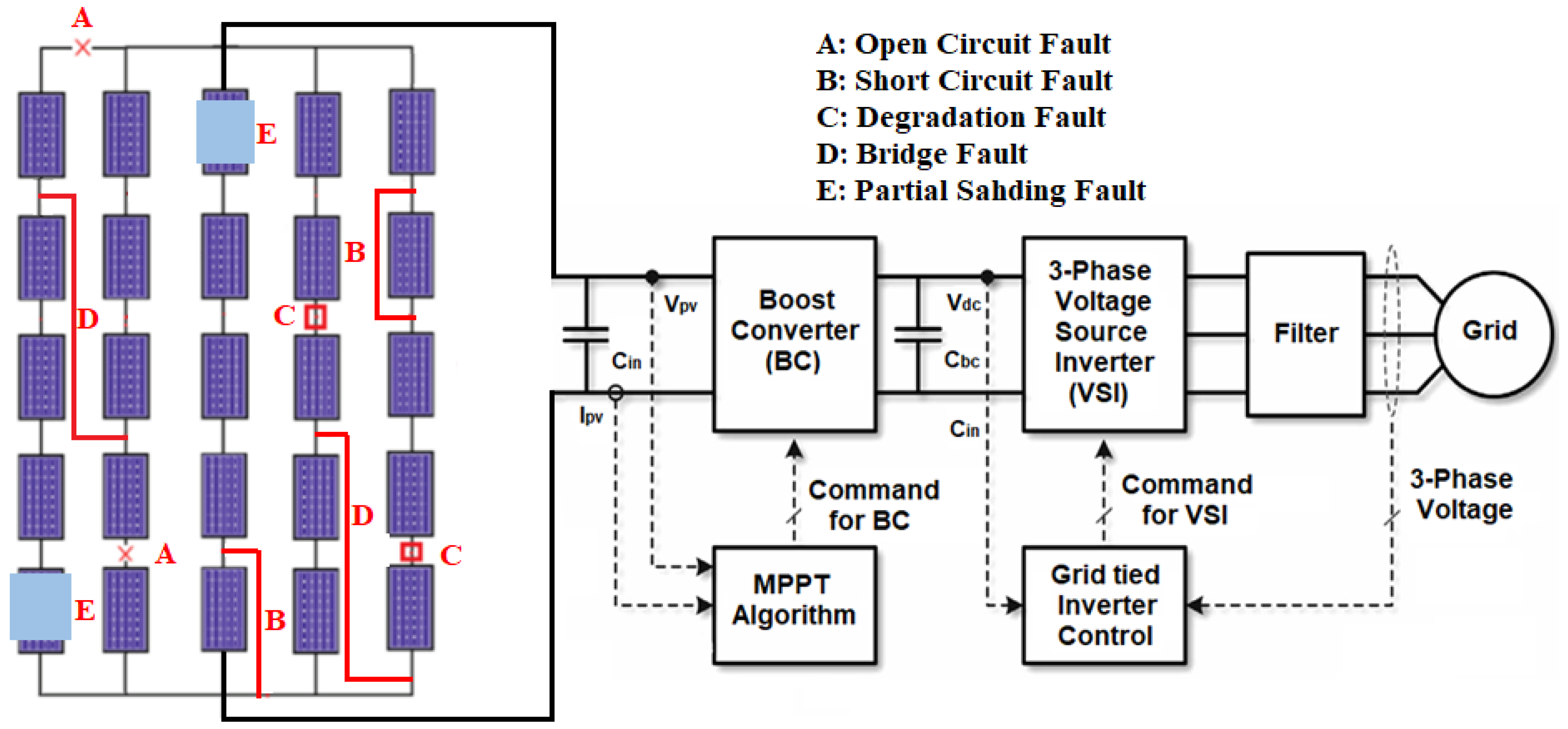
Figure 1. Configuration of grid-connected PV System.
Remotesensing 15 01277 g001
Figure 3. (a) Power–voltage curve under normal scenario. (b) Current–voltage curve under faulty scenario.
Remotesensing 15 01277 g003
Figure 4. Workflow diagram of the proposed fault-diagnosis technique.
Remotesensing 15 01277 g004
Figure 5. Simulink-based model of PV Array System under consideration.
Remotesensing 15 01277 g005
Figure 6. A schematic representation of DNN algorithm.
Remotesensing 15 01277 g006
Figure 7. A schematic representation of LSTM algorithm.
Remotesensing 15 01277 g007
Figure 8. A schematic representation of Bi-LSTM algorithm.
Remotesensing 15 01277 g008
Figure 9. The pseudocode for proposed DSEL fault-diagnosis approach.
Remotesensing 15 01277 g009
Figure 10. Proposed DSEL fault-diagnosis algorithm with base learner models and meta-learner model.
Remotesensing 15 01277 g010
Figure 11. (a) Convergence curves of training accuracy vs. validation accuracy by using DSEL approach. (b) Convergence curves of training loss vs. validation loss by using DSEL approach.
Remotesensing 15 01277 g011
Figure 12. Confusion matrix of different algorithms under noiseless dataset. (a) Proposed DSEL approach. (b) Bi-LSTM. (c) LSTM. (d) PNN. (e) DNN. (f) ANN. (g) Gradient boost. (h) Adaboost. (i) SVM.
Remotesensing 15 01277 g012aRemotesensing 15 01277 g012b
Figure 13. Performance comparison of different algorithms under noiseless dataset.
Remotesensing 15 01277 g013
Figure 14. Radar plot for precision comparison of different algorithms under noiseless dataset.
Remotesensing 15 01277 g014
Figure 15. Confusion matrix of different algorithms under noisy dataset. (a) Proposed DSEL approach. (b) Bi-LSTM. (c) LSTM. (d) PNN. (e) DNN. (f) ANN. (g) Gradient boost. (h) AdaBoost. (i) SVM.
Remotesensing 15 01277 g015aRemotesensing 15 01277 g015b
Figure 16. Performance comparison of different algorithms under noisy dataset.
Remotesensing 15 01277 g016
Figure 17. Radar plot for precision comparison of different algorithms under noisy dataset.
Remotesensing 15 01277 g017
Table 2. Various parameter value combinations for the collection of data.
ParameterTargeted Values
Temperature0 to 60 °C at a step change of 5 °C
Irradiance100 to 1000 W/m2 at a step change of 30
Percentage of Partial Shading30% to 70% at a step change of 15
High Impedances Values25 Ω, 50 Ω, 75 Ω, 100 Ω, 150 Ω, 200 Ω
Fault Impedance0 to 15 Ω at a step change of 5
Table 3. The optimal hyperparameters for the trained base learners and meta-learner.
ModelHyperparatmetersGrid SearchOptimal Parameters
DNNHidden layers{1, 2, 3, 4, 5}2
Learning Rate{0.0001, 0.001, 0.01, 0.1, 0.2}0.001
Input Activation Fuction{“relu”, “sigmoid”, “tanh”, “linear”}Relu
Output Activation Fuction{“relu”, “sigmoid”, “tanh”, “softmax”}Softmax
Optimizer{“SGD”, “rmsprop”, “adagrad”, “adam”}Adam
Epoches{25, 50, 75, 100, 125}125
Batch Size{10, 16, 24, 32, 48}16
Loss Function{ “crossentropy”, “relative entropy”, “sparse categorical crossentropy”}Sparse categorical crossentropy
LSTMHidden layers{1, 2, 3, 4, 5}2
Learning Rate{0.0001, 0.001, 0.01, 0.1, 0.2}0.1
Input Activation Fuction{“relu”, “sigmoid”, “tanh”, “linear”} Relu
Output Activation Fuction{“relu”, “sigmoid”, “tanh”, “softmax”} Softmax
Optimizer{“SGD”, “rmsprop”, “adagrad”, “adam”}Adam
Epoches{25, 50, 75, 100, 125}100
Batch Size{10, 16, 24, 32, 48}32
Dropout{0.3, 0.4, 0.5, 0.6}0.5
Momentum{0.5, 0.6, 0.7, 0.8, 0.9}0.7
Decay rate {0.91, 0.93, 0.95, 0.97}0.95
Loss Function{ “crossentropy”, “relative entropy”, “sparse categorical crossentropy”}Sparse categorical crossentropy
Bi-LSTMHidden Layers{1, 2, 3, 4, 5}1
Learning Rate{0.0001, 0.001, 0.01, 0.1, 0.2}0.0001
Bi-LSTM Nodes{10, 15, 20, 25, 30}30
Input Activation Fuction{“relu”, “sigmoid”, “tanh”, “linear”} Relu
Output Activation Fuction{“relu”, “sigmoid”, “tanh”, “softmax”} Softmax
Optimizer{“SGD”, “rmsprop”, “adagrad”, “adam”}Adam
Epoches{25, 50, 75, 100, 125}75
Batch Size{10, 16, 24, 32, 48}32
Dropout{0.3, 0.4, 0.5, 0.6}0.4
Momentum{0.5, 0.6, 0.7, 0.8, 0.9}0.6
Decay rate {0.91, 0.93, 0.95, 0.97}0.97
Loss Function{ “crossentropy”, “relative entropy”, “sparse categorical crossentropy”}Sparse categorical crossentropy
MLRSolver{“newton-cg”, “sag”, “saga”, and “lbfgs”}lbfgs
Iterations{20, 50, 80, 100, 130}100
Penalty{“l1”, “l2”, “elasticnet”, None}l2
C-value [0.001, 0.01, 0.1, 1, 10]1
Table 4. Comparative analysis of different fault-diagnosis algorithms under noiseless dataset.
AlgorithmsAccuracyPrecisionSensitivityF1-Score
DSEL Algorithm98.62%98.52%98.66%98.50%
BI-LSTM95.66%95.83%95.66%95.61%
LSTM93.35%94.01%93.33%93.21%
PNN92.11%92.63%92.33%92.04%
DNN 91.89%91.97%92.01%91.89%
ANN 90.37%90.16%89.98%89.83%
Gradient Boost 87.83%87.83%87.83%87.16%
AdaBoost85.26%86.88%85.29%84.83%
SVM82. 75%82.66%82.83%82.33%
Table 5. Comparative analysis of Different fault-diagnosis algorithms under noisy dataset.
AlgorithmsAccuracyPrecisionSensitivityF1-Score
DSEL Algorithm94.87%95.10%94.87%95.06%
BI-LSTM89.18%90.11%89.33%89.33%
LSTM86.15%89.08%86.16%85.57%
PNN86.53%87.03%86.53%86.72%
DNN85.88%86.50%85.83%85.89%
ANN84.98%86.16%85.88%86.17%
Gradient Boost82.58%82.19%82.94%82.16%
AdaBoost80.84%81.68%80.81%80.66%
SVM74.87%76.95%74.86%72.50%
Disclaimer/Publisher’s Note: The statements, opinions and data contained in all publications are solely those of the individual author(s) and contributor(s) and not of MDPI and/or the editor(s). MDPI and/or the editor(s) disclaim responsibility for any injury to people or property resulting from any ideas, methods, instructions or products referred to in the content.