Abstract
Semantic segmentation of high-resolution remote sensing images plays an important role in many practical applications, including precision agriculture and natural disaster assessment. With the emergence of a large number of studies on convolutional neural networks, the performance of the semantic segmentation model of remote sensing images has been dramatically promoted. However, many deep convolutional network models do not fully refine the segmentation result maps, and, in addition, the contextual dependencies of the semantic feature map have not been adequately exploited. This article proposes a hierarchical refinement residual network (HRRNet) to address these issues. The HRRNet mainly consists of ResNet50 as the backbone, attention blocks, and decoders. The attention block consists of a channel attention module (CAM) and a pooling residual attention module (PRAM) and residual structures. Specifically, the feature map output by the four blocks of Resnet50 is passed through the attention block to fully explore the contextual dependencies of the position and channel of the semantic feature map, and, then, the feature maps of each branch are fused step by step to realize the refinement of the feature maps, thereby improving the segmentation performance of the proposed HRRNet. Experiments show that the proposed HRRNet improves segmentation result maps compared with various state-of-the-art networks on Vaihingen and Potsdam datasets.
1. Introduction
In recent years, semantic segmentation models for high-resolution remote sensing images have emerged in an endless stream, which has also promoted the development of many applications, including precision agriculture, natural disaster assessment, and urban planning [1,2,3,4,5]. Many traditional semantic segmentation methods have also achieved good results, but with the development of deep learning, because the semantic segmentation model of deep learning has stronger timeliness, it is more applicable to actual situations. As the pioneering work of semantic segmentation, a fully convolutional network (FCN) [6] has opened up a new path for image segmentation. Next to the encoding and decoding structures, multi-scale feature extraction blocks and attention-based blocks in semantic segmentation models appear to improve model performance, but each structure has its advantages and disadvantages, and some models even use them in combination to boost the performance of the semantic segmentation model of remote sensing image.
Since the emergence of the FCN model, it was better than the traditional image segmentation method [7,8] in terms of segmentation accuracy and time consumption. FCN has achieved good results, but because many convolution operations are used to extract features, much primary feature information is lost. So, the skip connection method is used to achieve feature compensation. Models of encoding and decoding structures have also gradually emerged. Encoding means that the resolution of feature maps is gradually reduced, while extracting features with convolution and pooling operations, and decoding means that the resolution of feature maps is gradually increased through upsampling operations. In the end, the model obtains input and output images of the same size. At present, there is still a lot of research [9,10,11] using the structure of encoding and decoding. The advantage of this structure is that it can alleviate the problem of loss of feature map information. For instance, UNet [12] was a classic encoding and decoding structure model, and it used skip connections to achieve fusion before and after feature extraction to make up for the lack of important features. DeconvNet [13] used VGGNet [14] to delete the fully connected layer as a feature extractor based on an encoding and decoding structure, but the model employed deconvolution operations in the decoding stage to restore the resolution of the feature map, which alleviated the problem of missing features. In addition, the model complexity increased a lot. LinkNet [15] also adopted the encoding and decoding structure to meet the real-time requirements of semantic segmentation and reduced the amount of model parameters and time consumption of the model by increasing the stride of the convolution operation.
The multi-scale feature extraction block has been widely used in the semantic segmentation model because this module has a strong role in mining the continuous context information, and it aims to enhance the ability of the model in recognizing objects of different scales in the image. DeepLabV3+ [16] used dilated convolution to achieve feature extraction at different scales, and PSPNet [17] used parallel pooling at different scales to extract key features of different types of ground objects so as to increase the segmentation performance of the model. DFCNet [18] adopted multi-scale convolution operations to widen the model and advance the variety and abundance of extracted features, and it also adopted the fusion of multi-modal data to refine the segmentation result map. Hoin et al. [19] proposed a model that uses features from different decoding stages to enhance the features of the holistically nested edge detection unit, and it finally achieved feature fusion at different scales to enhance the generalization ability of the model. MSA-UNet [20] combined the multi-scale feature extraction module with the Unet model, and it utilized the feature pyramid module to realize the refinement of object edges. The sub-modules of RCCT-ASPPNet [21] were dual decoding structures and atrous spatial pyramid pooling (ASPP), which cross-fused global and local semantic features of different scales, thus further promoting the model segmentation performance.
The attention mechanism module is derived from the study of human vision and aims to focus more on key areas in the image than other areas. In the field of computer vision, the purpose of the attention mechanism module is to enhance the weight of salient features and reduce the weight of noise and useless information in the image so as to achieve the purpose of extracting salient features in the image. Recently, many studies [22,23,24,25] have been proposed based on the attention mechanism. For instance, SE-Block [26] was a classic attention mechanism method. Its motivation was to explicitly establish the interdependence relationship between feature channels. Specifically, it was to automatically obtain the weight of each channel through model learning and then according to this weight, promote useful features, and suppress useless features for the current task. CBAM-Block [27] was an attention mechanism module that combined spatial and channel information. Compared with SE-Block, which only focused on the channel attention mechanism, it achieved better performance. MCAFNet [28] extracted features through the feature extractor, and the global–local transformer block mined the context dependencies in the image, and the channel optimization attention module mined the context dependencies between feature map channels, thereby increasing the expressiveness of features. Zhang et al. [29] proposed a model whose submodule, the semantic attention (SEA), consisted of a fully convolutional network, and this module enhanced the stimulation of regions of interest in the feature map and suppressed useless information and noise in the feature map. In addition, the scale complementary mask branch (SCMB) module realized feature extraction at different scales and made full use of multi-scale features. The two sub-modules were multiscale attention (MSA) and nonlocal filter (NLF) in MsanlfNet [30], and the former enhanced the expressive ability of features by using the multi-scale feature attention module, and the latter captured the dependence of global context information, and the model improved performance through these modules.
In summary, the model of encoding and decoding structure, multi-scale feature extraction block, and attention mechanism block, have significantly improved the accuracy of semantic segmentation of remote sensing images, but these models are not obvious for feature map refinement operations. In addition, mining the contextual dependencies of the position information and channel information in the feature map is not thorough. Therefore, in the proposed hierarchical refinement residual network (HRRNet), the channel attention module (CAM) and pooling residual attention module (PRAM) are put forward to fully exploit the contextual dependencies of the feature map position information and channels, thus enhancing the deep expressive ability of features. The fusion of features realizes the refinement of feature maps. In addition, the attention block, the pooling residual structure in PRAM, and the residual structure between CAM and PRAM modules can significantly promote the performance of the network.
The main contributions of the proposed HRRNet are summarized as follows:
- (1)
- The proposed CAM and PRAM sub-modules of HRRNet can fully exploit the feature map position information or the dependence of the context information between channels to enhance the deep expressive ability of features.
- (2)
- Using ResNet50 as a feature extractor, the layered fusion of features extracted to different stages and different scales realizes the refinement of the feature map, and the fusion of multi-scale features also enhances the model’s ability to recognize various types of ground objects and promotes the generalization ability of the model.
- (3)
- By setting different residual structures, the correlation between gradient and loss in the model training process is improved, which enhances the learning ability of the network and alleviates the problem of gradient disappearance.
2. Related Work
2.1. Semantic Segmentation Model with Attention Mechanism
Since it is very important to highlight details in complex scene images, modules that simulate human attention mechanisms are used in various fields. Attention-based methods have emerged in a large number of studies [31,32,33,34] in recent years.
The attention mechanism has also achieved good results in semantic segmentation tasks. SEBlock [26] was to explicitly establish the interdependence relationship between feature channels. Compared with SE-Block, SKNet [35] performed convolution kernel operations of different sizes on the same input, enabling neurons to collect and fuse multi-scale features at the same stage, and it further explored the dependencies between spaces and channels. SERNet [36] integrated SE-Block and residual structure, thus mining long-range dependencies in the spatial and channel dimensions in the feature map. RSANet [37] improved the self-attention mechanism module, and its sub-modules may mine the relationship between pixels in salient regions, which was more logical for grasping the context information of the image. Through two parallel branches, DANet [38] passed the features extracted by the feature extractor through the channel attention module and the position attention block, respectively, and it further mined the information of key features in the feature map. The contextual transformer (CoT) block in CoTNet [39] cross-fused features extracted by convolution kernels of different scales, and this module increased the continuity of contextual information in the feature map. LANet [40] used the fusion of advanced features and low-level features to complement semantic information and geometric information, and it used an average pooling operation and residual structure in the sub-module to enhance the expressive ability of features. However, in high-resolution remote sensing images, it seemed that one-time pooling could not fully extract salient features. Therefore, SPANet [41] used successive pooling operations to extract more salient features. The improved model has better segmentation results for small-scale targets and object edges.
2.2. Semantic Segmentation Model Based on Multi-Branch Feature Fusion
In many studies [42,43,44], features are extracted through feature extractors, and then features are enhanced at different stages, and finally features of different scales are fused to increase the model’s ability to recognize objects of different scales and enhance the robustness of the model. Usually, ResNet50 [45], HRNet [46], and the Inception [47] Network are often used as feature extractors. The features extracted at different stages have different characteristics. The features extracted in the shallow model contain edge texture and geometric information, and the deep features contain advanced semantic features, so the method of multi-stage feature fusion can alleviate the problem of information loss in the semantic segmentation model. Specifically, MANet [48] used ResNet 50 as a feature extractor and enhanced the extracted features to the four stages and then fused them step by step to increase the segmentation accuracy of the model. Its sub-modules fully mined the dependence on the context information of the feature map and explored the relationship between pixels, which played a key role in improving the performance of the model. Zuo et al. [49] proposed a MDANet in which a deformable attention module (DAM) integrated a sparse spatial sampling strategy and context information dependencies to capture the structural information of each adjacent pixel in the feature map. Besides, the low-level features in the shallow network in the AFNet [50] model contained small-scale target location information, and the high-level features in the deep network contained feature information of large-scale targets. These features enhanced the expressive ability of features through the scale-feature attention module (SFAM). CF-Net [51] used the backbone to obtain accurate multi-scale semantic information from the image, and it utilized the cross-fusion block to broaden the receptive field of the model, especially for the segmentation accuracy of small-scale objects, which has been greatly improved. Zhao et al. [52] proposed a model that integrated pyramid attention pooling blocks and attention mechanism blocks to implement a multi-scale module for adaptive feature refinement. In order to extract more detailed features, the pooling index correction module was employed to restore fine-grained features.
2.3. Semantic Segmentation Model Based on Transformer
Recently, transformer-based models have also been applied to semantic segmentation tasks and have achieved good results. For instance, WiCoNet [53] employed traditional convolution operations to extract features and aggregated information in local areas of images through another sub-module. Moreover, the model introduced a context transformer to embed contextual information and selectively projected it onto the local features, thus achieving better results. Song et al. [54] proposed a convolutional neural network (CNN) and transformer multiscale fusion network, which combined the CNN and transformer to enhance the segmentation performance of the model. Specifically, the CNN had a strong ability to represent hierarchical feature information, and the transformer had the potential in mining the dependence of global context information, and, in addition, the sub-modules of the network fused the context information of local and global features to enhance the expressive ability of features. More recently, Zhang et al. [55] proposed a transformer and CNN hybrid deep neural network. This model used the swin transformer to extract features and achieve better long-range spatial dependencies. In addition, an atrous spatial pyramid pooling block based on depthwise separable convolution (SASPP) was applied to obtain the features of different scales context. This model greatly improved the accuracy of remote sensing image edge semantic segmentation. Likewise, He et al. [56] proposed a model that embedded the swin transformer into the classic UNet model to construct a new double decoding structure. This model established pixel-level correlation to encode the spatial information in the swin transform, thus enhancing the feature expression ability of the network. In addition, the model compressed the features of small-scale objects to improve the segmentation accuracy.
3. Proposed Network Model
The flowchart of HRRNet is shown in Figure 1. HRRNet consists of a backbone (feature extraction stage), four attention blocks, and five decoders. In this study, ResNet50 is used as a feature extractor, also known as backbone. An attention block is composed of CAM, PRAM, and residual structures, which play the roles of enhancing feature expression ability and aim to mine context dependencies in feature maps. A decoder consists of convolution, activation function, and deconvolution operation, and its function is to change the channel of the feature map and perform upsampling operations. The convolution operation is defined as:
where stands for the dimensions of the output feature map, represents the dimensions of the input feature map, k is the size of the convolution kernel, s stands for stride during the convolution operation, represents adding a few pixels to the edge of the feature map matrix, and stands for the padding of the output feature matrix. Specifically, the input of HRRNet is an image with a size of 3 channels × 256 × 256, and ResNet50 is used as the backbone to extract features, and the features of the four stages are, respectively, defined as , , and , and their number of channels and sizes are 256 channels and 64 × 64, 512 channels and 32 × 32, 1024 channels and 16 × 16, 2048 channels and 8 × 8, respectively. Then, is fed to the attention block (AB), the output feature matrix is defined as , and then is input to Decoder4, the number of channels and the size of the output feature matrix are 1024 channels and 16 × 16, the output is defined as , and then the corresponding elements of and S3 feature map are calculated by the sum operation to realize the fusion of feature maps, which is defined as the feature matrix :
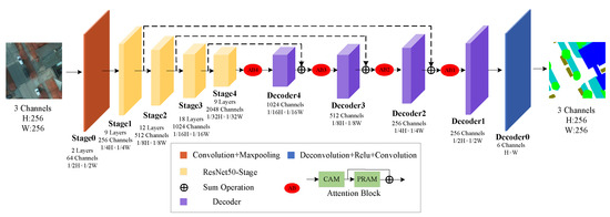
Figure 1.
Flowchart of the proposed HRRNet.
Then, is fed to CAM and PRAM, and the output feature map matrices are and , respectively. The attention matrix of the output Attention Block is defined as :
3.1. Illustration of the Proposed HRRNet
In addition, , and also achieve feature fusion with the previous stage in this way to complete the refinement of the feature matrix and finally output 3 channels and 256 × 256. HRRNet network training details are shown in Algorithm 1.
| Algorithm 1 Train an optimal HRRNet model. |
Input: Input a set of images and their labels . Output: Get the segmentation results of the test set.
|
3.2. Channel Attention Module
Figure 2 shows the channel attention module (CAM) of the proposed HRRNet. Assume that M and C represent the dimension of the input feature matrix and the number of channels, respectively, where , , and represent the height and weight of the input feature matrix, respectively. Assume that we input a feature matrix . CAM generates the corresponding feature matrices Q, K, and V by operating on different branch feature matrices as:
where , and represent the operation on the feature map F in different branches. It is worth noting that the reshape operation performed on the feature map matrix F in each stage of the CAM process is represented by , , and . T represents the transpose of the feature map, and I represents the dimension of the transformed feature map channel. Because the Q, K, and V feature maps have the same channel dimensions, we use the same expression.
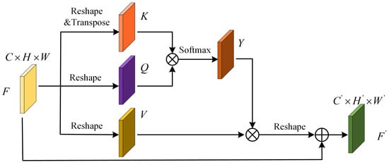
Figure 2.
Flowchart of the proposed CAM.
The feature matrix K and Q are multiplied by elements between channels, the symbol ⊗ represents channel element-level multiplication operation, and the similarity between the feature matrices is calculated through this operation. The result of an activation function usually represents the similarity between feature maps, the feature maps output by the operation is defined as Y, and the similarity between channels is calculated by the activation function is expressed by weight:
where represents the activation function :
Here, Y represents the similarity matrix between the feature matrix K and Q, corresponding to the channel. Next, the output of the product operation of Y and the feature matrix V is defined as the feature matrix , which is reshaped to have the same channel number and size as the input feature map F. Finally, the summation operation is performed to output the result :
It is worth noting that the input and output of CAM are feature maps of the same dimension and same size. Through a series of operations of this module, the contextual dependencies between feature map channels are fully excavated, and the representation ability of salient features is enhanced.
3.3. Pooling Residual Attention Module
Figure 3 shows the PRAM of the proposed HRRNet. Assume that and represent the dimension of the input feature matrix and the number of channels, respectively, where , and represent the height and weight of the input feature matrix, respectively. The feature matrix is output from the CAM module. PRAM implements 1 × 1 convolution operation on different branch feature matrices to generate corresponding feature matrices and :
where represents the 1 × 1 convolution operation performed on the feature map matrix to generate the feature map matrix, represents the 1 × 1 convolution operation performed on the feature map matrix to generate the feature map matrix, represents the operation of the feature map, T is defined as the transpose of the feature matrix, and is defined as the channel dimension of the transformed feature matrix. Because the and feature matrix channel dimensions are the same, we use the same expression.
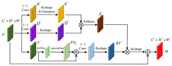
Figure 3.
Flowchart of the proposed PRAM.
The feature matrices and are multiplied by elements between channels, and, after the output is passed through the activation function , the final output feature matrix Z is obtained. Then, the activation function is used to calculate the similarity of the feature map position:
Next is the operation of the third branch of the feature matrix . Here, and are the length and width of the feature map . Specifically, the average pooling operation is first performed on the feature map , and the resulting feature map is defined as P. At this time, the corresponding relationship between the original feature map and the pooling feature map is defined as:
where is the value of each element of the feature map after average pooling, , is the cth channel of the feature map. By performing the bilinear interpolation, the feature map is upsampling to obtain . The purpose is to perform the summation between the corresponding channels with the feature map to obtain the feature map . Next, we perform a 1 × 1 convolution operation on and the operation, which is defined as:
Finally, the and Z feature maps are multiplied between corresponding elements, and the feature map is summed to output the feature map M:
4. Experiments and Results
4.1. Dataset
The model uses two datasets of ISPRS Vaihingen and Potsdam to verify its validity. The first one is the Vaihingen dataset. It is composed of 33 tiles with an average size of 2500 × 2100, and the ground resolution is 9 cm. Tile consists of red, green, blue, and infrared (RGB-IR) four-channel, and a digital surface model (DSM) is provided in this Vaihingen dataset. This ground truth has six categories, including: buildings, impervious surfaces, low vegetation, tree, clutter, and car. For assessment, the 17 ground truth images are classified into three groups, 11 images are used as the training set, two images are used for the verification set, and four pictures are used for the test set.
The second one is the Potsdam dataset. It is composed of 38 tiles with an average size of 6000 × 6000, and the ground resolution is 5 cm. Tiles are RGB-IR images with four channels. The Potsdam dataset also has a DSM. The ground truth of the Potsdam dataset has the same number of categories as that of the Vaihingen dataset. For assessment, the 24 ground truth images are classified into three groups, 19 images are used as the training set, two images are used for the verification set, and three images are used for the test set.
4.2. Dataset Preprocessing and Evaluation Metrics
In high-resolution remote sensing images, the distribution of multiple categories of ground objects is chaotic, so the labeling of dataset labels is very difficult, which leads to a small amount of annotated datasets. Therefore, the training sets of Vaihingen and Potsdam use random flipping and mirroring for data enhancement to achieve the purpose of expanding the amount of data. We employed test time augmentation (TTA) in the flipping and mirroring stages of the image. In this study, the albumations library was adopted to implement Vaihingen and Potsdam data augmentation. After augmentation, the images of the training sets were normalized to [0, 1]. It is worth noting that other models also use the same data augmentation operation.
The performance of those models on the Vaihingen and Potsdam datasets is verified by the mean intersection over union (), the overall accuracy (), the F1 score () and the mean F1 score () indicators, which are calculated based on the confusion matrix as follows.
4.3. Training Details
Before model training started, the learning rate was set as , and it was reduced to 0.85 times after every 15 epochs. In addition, we used Adam as the optimizer for the training model, and the polynomial learning rate was set as (1 − (cur_iter/max_iter)), the learnable parameters’ weight attenuation was set as , and the number of maximum iterations was set as . In this study, the model utilized the following loss function by combining the cross-entropy function and median frequency balancing weights.
where is the weight for class a, is the pixel frequency of class a, is the probability of sample belonging to class a, and denotes the class label of sample n in class a. For the Vaihingen and Potsdam datasets, the training sets are cropped and augmented to 5000 images of size 256 × 256, and the batch size is set to 5. We employed a sliding window (with a size of 448 × 448 and a step size of 100 pixels) on the test set by averaging the predicted results of the overlapping patches as the final results.
4.4. Ablation Study
The proposed submodule attention block of HRRNet fully explored contextual dependencies, and the enhanced features of multiple branches are fused step by step to refine the segmentation results. In order to prove the effectiveness of the attention block, CAM and PRAM on the experimental results, we made different experimental settings. First, we added an attention block on different branches based on the backbone (ResNet50). It was worth noting that adding an attention block each time was based on the previous model. Regardless of whether there was an attention block on each branch, multiple stages of feature fusion were performed step by step. Second, the attention block in the four branches remained unchanged, and the CAM, PRAM, and residual structures were sequentially added to obtain experimental results to prove their efficiency.
The results of two groups of ablation experiments on the Vaihingen dataset are shown in Table 1 and Table 2. Table 1 shows the ablation results of the first set on the Vihingen dataset. It is clear that and increased by 2.84% and 5.23% after adding an attention block on the basis of Backbone, especially , which increased by 7.87%. It shows that the attention block has greatly improved the performance of the model. In addition, with the increase of the attention block, all the indicators have been promoted, which proves that the attention block can fully explore the contextual dependencies of positions and channels. Finally, the experimental results are optimal when we add the attention block to each branch. Table 2 shows the results of the second set of ablation experiments. At this time, we kept the number of attention blocks unchanged, and the CAM, PRAM, and residual structures were added to the attention block in order. It is shown from Table 2 that , , and increased by 2.95%, 5.19%, and 7.80%, respectively, after adding CAM, which proves that the CAM module fully exploits the contextual dependencies between feature map channels, thus increasing the segmentation of the model performance. Immediately after the PRAM module was added to the attention block, the contextual dependencies of the feature map position can be fully exploited, and , , and increased by 0.21%, 0.41%, and 0.62%, respectively, indicating that the pooling residual structure increases the feature expressive ability. Finally, adding the residual structure to the attention block is HRRNet, especially mIou, which increased by 0.54%, which proves the effectiveness of the residual structure.

Table 1.
Ablation results of the first set (on Vaihingen data set), the optimal results are bolded.
Table 2.
Ablation results of the second set (on Vaihingen data set), the optimal results are bolded.
The results of two sets of ablation experiments on the Potsdam dataset are shown in Table 3 and Table 4. Table 3 shows the results of the first set of ablation experiments. The experimental results show the same trend as the indicators on the Vaihingen dataset. With the increase in the number of attention blocks, the performance of the model gradually reaches the optimum. Table 4 shows the results of the second group of ablation experiments. It is worth noting that, after adding PRAM, , , and increased by 1.83%, 1.55%, and 2.64%, respectively, which fully proves that the contextual dependencies of the position can be further exploited to advance the segmentation performance of the HRRNet.All in all, the ablation experimental results on the Vaihingen and Potsdam datasets show the same trend, which proves the robustness of the HRRNet model, and it also shows that CAM and PRAM can fully mine the contextual dependencies of the channel and position in the feature map. In addition, the attention block of multiple branches realizes the purpose of refinement of the feature map.
Table 3.
Ablation results of the first set (on Potsdam data set), the optimal results are bolded.
Table 4.
Ablation results of the second set (on Potsdam data set), the optimal results are bolded.
4.5. Quantitative Comparison of Different Models
In order to further verify the efficiency of the proposed HRRNet, we also reproduced the classic semantic segmentation models and compared them with the HRRNet. First of all, methods based on attention mechanism, including CBAM-Block [27], SE-Block [26], SK-Block [35], DANet [38], and CoTNet [39], all of which have a common feature, that is, to enhance the expressive ability of features through modules, so that salient features can be extract. In addition, semantic segmentation models based on multi-scale feature extraction, including DeepLabV3+ [16] and PSPNet [17], these models used dilated convolution or multi-scale pooling to extract features at different scales to grasp the dependencies of contextual information in images. However, they improved model performance by increasing the complexity of the model. In addition, peer models designed for semantic segmentation remote sensing images, such as LANet [40] and SPANet [41], were also chosen for comparison. For the fairness of experimental results, all models use ResNet50 as a feature extractor.
Table 5 shows the experimental results of various models on the Vaihingen dataset. It shows that the experimental results based on the attention mechanism model are slightly better than the multi-scale model. The , , and of the SK-Block model are 1.87%, 3.22%, and 4.93% higher than those of PSPNet. The purpose of the attention mechanism module is to increase the weight of salient features in the feature map and suppress noise and useless information, and the multi-scale feature extraction model increases the complexity of the model and improves the continuity of context information, but the attention mechanism module obtains better experimental results. In addition, the , , and of the CoTNet model are 2.02%, 3.07%, and 4.68% higher than those of DeepLabV3+. For LANet and SPANet models, what they have in common is the fusion of advanced semantic features and shallow features to complement geometric information and spatial information, but their difference is the feature enhancement module. LANet employed a pool to enhance the representation of features ability, while SPANet employed a successive pooling strategy to extract key salient features, and the segmentation of target boundaries was more accurate. However, HRRNet makes up for the shortcomings of the above models and adopts the fusion of features of different scales at different stages to realize the refinement of feature maps.
Table 5.
Experimental results for various models (on Vaihingen data), the optimal results are bolded.
Table 6 shows the experimental results of various models on the Potsdam dataset. The experimental results of the model based on the attention mechanism are better than those of the multi-scale feature extraction model. This trend is similar to the experimental results on the Vaihingen dataset. DANet performed very well on the Potsdam dataset, and the position attention module and channel attention module played a big role in the performance of the model. CoTNet promoted the performance of the model by further exploring the contextual dependencies in the feature map through the convolution operation of multiple branches and adding the sum product operation between the feature maps. Table 6 shows that the , , and of the DANet model are 2.51%, 1.69%, and 2.78% higher than those of CoTNet, but the performance of the DANet model needs to be improved. SPANet used a successive pooling strategy to improve model performance. The , , and of the SPANet model are 0.26%, 0.49%, and 0.88% higher than those of DANet. HRRNet explores the contextual dependencies between positions and channels and uses multi-stage feature map fusion to implement refinement operations to further improve the segmentation performance of the model. The , , and of the HRRNet model are 0.97%, 0.53%, and 0.9% higher than SPANet. In addition, the of the surface, building, and Low-veg categories are 1.14%, 0.98%, and 0.86% higher than SPANet.
Table 6.
Experimental results for various models (on Potsdam data), the optimal results are bolded.
For the experimental results, the , , and of the HRRNet model are 0.98%, 1.71%, and 2.69% higher than those of LANet, and 0.58%, 0.93%, and 1.46% higher than those of SPANet, and the of Low-veg, tree, and car categories are 1.62%, 0.74%, and 1.86% higher than those SPANet. The HRRNet model can obtain better segmentation performance.
All in all, the experimental results of HRRNet compared with various models on these two datasets show that the HRRNet has strong robustness and good segmentation performance.
5. Discussion
The complexity of the model is also an important indicator for judging the performance of a model. We also compared the parameter amount, floating-point operations (FLOPs), and inference time of HRRNet and other models. The larger the model, the larger the amount of memory occupied and the lower the real-time performance, but the segmentation accuracy is still very important. Table 7 shows the indicators of different models. In order to maintain fairness, the input of all models is 3 × 256 × 256. It can be seen from Table 7 that multi-scale feature extraction models, such as PSPNet and DeepLabV3+ models, have the largest number of parameters, and the PSPNet model has the highest FLOPs, but their segmentation results are not ideal. LANet and SPANet are dual-branch feature fusion strategies, with slightly lower parameters and FLOPs, but HRRNet adopts a strategy of step-by-step fusion of four-branch feature maps to refine feature maps, which improves the segmentation performance at the cost of a small number of model complexity. Additionally, we compared the inference time of all competing models on CPU and GPU, which was also one important indicator of model complexity. The implemented GPU is NVIDIA Geforce GTX 2080Ti, and the model of the CPU is Intel (R) Xeon (R) Silver 4210. It is observed that HRRNet sacrifices a small amount of inference time to accomplish higher segmentation performance.
Table 7.
Complexity metrics for various models. (The input is the 3 × 256 × 256).
5.1. Qualitative Analysis of the Segmentation Results from Ablation Experiments
Quantitative analysis can objectively explain the performance of the model, and the segmentation maps can more subjectively explain the segmentation performance of the model. In this subsection, we illustrate the function of the proposed main submodules and structures by presenting segmentation maps of ablation experiment results. Figure 4 shows the segmentation results of the model on the two data sets after adding the attention block in order on the basis of the backbone. Figure 4a,b are the selected results on the Vaihingen dataset. It can be seen from Figure 4a that, with the addition of the attention block, the Low-veg category is wrongly segmented until the final segmentation result basically matches the label. It can be seen from Figure 4b that the segmentation map of the building category is also gradually more precise, and we know that the attention block is accompanied by the addition of different branches to improve the expressive ability of the features so that it is constantly refining the segmentation map. It plays a great role in improving the performance of the model. The segmentation maps show that it is consistent with the experimental data in Table 2 and Table 4.
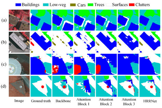
Figure 4.
On the basis of backbone, the segmentation result map after adding the attention block in sequence. Rows (a,b) are the selected results on the Vaihingen dataset. Rows (c,d) are the selected results on the Potsdam dataset.
Figure 5 shows the segmentation results of the model on the two data sets after adding CAM, PRAM, and residual structure in order based on the backbone. Figure 5a,b are the selected results on the Vaihingen dataset. It is obvious that, with the addition of CAM and PRAM, the accuracy of the segmentation map of the building category is improving step by step until all modules and structures are added. Although the final segmentation map still has some defects, it is already very close to the label. The category of Low-veg in Figure 5b is more likely to be misclassified, but there has been a significant improvement in the segmentation map of HRRNet. Figure 5c,d are the selected results on the Potsdam dataset. The objects in these original images all have a characteristic of whether they have specific outlines, so the segmentation results can reflect whether the model has good segmentation performance, especially after adding CAM and PRAM, and the segmentation results have been significantly improved. The wrongly segmented areas are also reduced, indicating that the CAM and PRAM modules play a key role in excavating the contextual dependencies between channels or feature maps. In the end, the segmentation results of HRRNet are closer to the labels and the proposed HRRNet achieves the refinement of the segmentation results.
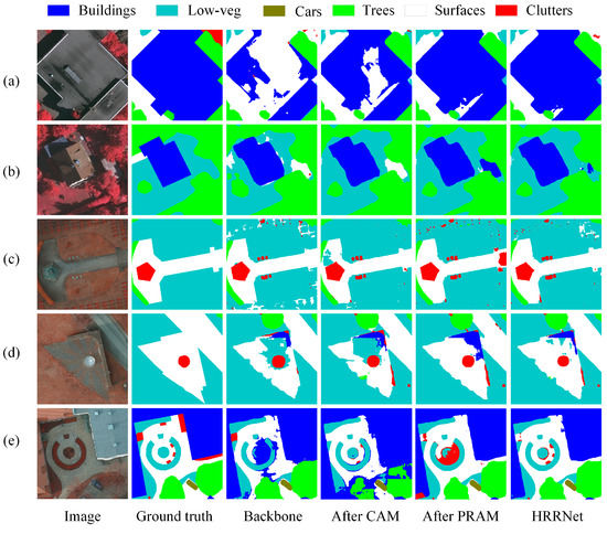
Figure 5.
On the basis of backbone, the segmentation result map after adding the CAM and PRAM in sequence. Rows (a,b) are the selected results on the Vaihingen dataset. Rows (c–e) are the selected results on the Potsdam dataset.
5.2. Qualitative Analysis of the Segmentation Results from Various Models
In this subsection, we fully verify the superiority of HRRNet performance by analyzing the segmentation results of various models. Figure 6 shows the results cropped on the Vaihingen and Potsdam test datasets, and the details of the segmentation are easier to show clearly. Figure 6a mainly shows the segmentation of car categories by various models. In high-resolution remote sensing images, car categories belong to the segmentation of small objects, which is very difficult for models to accurately segment. It can be seen that the DeepLabV3+ of multi-scale feature extraction is very vague for the segmentation of the car boundary, and there are misclassified areas on the edge of the car category. From the segmentation prediction maps of the SPANet, it has been proved that the accuracy of each car category segmentation has been improved. However, from the segmentation prediction maps of the HRRNet, it can be clearly seen that the edge details of the adjacent vehicle categories can also be segmented, and the result is very accurate. Figure 6b shows the segmentation results of various models for buildings and Low-veg categories. Except for the precise segmentation of HRRNet, other models misclassify the Low-veg category into the surfaces category in the same area, which validates that the HRRNet has more efficient performance compared to other various models. Figure 6c,d are the selected results on the Potsdam dataset. (c) shows the segmentation of buildings and Low-veg categories. From the segmentation results, it can be seen that DeepLabV3+ and SKNet have misclassified some areas of building categories, but LANet and CoTNet have accurately segmented the building categories. However, CoTNet also suffers from segmentation errors in the surfaces category. The segmentation results of SPANet are better than other models, but the HRRNet model is more accurate at the edges. The objects in Figure 6d are similar to the building categories, DeepLabV3+ is wrongly segmented, and the segmentation results of other models are gradually becoming more accurate. However, the result of HRRNet segmentation is the best, especially for the segmentation of a cluttered area, which is not correctly segmented by other models.
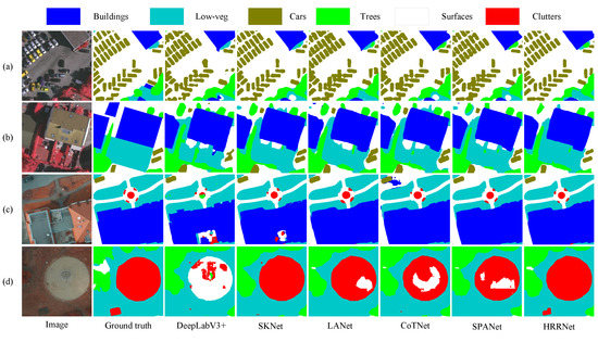
Figure 6.
Visual segmentation maps for various models. Rows (a,b) are the results of cropping on the Vaihingen dataset. Rows (c,d) are the results of cropping on the Potsdam dataset.
Figure 7 shows the high-resolution segmentation results of various models cropped on the Potsdam dataset. It could be obtained from the original image that the scene is complex and diverse, and it is difficult to segment different types of ground objects. The DeepLabV3+ cannot accurately segment the building category. SKNet is misclassified as the building category when segmenting the surfaces category. LANet, CoTNet, and SPANet appear ambiguous when segmenting the edge of the building, although the segmentation results and labels of some areas of HRRNet are inconsistent, HRRNet still segments more precise areas than other models. It is noteworthy that, in order to compare the segmentation performance of each model, some areas in the segmentation maps of each model are marked with red boxes.
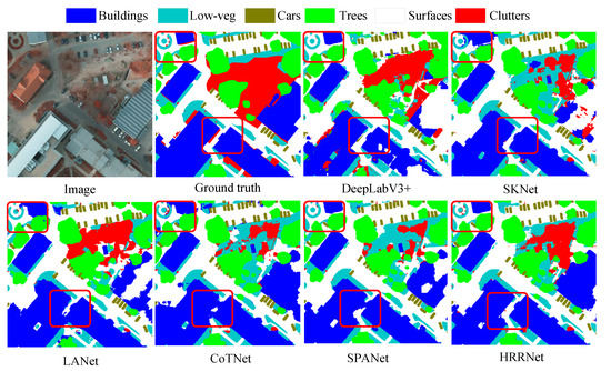
Figure 7.
Visual segmentation maps for various models. These maps were the selected results on the Potsdam dataset.
In summary, from the segmentation results of various models in Figure 6 and Figure 7, it can be concluded that HRRNet makes up for the shortcomings in other models. Specifically, Peer models, such as LANet and SPANet, use a dual-branch feature fusion strategy so that they do not fully utilize the features extracted by the feature extractor (ResNet50). In addition, they use 4 times or 8 times upsampling strategy to expand the size of the feature map, but the loss of detailed information in the feature map is particularly significant, thus reducing the segmentation performance of the model. Compared with the proposed HRRNet model, the features of different stages extracted by the feature extractor (ResNet50) are fully utilized, and the contextual dependencies of channels and positions in the feature map are explored through CAM and PRAM to enhance the expressive ability of features. In addition, HRRNet performs the process of feature fusion of each branch, and it uses the deconvolution strategy to perform only 2 times upsampling operations, which not only fully utilizes the semantic information of feature maps in multiple stages, but also alleviates the problem of loss of detailed information in feature maps. Therefore, the feature fusion of each stage is a refinement of the feature map. From Figure 6 and Figure 7, the categories of some regions are segmented incorrectly in other models, but HRRNet still can deliver an accurate segmentation result. The same efficient segmentation performance is presented on different data sets, reflecting the robustness and efficient segmentation performance of HRRNet.
6. Conclusions
Many deep convolutional network models do not fully refine the segmentation result maps, and, in addition, the long-range dependencies of the semantic feature map have not been fully exploited. This article proposed a hierarchical refinement residual network (HRRNet) to address these issues. The HRRNet mainly consists of ResNet50 as the backbone, attention blocks, and decoders. Attention block consists of a channel attention module (CAM), pooling residual attention module (PRAM), and residual structure. Specifically, the proposed CAM and PRAM sub-modules of HRRNet fully exploit the feature map position information or the dependence of the information context between channels to enhance the expressive ability of features. Then, using ResNet50 as a feature extractor, the layered fusion of features extracted to different stages and different scales realizes the refinement of the feature map, and the fusion of multi-scale features also enhances the model’s ability to recognize various types of ground objects, thus promoting the generalization ability of the model. In addition, by setting different residual structures, the correlation between gradient and loss in the model training process is improved, which enhances the learning ability of the network and alleviates the problem of gradient disappearance. Experiments show that the proposed HRRNet promotes the segmentation result maps compared with various models on ISPRS Vaihingen and Potsdam datasets.
In the future, the precise segmentation of Low-veg categories and tree categories in high-resolution variability remote sensing images is still a good research direction, and the problem of large intra-category differences and small inter-category differences is worthy of further study.
Author Contributions
Conceptualization, Funding acquisition, Methodology, Supervision, Validation, L.S.; Investigation, Software, Visualization, Writing—original draft, S.C.; Major revision, L.S.; Experiment comparison, B.L.; Response comments, Y.C. All authors have read and agreed to the published version of the manuscript.
Funding
This study was supported by the National Natural Science Foundation of China under grants Nos. 61971233, 62076137, and 61901191, in part by the Shangdong Provincial Natural Science Foundation under Grant No. ZR2020LZH005, and in part by the China Postdoctoral Science Foundation under Grant No. 2022M713668.
Conflicts of Interest
The authors declare no conflict of interest.
References
- Shi, H.; Chen, L.; Bi, F.k.; Chen, H.; Yu, Y. Accurate Urban Area Detection in Remote Sensing Images. IEEE Geosci. Remote Sens. Lett. 2015, 12, 1948–1952. [Google Scholar] [CrossRef]
- Huang, B.; Zhao, B.; Song, Y. Urban land-use mapping using a deep convolutional neural network with high spatial resolution multispectral remote sensing imagery. Remote Sens. Environ. 2018, 214, 73–86. [Google Scholar] [CrossRef]
- Ardila, J.P.; Tolpekin, V.A.; Bijker, W.; Stein, A. Markov-random-field-based super-resolution mapping for identification of urban trees in VHR images. ISPRS J. Photogramm. Remote Sens. 2011, 66, 762–775. [Google Scholar] [CrossRef]
- Anand, T.; Sinha, S.; Mandal, M.; Chamola, V.; Yu, F.R. AgriSegNet: Deep aerial semantic segmentation framework for IoT-assisted precision agriculture. IEEE Sens. J. 2021, 21, 17581–17590. [Google Scholar] [CrossRef]
- Chowdhury, T.; Rahnemoonfar, M. Attention based semantic segmentation on uav dataset for natural disaster damage assessment. Proceedings of IEEE International Geoscience and Remote Sensing Symposium IGARSS, Brussels, Belgium, 11–16 July 2021; pp. 2325–2328. [Google Scholar]
- Long, J.; Shelhamer, E.; Darrell, T. Fully convolutional networks for semantic segmentation. In Proceedings of the IEEE Conference on Computer Vision and Pattern Recognition, Boston, MA, USA, 7–12 June 2015; pp. 3431–3440. [Google Scholar]
- Voltersen, M.; Berger, C.; Hese, S.; Schmullius, C. Object-based land cover mapping and comprehensive feature calculation for an automated derivation of urban structure types at block level. Remote Sens. Environ. 2014, 154, 192–201. [Google Scholar] [CrossRef]
- Wurm, M.; Taubenböck, H.; Weigand, M.; Schmitt, A. Slum mapping in polarimetric SAR data using spatial features. Remote Sens. Environ. 2017, 194, 190–204. [Google Scholar] [CrossRef]
- Pan, W.; Zhao, Z.; Huang, W.; Zhang, Z.; Fu, L.; Pan, Z.; Yu, J.; Wu, F. Video Moment Retrieval With Noisy Labels. IEEE Trans. Neural Netw. Learn. Syst. 2022; in press. [Google Scholar] [CrossRef]
- Sun, L.; Zhao, G.; Zheng, Y.; Wu, Z. Spectral–Spatial Feature Tokenization Transformer for Hyperspectral Image Classification. IEEE Trans. Geosci. Remote Sens. 2022, 60, 1–14. [Google Scholar] [CrossRef]
- Ma, L.; Zheng, Y.; Zhang, Z.; Yao, Y.; Fan, X.; Ye, Q. Motion Stimulation for Compositional Action Recognition. IEEE Trans. Circuits Syst. Video Technol. 2022; in press. [Google Scholar] [CrossRef]
- Ronneberger, O.; Fischer, P.; Brox, T. U-net: Convolutional networks for biomedical image segmentation. In Proceedings of the International Conference on Medical Image Computing and Computer-Assisted Intervention, Munich, Germany, 5–9 October 2015; pp. 234–241. [Google Scholar]
- Noh, H.; Hong, S.; Han, B. Learning deconvolution network for semantic segmentation. In Proceedings of the IEEE International Conference on Computer Vision, Santiago, Chile, 7–13 December 2015; pp. 1520–1528. [Google Scholar]
- Simonyan, K.; Zisserman, A. Very deep convolutional networks for large-scale image recognition. arXiv 2014, arXiv:1409.1556. [Google Scholar]
- Chaurasia, A.; Culurciello, E. Linknet: Exploiting encoder representations for efficient semantic segmentation. In Proceedings of the IEEE Visual Communications and Image Processing, St. Petersburg, FL, USA, 10–13 December 2017; pp. 1–4. [Google Scholar]
- Chen, L.C.; Zhu, Y.; Papandreou, G.; Schroff, F.; Adam, H. Encoder-decoder with atrous separable convolution for semantic image segmentation. In Proceedings of the European Conference on Computer Vision, Munich, Germany, 8–14 September 2018; pp. 801–818. [Google Scholar]
- Zhao, H.; Shi, J.; Qi, X.; Wang, X.; Jia, J. Pyramid Scene Parsing Network. In Proceedings of the IEEE Conference on Computer Vision and Pattern Recognition, Honolulu, HI, USA, 21–26 July 2017; pp. 6230–6239. [Google Scholar]
- Peng, C.; Li, Y.; Jiao, L.; Chen, Y.; Shang, R. Densely based multi-scale and multi-modal fully convolutional networks for high-resolution remote-sensing image semantic segmentation. IEEE J. Sel. Top. Appl. Earth Obs. Remote Sens. 2019, 12, 2612–2626. [Google Scholar] [CrossRef]
- Jung, H.; Choi, H.S.; Kang, M. Boundary enhancement semantic segmentation for building extraction from remote sensed image. IEEE Trans. Geosci. Remote Sens. 2021, 60, 1–12. [Google Scholar] [CrossRef]
- Aryal, J.; Neupane, B. Multi-Scale Feature Map Aggregation and Supervised Domain Adaptation of Fully Convolutional Networks for Urban Building Footprint Extraction. Remote Sens. 2023, 15, 488. [Google Scholar] [CrossRef]
- Li, Y.; Cheng, Z.; Wang, C.; Zhao, J.; Huang, L. RCCT-ASPPNet: Dual-Encoder Remote Image Segmentation Based on Transformer and ASPP. Remote Sens. 2023, 15, 379. [Google Scholar] [CrossRef]
- Fu, L.; Zhang, D.; Ye, Q. Recurrent Thrifty Attention Network for Remote Sensing Scene Recognition. IEEE Trans. Geosci. Remote Sens. 2021, 59, 8257–8268. [Google Scholar] [CrossRef]
- Yin, P.; Zhang, D.; Han, W.; Li, J.; Cheng, J. High-Resolution Remote Sensing Image Semantic Segmentation via Multiscale Context and Linear Self-Attention. IEEE J. Sel. Top. Appl. Earth Obs. Remote Sens. 2022, 15, 9174–9185. [Google Scholar] [CrossRef]
- He, X.; Zhou, Y.; Zhao, J.; Zhang, M.; Yao, R.; Liu, B.; Li, H. Semantic segmentation of remote-sensing images based on multiscale feature fusion and attention refinement. IEEE Geosci. Remote Sens. Lett. 2021, 19, 1–5. [Google Scholar] [CrossRef]
- Niu, R.; Sun, X.; Tian, Y.; Diao, W.; Chen, K.; Fu, K. Hybrid multiple attention network for semantic segmentation in aerial images. IEEE Trans. Geosci. Remote Sens. 2021, 60, 1–18. [Google Scholar] [CrossRef]
- Hu, J.; Shen, L.; Albanie, S.; Sun, G.; Wu, E. Squeeze-and-Excitation Networks. IEEE Trans. Pattern Anal. Mach. Intell. 2020, 42, 2011–2023. [Google Scholar] [CrossRef]
- Woo, S.; Park, J.; Lee, J.Y.; Kweon, I.S. Cbam: Convolutional block attention module. In Proceedings of the European Conference on Computer Vision, Munich, Germany, 8–14 September 2018; pp. 3–19. [Google Scholar]
- Yuan, M.; Ren, D.; Feng, Q.; Wang, Z.; Dong, Y.; Lu, F.; Wu, X. MCAFNet: A Multiscale Channel Attention Fusion Network for Semantic Segmentation of Remote Sensing Images. Remote Sens. 2023, 15, 361. [Google Scholar] [CrossRef]
- Zhang, T.; Zhang, X.; Zhu, P.; Tang, X.; Li, C.; Jiao, L.; Zhou, H. Semantic attention and scale complementary network for instance segmentation in remote sensing images. IEEE Trans. Cybern. 2022, 52, 10999–11013. [Google Scholar] [CrossRef]
- Bai, L.; Lin, X.; Ye, Z.; Xue, D.; Yao, C.; Hui, M. MsanlfNet: Semantic segmentation network with multiscale attention and nonlocal filters for high-resolution remote sensing images. IEEE Geosci. Remote Sens. Lett. 2022, 19, 1–5. [Google Scholar] [CrossRef]
- Wang, Z.; Du, L.; Zhang, P.; Li, L.; Wang, F.; Xu, S.; Su, H. Visual attention-based target detection and discrimination for high-resolution SAR images in complex scenes. IEEE Trans. Geosci. Remote Sens. 2017, 56, 1855–1872. [Google Scholar] [CrossRef]
- Wang, Z.; Xin, Z.; Liao, G.; Huang, P.; Xuan, J.; Sun, Y.; Tai, Y. Land-Sea Target Detection and Recognition in SAR Image Based on Non-Local Channel Attention Network. IEEE Trans. Geosci. Remote Sens. 2022, 60, 1–16. [Google Scholar] [CrossRef]
- Wang, K.; Du, S.; Liu, C.; Cao, Z. Interior Attention-Aware Network for Infrared Small Target Detection. IEEE Trans. Geosci. Remote Sens. 2022, 60, 1–13. [Google Scholar] [CrossRef]
- Sun, L.; He, C.; Zheng, Y.; Wu, Z.; Jeon, B. Tensor Cascaded-Rank Minimization in Subspace: A Unified Regime for Hyperspectral Image Low-Level Vision. IEEE Trans. Image Process. 2022, 32, 100–115. [Google Scholar] [CrossRef]
- Li, X.; Wang, W.; Hu, X.; Yang, J. Selective kernel networks. In Proceedings of the IEEE/CVF Conference on Computer Vision and Pattern Recognition, Long Beach, CA, USA, 15–20 June 2019; pp. 510–519. [Google Scholar]
- Zhang, X.; Li, L.; Di, D.; Wang, J.; Chen, G.; Jing, W.; Emam, M. SERNet: Squeeze and Excitation Residual Network for Semantic Segmentation of High-Resolution Remote Sensing Images. Remote Sens. 2022, 14, 4770. [Google Scholar] [CrossRef]
- Zhao, D.; Wang, C.; Gao, Y.; Shi, Z.; Xie, F. Semantic segmentation of remote sensing image based on regional self-attention mechanism. IEEE Geosci. Remote Sens. Lett. 2021, 19, 1–5. [Google Scholar] [CrossRef]
- Fu, J.; Liu, J.; Tian, H.; Li, Y.; Bao, Y.; Fang, Z.; Lu, H. Dual attention network for scene segmentation. In Proceedings of the IEEE/CVF Conference on Computer Vision and Pattern Recognition, Long Beach, CA, USA, 15–21 June 2019; pp. 3146–3154. [Google Scholar]
- Li, Y.; Yao, T.; Pan, Y.; Mei, T. Contextual Transformer Networks for Visual Recognition. IEEE Trans. Pattern Anal. Mach. Intell. 2023, 45, 1489–1500. [Google Scholar] [CrossRef] [PubMed]
- Ding, L.; Tang, H.; Bruzzone, L. LANet: Local attention embedding to improve the semantic segmentation of remote sensing images. IEEE Trans. Geosci. Remote Sens. 2020, 59, 426–435. [Google Scholar] [CrossRef]
- Sun, L.; Cheng, S.; Zheng, Y.; Wu, Z.; Zhang, J. SPANet: Successive Pooling Attention Network for Semantic Segmentation of Remote Sensing Images. IEEE J. Sel. Top. Appl. Earth Obs. Remote Sens. 2022, 15, 4045–4057. [Google Scholar] [CrossRef]
- Wang, D.; Zhang, D.; Yang, G.; Xu, B.; Luo, Y.; Yang, X. SSRNet: In-field counting wheat ears using multi-stage convolutional neural network. IEEE Trans. Geosci. Remote Sens. 2021, 60, 1–11. [Google Scholar] [CrossRef]
- Chen, J.; Zhu, J.; Guo, Y.; Sun, G.; Zhang, Y.; Deng, M. Unsupervised Domain Adaptation for Semantic Segmentation of High-Resolution Remote Sensing Imagery Driven by Category-Certainty Attention. IEEE Trans. Geosci. Remote Sens. 2022, 60, 1–15. [Google Scholar] [CrossRef]
- Zhang, G.; Xue, J.H.; Xie, P.; Yang, S.; Wang, G. Non-local aggregation for RGB-D semantic segmentation. IEEE Signal Process. Lett. 2021, 28, 658–662. [Google Scholar] [CrossRef]
- He, K.; Zhang, X.; Ren, S.; Sun, J. Deep residual learning for image recognition. In Proceedings of the IEEE Conference on Computer Vision and Pattern Recognition, Las Vegas, NV, USA, 27–30 June 2016; pp. 770–778. [Google Scholar]
- Wang, J.; Sun, K.; Cheng, T.; Jiang, B.; Deng, C.; Zhao, Y.; Liu, D.; Mu, Y.; Tan, M.; Wang, X.; et al. Deep high-resolution representation learning for visual recognition. IEEE Trans. Pattern Anal. Mach. Intell. 2020, 43, 3349–3364. [Google Scholar] [CrossRef]
- Szegedy, C.; Ioffe, S.; Vanhoucke, V.; Alemi, A.A. Inception-v4, inception-resnet and the impact of residual connections on learning. In Proceedings of the 31st AAAI Conference on Artificial Intelligence, San Francisco, CA, USA, 4–9 February 2017; pp. 4278–4284. [Google Scholar]
- Li, R.; Zheng, S.; Zhang, C.; Duan, C.; Su, J.; Wang, L.; Atkinson, P.M. Multiattention network for semantic segmentation of fine-resolution remote sensing images. IEEE Trans. Geosci. Remote Sens. 2021, 60, 1–13. [Google Scholar] [CrossRef]
- Zuo, R.; Zhang, G.; Zhang, R.; Jia, X. A Deformable Attention Network for High-Resolution Remote Sensing Images Semantic Segmentation. IEEE Trans. Geosci. Remote Sens. 2021, 60, 1–14. [Google Scholar] [CrossRef]
- Liu, R.; Mi, L.; Chen, Z. AFNet: Adaptive fusion network for remote sensing image semantic segmentation. IEEE Trans. Geosci. Remote Sens. 2020, 59, 7871–7886. [Google Scholar] [CrossRef]
- Peng, C.; Zhang, K.; Ma, Y.; Ma, J. Cross fusion net: A fast semantic segmentation network for small-scale semantic information capturing in aerial scenes. IEEE Trans. Geosci. Remote Sens. 2021, 60, 1–13. [Google Scholar] [CrossRef]
- Zhao, Q.; Liu, J.; Li, Y.; Zhang, H. Semantic segmentation with attention mechanism for remote sensing images. IEEE Trans. Geosci. Remote Sens. 2021, 60, 1–13. [Google Scholar] [CrossRef]
- Ding, L.; Lin, D.; Lin, S.; Zhang, J.; Cui, X.; Wang, Y.; Tang, H.; Bruzzone, L. Looking Outside the Window: Wide-Context Transformer for the Semantic Segmentation of High-Resolution Remote Sensing Images. IEEE Trans. Geosci. Remote Sens. 2022, 60, 4410313. [Google Scholar] [CrossRef]
- Song, P.; Li, J.; An, Z.; Fan, H.; Fan, L. CTMFNet: CNN and Transformer Multiscale Fusion Network of Remote Sensing Urban Scene Imagery. IEEE Trans. Geosci. Remote Sens. 2023, 61, 1–14. [Google Scholar] [CrossRef]
- Zhang, C.; Jiang, W.; Zhang, Y.; Wang, W.; Zhao, Q.; Wang, C. Transformer and CNN Hybrid Deep Neural Network for Semantic Segmentation of Very-High-Resolution Remote Sensing Imagery. IEEE Trans. Geosci. Remote Sens. 2022, 60, 1–20. [Google Scholar] [CrossRef]
- He, X.; Zhou, Y.; Zhao, J.; Zhang, D.; Yao, R.; Xue, Y. Swin Transformer Embedding UNet for Remote Sensing Image Semantic Segmentation. IEEE Trans. Geosci. Remote Sens. 2022, 60, 1–15. [Google Scholar] [CrossRef]
Disclaimer/Publisher’s Note: The statements, opinions and data contained in all publications are solely those of the individual author(s) and contributor(s) and not of MDPI and/or the editor(s). MDPI and/or the editor(s) disclaim responsibility for any injury to people or property resulting from any ideas, methods, instructions or products referred to in the content. |
© 2023 by the authors. Licensee MDPI, Basel, Switzerland. This article is an open access article distributed under the terms and conditions of the Creative Commons Attribution (CC BY) license (https://creativecommons.org/licenses/by/4.0/).