Automatic Relative Radiometric Normalization of Bi-Temporal Satellite Images Using a Coarse-to-Fine Pseudo-Invariant Features Selection and Fuzzy Integral Fusion Strategies

Abstract

Relative radiometric normalization (RRN) is important for pre-processing and analyzing multitemporal remote sensing (RS) images. Multitemporal RS images usually include different land use/land cover (LULC) types; therefore, considering an identical linear relationship during RRN modeling may result in potential errors in the RRN results. To resolve this issue, we proposed a new automatic RRN technique that efficiently selects the clustered pseudo-invariant features (PIFs) through a coarse-to-fine strategy and uses them in a fusion-based RRN modeling approach. In the coarse stage, an efficient difference index was first generated from the down-sampled reference and target images by combining the spectral correlation, spectral angle mapper (SAM), and Chebyshev distance. This index was then categorized into three groups of changed, unchanged, and uncertain classes using a fast multiple thresholding technique. In the fine stage, the subject image was first segmented into different clusters by the histogram-based fuzzy c-means (HFCM) algorithm. The optimal PIFs were then selected from unchanged and uncertain regions using each cluster’s bivariate joint distribution analysis. In the RRN modeling step, two normalized subject images were first produced using the robust linear regression (RLR) and cluster-wise-RLR (CRLR) methods based on the clustered PIFs. Finally, the normalized images were fused using the Choquet fuzzy integral fusion strategy for overwhelming the discontinuity between clusters in the final results and keeping the radiometric rectification optimal. Several experiments were implemented on four different bi-temporal satellite images and a simulated dataset to demonstrate the efficiency of the proposed method. The results showed that the proposed method yielded superior RRN results and outperformed other considered well-known RRN algorithms in terms of both accuracy level and execution time.

1. Introduction

Relative radiometric normalization (RRN) is the process of minimizing radiometric aberrations (i.e., gray-levels changes caused by variations in sun-target-sensor geometry, atmospheric conditions, illumination, and viewing angles) from one or more high/multispectral target images based on a high/multispectral reference image which are taken at different times from the same place [1,2,3,4,5]. It is a critical task because it is a prerequisite for the processing of multitemporal remote sensing (RS) images in several applications, such as automatic change detection [6,7] and image mosaicking [8].

A variety of RRN methods have been developed to radiometrically adjust RS images, mainly categorized into two main groups: dense RRN (DRRN) and sparse RRN (SRRN) [3]. DRRN methods adopt global image statistics to predict the relationship between image pairs, which are not feasible for image pairs with considerable noise and land use/land cover (LULC) changes [3,9,10]. In contrast, SRRN methods typically extract pseudo-invariant features (PIFs) from the target and reference images and use them to obtain the model transformation between the image pair [9,10]. Since the PIFs are partially invariant to illumination variation and changed regions, the SRRN can achieve more precise results than the DRRN methods in dealing with datasets with LULC regions [11]. Many SRRN methods have been developed in response to questions, such as: how to select PIFs and establish a reasonable relationship between PIFs? For example, Elvidge et al. [2] proposed a SRRN method based on an automatic scattergram-controlled regression (ASCR) to select the pixels close to the regression line. In this method, the regression line was determined by connecting the centers of water and land clusters at the scattergram between target and reference images. As a result, this strategy is operationally limited when image pairs do not include both clusters. Furthermore, due to the lack of PIF refinement in the ASCR approach, the radiometric resolution of the resulting normalized image may not be preserved. To address these limitations, a robust SRRN approach was introduced by Du et al. [12] based on the principal component analysis (PCA) and quality control for PIFs refinement. Additionally, Canty et al. [13] proposed a robust SRRN method in which PIFs were selected based on the multivariate alteration detection (MAD) transformations [14], which was invariant to linear transformation (e.g., affine and conformal) of the image pair gray-levels. Canty and Nielsen [15] further improved the robustness of the MAD method through an iterative reweighting scheme, named the iteratively reweighted (IR)-MAD method, which was affordable for radiometric adjustment of image pairs with significant seasonal changes. The MAD and IR-MAD methods have been widely used in the change detection process [16,17,18] and are frequently developed by researchers for RRN tasks [19,20]. For example, Byun et al. [21] developed a new MAD algorithm for RRN of very high-resolution (VHR) bitemporal images. Their algorithm utilized a weighting function derived from the normalized difference water index (NDWI) to calculate the MAD transform’s covariance matrices. Furthermore, Liu et al. [20] presented a robust SRRN for image mosaicking that extracted the optimal PIFs through the modified IRMAD and used them in an iteratively reweighted block adjustment.

Despite the advantages of IRMAD-based methods, they only use statistical analysis to select PIFs and do not take into account their physical properties, which may lead to potential errors in the RRN modeling process [4,22,23]. To address this, some rule-based SRRN methods have been suggested to consider the physical nature of land surfaces by adopting spectral indices over the PIFs selection process. For example, Zho et al. [22] proposed an automatic SRRN for multiple images with PIFs (MIPIFs) retrieved using step-by-step dark and bright sets selection based on the NDWI and some statistical sampling rules. Such PIFs selection is appropriate for the RRN of datasets acquired within the same time (e.g., season), but it cannot accurately handle the radiometric dispersion induced by seasonal fluctuations [22]. Furthermore, its results are highly reliant on the regulation of statistical sampling rules, which were employed to restrict the number of PIFs. To overcome these constraints, Ghanbari et al. [24] proposed a robust SRRN that took advantage of the Gaussian mixture modeling (GMM)-based change detection in PIFs selection and an error ellipsoid (EE) process in RRN modeling. Likewise, Moghimi et al. [3] employed a fast level set method (FLSM) and patch-based outlier detection to pick an ideal set of PIFs using a step-by-step unchanged sample selection strategy. With a similar idea, Yan et al. [25] employed a chi-square test to automatically extract the PIFs from the unchanged regions detected by an unsupervised autoencoder (AE) method. Although the mentioned methods yielded promising results, they were often computationally demanding in terms of both processing and memory storage.

The prior SRRN methods were mainly developed by assuming a linear relationship between the PIF values in the reference and target images, which was not feasible for datasets with nonlinear radiometric differences. Several RRN methods have been suggested that employ a nonlinear mapping function instead of a linear one in RRN modeling to cope with this problem [10,19,26,27]. For example, Sadeghi et al. [10] proposed an intelligent RRN technique using an artificial neural network (ANN) to approximate solutions of a nonlinear relation between PIFs (unchanged samples) in the reference and target images. This method had high flexibility for modeling the relationship between PIFs in the reference and subject images. Nevertheless, its performance depended on its ANN architecture/network topology and the quality of the training data. Seo, et al. [26] developed the ASCR method [2] by employing a random forest (RF) regression instead of linear regression for handling nonlinear radiometric and phenological differences. Although this method had a good performance in radiometric correction, it was highly prone to overfitting and required one to set the appropriate RF regression parameters. Bai et al. [19] also developed the IR-MAD method by exploiting the kernel version of canonical correlation analysis (kCCA) and cubic polynomial (degree 3), respectively, instead of linear methods to eliminate the regular nonlinear spectral and radiometric differences. Selecting optimal values for the kernel parameters regulation and kernel type were the challenges of this approach. In general, although nonlinear-based SRRN methods [10,19,26,27] can radiometrically reduce the nonlinear distortions between image pairs, they are prone to overfitting and are often computationally intensive [28].

Most of the mentioned SRRN studies have provided a great solution to address the limitations of RRN. However, they do not contribute to the type of ground surfaces/LULC of PIFs in the RRN modeling, leading to potential errors and bias in the final results [29]. Therefore, several SRRN methods have been proposed that employ PIFs from different LULCs. These methods aim to create a linear relationship between all LULCs in the image pairs, while for different LULCs, such a relationship is different [30,31]. For instance, Sadeghi et al. [29] proposed an automatic RRN method by categorizing unchanged pixels according to the histogram of subject images for each band using the Otsu thresholding technique and calculating relevant coefficients of piecewise linear regression. In another study, He et al. [31] improved a semi-supervised RRN method to select the high correlated histogram of oriented gradients (HOG) features from image pairs as PIFs in each ground object class. In this method, an object-based classification was applied to input images to generate LULC maps for the reference and target images. This study generated the normalized image during linear class-wise RRN modeling using the extracted PIFs. Although this method had superior results, its automation was low because it used a supervised classification in its process. In general, the studies of [29,31] produced valuable RRN findings, but they did not refine the PIFs from uncertain/imprecise samples, which might lead to an imperfect linear model for specific classes. Moreover, their performance depended on the accuracy of the supervised/unsupervised classification algorithms utilized in their processes. Furthermore, some discontinuities between adjacent classes were found in the normalized images generated by these methods, resulting in an imperfect normalized image in terms of vision inception.

To address the constraints noted above, we present a novel SRRN technique that could efficiently extract reliable PIFs from various clusters and reduce discontinuities and bias in the final results by formulating the RRN modeling process with a fusion strategy. In the first step, the optimal PIFs are selected in a coarse-to-fine process. In the coarse stage of this process, the Pearson correlation, Chebyshev distance, and spectral angle mapper (SAM) are combined to construct a change index from the down-sampled input images in which changed regions were highlighted. This index is further pre-classified to three regions of changed, unchanged, and uncertain, using efficient multiple thresholding. In the fine level of the process, the target image is first clustered into different groups using the histogram-based fuzzy C-means (HFCM) [32]. Subsequently, the stable PIFs are collected from unchanged and uncertain pixels (generated by multiple thresholding pre-segmentation) for each cluster using a hypothesis-test-based outlier detection. In the next step, the retrieved clustered PIFs are then employed in the proposed fusion-based RRN modeling to provide a reliable normalized image. In this model, the two normalized images are initially generated using a standard robust linear regression (RLR) and the new cluster-wise version, named CRLR. The Choquet integral [33] was then utilized to fuse the produced normalized images because it is a flexible nonlinear aggregator operator that can efficiently model the relationships between fusion sources [34]. The performances of the proposed method were comprehensively evaluated on a simulated dataset and four different bi-temporal satellite images and compared to several existing state-of-the-art RRN methods. The key contributions of our work can be summarized as follows:

• A coarse-to-fine approach is designed to efficiently extract reliable and well-spatially distributed PIFs from distinct ground surface clusters. Moreover, a hypothesis-based outlier detection was developed and embedded in this approach toefficiently refine the PIF candidates by taking advantage of the probability contour of the bivariate normal (BVN) joint distribution.
• The cluster-wise-RLR (CRLR) is proposed for better modeling the complex relationship between target and reference images with different LULC types. This model also contains a weight matrix defined based on the distance to PIFs that can reduce the potential bias in the results of RRN.
• A novel fusion-based framework is presented for RRN modeling that can integrate multiple normalized images using the Choquet integral as well as handle potential uncertainties, such as discontinues and bias in the final results.

The rest of this manuscript is organized as follows. Section 2 describes the proposed RRN approach and its detailed descriptions, datasets, and quantitative measures utilized for performance evaluation. Section 3 presents the experimental results on the datasets to verify the feasibility of the proposed approach. Finally, the concluding remarks are summarized in Section 4.

2. Materials and Methods

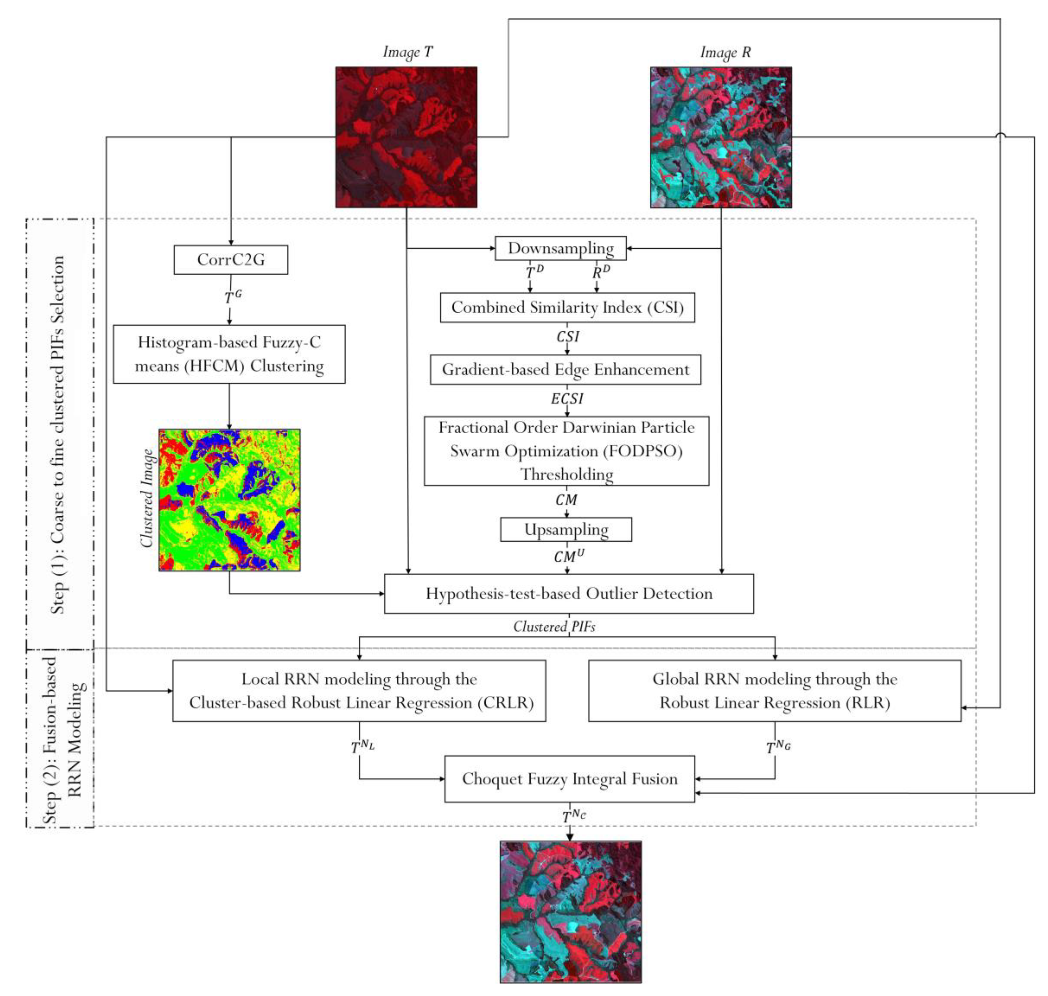
2.1. Proposed SRRN Method

Consider two co/geo-registered satellite images R (i.e., Equation (1)) and T (i.e., Equation (2)), respectively, as the reference and target images with the same size, acquired from the same scene at different times.

$$R=\left\{R\left(i,j,b\right)|1\le i\le H,1\le j\le W,1\le b\le N \right\}$$

(1)

$$T=\left\{T\left(i,j,b\right)|1\le i\le H,1\le j\le W,1\le b\le N \right\}$$

(2)

where H × W refers to height and width in pixels, and N is the number of spectral bands of the images R and T. The primary goal of this research was to generate a dependable normalized target image $T^{N_{\mathcal{C}}}$ (i.e., Equation (3)) computed using clustered PIFs extracted from input images R and T so that it is spectrally balanced with the reference image R.

$$T^{N_{\mathcal{C}}}=\left\{T^{N_{\mathcal{C}}}\left(i,j,b\right)|1\le i\le H,1\le j\le W,1\le b\le N \right\}$$

(3)

We designed a novel RRN framework composed of two main steps to reach this goal, as shown in Figure 1. First, the clustered PIFs were selected and optimized through a coarse-to-fine no-change selection strategy. The selected PIFs were then used in fusion-based RRN modeling to generate an optimal normalized target image. The steps included are detailed in the following sections.

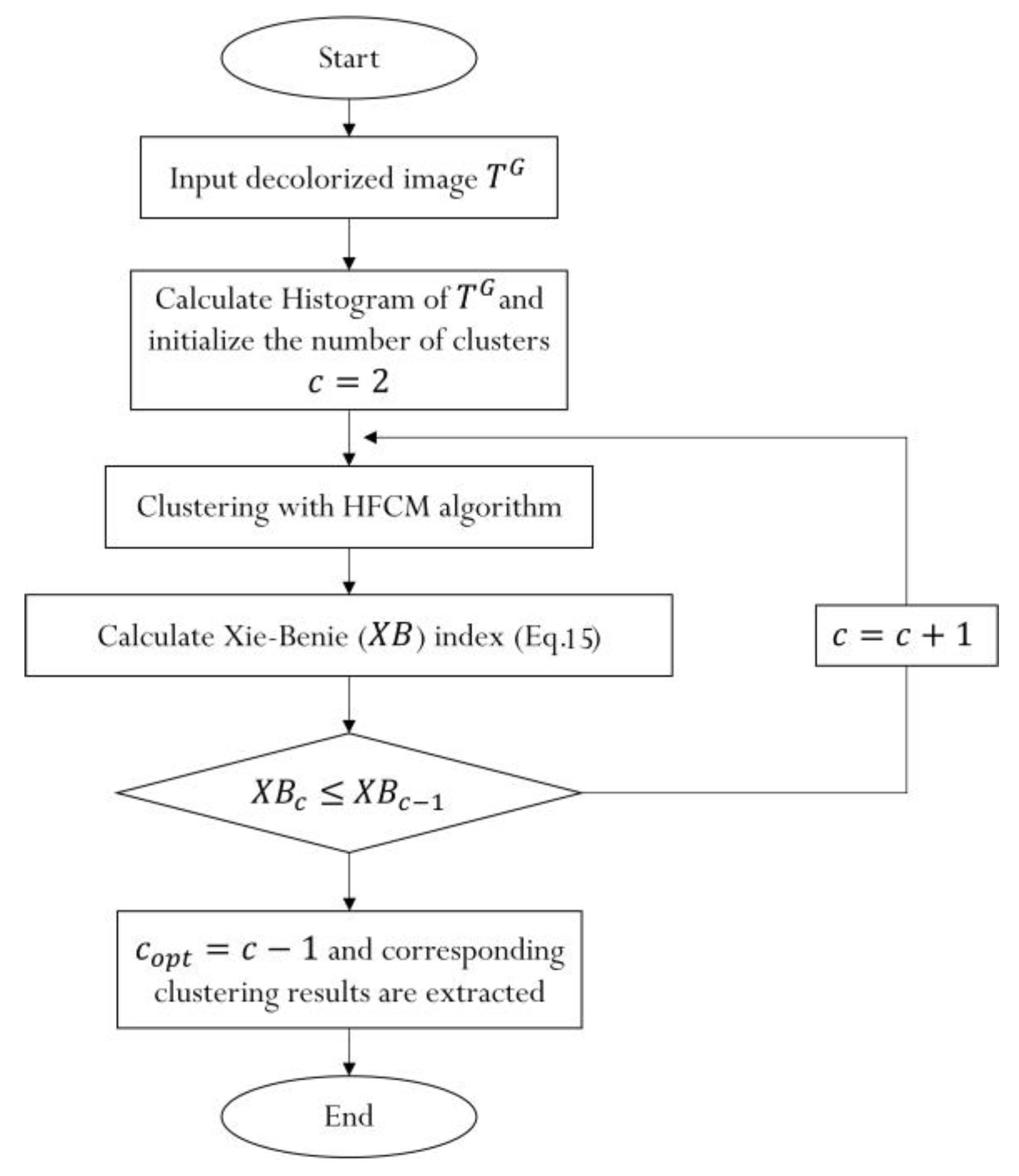
2.1.1. Step 1: Coarse-to-Fine Clustered PIFs Selection

As mentioned before, the first step of the proposed method was to generate reliable and well-spatially distributed PIFs from input images R and T over a coarse-to-fine no-change selection. To this end and for further faster processing, the grid size of input images was reduced to a coarser size P × Q, i.e.,

$$P=\lfloor sH\rfloor +1, Q=\lfloor sW\rfloor +1$$

(4)

where the operator $\lfloor .\rfloor$ rounds its argument toward the nearest integer, s is the scaling factor of down-sampling, computed by

$$s=min\left(\frac{\phi }{min\left(W,H\right)},\frac{min\left(W,H\right)}{max\left(W,H\right)}\right),$$

(5)

where φ is the user-defined positive integer (e.g., 128, 512, 720), min(.) and max(.) are respectively minimum and maximum operators. Accordingly, the input images R and T were down-sampled, respectively, to $R^D$ and $T^D$ which are defined as follows:

$$R^D=\left\{R^D\left(p,q,b\right)|1\le p\le P,1\le q\le Q,1\le b\le N\right\}$$

(6)

$$T^D=\left\{T^D\left(p,q,b\right)|1\le p\le P,1\le q\le Q,1\le b\le N \right\}$$

(7)

To generate a dependable input for the no-change selection process, down-sampled images $T^D$ and $R^D$ were then compared through a similarity index CSI which was combined from three metrics as follows:

$$CSI=\frac{\rho +\left(1-D^{Ch}\right)+\left(1-\theta \right)}{3}$$

(8)

where ρ, $D^{Ch}$, and θ respectively refer to Pearson correlation, Chebyshev distance, and SAM [35] metrics, which are given by:

$$D^{Ch}\left(p,q\right)=ma{x}_b\left|T_b^D\left(p,q\right)-R_b^D\left(p,q\right)\right|, b=1,2,\dots ,N$$

(9)

$$\rho \left(p,q\right)=\frac{{{\displaystyle \sum }}_{b=1}^N\left(T_b^D\left(p,q\right)-\overline{T_b^D}\right)\left(R_b^D\left(p,q\right)-\overline{R_b^D}\right)}{\sqrt{{{\displaystyle \sum }}_{b=1}^N{\left(T_b^D\left(p,q\right)-\overline{T_b^D}\right)}^2}\sqrt{{{\displaystyle \sum }}_{b=1}^N{\left(R_b^D\left(p,q\right)-\overline{R_b^D}\right)}^2}}, b=1,2,\dots ,N$$

(10)

$$\theta \left(p,q\right)=co{s}^{-1}\left(\frac{{{\displaystyle \sum }}_{b=1}^N{T}_b^D\left(m,n\right)R_b^D\left(m,n\right)}{\sqrt{{{\displaystyle \sum }}_{b=1}^N{T}_b^D{\left(p,q\right)}^2}\sqrt{{{\displaystyle \sum }}_{b=1}^N{R}_b^D{\left(p,q\right)}^2}}\right), b=1,2,\dots ,N$$

(11)

where $T_b^D\left(p,q\right)$ and $R_b^D\left(p,q\right)$ represent the gray-level pixel (p, q) in the spectral band bth of the down-sampled target and reference images, respectively. Such a combination can better reflect the characteristics of the changed and unchanged areas because it compares the reference and target images from different perspectives. It is worth noting that each metric was rescaled to [0, 1] by the Min-Max method before they were used in constructing $CSI$.

To reinforce the boundaries of the changed/unchanged regions in the index CSI, gradient magnitude of the index was first calculated as:

$$Gma{g}_{CSI}=\left|\nabla \left(G_{\sigma }*CSI\right)\right|$$

(12)

where $G_{\sigma }*CSI$ stands for the convolution of the CSI index with a Gaussian smoothing kernel $G_{\sigma }$, and ∇ denotes the gradient operator. The maximum operator was then used to supply complementary information from the index CSI and its gradient magnitude $Gma{g}_{CSI}$ into the enhanced index ECSI which is given by:

$$ECSI\left(p,q\right)=max \left(CSI\left(p,q\right),Gma{g}_{CSI}\left(p,q\right)\right),$$

(13)

The ECSI index makes a trade-off between geometrical detail preserving (edges and corners) and enhancing changed regions. It should be noted that $Gma{g}_{CSI}$ rescaled to [0, 1] before applying the max operator.

Generally, due to the coarse resolution of ECSI and the complexity of land surface features, a binary segmentation result often fails to reflect the real changed/unchanged regions. To address this issue, an automatic multilevel thresholding was applied to the index CSI to generate the change map $CM=\left\{\mathrm{cm}\left(p,q\right)\in \left\{0,1,2\right\}|1\le p\le P,1\le q\le Q \right\},$ in which $\mathrm{cm}\left(p,q\right)\in \left\{0,1,2\right\}$, (“0” and “1” indicate the pixel respectively belongs to the certain changed and unchanged classes, whereas “2” involves pixels belonging to the uncertain class. This process can be performed as follow:

$$CM\left(p,q\right)=\{\begin{array}{c}0, if CSI\left(p,q\right)<T{h}_1\\ 1, if CSI\left(p,q\right)>T{h}_2\\ 2, else \end{array}$$

(14)

where the low and high thresholds, $T{h}_1$ and $T{h}_2$ were determined by the fractional-order Darwinian particle swarm optimization (FODPSO) thresholding [36] due to its efficiency and fast process. The change map, CM, was further up-sampled to the original size of input images using the nearest-neighbor interpolation and indexed by $C{M}^U$.

In fine no-change selection, a local outlier detection was introduced, inspired by [37], to select reliable and well-spatially distributed PIFs from different LULCs by making decisions based on a hypothesis test. To this end, the target image T, was first converted to the grayscale target image$T^G,$ using CorrC2G [38], and it then partitioned into the $c$ cluster. Since satellite image typically includes multiple features with overlapped distributions, fuzzy clustering algorithms have been found to be very beneficial [39,40]. In this study, the HFCM clustering [32] was selected for this task because it operates on the histogram of an input image instead of the entire image, leading to a much faster process and reducing memory storage. The HFCM algorithm typically needs to know the number of clusters as an input which should be optimally determined. In this study, the optimum number of clusters $\left(c_{opt}\right)$ was self-adaptively selected during the analysis of the Xie-Beni (XB) index [41] (i.e., Equation (15)) as the workflow of Figure 2.

$$XB=\frac{{{\displaystyle \sum }}_{c=1}^{c_n}{{\displaystyle \sum }}_{l=1}^L{u}_{cl}^m h\left(l\right)d^2\left(l,{\upsilon }_c\right)}{L mi{n}_{c,z=1,2,\dots ,c_n c\ne z}{d}^2\left({\upsilon }_z,{\upsilon }_c\right)}$$

(15)

where

$$u_{cl}=\frac{1}{{{\displaystyle \sum }}_{z=1}^{c_n}{\left(\frac{d^2\left(l,{\upsilon }_c\right)}{d^2\left(l,{\upsilon }_z\right)}\right)}^{\frac{2}{m-1}}}$$

(16)

and

$${\upsilon }_c=\frac{{{\displaystyle \sum }}_{l=1}^L{u}_{cl}^m h\left(l\right)l}{{{\displaystyle \sum }}_{l=1}^L{u}_{cl}^m }$$

(17)

where $h\left(l\right)={\left\{h\left(l\right)\right\}}_{l=1,2,...,L}$ is the histogram of the image $T^G$ with L gray-levels, i.e., $L=max\left(T^G\right)$; $d\left(.,.\right)$ is the distance metric between two variables, $c_n$ is the cluster number, the membership function $u_{cl}$ (i.e., Equation (16)) and cluster center ${\upsilon }_c$ (i.e., Equation (17)) are obtained as a result of applying the HFCM algorithm to the image $T^G$. It is worth noting that each pixel value of the image $T^G$ was normalized according to Equation (18) to make sure that they are in the range of [0, 255], i.e., $T^G\left(i,j\right)\in \left[0,255\right]$:

$$T^G\left(i,j\right)=\lfloor \frac{T^G\left(i,j\right)-min\left(T^G\right)}{max\left(T^G\right)-min\left(T^G\right)}\times 255\rfloor$$

(18)

After partitioning the image $T^G$ into $c_{opt}$ clusters, the pixel pairs of input images belonging to the unchanged class were first picked up from each cluster and considered as the definite PIFs for that cluster. The hypothesis-test-based method was then proposed to eliminate the outliers from pixels of the uncertain class in each cluster using statistical parameters estimated based on the definite PIFs. As a result of this process, more reliable PIFs could be extracted in each cluster, resulting in accurate modeling between the reference and target images.

Let’s consider that in each cluster, $R_{u/c}$ and $T_{u/c}$ are a vector of pixels values that belong to the uncertain class in each spectral band of reference and target images, respectively. Moreover, suppose that they follow a BVN distribution, and their joint probability density function (PDF) can be formulated as follows:

$$f\left(Z_{u/c}\right)=\frac{1}{2\pi {\left|\mathsf{\Sigma }\right|}^{0.5}}{e}^{-0.5\left[{\left(Z_{u/c}-\mu \right)}^{\prime }{\mathsf{\Sigma }}^{-1}\left(Z_{u/c}-\mu \right)\right]},$$

(19)

where $Z_{u/c}{}^T=\left(R_{u/c},T_{u/c}\right)$ and $\mu$ and $\mathsf{\Sigma }$ are, respectively, the mean vector and covariance matrix generated from $R_{u/c}$ and $T_{u/c}$ in each cluster. Moreover, as is clear from Equation (19), ${\left(Z_{u/c}-\mu \right)}^{\prime }{\mathsf{\Sigma }}^{-1}\left(Z_{u/c}-\mu \right)$ represent the Mahalanobis distance of input samples, following a chi-square distribution with 2 degrees of freedom. Accordingly, the probability contour of the BVN distribution can be defined for each cluster as follows:

$${\left(Z_{u/c}-\mu \right)}^{\prime }{\mathsf{\Sigma }}^{-1}\left(Z_{u/c}-\mu \right)=\xi$$

(20)

where ξ is the scale of the probability contour and determined as $\xi ={\chi }_{1-\varrho ,2}^2$, in which $\varrho$ is a given level of significance (e.g., the 95% probability contour corresponds to $\varrho =0.05$ level of significance).

As can be seen from Equation (20), the performance of the probability contour is highly dependent on the estimation of its statistical parameters (i.e., $\mu$ and $\mathsf{\Sigma }$). The uncertain class may include many noises and anomalies in each cluster, leading to incorrect statistical parameters estimation and distortion of RRN results. To address this problem, we used unchanged samples (i.e., definite PIFs) to correctly estimate the statistical parameters of μ and Σ for each cluster. Therefore, the probability contour at the given significance level was updated with such parameters and then directly adopted to form the critical region for the hypothesis test in each cluster. For each cluster, the hypothesis had a null hypothesis ${\mathrm{H}}_0:{\left(Z_{u/c}-\mu \right)}^{\prime }{\mathsf{\Sigma }}^{-1}\left(Z_{u/c}-\mu \right)\le \xi ,$ i.e., all of the uncertain pixel values which fall inside the critical region added to the set of PIFs in the corresponding band. Since this process was implemented band-by-band, a majority voting rule over spectral bands produced the final decision for selecting PIFs from uncertain pixels in each cluster.

2.1.2. Step 2: Fusion-Based RRN Modeling

This step aimed to adjust the target image to the reference image through a novel fusion-based RRN modeling. To this end, two normalized images of $T^{N_G}$ and $T^{N_L}$ were first generated, respectively, through the global and local RRN modeling based on the clustered PIFs. In fact, the relation between the target and reference images was once modeled globally through a band-by-band RLR as follows:

$$T_b^{N_G}={\alpha }_b^G{T}_b+{\beta }_b^G$$

(21)

where ${\alpha }_b^G$ and ${\beta }_b^G$ are respectively the global slope and intercept for the $b$th spectral band, which were estimated using the iteratively reweighted least-squares (IRLS) method [42] based on the gray-levels of the clustered PIFs in images, T and R. The process of the IRLS method was started by considering the initial value for ${\alpha }_b$ and ${\beta }_b$. At each iteration τ, the non-negative weights ${\psi }_b^{\left(\tau -1\right)}$ of clustered PIFs were then estimated from the previous iteration based on the bisquare estimator [43]. In the next stage, the new coefficients were estimated as follows:

$${\alpha }_b^G{}^{\left(\tau \right)}=\frac{{{\displaystyle \sum }}_{y=1}^{N_{\mathrm{PIF}}}{\psi }_{b,y}^{\left(\tau -1\right)}\left(t_{b,y}-{\tilde{\mu }}_{t_b}{}^{\left(\tau -1\right)}\right)\left(r_{b,x}-{\tilde{\mu }}_{r_b}{}^{\left(\tau -1\right)}\right)}{{{\displaystyle \sum }}_{y=1}^{N_{\mathrm{PIF}}}{\psi }_{b,y}^{\left(\tau -1\right)}{\left(t_{b,y}-{\tilde{\mu }}_{t_b}{}^{\left(\tau -1\right)}\right)}^2}$$

(22)

$${\beta }_b^G{}^{\left(\tau \right)}={\tilde{\mu }}_{r_b}{}^{\left(\tau -1\right)}-{\alpha }_b^G{}^{\left(\tau \right)}{\tilde{\mu }}_{t_b}{}^{\left(\tau -1\right)}$$

(23)

where $N_{PIF}$ is the total number of clustered PIFs, $t_{b,y}$ and $r_{b,y}$ are respectively the gray-levels for the $y$th clustered PIF on the $b$th spectral band of images T and R; ${\tilde{\mu }}_{t_b}{}^{\left(\tau -1\right)}$ and ${\tilde{\mu }}_{r_b}{}^{\left(\tau -1\right)}$ are the weighted means of gray-levels of clustered PIFs in the bth spectral band of images T and R, respectively, which are calculated from the previous iteration as follows:

$${\tilde{\mu }}_{t_b}{}^{\left(\tau -1\right)}=\frac{{{\displaystyle \sum }}_{y=1}^{N_{\mathrm{PIF}}}{\psi }_{b,y}^{\left(\tau -1\right)}{t}_{b,y}}{{{\displaystyle \sum }}_{y=1}^{N_{\mathrm{PIF}}}{\psi }_{b,y}^{\left(\tau -1\right)}}$$

(24)

$${\tilde{\mu }}_{r_b}{}^{\left(\tau -1\right)}=\frac{{{\displaystyle \sum }}_{y=1}^{N_{\mathrm{PIF}}}{\psi }_{b,y}^{\left(\tau -1\right)}{r}_{b,y}}{{{\displaystyle \sum }}_{y=1}^{N_{\mathrm{PIF}}}{\psi }_{b,y}^{\left(\tau -1\right)}}$$

(25)

The two last stages were repeated until the estimated normalization coefficients converged to optimal values.

The RLR is much more robust to existing outliers than the other conventional linear regression models due to an efficient weighting function in its procedure [42]. The global RRN modeling generates a uniform normalized image where the discontinuity problem is not observed. However, applying such an approach may be insufficient to model the complex relationship between target and reference images, especially in dealing with datasets with different LULC types. Additionally, when the number of PIFs in one of the clusters is high, the global RRN modeling results may be biased to that cluster. To address these problems, the CRLR was introduced as a local RRN modeling to locally estimate the relation between image pairs in a band-by-band manner, which is defined as

$$T_b^{N_L}=\frac{{{\displaystyle \sum }}_{c=1}^{c_{opt}}{W}_{b,c}\left({\alpha }_{b,c}^L{T}_b+{\beta }_{b,c}^L\right)}{{{\displaystyle \sum }}_{c=1}^{c_{opt}}{W}_{b,c}}, c=1,2,..., c_{opt}$$

(26)

where ${\alpha }_{b,c}^L$ and ${\beta }_{b,c}^L$ are respectively the slope and intercept for $o$th cluster of the bth spectral band, which were calculated by the IRLS technique; $W_{b,o}$ refers to the weight matrix, which was separately computed for each cluster based on the inverse distance of pixel values of the target image from the corresponding cluster center as follows:

$$W_{b,c}\left(i,j\right)=\frac{1}{\parallel T_b\left(i,j\right)-{\upsilon }_c\parallel {}^2}, c=1,2,..., c_{opt}$$

(27)

Such an RRN model can generate a normalized image that is well adjusted to the reference image in different LULC. Furthermore, the weight matrix embedded in this model can help decrease the potential bias in the RRN results. However, the normalized image generated by the local model is not as uniform as that provided by the global model, where discontinuity along the LULC’s edge boundaries could be observed in the results of this model. Thus, the global and local RRN approaches include advantages and weaknesses in producing the normalized image. Accordingly, we looked for a strategy that decreases the discontinuity along the LULC’s edge boundaries and reduces the bias model problem. This could be resolved by fusing information from the normalized images $T^{N_G}$ and $T^{N_L}$. There are a variety of fusion approaches available in the literature for merging information from multiple sources. In this study, we used the Choquet integral operator [33] to construct the fused normalized image $T^{N_{\mathcal{C}}},$as it utilizes the fuzzy measures in its calculation, allowing it to consider all possible combinations of criteria in the decision-making process [44].

Suppose that we have $m$ normalized images, $T^N=\left\{T^{N_1},T^{N_2},...,T^{N_m}\right\},$ for fusion. Denote the gray-level of $k$th normalized image, $T_b^{N_k}$, on $n$th pixel in the $b$th spectral band, $x_{b,n}$, as $f\left(T_b^{N_k};x_{b,n}\right)$. The discrete Choquet integral on the instance, $x_{b,n},$ calculated by [45]:

$${\mathcal{C}}_g\left(x_{b,n}\right)={\displaystyle \sum }_{k=1}^m\left(f\left(T_b^{N_k};x_{b,n}\right)-f\left(T_b^{N_{k-1}};x_{b,n}\right)\right)g\left(A_k\right), 1<k<m$$

(28)

where ${\mathcal{C}}_g$ is rearranged so that $0\le f\left(T_b^{N_1};x_{b,n}\right)\le f\left(T_b^{N_2};x_{b,n}\right)\le ...\le f\left(T_b^{N_m};x_{b,n}\right), g\left(Ak\right)$ refer to the fuzzy measure element value corresponding to the subset $A_k$ =$\left\{T_b^{N_1},T_b^{N_2},...,T_b^{N_m}\right\}$, and $f\left(T_b^{N_1};x_{b,n}\right)=0$. Note that when $g$ is an $\lambda$-fuzzy measure, $g\left(Ak\right)$ values are determined by [34]:

$$g\left(Ak\right)=g\left(\left\{T_b^{N_k}\right\}\right)+g\left(\left\{T_b^{N_{k-1}}\right\}\right)+\lambda g\left(\left\{T_b^{N_k}\right\}\right)g\left(\left\{T_b^{N_{k-1}}\right\}\right), 1<k<m$$

(29)

where $g\left(\left\{T_b^{N_0}\right\}\right)=0$, the parameter $\lambda$ refers to the degree of interaction between two components which is obtained with the condition $g\left(T_b^{\mathrm{N}}\right)=1$ as the following equation [45]:

$$\lambda +1={\displaystyle \prod }_{k=1}^m\left(1+\lambda g\left(\left\{T_b^{N_k}\right\}\right)\right)$$

(30)

As for the fusion between two normalized images, $T^{N_G}$and $T^{N_L}$ the domain is defined as $T^N=\left\{T^{N_G},T^{N_L}\right\}$. In this domain and according to Equation (28), the pixel value for the fused image, $T^{N_{\mathcal{C}}},$ can be obtained as follows:

$$T_b^{N_{\mathcal{C}}}\left(x_{b,n}\right)=\{\begin{array}{c}f\left(T_b^{N_G};x_{b,n}\right)g\left(\left\{T_b^{N_G},T_b^{N_L}\right\}\right)+\left(f\left(T_b^{N_L};x_{b,n}\right)-f\left(T_b^{N_G}\right)\right)g\left(\left\{T_b^{N_L}\right\}\right), f\left(T_b^{N_G};x_{b,n}\right)\le f\left(T_b^{N_L};x_{b,n}\right)\\ f\left(T_b^{N_L};x_{b,n}\right)g\left(\left\{T_b^{N_L},T_b^{N_G}\right\}\right)+\left(f\left(T_b^{N_G};x_{b,n}\right)-f\left(T_b^{N_L}\right)\right)g\left(\left\{T_b^{N_G}\right\}\right), f\left(T_b^{N_G};x_{b,n}\right)>f\left(T_b^{N_L};x_{b,n}\right)\end{array}$$

(31)

where $g\left(\left\{T_b^{N_L}\right\}\right)$ and $g\left(\left\{T_b^{N_G}\right\}\right)$ are the fuzzy measures respectively for $f\left(T_b^{N_L};x_{\mathrm{b},n}\right)$ and $f\left(T_b^{N_G};x_{\mathrm{b},n}\right),$ which were determined based on the inverse of the absolute value of the gray-level difference between normalized and reference images on the $n$th pixel in the $b$th spectral band as follows:

$$g\left(\left\{T_b^{N_L}\right\}\right)=\frac{1}{\left|f\left(T_b^{N_L};x_{b,n}\right)-f\left(R_b;x_{b,n}\right)\right|}$$

(32)

$$g\left(\left\{T_b^{N_G}\right\}\right)=\frac{1}{\left|f\left(T_b^{N_G};x_{b,n}\right)-f\left(R_b;x_{b,n}\right)\right|}$$

(33)

By substituting $g\left(\left\{T_b^{N_L}\right\}\right)$ and $g\left(\left\{T_b^{N_G}\right\}\right)$into Equation (29), the joint fuzzy measure $g\left(\left\{T_b^{N_L},T_b^{N_G}\right\}\right)=g\left(\left\{T_b^{N_G},T_b^{N_L}\right\}\right)$ can be determined as follow:

$$g\left(\left\{T_b^{N_L},T_b^{N_G}\right\}\right)=g\left(\left\{T_b^{N_L}\right\}\right)+g\left(\left\{T_b^{N_G}\right\}\right)+\lambda g\left(\left\{T_b^{N_L}\right\}\right)g\left(\left\{T_b^{N_G}\right\}\right),$$

(34)

2.2. Datasets

As part of this study, a simulated dataset and four real bi-temporal optical images taken by Landsat-7, Terra, Sentinel-2, and IRS satellites were used to evaluate the proposed SRRN method (see Figure 3). The key reasons for choosing these datasets were their diversity in terms of satellite sensor, geographical coverage, and various atmospheric conditions. The main characteristics of real datasets are summarized in

Table 1. Characteristics of the datasets used in this study.

Dataset	Reference/Target	Satellite (Sensor)	Band Type	Resolution		Image Size (Pixels)	Date	Study Area
				Spatial (m)	Radiometric (Bits)
# 1	Reference	Landsat 7 (ETM+)	Blue, Green, Red, NIR *, SWIR * 1, SWIR 2	30	8	591 × 591	September 2002	Lago Mulargia lake, Cagliari, Italy
	Target						May 2003
# 2	Reference	Terra (ASTER)	Green/Yellow, Red, NIR SWIR 1, SWIR 2, SWIR 3, SWIR 4, SWIR 5, SWIR 6,	15/30	8	2000 × 2000	July 2002	Ahwaz, Khuzestan, Iran
	Target						July 2003
# 3	Reference	Sentinel 2 (MSI)	C/A *, Blue, Green, Red, VRE * 1, VRE 2, VRE 3, NIR, NIRn *, WV *, SWIR 1, SWIR 2	10/20/60	12	1500 × 1500	April 2016	Hamoon wetland, Iran-Afghanistan border
	Target						April 2018
# 4	Reference	IRS (LISSIII)	Green, Red, NIR	23.5	8	900 × 900	July 1998	Varzaqan, East Azerbaijan Province, Iran
	Target						May 2007

* C/A: coastal aerosol, VRE: vegetation red edge, NIR: near-infrared, NIRn: narrow NIR, SWIR: short wave infrared, WV: water-vapor.

.

The simulated dataset was made up of a portion of 1200 × 1200 pixels of an uncalibrated image acquired by the SPOT 7 satellite over the three channels (green, red, NIR) in November 2014 from Curitiba, Brazil, i.e., geographically limited between [24°34′18″ S, 49°43′44″ W] and [24°38′8″ S, 49°39′28″ W]. In this dataset, the uncalibrated image was considered as the target image, whereas its adjusted image (in terms of contrast and brightness) with some simulated changed areas was selected as the reference image (see Figure 3a,c first row). The target image includes the different cropland types with low contrast and brightness. Following RRN, the contrast and illumination of target images must be similar to those of the reference image, and croplands will be discernible similarly to those shown in simulated reference images.

Dataset 1 is composed of the bi-temporal Landsat 7 images over Lago Mulargia Lake in Italy (i.e., geographically limited between [39°45′01″ N, 9°9′30″ E] and [39°35′02″ N, 9°22′30″ E]) spanning a period of about one year (see Figure 3a,c second row). There are many differences among bitemporal data, including seasonal changes in different LULC, especially in vegetation, and varying illumination that could result in false changes in the final results of RS applications such as change detection and time series analysis. The Landsat 7 image acquired in September 2002 was considered the reference image because of its reasonable contrast and illumination. The one acquired in May 2003 was used as the target image due to its non-ideal spectral properties. As a result of RRN, the spectral response of various LULCs in the target image is expected to be similar to their response in the reference image.

Dataset 2 consists of the bi-temporal images acquired by the ASTER sensor over the south of Ahwaz, Iran (i.e., geographically limited between [31°20′04″ N, 48°10′02″ E] and [31°01′01″ N, 48°41′03″ E]) across a period of about two years (see Figure 3a,c third row). There are many croplands, vegetation, soil changes, and illumination differences among this bitemporal data. The ASTER image taken in July 2002 was used as the reference image because of its realistic illumination and spectral contents. The one acquired in July 2003 was considered the target image. After applying RRN, the target image is expected to be harmonized with the reference image in terms of contrast, brightness, and spectral content. It is worth noting that the spatial resolution of 30 m/pixel bands of the ASTER images was also sharpened to 15 m/pixel by the PCA-based PAN-sharpening algorithm [46].

Dataset 3 contains the bitemporal Sentinel 2 images over the Hamoon wetland, Iran-Afghanistan border (i.e., geographically limited between [31°35′38″ N, 60°57′42″ E] and [31°22′38″ N, 61°15′36″ E]) across a period of about two years (see Figure 3a,c forth row). These images were acquired in the same month but under different atmospheric conditions. There are significant water body changes as well as illumination variations caused by slightly different viewing angles among the bitemporal data. The Sentinel 2 image taken in April 2016 was employed as the reference image, and atmosphere, terrain, and cirrus corrections were performed on this image by the Sen2Cor model, which is available in SNAP software. The uncalibrated Sentinel 2 image (at processing Level-1C) acquired in April 2016 was also used as a target image. After applying RRN, the spectral content of the target image is intended to be rectified based on that of the reference image. Moreover, the spatial resolutions of 20 m/pixel and 60 m/pixel bands of the Sentinel 2 dataset were also enhanced to 10 m/pixel by the Sen2Res model [47], which is available in the Sentinel Application Platform (SNAP) open-source software.

Dataset 4 includes the bitemporal IRS images over Varzaqan, Iran (i.e., geographically limited between [38°40′24″ N, 46°29′25″ E] and [38°25′12″ N, 46°47′56″ E]) spanning a period of about ten years (see Figure 3a,c last row). There are many LULC changes as well as mountain offsets caused by different viewing angles among this bitemporal data. The IRS image taken in July 1998 was employed as the reference image due to its better brightness and contrast than the one acquired in May 2007. After applying RRN, the target image was expected to be well-adjusted with the reference image in terms of spectral content and visual point of view.

All spectral bands of image pairs, except the thermal, cirrus, and panchromatic bands, were used in the RRN process. The ground truth of the change maps, which is shown in Figure 3d, was generated by the post-classification comparison and manual analysis of the image pairs. It is worth noting that the unchanged pixels in these maps were considered for RRN validation (experiments of Section 3.1, Section 3.3, and Section 3.4) to have fair results.

2.3. Evaluation Metrics

To quantify the global performance of the proposed SRRN method and generate comparative experiments, the root mean square error (RMSE) was used in this study (Equation (35)).

$$\mathrm{RMSE}=\sqrt{\frac{1}{N_c}{\displaystyle \sum }_{\iota =1}^{N_c}{\left(R_{\iota }-T_{\iota }^N\right)}^2}$$

(35)

where $N_c$ is the total number of unchanged pixels in the binary change map. A low RMSE describes the acceptable RRN results.

To locally validate the performance of the proposed SRRN method, the cross-correlation (CC) to average mean absolute percentage error (AMAPE) ratio index (CAMRI) is suggested, which is calculated for each exciting LULC as follows:

$$\mathrm{CAMRI}=\frac{\mathrm{CC}}{\mathrm{AMAPE}}=\frac{\frac{{{\displaystyle \sum }}_{n_l=1}^{N_{c_l}}{{\displaystyle \sum }}_{b=1}^N\left(T_{n_l,b}^N-\overline{T_b^N}\right)\left(R_{n_l,b}-\overline{R_b}\right)}{\sqrt{{{\displaystyle \sum }}_{n_l=1}^{N_{c_l}}{{\displaystyle \sum }}_{b=1}^N{\left(T_{n_l,b}^N-\overline{T_b^N}\right)}^2}\sqrt{{{\displaystyle \sum }}_{n_l=1}^{N_{c_l}}{{\displaystyle \sum }}_{b=1}^N{\left(R_{n_l,b}-\overline{R_b}\right)}^2}}}{\frac{1}{N*N_{c_l}}{\displaystyle \sum }_{b=1}^N{\displaystyle \sum }_{n_l=1}^{N_{c_l}}\frac{\left|R_{b,n_l}-T_{b,n_l}^N\right|}{R_{b,n_l}}\times 100}$$

(36)

where $N_{c_l}$ denotes the number of test samples in a specific LULC, $\overline{R_b}$ and $\overline{T_b^N}$ are respectively the average values of these samples in the bth spectral band of the reference and normalized target images. The higher value of the CAMRI results in a better RRN.

3. Experimental Results

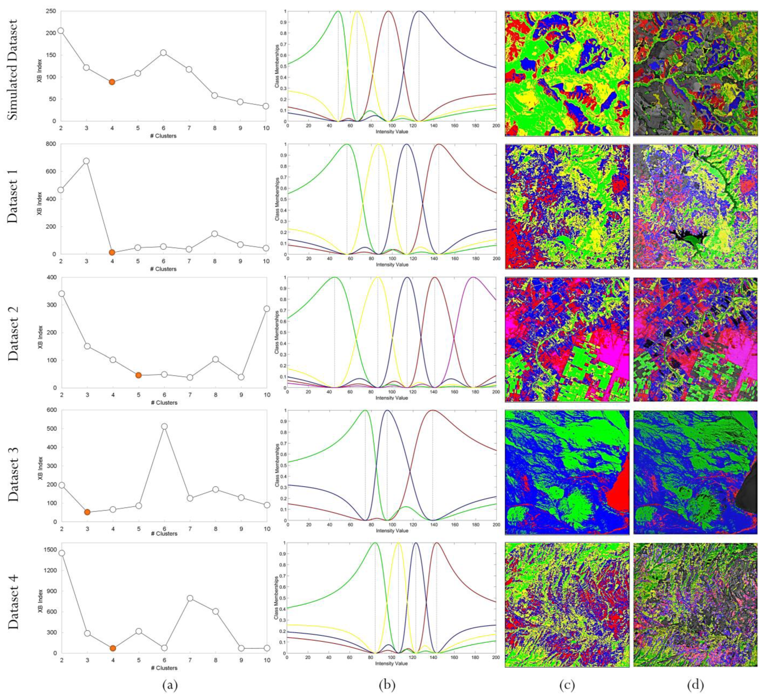
3.1. Analysis of the Coarse-to-Fine PIFs Selection

As clustering is an essential component in the proposed coarse-to-fine PIFs selection, we present the results of the HFCM algorithm for all datasets used in Figure 4a–c. In this way, the XB values for the number of clusters from 2 to 10 are shown in Figure 4a during the clustering process for each dataset. For the best cluster number in each dataset, the clustering results and membership maps are also shown in Figure 4b,c, whereas the selected PIFs in each cluster are illustrated in Figure 4d for all datasets.

As can be seen from the subplots in Figure 4a and according to the flowchart presented in Figure 2, the optimal cluster numbers were self-adaptively selected as 4, 4, 5, 3, and 4, respectively, for the simulated dataset and datasets 1–4. The achieved optimal cluster number for each dataset corresponds to the first minimum value of the XB index, which seemed to be consistent with the real number of clusters in the target image (see Figure 4b,c). As is evident from the clustering results and their membership maps, the decolorized target images were well categorized from dark to bright clusters. As a result, the robust and well-spatially distributed PIFs were collected from these clusters through the proposed hypothesis-test-based method, which was well fitted with the physical properties of ground surface types. For example, the clustered PIFs were extracted from dark and bright croplands of the simulated dataset using the proposed coarse-to-fine strategy (see Figure 4d first row). The PIFs were also collected from different LULC types of dataset 1, such as water bodies and wetlands (dark regions), dense vegetation (gray regions), sparse vegetation (light gray regions), and mountainous, as well as bare soil land cover (bright regions) (see Figure 4d second row). For dataset 2, the clustered PIFs mainly were selected from the river and dark-green farmlands (dark regions), wetlands (dark-gray regions), irrigated croplands (gray regions), harvested cropland areas (light-gray regions), and bare soil land covers (bright regions) (see Figure 4d third row). The clustered PIFs of dataset 3 were composed of the water bodies, sandy and rocky areas, and the dark, gray, and bright ground surfaces, respectively (see Figure 4d fourth row). They were also composed of dark to bright samples collected from the valleys, dense and sparse vegetation, and rocky areas included in dataset 4 (see Figure 4d last row).

To analyze the efficiency of the proposed coarse-to-fine strategy, its RRN results were compared to those obtained using the same approach without the downscaling process, without the hypothesis-test-based method, and when using CVA instead of CSI in terms of RMSE and computing time (Figure 5). The linear RLR was selected as the core of RRN modeling in this experiment to provide a fair comparison and investigate the quality of clustered PIFs generated by the coarse-to-fine approach under the mentioned conditions. The experiments and the computation time analysis were conducted on all considered datasets by MATLAB (version 2020a) on an Intel CPU Core (TM) i7-3770 GHz with 16 GB of RAM.

It is evident from bar charts Figure 5a–e that using CVA instead of CIS index in the proposed coarse-to-fine PIFs selection resulted in a significant reduction in RRN performance for most analyzed datasets. For example, the average RMSE was reduced by 7.37 and 0.05 in the best (simulated dataset) and worst (dataset 2) cases after using CVA instead of the CIS index, whereas it led to an increase in average RMSE by 0.42 only for dataset 3. These results could be due to the high sensitivity of CVA to radiometric differences between image pairs because it directly employs only information of spectral bands to generate a difference/change index. In contrast, the CSI index uses the integration of information obtained from distance, angle, and correlation between spectral bands of image pairs in the comparison process, which was less affected by radiometric distortions. However, the running time was reduced by almost 21% when using CVA in the PIF selection process, which could be due to the simplicity of CVA calculations (see Figure 5f).

After using the hypothesis-based test in the process of PIF selection, the average RMSEs were improved by 4.22% for the simulated dataset and 3.83%, 1.68%, 7.34%, and 1.05%, respectively, for datasets 1–4, indicating its efficacy in the PIF refinement (see Figure 5a–e). As expected, using a refinement algorithm raised the computational cost of the process. Knowing this, using a hypothesis-based-test algorithm increased the execution time of the proposed PIFs selection by almost 40% over most cases, which is worth considering for better results.

The PIFs selection without down-sampling yielded the best performance over most of the datasets, but there was no significant difference in its RRN accuracy and that of the proposed method. For example, when the down-sampling process was discarded from the proposed method, the average RMSE was reduced by only 0.11%. Furthermore, as compared to other approaches, the proposed PIF selection without down-sampling required the greatest processing time in all cases (see Figure 5f). These findings revealed that adopting down-sampling in the PIF selection process not only reduced execution time but also provided satisfactory RRN accuracy for most datasets.

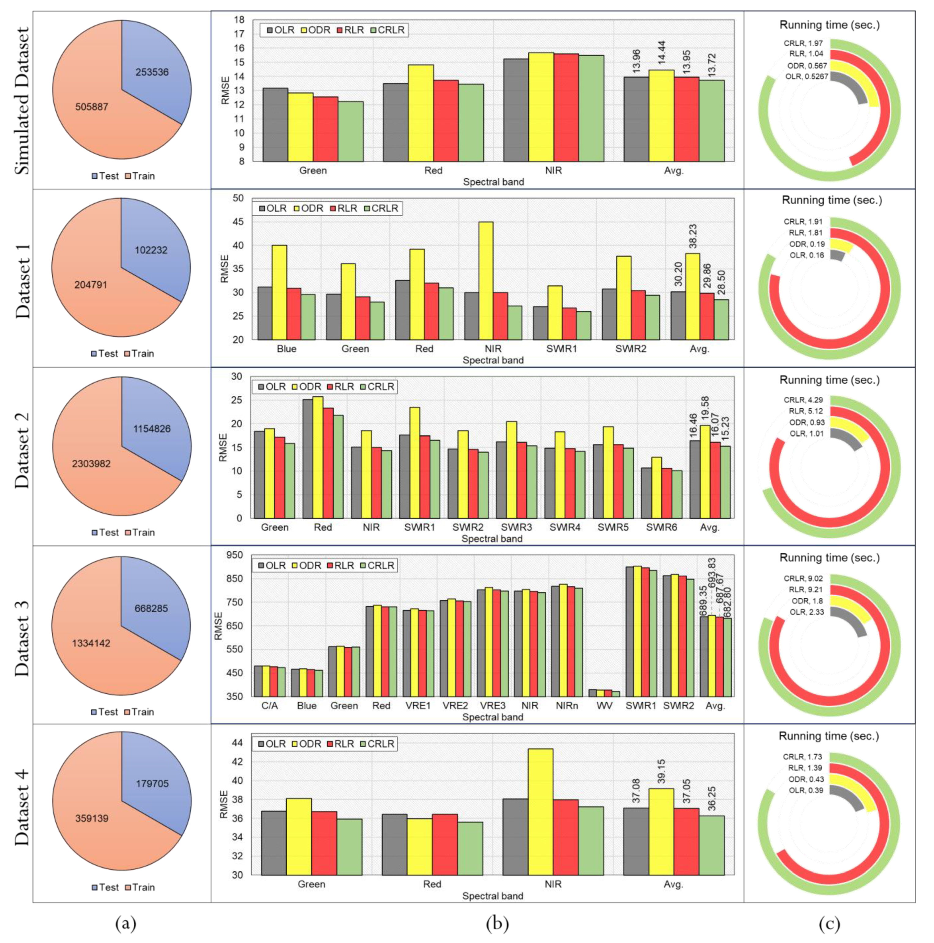
3.2. Comparative Results of the RRN Modelling

To evaluate the competence of the RLR and CRLR models, they were compared with the two most widely used models in the RRN process, including ordinary least squares (OLS) [48] and orthogonal distance regression (ODR) [49], in terms of RMSE and processing time (see Figure 6). For this experiment, 67% of the PIFs from each cluster were randomly selected for training, and the rest was used to test the models (see Figure 6a). In addition, we calculated the running time only for the modeling step (see Figure 6c).

As depicted in Figure 6b, the proposed CRLR model obtained the best performance in RRN modeling of all datasets among all considered models, which indicates its robustness and effectiveness in model fitting. For example, the CRLR outperformed the RLR, ORD, and OLR, respectively, by 5.20%, 22.19%, and 7.48% in the best case (dataset 2) and by ~1.5% in the worst cases (dataset 3) in terms of average RMSE. Moreover, RLR had a somewhat better performance than the OLR in that it slightly improved the average RMSE of the OLR by ~1% for all datasets. This can be mainly because RLR, like CRLR, benefits from the bisquare weighting function, resulting in more robust results. Among all considered models, the ORD had poor RRN results for considered datasets where it conducted somewhat large RMSE compared with other models. The main reason may be related to a large number of training samples and their variety of errors, leading to errors in fitting and estimating coefficients. Although the CRLR and RLR had better quantitative results than ORD and OLR, both of them were computationally intensive. This was more obvious for datasets 2 and 3, which have more spectral bands than other datasets (see Figure 6c). In summary, The CRLR and RLR typically require a much larger computational volume than conventional models used in the RRN modeling phase, which can be seen as a weakness of these models.

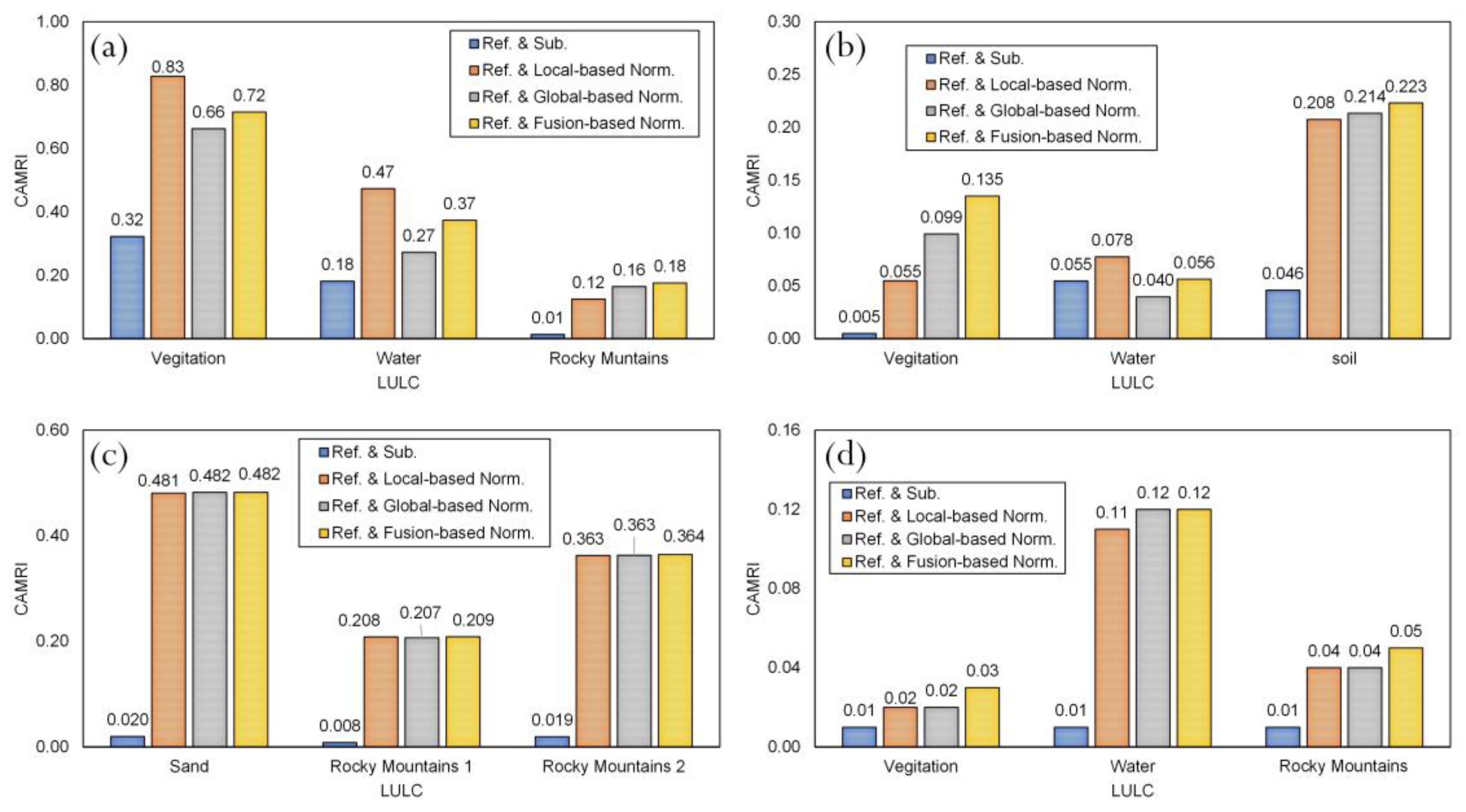
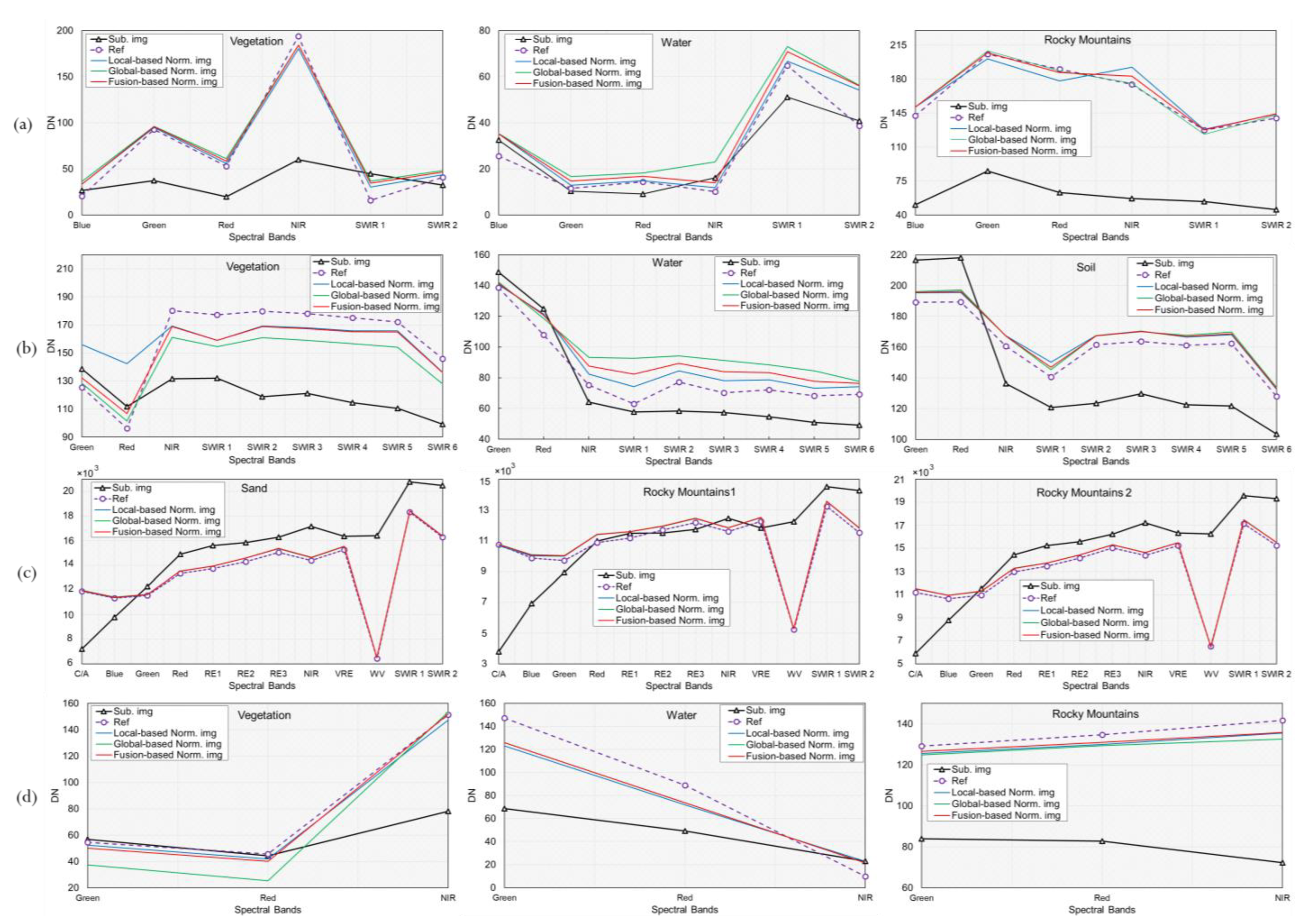
3.3. Effects of the Fusion-Based RRN Modelling

In this section, we evaluated the performance of the proposed fusion-based RRN model at the local and global levels over the analyzed datasets. The experiments were performed with the clustered PIFs selected by the proposed coarse-to-fine process. Figure 7 shows comparative results between the proposed fusion-based RRN model and local and RRN modeling in terms of accuracy and visual depth.

As demonstrated in Figure 7a–e, the normalized images produced by the proposed fusion strategy were more visually similar to the corresponding reference image than those generated by local and global models, indicating its effectiveness in the RRN process. Moreover, the proposed fusion-based strategy significantly reduced the amount of bias and discontinuities present in the normalized images of datasets 3 and 4, produced from local and global RRN models. For example, the local RRN modeling generated undesirable normalized images that were not well harmonized with the reference images in datasets 3 and 4, whereas global RRN modeling produced blurred normalized images. Notably, the fused normalized images in these two datasets were in good agreement with the relevant reference images (See Figure 7a–e second and third rows). On other datasets, there were not many visual differences between the normalized images generated by methods compared, where they all visually matched their reference images.

Based on the results illustrated in Figure 7e, the RMSEs were reduced over most of the spectral bands of the datasets after fusing the normalized images generated by the local and global models by the fuzzy Choquet integral. For example, when using the proposed fusion technique in RRN modeling instead of a single local model, like the cluster-wise RLR, the average RMSEs were reduced by 8.63% for the simulated dataset and 2.83%, 6.40%, 0.62%, and 1.69% for datasets 1–4, respectively. Moreover, the average RMSEs were improved by 1.90% for the simulated dataset and 8.84%, 3.57%, 1.06%, and 4.02%, respectively, for datasets 1–4 when the proposed fusion strategy in RRN modeling was used instead of the single global model like the RLR. This could mainly be due to the difference between the reference and normalized target images as the fuzzy Choquet integral memberships during the fusion process. In addition, local RRN modeling provided better results for datasets 1, 3, and 4, while global RRN modeling delivered better results for the simulated dataset and dataset 2. Based on our results, a single RRN model was not sufficient to achieve better qualitative and quantitative results, and a fused approach, such as the one proposed in this study, could lead to better results by optimally combining various normalized images.

The spectral characteristics of different LULC types in multi-temporal images may be unexpectedly affected due to radiometric distortions. Thus, a local assessment can be a practical approach to assessing the effectiveness of the proposed RRN methods in preserving spectral characteristics of LULC types on images pairs. In this way, the spectral signatures of several LULC types (e.g., vegetation, water, rock mountains) were compared before and after normalization using the proposed SRRN method under the local, global, and fused-based RRN modeling (see Figure 8). The CAMRI values before and after normalization were also compared over the LULC classes (see Figure 9). Multiple polygons from the LULC classes were manually selected for these experiments on the unchanged areas of reference, target, and normalized images.

As shown in Figure 8a–d, the spectral signatures of LULC types in the target images were well adjusted after normalization with the proposed SRRN method under different modeling. Moreover, these results were in good agreement with CAMRI values reported for datasets before and after RRN (see Figure 9a–d). In more detail, the spectral signatures of vegetation and water bodies in the normalized image generated by the local approach were slightly similar to those obtained in the reference image for dataset 1. The fusion-based method also had the best performance with a CMRI value of ~0.18 in rocky mountains areas of dataset 1. Similarly, the proposed fused approach provided spectrally better RRN results in the vegetation and soil LULC types, with the highest CMRI values. Nevertheless, the local model yielded better results for water bodies in dataset 2. The local, global, and fusion-based RRN modeling had the same performance for different LULCs included in dataset 3, as shown in Figure 8c and Figure 9c. Moreover, the local and global models also had nearly the same RRN performance for LULCs of dataset 4. In contrast, the proposed fusion-based model produced better results in spectral similarity and CAMRI values (see Figure 8d and Figure 9d).

Although the SRRN method under the mentioned models had locally acceptable results, small shifts were observed between the spectral signatures of some of the LULCs in the reference and normalized images. For example, such shifts were mainly observed in water bodies due to existing particles floating in these areas, such as phytoplankton, pollution, and sediments which affect the apparent color of the water between acquisition times of the reference-target image pair. Moreover, the differences between the spectral signatures of vegetation in the reference and normalized images were mostly observed for bi-temporal images acquired in different seasons (e.g., datasets 1, 2, and 4). This could be mainly due to differences in vegetation phenological properties.

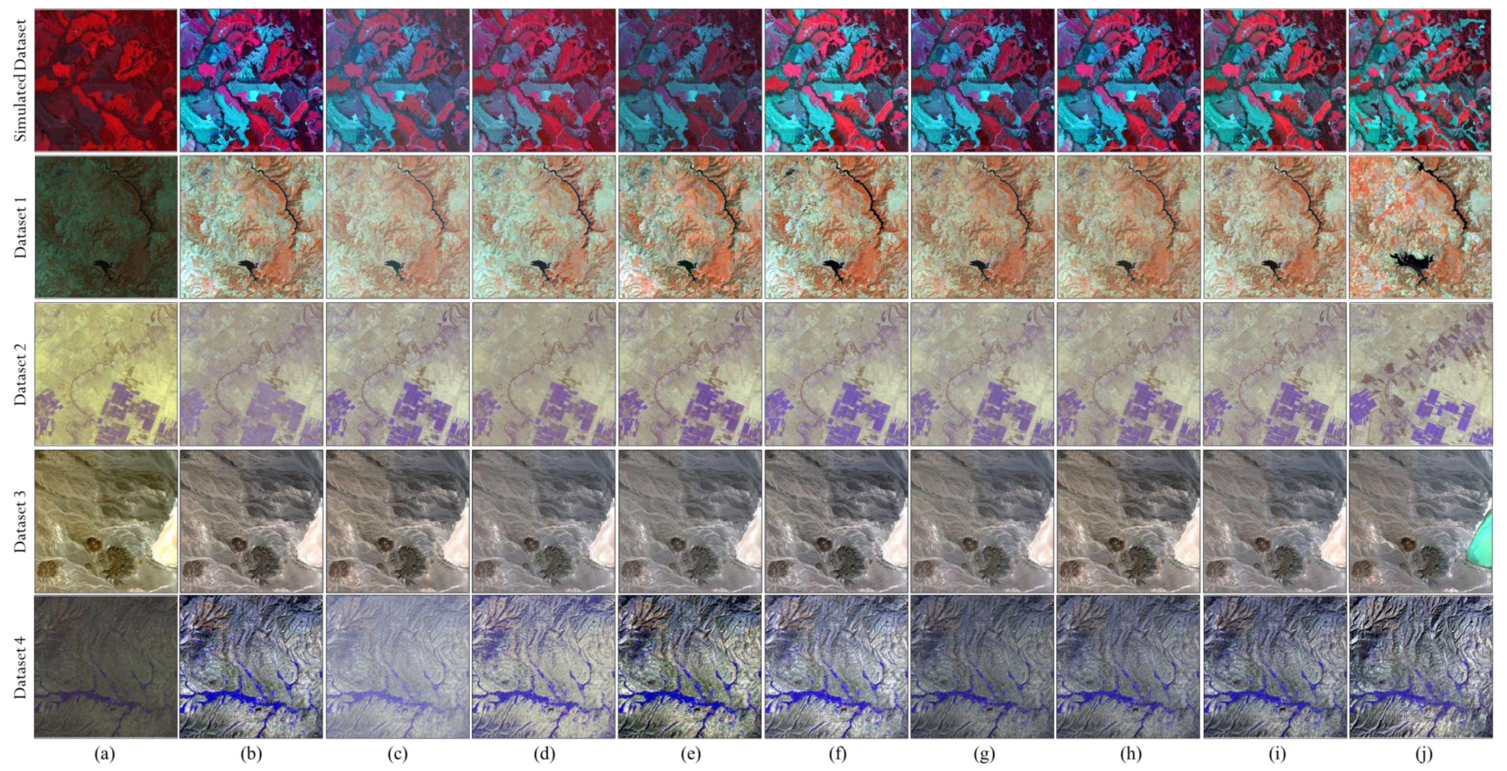
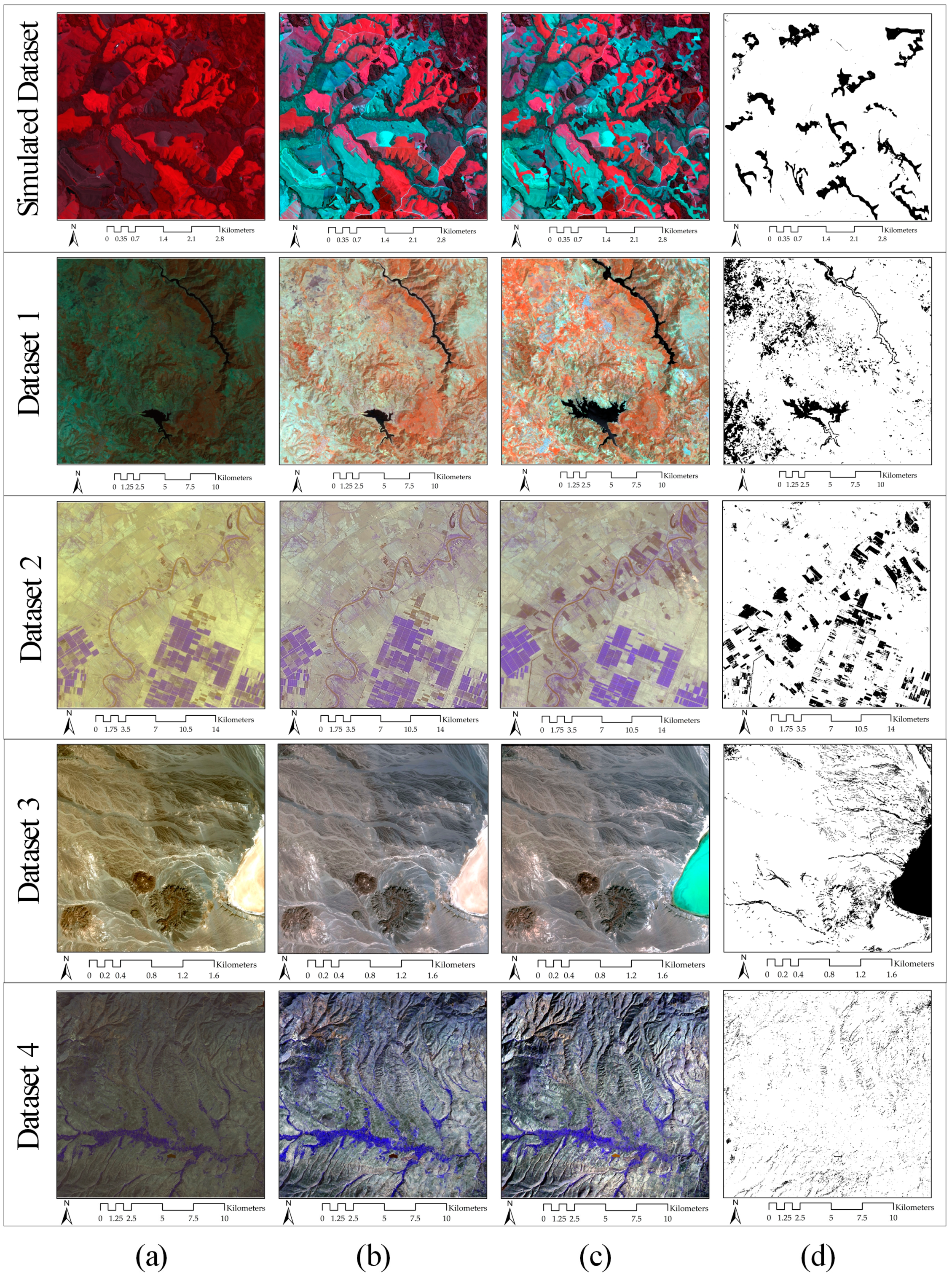
3.4. Comparative Results of the SRRN Methods

To evaluate the efficiency of the proposed method, it was compared with our implementations of IRMAD [15], multi-Otsu-based [29], MPIF [22], ASCRRF-based [27], GMM-EE [24], HOG-based [31], and FLSM-based [3] in terms of quantitative and qualitative results, as well as operation time (see

Table 2. Comparison between the accuracy and componential time of different SRRN methods and the proposed method for the simulated dataset.

Method	RMSE				Comp. Time (s)
	Green	Red	NIR	Avg.
Raw 1	87.50	65.49	54.41	69.13	----
IRMAD [15]	22.07	28.84	21.01	23.97	8.16
Multi-Otsu-based [29]	34.97	46.85	41.33	41.05	7.83
MPIF [22]	18.09	29.80	28.80	25.56	8.77
ASCR-RF-based [27]	13.28	13.81	19.32	15.47	15.96
GMM-EE [24]	14.28	16.71	19.44	16.81	11.03
HOG-based [31]	12.59	16.51	9.36	12.82	----
FLSM-based [3]	16.19	16.92	12.31	15.14	14.44
Proposed Method	8.69	10.52	8.71	9.31	7.54

¹ The results without applying any SRRN method.

,

Table 3. Comparison between the accuracy and componential time of different SRRN methods and the proposed method for dataset 1.

Method	RMSE							Comp. Time (s)
	Blue	Green	Red	NIR	SWIR1	SWIR2	Avg.
Raw 1	63.84	80.96	79.80	121.17	95.41	91.72	88.82	----
IRMAD [15]	29.69	26.30	29.00	29.00	20.14	25.78	26.65	10.44
Multi-Otsu-based [29]	36.21	33.95	41.73	24.19	24.71	32.44	32.20	09.61
MPIF [22]	32.50	27.56	30.28	35.25	21.34	26.90	28.97	17.21
ASCR-RF-based [27]	58.39	40.29	37.91	25.58	23.93	29.00	35.85	21.02
GMM-EE [24]	30.81	28.57	31.50	23.44	22.61	28.52	27.57	14.94
HOG-based [31]	36.84	30.51	32.95	27.97	22.70	28.93	29.98	----
FLSM-based [3]	30.83	27.18	29.83	23.82	21.02	27.06	26.62	26.19
Proposed Method	26.60	23.53	25.76	21.59	18.78	23.68	23.32	10.04

¹ The results without applying any SRRN method.

,

Table 4. Comparison between the accuracy and componential time of different SRRN methods and the proposed method for dataset 2.

Method	RMSE										Comp. Time (s)
	Green	Red	NIR	SWIR1	SWIR2	SWIR3	SWIR4	SWIR5	SWIR6	Avg.
Raw 1	21.02	25.33	34.17	31.23	45.37	42.22	45.73	47.65	32.38	36.12	----
IRMAD [15]	14.54	19.99	15.84	19.53	15.74	16.44	15.20	15.34	12.44	16.12	30.12
Multi-Otsu-based [29]	19.06	26.21	20.47	22.84	20.14	21.36	19.88	20.20	15.38	20.62	29.11
MPIF [22]	14.92	21.39	18.45	22.37	18.08	19.05	17.59	17.80	14.05	18.19	40.01
ASCR-RF-based [27]	14.41	19.73	18.94	21.81	18.72	19.48	18.17	18.32	14.85	18.27	79.23
GMM-EE [24]	14.08	19.18	15.06	17.69	14.99	15.65	14.65	14.86	12.03	15.36	58.24
HOG-based [31]	14.49	18.83	13.44	16.24	13.25	14.20	13.13	13.58	10.26	14.16	----
FLSM-based [3]	14.35	19.48	16.30	18.72	16.19	16.98	15.85	16.17	12.90	16.33	95.26
Proposed Method	11.44	15.46	13.98	16.63	13.89	14.43	13.49	13.47	10.86	13.74	33.26

¹ The results without applying any SRRN method.

,

Table 5. Comparison between the accuracy and componential time of different SRRN methods and the proposed method for dataset 3.

Method	RMSE													Comp. Time (s)
	C/A	Blue	Green	Red	VRE1	VRE2	VRE3	NIR	NIRn	WV	SWIR1	SWIR2	Avg.
Raw 1	5500.07	2252.14	1067.89	1462.33	1633.91	1370.60	1229.10	2394.21	1141.94	9264.19	2160.05	3676.26	2762.72	-----
IRMAD [15]	452.08	416.01	496.92	630.05	603.69	638.38	678.13	670.13	675.69	320.18	699.54	675.56	579.70	49.13
Multi-Otsu-based [29]	425.76	395.79	483.96	624.07	600.28	637.34	676.82	668.39	673.77	316.34	698.23	674.20	572.91	38.52
MPIF [22]	571.85	431.84	526.36	688.72	660.53	679.83	734.87	727.90	733.21	550.00	1132.36	784.99	685.21	42.94
ASCR-RF-based [27]	466.67	433.55	538.84	703.77	686.28	734.56	783.50	763.71	789.24	364.08	845.11	814.73	660.34	91.64
GMM-EE [24]	476.98	452.91	526.46	653.95	631.63	668.90	706.77	699.98	703.79	381.20	730.77	707.50	611.74	62.01
HOG-based [31]	1321.10	706.17	635.19	745.97	707.52	772.86	809.06	806.86	832.37	393.73	810.76	724.95	772.21	----
FLSM-based [3]	432.02	402.04	485.44	628.45	606.96	647.15	686.70	678.78	685.01	328.16	711.78	686.10	581.55	114.23
Proposed Method	421.15	389.92	482.63	621.99	598.18	634.77	673.96	664.97	669.78	312.80	693.43	668.66	569.35	45.88

¹ The results without applying any SRRN method.

and

Table 6. Comparison between the accuracy and componential time of different SRRN methods and the proposed methods for simulated dataset 4.

Method	RMSE				Comp. Time (s)
	Green	Red	NIR	Avg.
Raw 1	55.60	58.83	76.86	63.77	----
IRMAD [15]	40.08	40.20	42.14	40.81	6.15
Multi-Otsu-based [29]	46.18	45.91	48.39	46.82	6.08
MPIF [22]	44.36	43.73	42.93	43.67	6.19
ASCR-RF-based [27]	41.14	47.32	49.62	46.02	8.96
GMM-EE [24]	37.54	37.42	39.07	38.01	8.29
HOG-based [31]	38.20	38.56	42.31	39.69	---
FLSM-based [3]	40.61	39.13	41.78	40.51	13.65
Proposed Method	34.22	34.18	36.26	34.88	5.93

¹ The results without applying any SRRN method.

and Figure 10). These SRRN algorithms were set up as described in their respective works of literature. This study did not report the componential time of the HOG-based [31] SRRN technique since it is a semi-supervised SRRN approach that requires training data for its classification process.

As can be seen from Table 2, Table 3, Table 4, Table 5 and Table 6, RMSE values were significantly reduced after applying all considered SRRN methods over all datasets. Among these models, the proposed method obtained the highest accuracy in minimizing radiometric errors from the target images of the analyzed datasets. Specifically, the average raw RMSEs decreased significantly from 69.13 to 9.31 (~87%), from 88.82 to 23.32 (~74%), from 36.12 to 13.74 (~62%), from 2762.72 to 569.35 (~79%), and from 63.77 to 34.88 (~45%), respectively for the simulated dataset, and datasets 1–4. Compared with the implemented methods, the proposed methods also improved the average RMSEs by ~27% and ~1% in best and worst cases, i.e., the simulated dataset and dataset 3, respectively. This was mainly because the proposed method took advantage of the efficient coarse-to-fine PIFs selection and fusion-based RRN modeling in its process.

The multi-Otsu-based [29] had the worst RRN performance in most cases, except for dataset 3, in which the HOG-based [31] achieved a lower average RMSE compared with other well-known methods. This could be mainly because this method uses the Otsu thresholding as segmentation in its process, which is highly sensitive to the non-uniform illumination and imperfectly segment images with such distortions. The ASCRRF-based [27] also had an almost poor RRN performance in most cases because it uses the RF regression in RRN modeling, which is highly prone to overfitting and needs parameter tuning for each dataset. Although the MPIF [22] had a moderate RRN performance, it could not perfectly handle radiometric falsifications between image pairs in most cases, as shown in Table 2, Table 3, Table 4 and Table 5. This may be related to using several threshold-based sampling rules in PIFs selection that do not take LULC types into account, resulting in insufficient PIFs with an unsuitable spatial distribution.

The IRMAD [15], FLSM-based [3], and GMM-EE [24] methods were high-end techniques among the considered methods because they provided comparatively reasonable results for most of the analyzed datasets. Of course, the IRMAD [15] had an incredible performance of the simulated dataset in RRN compared to the FLSM-based [3] and GMM-EE [24] methods. The reason for this could be found in the nature of the IRMAD method, which uses only statistical properties for detecting PIFs. In general, the IRMAD [15], FLSM-based [3], and GMM-EE [24] methods do not consider the LULC types in the process of PIFs selection and optimization, resulting in poor RRN results compared with the proposed method. On the other hand, the HOG-based method [31] had an unstable RRN performance among the evaluated methods because it yielded reasonable results for the simulated dataset and datasets 2 and 4, while it had poor performance in RRN of datasets 1 and 3. This instability was attributed mainly because this method depends on the value of the correlation coefficient’s threshold and the accuracy of the classification, which may vary for different datasets.

As shown in Figure 10a–j, after normalization with the considered SRRN methods, the target images were significantly close to the relevant reference images from a visual point of view. Moreover, the visualizations of RRN results were in line with the quantitative results reported in Table 2, Table 3, Table 4 and Table 5. In more detail, the normalized images generated by the proposed method were more harmonized with the relevant reference images than other methods, indicating the high efficacy of the proposed method in reducing radiometric distortions from the target images (see Figure 10i). The HOG-based [31], FLSM-based [3], and GMM-EE [24] methods also generated reasonable normalized images, which were visually well-matched with the corresponding reference images in most cases (see Figure 10f–h). However, they produced contrast-distorted normalized images for the simulated dataset, as shown in the first row of Figure 10f–h. The IRMAD [15] also returned dependable normalized images with more contrast and saturation than the reference images in most cases. At the same time, it generated a low-brightness normalized image for dataset 2 (see Figure 10b).

The multi-Otsu-based [29] generated blurred normalized images for the simulated dataset and datasets 1 and 4, while it induced more appropriate normalized images for datasets 2 and 3 (see Figure 10c). This could be mainly due to the fluctuated performance of the Otsu algorithm in dealing with non-uniform illumination (e.g., simulated dataset and datasets 1 and 4). The MPIF [22] visually yielded unsatisfactory results, especially for the simulated dataset and dataset 4, where it generated the normalized images with artifact colors (see Figure 10d). This could be mainly due to the sensitivity of this method to the numerical thresholds of its sampling rules and the lack of considering different LULC types in its process. The normalized images of the ASCRRF-based [27] were composed of artifact colors in the simulated dataset and datasets 1 and 4. This is mainly because this method was over-fitted to estimate the relationship between their image pairs (see Figure 10e).

In terms of computation time, the proposed method was the most efficient method for the simulated dataset and dataset 4, while the multi-Otsu-based [29] was inexpensive on other analyzed datasets. A major reason for the efficiency of the proposed method could be attributed to the coarse-to-fine PIFs selection, which substantially reduced the execution time. In fact, a slight increase in time cost was observed when using the fused-based model in the proposed method, but did not lead to a heavy computational load (see Table 2, Table 3, Table 4, Table 5 and Figure 6f). The IRMAD [15] and MPIF [22] were also among the computationally efficient methods in RRN of the analyzed datasets, while the ASCRRF-based [27] and GMM-EE [24] were mid-range methods in terms of processing time. In all cases, the FLSM-based [3] method was more expensive, such that in the best and worst cases, its execution times were approximately twice and three times longer than the proposed method. This was mostly because the FLSM-based [3] included several image processing algorithms that demanded massive storage and componential time.

4. Conclusions

This study introduced a new SRRN method to provide robust and well-distributed PIFs and a reasonable normalized image. To be specific, a new coarse-to-fine strategy was embedded in the proposed method to efficiently select robust PIFs from different LULC types. A fusion-based model was also developed based on the fuzzy Choquet integral that effectively integrated two normalized images generated by the global (i.e., RLR model) and local (i.e., proposed CRLR model) models. The experimental results were evaluated on a simulated dataset and four real datasets, each of which was composed of a bi-temporal image pair acquired by different RS systems.

The experimental results demonstrated that the proposed coarse-to-fine approach successfully reduced uncertainties from PIFs and efficiently selected them from dark to bright regions, which aligned with the nature of LULC types. Moreover, the proposed fusion-based RRN modeling led to more accurate local and global RRN results than the RLR and CRLR models. In addition, the spectral signatures of different LULC types in the target images were closer to those of the reference image after normalization with the proposed SRRN method, indicating its high potential in preserving spectral characteristics of various LULC classes. The proposed method also outperformed the other well-known SRRN methods regarding accuracy, computation time, and visual point of view, indicating its high potential in reducing the radiometric differences between image pairs.

Although the current work presented an efficient coarse-to-fine strategy for PIF selection, it employed RLR and its cluster-wise variant in the core of the RRN modeling, which is computationally expensive. Such an issue reduces the operationality of the proposed SERN method in dealing with the big-size dataset. Therefore, it is recommended to use much more efficient and robust models in the RRN modeling process. Moreover, the proposed method was developed by assuming a linear relationship between image pairs and their LULC types. However, this relationship can be nonlinear, especially in image pairs with significant illumination and LULC changes. Therefore, the current fusion scheme could also be further improved by using multiple normalized images generated by more advanced nonlinear mapping functions.

References

1. Hall, F.G.; Strebel, D.E.; Nickeson, J.E.; Goetz, S.J. Radiometric Rectification: Toward a Common Radiometric Response among Multidate, Multisensor Images. Remote Sens. Environ. 1991, 35, 11–27. [Google Scholar] [CrossRef]
2. Elvidge, C.D.; Ding, Y.; Weerackoon, R.D.; Lunetta, R.S. Relative Radiometric Normalization of Landsat Multispectral Scanner (MSS) Data Using an Automatic Scattergram-Controlled Regression. Photogramm. Eng. Remote Sens. 1995, 61, 1255–1260. [Google Scholar]
3. Moghimi, A.; Mohammadzadeh, A.; Celik, T.; Amani, M. A Novel Radiometric Control Set Sample Selection Strategy for Relative Radiometric Normalization of Multitemporal Satellite Images. IEEE Trans. Geosci. Remote Sens. 2020, 59, 2503–2519. [Google Scholar] [CrossRef]
4. Moghimi, A.; Celik, T.; Mohammadzadeh, A.; Kusetogullari, H. Comparison of Keypoint Detectors and Descriptors for Relative Radiometric Normalization of Bitemporal Remote Sensing Images. IEEE J. Sel. Top. Appl. Earth Obs. Remote Sens. 2021, 14, 4063–4073. [Google Scholar] [CrossRef]
5. Yuan, D.; Elvidge, C.D. Comparison of Relative Radiometric Normalization Techniques. ISPRS J. Photogramm. Remote Sens. 1996, 51, 117–126. [Google Scholar] [CrossRef]
6. Mohsenifar, A.; Mohammadzadeh, A.; Moghimi, A.; Salehi, B. A Novel Unsupervised Forest Change Detection Method Based on the Integration of a Multiresolution Singular Value Decomposition Fusion and an Edge-Aware Markov Random Field Algorithm. Int. J. Remote Sens. 2021, 42, 9376–9404. [Google Scholar] [CrossRef]
7. Bazi, Y.; Melgani, F.; Al-Sharari, H.D. Unsupervised Change Detection in Multispectral Remotely Sensed Imagery with Level Set Methods. IEEE Trans. Geosci. Remote Sens. 2010, 48, 3178–3187. [Google Scholar] [CrossRef]
8. Wei, J.; Tang, W.; He, C. Enblending Mosaicked Remote Sensing Images with Spatiotemporal Fusion of Convolutional Neural Networks. IEEE J. Sel. Top. Appl. Earth Obs. Remote Sens. 2021, 14, 5891–5902. [Google Scholar] [CrossRef]
9. Yang, X.; Lo, C.P. Relative Radiometric Normalization Performance for Change Detection from Multi-Date Satellite Images. Photogramm. Eng. Remote Sens. 2000, 66, 967–980. [Google Scholar]
10. Sadeghi, V.; Ebadi, H.; Ahmadi, F.F. A New Model for Automatic Normalization of Multitemporal Satellite Images Using Artificial Neural Network and Mathematical Methods. Appl. Math. Model. 2013, 37, 6437–6445. [Google Scholar] [CrossRef]
11. Moghimi, A.; Sarmadian, A.; Mohammadzadeh, A.; Celik, T.; Amani, M.; Kusetogullari, H. Distortion Robust Relative Radiometric Normalization of Multitemporal and Multisensor Remote Sensing Images Using Image Features. IEEE Trans. Geosci. Remote Sens. 2021, 60, 1–20. [Google Scholar] [CrossRef]
12. Du, Y.; Teillet, P.M.; Cihlar, J. Radiometric Normalization of Multitemporal High-Resolution Satellite Images with Quality Control for Land Cover Change Detection. Remote Sens. Environ. 2002, 82, 123–134. [Google Scholar] [CrossRef]
13. Canty, M.J.; Nielsen, A.A.; Schmidt, M. Automatic Radiometric Normalization of Multitemporal Satellite Imagery. Remote Sens. Environ. 2004, 91, 441–451. [Google Scholar] [CrossRef]
14. Nielsen, A.A.; Conradsen, K.; Simpson, J.J. Multivariate Alteration Detection (MAD) and MAF Postprocessing in Multispectral, Bitemporal Image Data: New Approaches to Change Detection Studies. Remote Sens. Environ. 1998, 64, 1–19. [Google Scholar] [CrossRef]
15. Canty, M.J.; Nielsen, A.A. Automatic Radiometric Normalization of Multitemporal Satellite Imagery with the Iteratively Re-Weighted MAD Transformation. Remote Sens. Environ. 2008, 112, 1025–1036. [Google Scholar] [CrossRef]
16. Nielsen, A.A. The Regularized Iteratively Reweighted MAD Method for Change Detection in Multi- and Hyperspectral Data. IEEE Trans. Image Process. 2007, 16, 463–478. [Google Scholar] [CrossRef]
17. Ma, L.; Zhenhong, J.; Yang, J.; Kasabov, N. Multi-Spectral Image Change Detection Based on Single-Band Iterative Weighting and Fuzzy C-Means Clustering. Eur. J. Remote Sens. 2020, 53, 1–13. [Google Scholar] [CrossRef]
18. Xu, Q.; Liu, Z.; Li, F.; Yang, M.; Ren, H. The Regularized Iteratively Reweighted Object-Based MAD Method for Change Detection in Bi-Temporal, Multispectral Data. In Proceedings of the Hyperspectral Remote Sensing Applications and Environmental Monitoring and Safety Testing Technology, Beijing, China, 25 October 2016; Volume 10156. [Google Scholar] [CrossRef]
19. Bai, Y.; Tang, P.; Hu, C. KCCA Transformation-Based Radiometric Normalization of Multi-Temporal Satellite Images. Remote Sens. 2018, 10, 432. [Google Scholar] [CrossRef]
20. Liu, K.; Ke, T.; Tao, P.; He, J.; Xi, K.; Yang, K. Robust Radiometric Normalization of Multitemporal Satellite Images via Block Adjustment without Master Images. IEEE J. Sel. Top. Appl. Earth Obs. Remote Sens. 2020, 13, 6029–6043. [Google Scholar] [CrossRef]
21. Byun, Y.; Han, D. Relative Radiometric Normalization of Bitemporal Very High-Resolution Satellite Images for Flood Change Detection. J. Appl. Remote Sens. 2018, 12, 26021. [Google Scholar] [CrossRef]
22. Zhou, H.; Liu, S.; He, J.; Wen, Q.; Song, L.; Ma, Y. A New Model for the Automatic Relative Radiometric Normalization of Multiple Images with Pseudo-Invariant Features. Int. J. Remote Sens. 2016, 37, 4554–4573. [Google Scholar] [CrossRef]
23. Xu, H.; Wei, Y.; Li, X.; Zhao, Y.; Cheng, Q. A Novel Automatic Method on Pseudo-Invariant Features Extraction for Enhancing the Relative Radiometric Normalization of High-Resolution Images. Int. J. Remote Sens. 2021, 42, 6153–6183. [Google Scholar] [CrossRef]
24. Ghanbari, H.; Homayouni, S.; Ghamisi, P.; Safari, A. Radiometric Normalization of Multitemporal and Multisensor Remote Sensing Images Based on a Gaussian Mixture Model and Error Ellipse. IEEE J. Sel. Top. Appl. Earth Obs. Remote Sens. 2018, 11, 4526–4533. [Google Scholar] [CrossRef]
25. Yan, L.; Yang, J.; Zhang, Y.; Zhao, A.; Li, X. Radiometric Normalization for Cross-Sensor Optical Gaofen Images with Change Detection and Chi-Square Test. Remote Sens. 2021, 13, 3125. [Google Scholar] [CrossRef]
26. Seo, D.K.; Kim, Y.H.; Eo, Y.D.; Park, W.Y.; Park, H.C. Generation of Radiometric, Phenological Normalized Image Based on Random Forest Regression for Change Detection. Remote Sens. 2017, 9, 1163. [Google Scholar] [CrossRef]
27. Seo, D.K.; Eo, Y.D. Multilayer Perceptron-Based Phenological and Radiometric Normalization for High-Resolution Satellite Imagery. Appl. Sci. 2019, 9, 4543. [Google Scholar] [CrossRef]
28. Denaro, L.G.; Lin, C.H. Hybrid Canonical Correlation Analysis and Regression for Radiometric Normalization of Cross-Sensor Satellite Imagery. IEEE J. Sel. Top. Appl. Earth Obs. Remote Sens. 2020, 13, 976–986. [Google Scholar] [CrossRef]
29. Sadeghi, V.; Ahmadi, F.F.; Ebadi, H. A New Automatic Regression-Based Approach for Relative Radiometric Normalization of Multitemporal Satellite Imagery. Comput. Appl. Math. 2017, 36, 825–842. [Google Scholar] [CrossRef]
30. Ya’allah, S.M.; Saradjian, M.R. Automatic Normalization of Satellite Images Using Unchanged Pixels within Urban Areas. Inf. Fusion 2005, 6, 235–241. [Google Scholar] [CrossRef]
31. He, H.; Liu, X.; Shen, Y. Relative Radiometric Correction of High-Resolution Remote Sensing Images Based on Feature Category. Cluster Comput. 2019, 22, 7933–7941. [Google Scholar] [CrossRef]
32. Lo, C.-C.; Wang, S.-J. Video Segmentation Using a Histogram-Based Fuzzy c-Means Clustering Algorithm. Comput. Stand. Interfaces 2001, 23, 429–438. [Google Scholar] [CrossRef]
33. Murofushi, T.; Sugeno, M. An Interpretation of Fuzzy Measures and the Choquet Integral as an Integral with Respect to a Fuzzy Measure. Fuzzy sets Syst. 1989, 29, 201–227. [Google Scholar] [CrossRef]
34. Du, X.; Zare, A. Multiple Instance Choquet Integral Classifier Fusion and Regression for Remote Sensing Applications. IEEE Trans. Geosci. Remote Sens. 2018, 57, 2741–2753. [Google Scholar] [CrossRef]
35. Kruse, F.A.; Lefkoff, A.B.; Boardman, J.W.; Heidebrecht, K.B.; Shapiro, A.T.; Barloon, P.J.; Goetz, A.F.H. The Spectral Image Processing System (SIPS)—Interactive Visualization and Analysis of Imaging Spectrometer Data. Remote Sens. Environ. 1993, 44, 145–163. [Google Scholar] [CrossRef]
36. Ghamisi, P.; Couceiro, M.S.; Martins, F.M.L.; Benediktsson, J.A. Multilevel Image Segmentation Based on Fractional-Order Darwinian Particle Swarm Optimization. IEEE Trans. Geosci. Remote Sens. 2013, 52, 2382–2394. [Google Scholar] [CrossRef]
37. Teng, S.P.; Chen, Y.K.; Cheng, K.S.; Lo, H.C. Hypothesis-Test-Based Landcover Change Detection Using Multi-Temporal Satellite Images–A Comparative Study. Adv. Space Res. 2008, 41, 1744–1754. [Google Scholar] [CrossRef]
38. Nafchi, H.Z.; Shahkolaei, A.; Hedjam, R.; Cheriet, M. CorrC2G: Color to Gray Conversion by Correlation. IEEE Signal Process. Lett. 2017, 24, 1651–1655. [Google Scholar] [CrossRef]
39. Ghosh, A.; Mishra, N.S.; Ghosh, S. Fuzzy Clustering Algorithms for Unsupervised Change Detection in Remote Sensing Images. Inf. Sci. 2011, 181, 699–715. [Google Scholar] [CrossRef]
40. Sadeghi, V.; Etemadfard, H. Optimal Cluster Number Determination of FCM for Unsupervised Change Detection in Remote Sensing Images. Earth Sci. Inform. 2022, 1–13. [Google Scholar] [CrossRef]
41. Xie, X.L.; Beni, G. A Validity Measure for Fuzzy Clustering. IEEE Trans. Pattern Anal. Mach. Intell. 1991, 13, 841–847. [Google Scholar] [CrossRef]
42. Holland, P.W.; Welsch, R.E. Robust Regression Using Iteratively Reweighted Least-Squares. Commun. Stat. Methods 1977, 6, 813–827. [Google Scholar] [CrossRef]
43. Gross, A.M. Confidence Intervals for Bisquare Regression Estimates. J. Am. Stat. Assoc. 1977, 72, 341–354. [Google Scholar] [CrossRef]
44. Abdullah, L.; Awang, N.A.; Othman, M. Application of Choquet Integral-Fuzzy Measures for Aggregating Customers’ Satisfaction. Adv. Fuzzy Syst. 2021, 2021, 2319004. [Google Scholar] [CrossRef]
45. Wei, P.; Ball, J.E.; Anderson, D.T. Fusion of an Ensemble of Augmented Image Detectors for Robust Object Detection. Sensors 2018, 18, 894. [Google Scholar] [CrossRef] [PubMed]
46. Shah, V.P.; Younan, N.H.; King, R.L. An Efficient Pan-Sharpening Method via a Combined Adaptive PCA Approach and Contourlets. IEEE Trans. Geosci. Remote Sens. 2008, 46, 1323–1335. [Google Scholar] [CrossRef]
47. Brodu, N. Super-Resolving Multiresolution Images with Band-Independent Geometry of Multispectral Pixels. IEEE Trans. Geosci. Remote Sens. 2017, 55, 4610–4617. [Google Scholar] [CrossRef]
48. Goldberger, A.S. Classical Linear Regression. Econom. Theory 1964, 156–212. [Google Scholar]
49. Boggs, P.T.; Rogers, J.E. Orthogonal Distance Regression. Contemp. Math. 1990, 112, 183–194. [Google Scholar]
Figure 1. The block diagram of the proposed SRRN method.
Remotesensing 14 01777 g001
Figure 2. The flowchart for determining the optimal number of clusters using the histogram-based fuzzy C-means (HFCM) clustering algorithm.
Remotesensing 14 01777 g002
Figure 3. The color composites of considered datasets, and the corresponding normalized target images and binary change maps. (a) target images, (b) normalized target images generated by the proposed method, (c) reference images, and (d) binary change maps (black = changed, white = unchanged). False-color composites (NIR/red/green) and (green/red/NIR) were respectively used for the simulated dataset and datasets 1, 2, and 4, whereas the natural color composite (Red/Green/Blue) was employed for datasets 3 for visual assessments.
Remotesensing 14 01777 g003
Figure 4. (a) The optimal cluster number selection through the HFCM clustering using the XB index for all datasets. (b) Membership function maps, (c) clustering results for all datasets, and (d) clustered PIFs extracted by the proposed coarse-to-fine strategy for all datasets.
Remotesensing 14 01777 g004
Figure 5. The RRN performance resulted from the proposed coarse-to-fine PIF selection and the same strategy without down-sampling, without hypothesis-test-based, and when CVA was used instead of the CSI for the simulated dataset (a) and datasets 1–4 (be) and (f) their processing time.
Remotesensing 14 01777 g005
Figure 6. The comparative results of the OLR, ODR, RLR, and CRLR models in the proposed RRN process. (a) Number of training and test samples, (b) the RRN performance resulted from considered models, and (c) their processing time for the simulated dataset and datasets 1–4.
Remotesensing 14 01777 g006
Figure 7. The comparative results of the proposed SRRN method using the local, global and fusion-based RRN modeling. The mosaic images are composed of (a) subject images (left) and reference images (right), (b) normalized images generated through the local RRN model (left) and reference images (right), (c) normalized images generated through global RRN model (left) and reference images (right), and (d) normalized image generated through fusion-based RRN model (left) and reference images (right) for all analyzed datasets. (e) The performance resulted from local, global, and the proposed fusion strategy models over all spectral bands of analyzed datasets.
Remotesensing 14 01777 g007
Figure 8. Comparison between the spectral signatures of different LULCs before and after the normalization of datasets 1–4 (ad) with local, global, and fusion RRN modeling.
Remotesensing 14 01777 g008
Figure 9. Comparison of the CAMRI values between the reference and target images and the reference and normalized target images generated by the proposed SRRN method with local, global, and fusion-based RRN modeling over different LULCs for datasets 1–4 (ad).
Remotesensing 14 01777 g009
Figure 10. Visualizations of the RRN results over the simulated dataset and real datasets 1 to 4, obtained by the proposed method and other well-known SRRN models. (a) target images; and normalized images generated by (b) IRMAD [15], (c) multi-Otsu-based [29], (d) MPIF [22], (e) ASCR-RF-based [27], (f) GMM-EE [24], (g) HOG-based [31], (h) FLSM-based [3], (i) the proposed method, and (j) the reference images.
Remotesensing 14 01777 g010