


An Adaptive Method for the Estimation of Snow-Covered Fraction with Error Propagation for Applications from Local to Global Scales


Abstract
1. Introduction
1.1. Background
1.2. Previous Work
1.3. Limitations of Existing Methods
1.4. Objective
2. Data and Methodology
2.1. Input Data
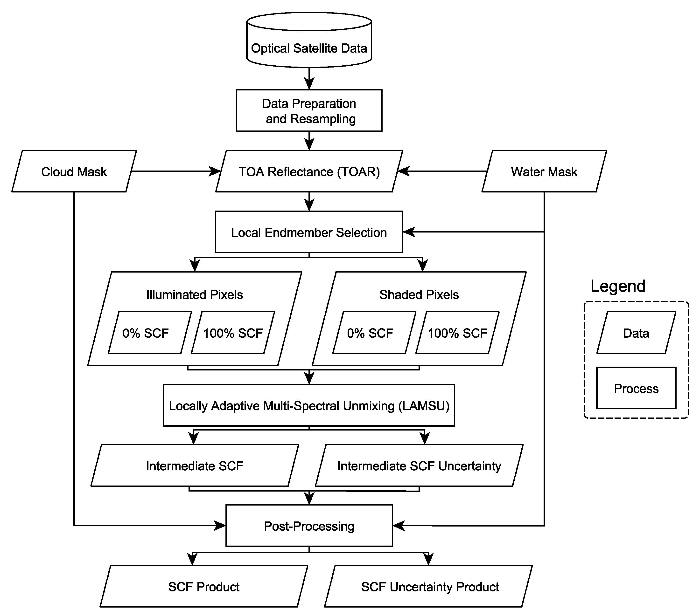
2.2. Methodology
2.2.1. Pre-Processing
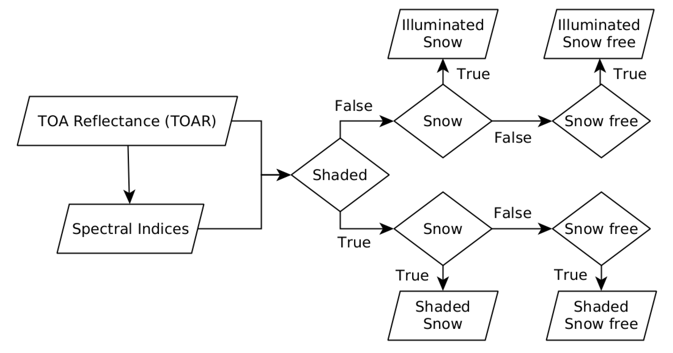
2.2.2. Local Endmember Selection
2.2.3. Locally Adaptive MultiSpectral Unmixing
2.2.4. Post-Processing
2.3. Validation of LAMSU SCF Estimates
3. Results
3.1. Validation with WorldView-2/3 Imagery
3.2. High-Resolution Sensor Application
3.3. Medium-Resolution Sensor Application and Intercomparison
4. Discussion
5. Conclusions
Author Contributions
Funding
Data Availability Statement
Acknowledgments
Conflicts of Interest
Appendix A. Dataset Details
Appendix A.1. LAMSU Input, Validation and Intercomparison Datasets

| № | Scene ID | Date |
|---|---|---|
| 1 | S2A_MSIL1C_20200401T102021_N0209_R065_T32TPS_20200401T123732 | 1 April 2020 |
| 2 | S2A_MSIL1C_20200401T102021_N0209_R065_T32TPT_20200401T123732 | 1 April 2020 |
| 3 | S2B_MSIL1C_20200403T100549_N0209_R022_T32TNR_20200403T130157 | 3 April 2020 |
| 4 | S2B_MSIL1C_20200403T100549_N0209_R022_T32TNS_20200403T130157 | 3 April 2020 |
| 5 | S2B_MSIL1C_20200403T100549_N0209_R022_T32TPR_20200403T130157 | 3 April 2020 |
| 6 | S2B_MSIL1C_20200403T100549_N0209_R022_T32TPS_20200403T130157 | 3 April 2020 |
| 7 | S2B_MSIL1C_20200403T100549_N0209_R022_T32TPT_20200403T130157 | 3 April 2020 |
| 8 | LC08_L1TP_190027_20200402_20200822_02_T1 | 2 April 2020 |
| 9 | LC08_L1TP_190028_20200402_20200822_02_T1 | 2 April 2020 |
| 10 | S3B_OL_1_EFR_20200402T094445_20200402T094745_20200403T130637_0180_037_193_2160_LN1_O_NT_002 | 2 April 2020 |
| S3B_SL_1_RBT_20200402T094445_20200402T094745_20200403T145347_0180_037_193_2160_LN2_O_NT_004 | ||
| 11 | SVI01_npp_d20200402_t1138030_e1143434_b43685_ c20200402154344482690_nobc_ops | 2 April 2020 |
| SVI02_npp_d20200402_t1138030_e1143434_b43685_ c20200402154344489621_nobc_ops | ||
| SVM04_npp_d20200402_t1138030_e1143434_b43685_ c20200402154344475375_nobc_ops | ||
| SVM10_npp_d20200402_t1138030_e1143434_b43685_ c20200402154344428499_nobc_ops | ||
| SVM11_npp_d20200402_t1138030_e1143434_b43685_ c20200402154344434443_nobc_ops | ||
| 13 | MOD021KM.A2020093.1050.061.2020093191243 | 2 April 2020 |
| Ref. № | WorldView Scene ID | |||||
|---|---|---|---|---|---|---|
| Date | Bands | Resolution | Location | Center Longitude, Latitude | Solar Elevation Angle | |
| Comparison № Landsat 8/Sentinel 2 Scene ID Snow-Free Snow | ||||||
| 1 | WV2_OPER_WV1_4B__2A_20150626T130722_N65-304_W018-337_0001_v0100 | |||||
| 26-06-2015 | 4 | 2 m × 2 m | Eyjafjarðarsveit, Iceland | −18.3362, 65.3035 | 48.2 | |
| 1 LC08_L1TP_220014_20150626_20200909_02_T 174.8% 25.2% | ||||||
| 2 | WV2_OPER_WV1_4B__2A_20200827T101318_N45-537_E007-279_0001_v0100 | |||||
| 27-08-2020 | 3 | 0.5 m × 0.5 m | Aosta Valley, Italy | 7.2800, 45.5375 | 50.6 | |
|
1 LC08_L1TP_195028_20200827_20200905_02_T 149.0% 51.0% 2 S2B_MSIL1C_20200827T102559_N0209_R108_T32TLR 32.6% 67.4% | ||||||
| 3 | WV2_OPER_WV1_4B__2A_20210806T103439_N45-541_E007-314_0001_v0100 | |||||
| 06-08-2021 | 3 | 0.4 m × 0.4 m | Aosta Valley, Italy | 7.3138, 45.5414 | 58.4 | |
| 1 S2B_MSIL1C_20210809T101559_N0301_R065_T32TLR 75.5% 24.5% | ||||||
| 4 | WV3_OPER_WV1_4B__2A_20200623T104458_N45-538_E007-317_0001_v0100 | |||||
| 23-06-2020 | 3 | 0.3 m × 0.3 m | Aosta Valley, Italy | 7.3171, 45.5388 | 66.0 | |
|
1 LC08_L1TP_195028_20200624_20200824_02_T1 12.6% 87.4% 2 S2A_MSIL1C_20200623T103031_N0209_R108_T32TLR 12.4% 87.6% | ||||||
| 5 | WV3_OPER_WV1_8B__2A_20201122T104312_N45-409_E007-036_0001_v0100 | |||||
| 22-11-2020 | 8 | 1.2 m × 1.2 m | Val-d’Isère, France | 7.0381, 45.4096 | 24.0 | |
| 1 S2B_MSIL1C_20201125T103349_N0209_R108_T32TLR 39.0% 61.0% | ||||||
Appendix A.2. Worldview-2/3 Classification


Appendix B. LAMSU SCF Examples


References
- Estilow, T.W.; Young, A.H.; Robinson, D.A. A long-term Northern Hemisphere snow cover extent data record for climate studies and monitoring. Earth Syst. Sci. Data 2015, 7, 137–142. [Google Scholar] [CrossRef]
- Barnett, T.; Adam, J.; Lettenmaier, D. Potential Impacts of a Warming Climate on Water Availability in Snow-Dominated Regions. Nature 2005, 438, 303–309. [Google Scholar] [CrossRef]
- Vikhamar, D.; Solberg, R. Snow-cover mapping in forests by constrained linear spectral unmixing of MODIS data. Remote Sens. Environ. 2003, 88, 309–323. [Google Scholar] [CrossRef]
- Dankers, R.; Feyen, L. Flood hazard in Europe in an ensemble of regional climate scenarios. J. Geophys. Res. Atmos. 2009, 114. [Google Scholar] [CrossRef]
- Krøgli, I.K.; Devoli, G.; Colleuille, H.; Boje, S.; Sund, M.; Engen, I.K. The Norwegian forecasting and warning service for rainfall- and snowmelt-induced landslides. Nat. Hazards Earth Syst. Sci. 2018, 18, 1427–1450. [Google Scholar] [CrossRef]
- Robinson, D.A.; Estilow, T.W. Rutgers Northern Hemisphere 24 km Weekly Snow Cover Extent, September 1980 Onward, Version 1. 2021. Available online: https://nsidc.org/data/g10035/versions/1 (accessed on 12 July 2022).
- U.S. National Ice Center. IMS Daily Northern Hemisphere Snow and Ice Analysis at 1 km, 4 km, and 24 km Resolutions, Version 1. 2008. Available online: https://nsidc.org/data/g02156/versions/1 (accessed on 11 July 2022).
- Hori, M.; Sugiura, K.; Kobayashi, K.; Aoki, T.; Tanikawa, T.; Kuchiki, K.; Niwano, M.; Enomoto, H. A 38-year (1978–2015) Northern Hemisphere daily snow cover extent product derived using consistent objective criteria from satellite-borne optical sensors. Remote Sens. Environ. 2017, 191, 402–418. [Google Scholar] [CrossRef]
- Nagler, T.; Schwaizer, G.; Mölg, N.; Keuris, L.; Hetzenecker, M.; Metsämäki, S. ESA Snow Climate Change Initiative (Snow_cci): Daily global Snow Cover Fraction - viewable snow (SCFV) from MODIS (2000–2020). 2022. Available online: https://catalogue.ceda.ac.uk/uuid/ebe625b6f77945a68bda0ab7c78dd76b (accessed on 1 July 2022).
- Romanov, P. Global Multisensor Automated satellite-based Snow and Ice Mapping System (GMASI) for cryosphere monitoring. Remote Sens. Environ. 2017, 196, 42–55. [Google Scholar] [CrossRef]
- Riggs, G.A.; Hall, D.K.; Tschudi, M.; NASA VIIRS Land SIPS. VIIRS/NPP Snow Cover Daily L3 Global 375m SIN Grid, Version 1. 2019. Available online: https://nsidc.org/data/vnp10a1/versions/1 (accessed on 30 June 2022).
- Hall, D.K.; Riggs, G.A. MODIS/Terra Snow Cover Daily L3 Global 500m SIN Grid. 2016. Available online: https://nsidc.org/data/mod10a1/versions/6 (accessed on 27 June 2022).
- Solberg, R.; Trier, ø.; Breivik, L.A.; Godøy, ø.; Killie, M.; Andreassen, L.M.; Hausberg, J.; Olsen, O. CryoClim—A New System for Cryospheric Climate Monitoring. In Proceedings of the 33rd International Symposium on Remote Sensing of Environment, ISRSE 2009, Stresa, Italy, 4–8 May 2009. [Google Scholar]
- Siljamo, N.; Hyvärinen, O.; Riihelä, A.; Suomalainen, M. MetOp/AVHRR Snow Detection Method for Meteorological Applications. J. Appl. Meteorol. Climatol. 2020, 59, 2001–2019. [Google Scholar] [CrossRef]
- Dozier, J. Spectral signature of alpine snow cover from the landsat thematic mapper. Remote Sens. Environ. 1989, 28, 9–22. [Google Scholar] [CrossRef]
- Salomonson, V.; Appel, I. Estimating fractional snow cover from MODIS using the normalized difference snow index. Remote Sens. Environ. 2004, 89, 351–360. [Google Scholar] [CrossRef]
- Salomonson, V.; Appel, I. Development of the Aqua MODIS NDSI fractional snow cover algorithm and validation results. IEEE Trans. Geosci. Remote Sens. 2006, 44, 1747–1756. [Google Scholar] [CrossRef]
- Gascoin, S.; Barrou Dumont, Z.; Deschamps-Berger, C.; Marti, F.; Salgues, G.; López-Moreno, J.I.; Revuelto, J.; Michon, T.; Schattan, P.; Hagolle, O. Estimating Fractional Snow Cover in Open Terrain from Sentinel-2 Using the Normalized Difference Snow Index. Remote Sens. 2020, 12, 2904. [Google Scholar] [CrossRef]
- Riggs, G.; Hall, D.; Román, M.O. MODIS Snow Products Collection 6.1 User Guide. 2019. Available online: https://nsidc.org/sites/default/files/c61_modis_snow_user_guide.pdf (accessed on 24 August 2022).
- Riggs, G.; Hall, D.; Vuyovich, C.; DiGirolamo, N. Development of Snow Cover Frequency Maps from MODIS Snow Cover Products. Remote Sens. 2022, 14, 5661. [Google Scholar] [CrossRef]
- Jing, Y.; Li, X.; Shen, H. STAR NDSI collection: A cloud-free MODIS NDSI dataset (2001–2020) for China. Earth Syst. Sci. Data 2022, 14, 3137–3156. [Google Scholar] [CrossRef]
- HR-S&I Consortium. Algorithm Theoretical Basis Document for Snow Products Based on Sentinel-2 (COSIMS-DT-062-MAG_ATBD_SNOW). 2022. Available online: https://land.copernicus.eu/user-corner/technical-library/hrsi-snow-atbd (accessed on 28 June 2022).
- Painter, T.H.; Dozier, J.; Roberts, D.A.; Davis, R.E.; Green, R.O. Retrieval of subpixel snow-covered area and grain size from imaging spectrometer data. Remote Sens. Environ. 2003, 85, 64–77. [Google Scholar] [CrossRef]
- Painter, T.H.; Rittger, K.; McKenzie, C.; Slaughter, P.; Davis, R.E.; Dozier, J. Retrieval of subpixel snow covered area, grain size, and albedo from MODIS. Remote Sens. Environ. 2009, 113, 868–879. [Google Scholar] [CrossRef]
- Bair, E.H.; Stillinger, T.; Dozier, J. Snow Property Inversion From Remote Sensing (SPIReS): A Generalized Multispectral Unmixing Approach With Examples From MODIS and Landsat 8 OLI. IEEE Trans. Geosci. Remote Sens. 2021, 59, 7270–7284. [Google Scholar] [CrossRef]
- Dietz, A.J.; Kuenzer, C.; Gessner, U.; Dech, S. Remote sensing of snow—A review of available methods. Int. J. Remote Sens. 2012, 33, 4094–4134. [Google Scholar] [CrossRef]
- Rittger, K.; Painter, T.H.; Dozier, J. Assessment of methods for mapping snow cover from MODIS. Adv. Water Resour. 2013, 51, 367–380. [Google Scholar] [CrossRef]
- Masson, T.; Dumont, M.; Mura, M.D.; Sirguey, P.; Gascoin, S.; Dedieu, J.P.; Chanussot, J. An Assessment of Existing Methodologies to Retrieve Snow Cover Fraction from MODIS Data. Remote Sens. 2018, 10, 619. [Google Scholar] [CrossRef]
- Aalstad, K.; Westermann, S.; Bertino, L. Evaluating satellite retrieved fractional snow-covered area at a high-Arctic site using terrestrial photography. Remote Sens. Environ. 2020, 239, 111618. [Google Scholar] [CrossRef]
- Stillinger, T.; Rittger, K.; Raleigh, M.S.; Michell, A.; Davis, R.E.; Bair, E.H. Landsat, MODIS, and VIIRS snow cover mapping algorithm performance as validated by airborne lidar datasets. Cryosphere Discuss. 2022, 2022. [Google Scholar] [CrossRef]
- Dobreva, I.D.; Klein, A.G. Fractional snow cover mapping through artificial neural network analysis of MODIS surface reflectance. Remote Sens. Environ. 2011, 115, 3355–3366. [Google Scholar] [CrossRef]
- Czyzowska-Wisniewski, E.H.; van Leeuwen, W.J.; Hirschboeck, K.; Marsh, S.E.; Wisniewski, W.T. Fractional snow cover estimation in complex alpine-forested environments using an artificial neural network. Remote Sens. Environ. 2015, 156, 403–417. [Google Scholar] [CrossRef]
- Hofmeister, F.; Arias-Rodriguez, L.; Premier, V.; Marin, C.; Notarnicola, C.; Disse, M.; Chiogna, G. Intercomparison of Sentinel-2 and modelled snow cover maps in a high-elevation Alpine catchment. J. Hydrol. X 2022, 15, 100123. [Google Scholar] [CrossRef]
- Barella, R.; Marin, C.; Gianinetto, M.; Notarnicola, C. A Novel Approach to High Resolution Snow Cover Fraction Retrieval in Mountainous Regions. In Proceedings of the IGARSS 2022 - 2022 IEEE International Geoscience and Remote Sensing Symposium, Kuala Lumpur, Malaysia, 17–22 July 2022; pp. 3856–3859. [Google Scholar] [CrossRef]
- Chen, Y.; Hall, A.; Liou, K.N. Application of three-dimensional solar radiative transfer to mountains. J. Geophys. Res. Atmos. 2006, 111. [Google Scholar] [CrossRef]
- Sirguey, P.; Mathieu, R.; Arnaud, Y. Subpixel monitoring of the seasonal snow cover with MODIS at 250 m spatial resolution in the Southern Alps of New Zealand: Methodology and accuracy assessment. Remote Sens. Environ. 2009, 113, 160–181. [Google Scholar] [CrossRef]
- Kuter, S.; Bolat, K.; Akyurek, Z. A machine learning-based accuracy enhancement on EUMETSAT H-SAF H35 effective snow-covered area product. Remote Sens. Environ. 2022, 272, 112947. [Google Scholar] [CrossRef]
- Nolin, A.W.; Dozier, J.; Mertes, L.A.K. Mapping alpine snow using a spectral mixture modeling technique. Ann. Glaciol. 1993, 17, 121–124. [Google Scholar] [CrossRef]
- Cannistra, A.F.; Shean, D.E.; Cristea, N.C. High-resolution CubeSat imagery and machine learning for detailed snow-covered area. Remote Sens. Environ. 2021, 258, 112399. [Google Scholar] [CrossRef]
- Defourny, P.; Lamarche, C.; Bontemps, S.; De Maet, T.; Van Bogaert, E.; Moreau, I.; Brockmann, C.; Boettcher, M.; Kirches, G.; Wevers, J.; et al. Land Cover CCI Product User Guide Version 2. Technical Report. 2017. Available online: https://maps.elie.ucl.ac.be/CCI/viewer/download/ESACCI-LC-Ph2-PUGv2_2.0.pdf (accessed on 18 April 2022).
- Pekel, J.F.; Cottam, A.; Gorelick, N.; Belward, A.S. High-resolution mapping of global surface water and its long-term changes. Nature 2016, 540, 418–422. [Google Scholar] [CrossRef] [PubMed]
- Porter, C.; Morin, P.; Howat, I.; Noh, M.J.; Bates, B.; Peterman, K.; Keesey, S.; Schlenk, M.; Gardiner, J.; Tomko, K.; et al. ArcticDEM. 2018. Available online: https://dataverse.harvard.edu/dataset.xhtml?persistentId=doi:10.7910/DVN/OHHUKH (accessed on 18 April 2022).
- González, J.C.G.; Redondo, J.A.; Garzón, A. EU-DEM Upgrade: Documentation EEA User Manual (C4EO17 1/2). 2015. Available online: https://land.copernicus.eu/user-corner/technical-library/eu-dem-v1-1-user-guide (accessed on 9 May 2022).
- Nagler, T.; Ripper, E.; Rott, H. Preparations for Snow Monitoring using Sentinel-3 SLSTR and OLCI. 2012. Available online: https://www.researchgate.net/publication/258776433_Preparation_for_Snow_Cover_Monitoring_Using_Sentinel-1_and_Sentinel-3_Data (accessed on 3 May 2022).
- Rouse, J.W.; Haas, R.H.; Schell, J.A.; Deering, D.W. Monitoring Vegetation Systems in the Great Plains with ERTS. 1973. Available online: https://ntrs.nasa.gov/citations/19740022614 (accessed on 30 August 2022).
- Jiang, Z.; Huete, A.R.; Didan, K.; Miura, T. Development of a two-band enhanced vegetation index without a blue band. Remote Sens. Environ. 2008, 112, 3833–3845. [Google Scholar] [CrossRef]
- Chang, C.I. Spectral information divergence for hyperspectral image analysis. In Proceedings of the IEEE 1999 International Geoscience and Remote Sensing Symposium. IGARSS’99, Hamburg, Germany, 8 June–2 July 1999; Volume 1, pp. 509–511. [Google Scholar] [CrossRef]
- Fortune, S. A sweepline algorithm for Voronoi diagrams. Algorithmica 1987, 2. [Google Scholar] [CrossRef]
- Stark, P.; Parker, R. Bounded-variable least-squares: An algorithm and applications. Comput. Stat. 1995, 129–141. [Google Scholar]
- Chen, T.; Guestrin, C. XGBoost. In Proceedings of the Proceedings of the 22nd ACM SIGKDD International Conference on Knowledge Discovery and Data Mining, San Francisco, CA, USA, 13–17 August 2016. [Google Scholar] [CrossRef]
- Hastie, T.; Tibshirani, R.; Friedman, J.H. Boosting and Additive Trees. In The Elements of Statistical Learning, 2nd ed.; Springer: Berlin/Heidelberg, Germany, 2009; pp. 337–384. [Google Scholar]
- Kernighan, B.W.; Ritchie, D.M. The C Programming Language; Prentice Hall: Englewood Cliffs, NJ, USA, 2006. [Google Scholar]
- OpenMP Architecture Review Board. OpenMP Application Program Interface Version 4.5. 2015. Available online: https://www.openmp.org/wp-content/uploads/openmp-4.5.pdf (accessed on 20 January 2022).


| Satellite | Sensor | Bands |
|---|---|---|
| Sentinel-2 A/B | MSI | 2, 3, 4, 8 (10 m) 5, 6, 7, 8A, 11, 12 (20 m) 1, 9, 10 (60 m) |
| Landsat 8/9 | OLI(-2) | 8 (15 m) 1, 2, 3, 4, 5, 6, 7, 9 (30 m) |
| Sentinel-3 A/B | OLCI | Oa01, Oa02, Oa03, Oa04, Oa05, Oa06, Oa07, Oa08, Oa09, Oa10, Oa11, Oa12, Oa13, Oa14, Oa15, Oa16, Oa17, Oa18, Oa19, Oa20, Oa21 (300 m) |
| Sentinel-3 A/B | SLSTR | S1, S2, S3, S4, S5, S6 (500 m) |
| Suomi NPP | VIIRS | i01, i02 (375 m) m04, m10, m11 (750 m) |
| Terra | MODIS | 1, 2 (250 m) 3, 4, 5, 6, 7 (500 m) (all bands are also available as aggregated 1 km products) |
| WorldView-2 | WV110 | panchromatic (1) (0.41 m) multispectral (8) (1.64 m) |
| WorldView-3 | WV110 | panchromatic (1) (0.31 m) multispectral (8) (1.24 m) |
| № | Spectral Index | Characteristic |
|---|---|---|
| 1 | Increases with snow presence and shade. This index is also known as the NDSI [15]. | |
| 2 | Increases with vegetation presence and decreases within shade. This index is also known as the NDVI [45]. | |
| 3 | Increases with vegetation presence and decreases within shade. This index is also known as the two-band EVI [46]. | |
| 4 | Increases with snow presence but is more robust and sensitive to snow in the shade than NDSI. | |
| 5 | Same as (4) but is less sensitive to vegetation. | |
| 6 | Same as (4) but is more sensitive to shade than snow. | |
| 7 | Same as (4) but is less sensitive to snow. | |
| 8 | Increases with shade and is close to zero for snow. | |
| 9 | Increases with snow presence and shade. Slightly lower sensitivity to snow presence and shade than (1). | |
| 10 | Increases with snow presence and shade. Lower sensitivity to snow presence and shade (in particular in illuminated areas) than (1). | |
| 11 | Increases with snow presence and shade. Lower sensitivity to snow presence and shade (in particular in illuminated areas) than (1). |
| LAMSU | FRA6T [17] | |||||
|---|---|---|---|---|---|---|
| Reference № | L8/S2 | Bias (%) | RMSE (%) | Bias (%) | RMSE (%) | N (#) |
| 1 | L8 | −3.30 | 10.80 | 4.12 | 13.54 | 29652 |
| 2 | L8 | 8.10 | 21.45 | 17.37 | 35.20 | 18203 |
| S2 | 3.85 | 18.56 | 7.92 | 25.09 | 12327 | |
| 3 | S2 | 0.62 | 16.79 | 8.36 | 26.21 | 102602 |
| 4 | L8 | 0.42 | 9.30 | 3.37 | 13.18 | 13115 |
| S2 | 0.87 | 10.10 | 4.33 | 14.38 | 45732 | |
| 5 | S2 | −1.95 | 14.17 | 9.87 | 27.59 | 84644 |
| Overall | 0.15 | 14.28 | 7.21 | 23.48 | 306275 | |
| RMSE | Sentinel-2 MSI | Landsat 8 OLI | Sentinel-3 SLSTR/OLCI | Suomi NPP VIIRS | Terra MODIS | |
|---|---|---|---|---|---|---|
| Bias | ||||||
| Sentinel-2 MSI | - | - | 9.68 | 7.35 | 6.99 | |
| Landsat 8 OLI | - | - | 4.92 | 4.33 | 5.32 | |
| Sentinel-3 SLSTR/OLCI | −1.46 | 0.76 | - | 8.19 | 8.93 | |
| Suomi NPP VIIRS | −0.34 | 1.28 | 0.65 | - | 8.86 | |
| Terra MODIS | 0.47 | 1.71 | 2.16 | 2.15 | - | |
| № | Date | Tile | Bias | RMSE | Bias | RMSE | Bias | RMSE |
|---|---|---|---|---|---|---|---|---|
| Sentinel-2 MSI | Sentinel-3 SLSTR/OLCI | Suomi NPP VIIRS | Terra MODIS | |||||
| 1 | 1 April 2020 | 32TPS | 0.59 | 7.15 | 0.68 | 6.72 | 1.19 | 7.59 |
| 2 | 1 April 2020 | 32TPT | 2.21 | 8.63 | 1.97 | 7.73 | 3.36 | 8.35 |
| 3 | 3 April 2020 | 32TNR | −6.00 | 14.83 | −1.97 | 7.82 | −1.61 | 6.23 |
| 4 | 3 April 2020 | 32TNS | −1.93 | 10.06 | −1.34 | 7.95 | −0.29 | 8.37 |
| 5 | 3 April 2020 | 32TPR | −3.07 | 10.60 | 0.08 | 6.83 | 0.42 | 5.68 |
| 6 | 3 April 2020 | 32TPS | −1.53 | 8.62 | −0.86 | 6.98 | −0.10 | 7.67 |
| 7 | 3 April 2020 | 32TPT | −0.47 | 7.88 | −1.16 | 6.57 | 0.30 | 5.07 |
| Landsat 8 OLI | Sentinel-3 SLSTR/OLCI | Suomi NPP VIIRS | Terra MODIS | |||||
| 1 | 2 April 2020 | 190027 | 0.42 | 5.24 | 0.98 | 4.60 | 1.68 | 5.81 |
| 2 | 2 April 2020 | 190028 | 1.09 | 4.60 | 1.58 | 4.06 | 1.73 | 4.82 |
Disclaimer/Publisher’s Note: The statements, opinions and data contained in all publications are solely those of the individual author(s) and contributor(s) and not of MDPI and/or the editor(s). MDPI and/or the editor(s) disclaim responsibility for any injury to people or property resulting from any ideas, methods, instructions or products referred to in the content. |
© 2023 by the authors. Licensee MDPI, Basel, Switzerland. This article is an open access article distributed under the terms and conditions of the Creative Commons Attribution (CC BY) license (https://creativecommons.org/licenses/by/4.0/).
Share and Cite
Keuris, L.; Hetzenecker, M.; Nagler, T.; Mölg, N.; Schwaizer, G. An Adaptive Method for the Estimation of Snow-Covered Fraction with Error Propagation for Applications from Local to Global Scales. Remote Sens. 2023, 15, 1231. https://doi.org/10.3390/rs15051231
Keuris L, Hetzenecker M, Nagler T, Mölg N, Schwaizer G. An Adaptive Method for the Estimation of Snow-Covered Fraction with Error Propagation for Applications from Local to Global Scales. Remote Sensing. 2023; 15(5):1231. https://doi.org/10.3390/rs15051231
Chicago/Turabian StyleKeuris, Lars, Markus Hetzenecker, Thomas Nagler, Nico Mölg, and Gabriele Schwaizer. 2023. "An Adaptive Method for the Estimation of Snow-Covered Fraction with Error Propagation for Applications from Local to Global Scales" Remote Sensing 15, no. 5: 1231. https://doi.org/10.3390/rs15051231
APA StyleKeuris, L., Hetzenecker, M., Nagler, T., Mölg, N., & Schwaizer, G. (2023). An Adaptive Method for the Estimation of Snow-Covered Fraction with Error Propagation for Applications from Local to Global Scales. Remote Sensing, 15(5), 1231. https://doi.org/10.3390/rs15051231